Eratosthenes sieve and the gaps between primes

Fred B. Holt and Helgi Rudd Address: fbholt@uw.edu ; 4311-11th Ave NE #500, Seattle, WA 98105; 48B York Place, Prahran, Australia 3181

Date: 25 Aug 2014

Abstract.

A few years ago we identified a recursion that works directly with the gaps among the generators in each stage of Eratosthenes sieve. This recursion provides explicit enumerations of sequences of gaps among the generators, which sequences are known as constellations.

By studying this recursion on the cycles of gaps across stages of Eratosthenes sieve, we are able to provide evidence on a number of open problems regarding gaps between prime numbers. The basic counts of short constellations in the cycles of gaps provide evidence toward the twin prime conjecture and toward resolving a series of questions posed by Erdös and Turán. The dynamic system underlying the recursion provides evidence toward Polignac’s conjecture and in support of the estimates made for gaps among primes by Hardy and Littlewood in Conjecture B of their 1923 paper.

Key words and phrases:

primes, twin primes, gaps, prime constellations, Eratosthenes sieve, primorial numbers, Polignac’s conjecture

1991 Mathematics Subject Classification

11N05, 11A41, 11A07

1. Introduction

We work with the prime numbers in ascending order, denoting the ${k}^{\rm th}$ prime by $p_{k}$ . Accompanying the sequence of primes is the sequence of gaps between consecutive primes. We denote the gap between $p_{k}$ and $p_{k+1}$ by $g_{k}=p_{k+1}-p_{k}.$ These sequences begin

\begin{array}[]{rrrrrrc}p_{1}=2,&p_{2}=3,&p_{3}=5,&p_{4}=7,&p_{5}=11,&p_{6}=13,&\ldots\\ g_{1}=1,&g_{2}=2,&g_{3}=2,&g_{4}=4,&g_{5}=2,&g_{6}=4,&\ldots\end{array}

A number $d$ is the difference between prime numbers if there are two prime numbers, $p$ and $q$ , such that $q-p=d$ . There are already many interesting results and open questions about differences between prime numbers; a seminal and inspirational work about differences between primes is Hardy and Littlewood’s 1923 paper [11].

A number $g$ is a gap between prime numbers if it is the difference between consecutive primes; that is, $p=p_{i}$ and $q=p_{i+1}$ and $q-p=g$ . Differences of length $2$ or $4$ are also gaps; so open questions like the Twin Prime Conjecture, that there are an infinite number of gaps $g_{k}=2$ , can be formulated as questions about differences as well.

A constellation among primes [18] is a sequence of consecutive gaps between prime numbers. Let $s=a_{1}a_{2}\cdots a_{k}$ be a sequence of $k$ numbers. Then $s$ is a constellation among primes if there exists a sequence of $k+1$ consecutive prime numbers $p_{i}p_{i+1}\cdots p_{i+k}$ such that for each $j=1,\ldots,k$ , we have the gap $p_{i+j}-p_{i+j-1}=a_{j}$ . Equivalently, $s$ is a constellation if for some $i$ and all $j=1,\ldots,k$ , $a_{j}=g_{i+j}$ .

We do not study the gaps between primes directly. Instead, we study the cycle of gaps ${\mathcal{G}}({p}^{\#})$ at each stage of Eratosthenes sieve. Here, ${p}^{\#}$ is the primorial of $p$ , which is the product of all primes from $2$ up to and including $p$ . ${\mathcal{G}}({p}^{\#})$ is the cycle of gaps among the generators of ${\mathbb{Z}}\bmod{p}^{\#}$ . These generators and their images through the counting numbers are the candidate primes after Eratosthenes sieve has run through the stages from $2$ to $p$ . All of the remaining primes are among these candidates.

There is a substantial amount of structure preserved in the cycle of gaps from one stage of Eratosthenes sieve to the next, from ${\mathcal{G}}({p_{k}}^{\#})$ to ${\mathcal{G}}({p_{k+1}}^{\#})$ . This structure is sufficient to enable us to give exact counts for gaps and for sufficiently short constellations in ${\mathcal{G}}({p}^{\#})$ across all stages of the sieve.

1.1. Some conjectures and open problems regarding gaps between primes.

Open problems regarding gaps and constellations between prime numbers include the following.

•

Twin Prime Conjecture - There are infinitely many pairs of consecutive primes with gap $g=2$ .
•

Polignac’s Conjecture - For every even number $2n$ , there are infinitely many pairs of consecutive primes with gap $g=2n$ .
•

Primorial conjecture - The gap $g=6={3}^{\#}$ occurs more often than the gap $g=2$ , and eventually the gap $g=30={5}^{\#}$ occurs more often than the gap $g=6$ .
•

HL Conjecture B - From page 42 of Hardy and Littlewood [11]: for any even $k$ , the number of prime pairs $q$ and $q+k$ such that $q+k<n$ is approximately

$2C_{2}\frac{n}{(\log n)^{2}}\prod_{p\neq 2,\;p|k}\frac{p-1}{p-2}.$
•

ET Spikes - From p.377 of Erdös and Turán [6], that it is very probable that

$\lim\sup\frac{g_{k+1}}{g_{k}}=\infty\makebox[5.42003pt]{}{\rm and}\makebox[5.42003pt]{}\lim\inf\frac{g_{k+1}}{g_{k}}=0.$
•

ET Superlinearity - On p.378 of Erdös and Turán [6], the open question is posed whether for every $k>1$ there are infinitely many $n$ such that

$g_{n}<g_{n+1}<g_{n+2}<\cdots<g_{n+k}.$

These problems and others regarding the gaps and differences among primes are usually approached through sophisticated probabilistic models, rooted in the prime number theorem. Seminal works for our studies include [11, 12, 4]. Several estimates on gaps derived from these models have been corroborated computationally. These computations have addressed the occurrence of twin primes [2, 15, 17, 13, 14], and some have corroborated the estimates in Conjecture B for other gaps [1, 10].

Work on specific constellations among primes includes the study of prime quadruplets [11, 3], which corresponds to the constellation $2,4,2$ . This is two pairs of twin primes separated by a gap of $4$ , the densest possible occurrence of primes in the large. The estimates for prime quadruplets have also been supported computationally [16].

1.2. Analogues demonstrated for Eratosthenes sieve.

We do not resolve any of the open problems as stated above for gaps between primes. However, we are able to resolve their analogues for gaps in the stages of Eratosthenes sieve. Through our work below we prove the following.

•

Twin Generators - The number of gaps $g=2$ in the cycle of gaps ${\mathcal{G}}({p_{k}}^{\#})$ is

$N_{2}({p_{k}}^{\#})=\prod_{q=3}^{p_{k}}(q-2).$
•

Polignac’s Conjecture and HL Conjecture B - For every even number $2n$ , the gap $g=2n$ arises at some stage in the cycle of gaps ${\mathcal{G}}({p}^{\#})$ and thereafter the ratio of its occurrences in a cycle of gaps to the number of gaps $g=2$ approaches the asymptotic value suggested by Hardy and Littlewood’s Conjecture B

$\lim_{p\longrightarrow\infty}\frac{N_{2n}({p}^{\#})}{N_{2}({p}^{\#})}=\prod_{q>2,\;q|n}\frac{q-1}{q-2}.$
•

Primorial conjecture - The dynamic system that yields the preceding result tells us that for primorial gaps $g={p_{k-1}}^{\#}$ and $g={p_{k}}^{\#}$ ,

$\lim_{q\longrightarrow\infty}\frac{N_{{p_{k}}^{\#}}({q}^{\#})}{N_{{p_{k-1}}^{\#}}({q}^{\#})}=\frac{p_{k}-1}{p_{k}-2}.$

The eigenvalues of the dynamic system indicate how quickly the values will converge to the asymptotic ratio.
•

ET Spikes - For gaps in the cycles of gaps,

$\lim\sup\frac{g_{k+1}}{g_{k}}=\infty\makebox[5.42003pt]{}{\rm and}\makebox[5.42003pt]{}\lim\inf\frac{g_{k+1}}{g_{k}}=0.$

In particular, for $g_{k}=2$ , the adjacent gaps $g_{k-1}$ and $g_{k+1}$ become arbitrarily large in later stages of the sieve.
•

ET Superlinear growth - For every $k>1$ there is a cycle of gaps ${\mathcal{G}}({p}^{\#})$ with a constellation of $k$ consecutive gaps such that

$g_{n+1}<g_{n+2}<\cdots<g_{n+k}.$

This constellation persists across all subsequent stages of the sieve, and its population increases by the factor $p-k-1$ at each stage.
•

ET Superlinear decay - For every $k>1$ there is a cycle of gaps ${\mathcal{G}}({p}^{\#})$ with a constellation of $k$ consecutive gaps such that

$g_{n+1}>g_{n+2}>\cdots>g_{n+k}.$

This constellation persists across all subsequent stages of the sieve, and its population increases by the factor $p-k-1$ at each stage.

These results are deterministic, not probabilistic. We develop a population model below that describes the growth of the populations of various gaps in the cycle of gaps, across the stages of Eratosthenes sieve.

All gaps between prime numbers arise in a cycle of gaps. To connect our results to the desired results on gaps between primes, we need to better understand how gaps survive later stages of the sieve, to be affirmed as gaps between primes.

2. The cycle of gaps

After the first two stages of Eratosthenes sieve, we have removed the multiples of $2$ and $3$ . The candidate primes at this stage of the sieve are

(1),5,7,11,13,17,19,23,25,29,31,35,37,41,43,\ldots

We investigate the structure of these sequences of candidate primes by studying the cycle of gaps in the fundamental cycle.

For example, for the candidate primes listed above, the first gap from $1$ to $5$ is $g=4$ , the second gap from $5$ to $7$ is $g=2$ , then $g=4$ from $7$ to $11$ , and so on. The cycle of gaps ${\mathcal{G}}({3}^{\#})$ is $42$ . To reduce visual clutter, we write the cycles of gaps as a concatenation of single digit gaps, reserving the use of commas to delineate gaps of two or more digits.

{\mathcal{G}}({3}^{\#})=42,\makebox[5.42003pt]{}{\rm with}\makebox[5.42003pt]{}g_{3,1}=4\makebox[5.42003pt]{}{\rm and}\makebox[5.42003pt]{}g_{3,2}=2.

Advancing Eratosthenes sieve one more stage, we identify $5$ as the next prime and remove the multiples of $5$ from the list of candidates, leaving us with

(1),7,11,13,17,19,23,29,31,37,41,43,47,49,53,59,61,\ldots

We calculate the cycle of gaps at this stage to be ${\mathcal{G}}({5}^{\#})=64242462.$

We note that ${\mathcal{G}}({p}^{\#})$ consists of $\phi({p}^{\#})$ gaps that sum to ${p}^{\#}$ .

2.1. Recursion on the cycle of gaps

There is a nice recursion which produces ${\mathcal{G}}(p_{k+1})$ directly from ${\mathcal{G}}(p_{k})$ . We concatenate $p_{k+1}$ copies of ${\mathcal{G}}(p_{k})$ , and add together certain gaps as indicated by the entry-wise product $p_{k+1}*{\mathcal{G}}(p_{k})$ .

Lemma 2.1.

The cycle of gaps ${\mathcal{G}}({p_{k+1}}^{\#})$ is derived recursively from ${\mathcal{G}}({p_{k}}^{\#})$ . Each stage in the recursion consists of the following three steps:

R1.

Determine the next prime, $p_{k+1}=g_{k,1}+1$ .
R2.

Concatenate $p_{k+1}$ copies of ${\mathcal{G}}({p_{k}}^{\#})$ .
R3.

Add adjacent gaps as indicated by the elementwise product $p_{k+1}*{\mathcal{G}}({p_{k}}^{\#})$ : let $i_{1}=1$ and add together $g_{i_{1}}+g_{i_{1}+1}$ ; then for $n=1,\ldots,\phi(N)$ , add $g_{j}+g_{j+1}$ and let $i_{n+1}=j$ if the running sum of the concatenated gaps from $g_{i_{n}}$ to $g_{j}$ is $p_{k+1}*g_{n}.$

Proof.

Let ${\mathcal{G}}({p_{k}}^{\#})$ be the cycle of gaps for the stage of Eratosthenes sieve after the multiples of the primes up through $p_{k}$ have been removed. We show that the recursion R1-R2-R3 on ${\mathcal{G}}({p_{k}}^{\#})$ produces the cycle of gaps for the next stage, corresponding to the removal of multiples of $p_{k+1}$ .

There is a natural one-to-one correspondence between the gaps in the cycle of gaps ${\mathcal{G}}({p_{k}}^{\#})$ and the generators of ${\mathbb{Z}}\bmod{p_{k}}^{\#}$ . For $j=1,\ldots,\phi({p_{k}}^{\#})$ let

(1)

\gamma_{k,j}=1+\sum_{i=1}^{j}g_{i}.

These $\gamma_{k,j}$ are the generators in ${\mathbb{Z}}\bmod{p_{k}}^{\#}$ , with $\gamma_{k,\phi({p_{k}}^{\#})}\equiv 1\bmod{p_{k}}^{\#}$ .

The ${j}^{\rm th}$ candidate prime at this stage of the sieve is given by $\gamma_{k,j}$ .

The next prime $p_{k+1}$ will be $\gamma_{k,1}$ , since this will be the smallest integer both greater than $1$ and coprime to ${p_{k}}^{\#}$ .

The second step of the recursion extends our list of possible primes up to ${p_{k+1}}^{\#}+1$ , the reach of the fundamental cycle for ${p_{k+1}}^{\#}$ . For the gaps $g_{j}$ we extend the indexing on $j$ to cover these concatenated copies. These $p_{k+1}$ concatenated copies of ${\mathcal{G}}({p_{k}}^{\#})$ correspond to all the numbers from $1$ to ${p_{k+1}}^{\#}+1$ which are coprime to ${p_{k}}^{\#}$ . For the set of generators of ${p_{k+1}}^{\#}$ , we need only remove the multiples of $p_{k+1}$ .

The third step removes the multiples of $p_{k+1}$ . Removing a possible prime amounts to adding together the gaps on either side of this entry. The only multiples of $p_{k+1}$ which remain in the copies of ${\mathcal{G}}({p_{k}}^{\#})$ are those multiples all of whose prime factors are greater than $p_{k}$ . After $p_{k+1}$ itself, the next multiple to be removed will be $p_{k+1}^{2}$ .

The multiples we seek to remove are given by $p_{k+1}$ times the generators of ${\mathbb{Z}}\bmod{p_{k}}^{\#}$ . The consecutive differences between these will be given by $p_{k+1}*g_{j}$ , and the sequence $p_{k+1}*{\mathcal{G}}({p_{k}}^{\#})$ suffices to cover the concatenated copies of ${\mathcal{G}}({p_{k}}^{\#})$ . We need not consider any fewer nor any more multiples of $p_{k+1}$ to obtain the generators for ${\mathcal{G}}({p_{k+1}}^{\#})$ .

In the statement of R3, the index $n$ moves through the copy of ${\mathcal{G}}({p_{k}}^{\#})$ being multiplied by $p_{k+1}$ , and the indices $\tilde{i}_{n}$ mark the index $j$ at which the addition of gaps is to occur. The multiples of $p_{k+1}$ in the sieve up through $p_{k}$ are given by $p_{k+1}$ itself and $p_{k+1}*\gamma_{k,j}$ for $j=1,\ldots,\phi({p_{k}}^{\#})$ . The difference between successive multiples is $p_{k+1}*g_{j}$ . ∎

Refer to caption — Figure 1. Illustrating the recursion that produces the gaps for the next stage of Eratosthenes sieve. The cycle of gaps ${\mathcal{G}}({7}^{\#})$ is produced from ${\mathcal{G}}({5}^{\#})$ by concatenating $7$ copies, then adding the gaps indicated by the element-wise product $7*{\mathcal{G}}({5}^{\#})$ .

We call the additions in step R3 the closure of the two adjacent gaps.

The first closure in step R3 corresponds to noting the next prime number $p_{k+1}$ . The remaining closures in step R3 correspond to removing from the candidate primes the composite numbers whose smallest prime factor is $p_{k+1}$ . From step R2, the candidate primes have the form $\gamma+j\cdot{p_{k}}^{\#}$ , for a generator $\gamma$ of ${\mathbb{Z}}\bmod{p_{k}}^{\#}$ .

Example: ${\mathcal{G}}(5)$ . We start with ${\mathcal{G}}(3)=42.$

R1.

$p_{k+1}=5.$
R2.

Concatenate five copies of ${\mathcal{G}}(3)$ :

$4242424242.$
R3.

Add together the gaps after the initial gap $g=4$ and thereafter after cumulative differences of $5*{\mathcal{G}}(3)=20,10$ :
${\mathcal{G}}(5)$ $=$ $4+\overbrace{2424242}^{20}+\overbrace{42\;\;}^{10}$ $=$ $64242462.$
Note that the last addition wraps around the end of the cycle and recloses the gap after the first $4$ .

Example: ${\mathcal{G}}({7}^{\#})$ . As a second example of the recursion, we construct ${\mathcal{G}}({7}^{\#})$ from ${\mathcal{G}}({5}^{\#})=64242462$ . Figure 1 provides an illustration of this construction.

R1.

Identify the next prime, $p_{k+1}=g_{1}+1=7.$
R2.

Concatenate seven copies of ${\mathcal{G}}({5}^{\#})$ :

$\scriptstyle 64242462\;64242462\;64242462\;64242462\;64242462\;64242462\;64242462$

R3.

Add together the gaps after the leading $6$ and thereafter after differences of $7*{\mathcal{G}}({5}^{\#})=42,28,14,28,14,28,42,14$ :

\begin{array}[]{l}{\mathcal{G}}({7}^{\#})\;=\\ {\scriptstyle 6+\overbrace{\scriptstyle 424246264242}^{42}+\overbrace{\scriptstyle 4626424}^{28}+\overbrace{\scriptstyle 2462}^{14}+\overbrace{\scriptstyle 6424246}^{28}+\overbrace{\scriptstyle 2642}^{14}+\overbrace{\scriptstyle 4246264}^{28}+\overbrace{\scriptstyle 242462642424}^{42}+\overbrace{\scriptstyle 62\;}^{14}}\\ =\;{\it 10},2424626424{\it 6}62642{\it 6}46{\it 8}42424{\it 8}64{\it 6}24626{\it 6}4246264242,{\it 10},2\end{array}

The final difference of $14$ wraps around the end of the cycle, from the addition preceding the final $6$ to the addition after the first $6$ .

Remark 2.2.

The following results are easily established for ${\mathcal{G}}(p_{k})$ :

i)

The cycle of gaps ${\mathcal{G}}({p_{k}}^{\#})$ consists of $\phi({p_{k}}^{\#})$ gaps that sum to ${p_{k}}^{\#}$ .
ii)

The first difference between closures is $p_{k+1}*(p_{k+1}-1)$ , which removes $p_{k+1}^{2}$ from the list of candidate primes.
iii)

The last entry in ${\mathcal{G}}({p_{k}}^{\#})$ is always $2$ . This difference goes from $-1$ to $+1$ in ${\mathbb{Z}}\bmod{p_{k}}^{\#}$ .
iv)

The last difference $p_{k+1}*2$ between closures in step R3, wraps from $-p_{k+1}$ to $p_{k+1}$ in ${\mathbb{Z}}\bmod{p_{k+1}}^{\#}$ .
v)

Except for the final $2$ , the cycle of differences is symmetric: $g_{k,j}=g_{k,\phi({p_{k}}^{\#})-j}$ .
vi)

If $m+1$ consecutive gaps have the same value,

$g_{k,j}=g_{k,j+1}=\cdots=g_{k,j+m}=g,$

then $g=0\bmod p$ for all primes $p\leq m+2$ . Note that this constellation corresponds to $m+2$ consecutive primes in arithmetic progression.
vii)

The middle of the cycle ${\mathcal{G}}({p_{k}}^{\#})$ is the sequence

$2^{j},2^{j-1},\ldots,42424,\ldots,2^{j-1},2^{j}$

in which $j$ is the smallest number such that $2^{j+1}>p_{k+1}$ .

There is an interesting fractal character to the recursion. To produce the next cycle of gaps ${\mathcal{G}}({p_{k+1}}^{\#})$ from the current one, ${\mathcal{G}}({p_{k}}^{\#})$ , we concatenate $p_{k+1}$ copies of the current cycle, take an expanded copy of the current cycle, and close gaps as indicated by that expanded copy. In the discrete dynamic system that we develop below, we don’t believe that all of the power in this self-similarity has yet been captured.

2.2. Every possible closure of adjacent gaps occurs exactly once

Theorem 2.3.

Each possible closure of adjacent gaps in the cycle ${\mathcal{G}}({p_{k}}^{\#})$ occurs exactly once in the recursive construction of ${\mathcal{G}}({p_{k+1}}^{\#}).$

Proof.

This is an implication of the Chinese Remainder Theorem. Each entry in ${\mathcal{G}}({p_{k}}^{\#})$ corresponds to one of the generators of ${\mathbb{Z}}\bmod{p_{k}}^{\#}$ . The first gap $g_{1}$ corresponds to $p_{k+1}$ , and thereafter $g_{j}$ corresponds to $\gamma_{k,j}=1+\sum_{i=1}^{j}g_{i}$ . These correspond in turn to unique combinations of nonzero residues modulo the primes $2,3,\ldots,p_{k}$ .

In step R2, we concatenate $p_{k+1}$ copies of ${\mathcal{G}}({p_{k}}^{\#})$ . For each gap $g_{j}$ in ${\mathcal{G}}({p_{k}}^{\#})$ there are $p_{k+1}$ copies of this gap after step R2, corresponding to

\gamma_{k,j}+i\cdot{p_{k}}^{\#}\makebox[10.84006pt]{}{\rm for}\makebox[5.42003pt]{}i=0,\ldots,p_{k+1}-1.

For each copy, the combination of residues for $\gamma_{k,j}$ modulo $2,3,\ldots,p_{k}$ is augmented by a unique residue modulo $p_{k+1}$ . Exactly one of these has residue $0\bmod p_{k+1}$ , so we perform $g_{j}+g_{j+1}$ for this copy and only this copy of $g_{j}$ . ∎

Corollary 2.4.

In ${\mathcal{G}}({p_{k+1}}^{\#})$ there are at least two gaps of size $g=2p_{k}$ .

Proof.

In forming ${\mathcal{G}}({p_{k}}^{\#})$ , in step R2 we concatenate $p_{k}$ copies of ${\mathcal{G}}({p_{k-1}}^{\#})$ . Each copy of ${\mathcal{G}}({p_{k-1}}^{\#})$ begins with the gap $g=p_{k}-1$ and ends with the constellation $(p_{k}-1)2$ . At the transition between copies we have the sequence $(p_{k}-1)2(p_{k}-1)$ . In step R3 of forming ${\mathcal{G}}({p_{k}}^{\#})$ each of the two closures takes place, producing the constellations $(p_{k}-1)(p_{k}+1)$ and $(p_{k}+1)(p_{k}-1)$ in ${\mathcal{G}}({p_{k}}^{\#})$ . In forming ${\mathcal{G}}({p_{k+1}}^{\#})$ exactly one of the $p_{k+1}$ copies of each of these constellations is closed, to create two gaps in ${\mathcal{G}}({p_{k+1}}^{\#})$ of size $2p_{k}$ . ∎

By the symmetry of ${\mathcal{G}}({p}^{\#})$ and by the symmetry of the locations of the closures in step R3, we note that the two gaps $g=2p_{k}$ are located symmetrically to each other in ${\mathcal{G}}({p_{k+1}}^{\#})$ .

3. Enumerating gaps, constellations, and driving terms

By analyzing the application of Theorem 2.3 to the recursion, we can derive exact counts of the occurrences of specific gaps and specific constellations across all stages of the sieve.

We start by exploring a few motivating examples, after which we describe the general process as a discrete dynamic system – a population model with initial conditions and driving terms. Fortunately, although the transfer matrix $M_{J}(p_{k})$ for this dynamic system depends on the prime $p_{k}$ , its eigenstructure is beautifully simple, enabling us to provide correspondingly simple descriptions of the asymptotic behavior of the populations. In this setting, the populations are the numbers of occurrences of specific gaps or constellations across stages of Eratosthenes sieve.

3.1. Motivating examples

We start with the cycle of gaps

{\mathcal{G}}({5}^{\#})=64242462

and study the persistence of its gaps and constellations through later stages of the sieve.

Using the notation $N_{s}({p}^{\#})$ to denote the number of occurrences of the constellation $s$ in the cycle of gaps ${\mathcal{G}}({p}^{\#})$ , we identify some initial conditions:

$N_{2}({5}^{\#})=3$	$N_{24}({5}^{\#})=2$	$N_{242}({5}^{\#})=1$	$N_{42424}({5}^{\#})=1$
$N_{4}({5}^{\#})=3$	$N_{42}({5}^{\#})=2$	$N_{424}({5}^{\#})=2$
$N_{6}({5}^{\#})=2$	$N_{62}({5}^{\#})=1$	$N_{626}({5}^{\#})=1$

Enumerating the gaps $g=2$ and $g=4$ . For the gap $g=2$ , we start with $N_{2}({5}^{\#})=3$ . In forming ${\mathcal{G}}({7}^{\#})$ , in step R2 we create $7$ copies of each of the three $2$ ’s, and from each family of seven copies, in step R3 we lose two of these seven copies – one for the closure to the left, and another for the closure to the right.

Could the two closures occur on the same copy of a $2$ ? We observe that in step R3, the distances between closures is governed by the entries in $7*{\mathcal{G}}({5}^{\#})$ , so the minimum distance between closures in forming ${\mathcal{G}}({7}^{\#})$ is $7*2=14$ . Thus the two closures cannot occur on the same copy of a $2$ .

So for each $g=2$ in ${\mathcal{G}}({5}^{\#})$ , in step R2 we create seven copies, and in step R3 we close two of these seven copies, one from the left and one from the right. Noting that closures can contribute new gaps, we observe from ${\mathcal{G}}({5}^{\#})$ that no $2$ ’s or $4$ ’s will be created through closures. So the populations of the gaps $g=2$ and $g=4$ are completely described by:

(2)

\begin{array}[]{lcl}N_{2}({p_{k+1}}^{\#})=(p_{k+1}-2)\cdot N_{2}({p_{k}}^{\#})&{\rm with}&N_{2}({5}^{\#})=3\\ N_{4}({p_{k+1}}^{\#})=(p_{k+1}-2)\cdot N_{4}({p_{k}}^{\#})&{\rm with}&N_{4}({5}^{\#})=3\end{array}

From this we see immediately that at every stage of Eratosthenes sieve, $N_{2}({p}^{\#})=N_{4}({p}^{\#})$ , and that the number of gaps $g=2$ in the cycle of gaps ${\mathcal{G}}({p}^{\#})$ , denoted $N_{2}({p}^{\#})$ , grows superexponentially by a factor of $p-2$ as we increase the size of the prime $p$ through the stages of the sieve.

Enumerating the gaps $g=6$ and its driving terms. For the gap $g=6$ , we count $N_{6}({5}^{\#})=2$ . In forming ${\mathcal{G}}({7}^{\#})$ , we will create seven copies of each of these gaps and close two of the copies for each initial gap. However, we will also gain gaps $g=6$ from the closures of the constellations $s=24$ and $s=42$ .

We call these constellations $s=24$ and $s=42$ driving terms for the gap $g=6$ . These driving terms are of length $2$ . We observe that these constellations do not themselves have driving terms. For $s=24$ , we initially have $N_{24}({5}^{\#})=2$ , and under the recursion that forms ${\mathcal{G}}({7}^{\#})$ , we create seven copies of each constellation $s=24$ , and we close three of these copies. The left and right closures remove these copies from the system for $g=6$ , and the middle closure produces a gap $g=6$ .

We can express the system for the population of gaps $g=6$ as:

(3)

\left[\begin{array}[]{c}N_{6}\\ N_{24}+N_{42}\end{array}\right]_{{p_{k+1}}^{\#}}=\left[\begin{array}[]{cc}p_{k+1}-2&1\\ 0&p_{k+1}-3\end{array}\right]\left[\begin{array}[]{c}N_{6}\\ N_{24}+N_{42}\end{array}\right]_{{p_{k}}^{\#}}

with $N_{6}({5}^{\#})=2$ and $N_{24}({5}^{\#})=N_{42}({5}^{\#})=2$ .

By the symmetry of ${\mathcal{G}}({p}^{\#})$ , we know that $N_{24}({p}^{\#})=N_{42}({p}^{\#})$ for all $p$ , but the above approach of recording this as an addition will help us develop the general form for the dynamic system.

How does the population of gaps $g=6$ compare to that for $g=2$ ? In ${\mathcal{G}}({7}^{\#})$ , there are still more gaps $2$ than $6$ ’s:

N_{6}({7}^{\#})=5\cdot 2+(2+2)=14<N_{2}({7}^{\#})=5\cdot 3=15.

There are now $16$ driving terms for $6$ : $(N_{24}+N_{42})({7}^{\#})=4\cdot(2+2)=16,$ which help make $6$ ’s more numerous than $2$ ’s in ${\mathcal{G}}({11}^{\#})$ :

N_{6}({11}^{\#})=9\cdot 14+(16)=142>N_{2}({11}^{\#})=9\cdot 15=135.

Thereafter, both populations $N_{2}({p}^{\#})$ and $N_{6}({p}^{\#})$ are growing by the factor $(p-2)$ , and the gap $g=6$ has driving terms whose populations grow by the factor $(p-3)$ .

Enumerating the gaps $g=8$ and its driving terms. For the gap $g=8$ , we have $N_{8}({5}^{\#})=0$ ; however, there are driving terms of length two $s=26$ and $s=62$ , and in this case there is a driving term of length three $s=242$ . No other constellations in ${\mathcal{G}}({5}^{\#})$ sum to $8$ . So how will the population of the gap $g=8$ evolve over stages of the sieve?

As we have seen with the gaps $g=2,\;4,\;6$ , in forming ${\mathcal{G}}({p_{k+1}}^{\#})$ each gap $g=8$ will initially generate $p_{k+1}$ copies in step R2 of which $p_{k+1}-2$ will survive step R3. Each instance of $s=26$ or $s=62$ will generate one additional gap $g=8$ upon the interior closure, two copies will be lost from the exterior closures, and $p_{k+1}-3$ copies will survive step R3 of the recursion.

The driving term of length three, $s=242$ , will add to the populations of the driving terms of length $2$ . In forming ${\mathcal{G}}({7}^{\#})$ , we will create seven copies of $s=242$ in step R2. In step R3, for the seven copies of $s=242$ , the two exterior closures increase the sum, removing the resulting constellation as a driving term for $g=8$ ; the two interior closures create driving terms of length two ( $s=62$ and $s=26$ ), and three copies of $s=242$ survive intact.

We now state this action as a general lemma for any constellation, which includes gaps as constellations of length one.

Lemma 3.1.

For $p_{k}\geq 3$ , let $s$ be a constellation of sum $g$ and length $j$ , such that $g<2\cdot p_{k+1}$ . Then for each instance of $s$ in ${\mathcal{G}}({p_{k}}^{\#})$ , in forming ${\mathcal{G}}({p_{k+1}}^{\#})$ , in step R2 we create $p_{k+1}$ copies of this instance of $s$ , and the $j+1$ closures in step R3 occur in distinct copies.

Thus, under the recursion at this stage of the sieve, each instance of $s$ in ${\mathcal{G}}({p_{k}}^{\#})$ generates $p_{k+1}-j-1$ copies of $s$ in ${\mathcal{G}}({p_{k+1}}^{\#})$ ; the interior closures generate $j-1$ constellations of sum $g$ and length $j-1$ ; and the two exterior closures increase the sum of the resulting constellation in two distinct copies, removing these from being driving terms for the gap $g$ .

The proof is a straightforward application of Theorem 2.3, but we do want to emphasize the role that the condition $g<2\cdot p_{k+1}$ plays. In step R3 of the recursion, as we perform closures across the $p_{k+1}$ concatenated copies of ${\mathcal{G}}({p_{k}}^{\#})$ , the distances between the closures is given by the elementwise product $p_{k+1}*{\mathcal{G}}({p_{k}}^{\#})$ . Since the minimum gap in ${\mathcal{G}}({p}^{\#})$ is $2$ , the minimum distance between closures is $2\cdot p_{k+1}$ . And the condition $g<2\cdot p_{k+1}$ ensures that the closures will therefore occur in distinct copies of any instance of the constellation in ${\mathcal{G}}({p_{k}}^{\#})$ created in step R2.

The count in Lemma 3.1 is scoped to instances of a constellation. These instances may overlap, but the count still holds. For example, the gap $g=10$ has a driving term $s=424$ of length three. In ${\mathcal{G}}({5}^{\#})=64242462$ , the two occurrences of $s=424$ overlap on a $4$ . The exterior closure for one is an interior closure for the other. The count given in the lemma tracks these automatically.

We illustrate Lemma 3.1 in Figure 2.

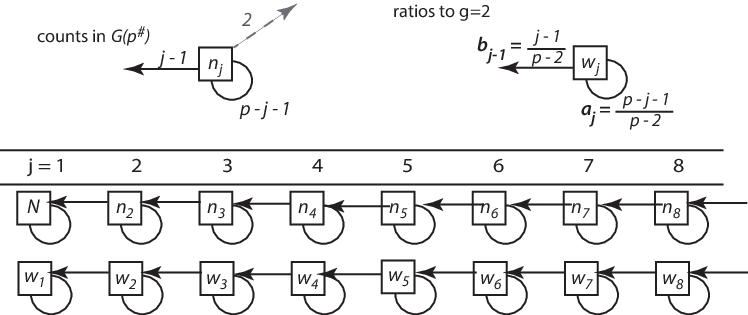
A direct corollary to Theorem 2.3 and Lemma 3.1 gives us an exact description of the growth of the populations of various constellations across all stages of Eratosthenes sieve. (Keep in mind that a gap is a constellation of length $1$ .)

Corollary 3.2.

If $s$ is any constellation in ${\mathcal{G}}({p_{k}}^{\#})$ of length $j$ and sum $g<2p_{k+1}$ , with $n_{s,j+1}({p_{k}}^{\#})$ driving terms of length $j+1$ in ${\mathcal{G}}({p_{k}}^{\#})$ , then

N_{s}({p_{k+1}}^{\#})=(p_{k+1}-j-1)\cdot N_{s}({p_{k}}^{\#})+1\cdot n_{s,j+1}({p_{k}}^{\#}).

From this corollary, we note that the coefficients for the population model do not depend on the constellation $s$ . The first-order growth of the population of every constellation $s$ of length $j$ and sum $g<2p_{k+1}$ is given by the factor $p_{k+1}-j-1$ . This is independent of the sequence of gaps within $s$ . As we have seen above, constellations may differ significantly in the populations of their driving terms.

Although the asymptotic growth of all constellations of length $j$ is equal, the initial conditions and driving terms are important. Brent [1] made analogous observations for single gaps ( $j=1$ ). His Table 2 indicates the importance of the lower-order effects in estimating relative occurrences of certain gaps.

3.2. Relative populations of $g=2,\;6,\;8,\;10$

What can we say about the relative populations of the gaps $g=2,\;6,\;8$ over later stages of the sieve? The population of every gap grows by a factor of $p-2$ . The populations differ by the presence of driving terms of various lengths and by the initial conditions.

We proceed by normalizing each population by the population of the gap $g=2$ . To compare the populations of any gap $g$ to the gap $2$ over later stages of the sieve, we take the ratio

(4)

w_{{g},{1}}({p}^{\#})=\frac{N_{g}({p}^{\#})}{N_{2}({p}^{\#})}.

Letting $n_{g,j}({p}^{\#})$ denote the number of all driving terms of sum $g$ and length $j$ in the cycle of gaps ${\mathcal{G}}({p}^{\#})$ , we can extend this definition to

w_{{g},{j}}({p}^{\#})=\frac{n_{g,j}({p}^{\#})}{N_{2}({p}^{\#})}.

These ratios for the gaps $g=6$ and $g=8$ are given by the $3$ -dimensional dynamic system:

$\displaystyle\left[\begin{array}[]{c}w_{{g},{1}}\\ w_{{g},{2}}\\ w_{{g},{3}}\end{array}\right]_{{p_{k+1}}^{\#}}$	$\displaystyle=$	$\displaystyle\left[\begin{array}[]{ccc}1&\frac{1}{p_{k+1}-2}&0\\ 0&\frac{p_{k+1}-3}{p_{k+1}-2}&\frac{2}{p_{k+1}-2}\\ 0&0&\frac{p_{k+1}-4}{p_{k+1}-2}\end{array}\right]\cdot\left[\begin{array}[]{c}w_{{g},{1}}\\ w_{{g},{2}}\\ w_{{g},{3}}\end{array}\right]_{{p_{k}}^{\#}}$
$\displaystyle{\rm or}$
$\displaystyle\left.\bar{w}_{{g}}\right\|_{{{p_{k+1}}^{\#}}}$	$\displaystyle=$	$\displaystyle\left.M_{{3}}\right\|_{{p_{k+1}}}\cdot\left.\bar{w}_{{g}}\right\|_{{{p_{k}}^{\#}}}$

with initial conditions

\begin{array}[]{ccc}\left.\bar{w}_{{6}}\right|_{{{5}^{\#}}}=\left[\begin{array}[]{c}2/3\\ 4/3\\ 0\end{array}\right],&\left.\bar{w}_{{8}}\right|_{{{5}^{\#}}}=\left[\begin{array}[]{c}0\\ 2/3\\ 1/3\end{array}\right]\end{array}

For this dynamic system, our attention turns to the $3\times 3$ system matrix $M_{3}(p)$ and its eigenstructure. Here the system matrix depends on the prime $p$ (but not on the gap $g$ ), so that as we iterate, we have to keep track of this dependence.

\left.\bar{w}_{{g}}\right|_{{{p_{k}}^{\#}}}=\left.M_{{3}}\right|_{{p_{k}}}\cdot\left.M_{{3}}\right|_{{p_{k-1}}}\cdots\left.M_{{3}}\right|_{{p_{1}}}\left.\bar{w}_{{g}}\right|_{{{p_{0}}^{\#}}}

A simple calculation shows that we are in luck. The eigenvalues of $M_{3}(p)$ depend on $p$ but the eigenvectors do not. We write the eigenstructure of $M_{3}(p)$ as

\left.M_{{3}}\right|_{{p}}=R_{3}\cdot\left.\Lambda_{3}\right|_{p}\cdot L_{3}

in which $\Lambda(p)$ is the diagonal matrix of eigenvalues, $R$ is the matrix of right eigenvectors, and $L$ is the matrix of left eigenvectors, such that $L\cdot R=I$ .

If it is true that the eigenvectors do not depend on $p$ , then the iterative system simplifies:

	$\displaystyle\left.\bar{w}_{{g}}\right\|_{{{p_{k}}^{\#}}}$	$\displaystyle=$	$\displaystyle\left.M_{{3}}\right\|_{{p_{k}}}\cdot\left.M_{{3}}\right\|_{{p_{k-1}}}\cdots\left.M_{{3}}\right\|_{{p_{1}}}\left.\bar{w}_{{g}}\right\|_{{{p_{0}}^{\#}}}$
		$\displaystyle=$	$\displaystyle R\cdot\left.\Lambda_{{3}}\right\|_{{p_{k}}}\cdot\left.\Lambda_{{3}}\right\|_{{p_{k-1}}}\cdots\left.\Lambda_{{3}}\right\|_{{p_{1}}}\cdot L\left.\bar{w}_{{g}}\right\|_{{{p_{0}}^{\#}}}$

Here the dependence on $p$ leads to a product of diagonal matrices. We exhibit the full eigenstructure for dimension $3$ , to confirm that the eigenvectors do not depend on $p$ , so that we can complete the calculations.

\begin{array}[]{rcccc}\left.M_{{3}}\right|_{{p}}&=&R_{3}&\left.\Lambda_{{3}}\right|_{{p}}&L_{3}\\ &=&\left[\begin{array}[]{rrr}1&-1&1\\ 0&1&-2\\ 0&0&1\end{array}\right]\cdot&\left[\begin{array}[]{rcc}1&0&0\\ 0&\frac{p-3}{p-2}&0\\ 0&0&\frac{p-4}{p-2}\end{array}\right]&\cdot\left[\begin{array}[]{rrr}1&1&1\\ 0&1&2\\ 0&0&1\end{array}\right]\end{array}

If we fix $p_{0}$ , then we can define $M^{k}_{3}=M_{3}(p_{k})\cdots M_{3}(p_{1})$ :

\begin{array}[]{rcccc}M^{k}_{3}&=&R_{3}&\left.\Lambda_{{3}}\right|_{{p_{k}}}\cdots\left.\Lambda_{{3}}\right|_{{p_{1}}}&L_{3}\\ &=&\left[\begin{array}[]{rrr}1&-1&1\\ 0&1&-2\\ 0&0&1\end{array}\right]\cdot&\left[\begin{array}[]{rcc}1&0&0\\ 0&\prod_{p_{1}}^{p_{k}}\frac{p-3}{p-2}&0\\ 0&0&\prod_{p_{1}}^{p_{k}}\frac{p-4}{p-2}\end{array}\right]&\cdot\left[\begin{array}[]{rrr}1&1&1\\ 0&1&2\\ 0&0&1\end{array}\right]\end{array}

Let $a_{2}^{k}=\prod_{p_{1}}^{p_{k}}\frac{p-3}{p-2}$ , and $a_{3}^{k}=\prod_{p_{1}}^{p_{k}}\frac{p-4}{p-2}$ .

So for any gap $g<2p_{1}$ that has driving terms of a maximum length of $3$ , once we know the initial populations in ${\mathcal{G}}({p_{0}}^{\#})$ , we can use the eigenstructure of $M^{k}_{3}$ to completely characterize the populations of $g$ and its driving terms in a very compact form. Starting with the initial conditions

\left.\bar{w}_{{g}}\right|_{{{p_{0}}^{\#}}}=\left[\begin{array}[]{c}w_{g,1}\\ w_{g,2}\\ w_{g,3}\end{array}\right]_{{p_{0}}^{\#}},

we apply the left eigenvectors $L_{3}$ to obtain the coordinates relative to the basis of right eigenvectors $R_{3}$ . After this transformation, we can apply the actions of the eigenvalues $\Lambda_{3}(p)$ directly to the individual right eigenvectors.

$\displaystyle\left.\bar{w}_{{g}}\right\|_{{{p_{k}}^{\#}}}$	$\displaystyle=$	$\displaystyle M^{k}_{3}\cdot\left.\bar{w}_{{g}}\right\|_{{{p_{0}}^{\#}}}$
	$\displaystyle=$	$\displaystyle R_{3}\cdot\left.\Lambda_{{3}}\right\|_{{p_{k}}}\cdots\left.\Lambda_{{3}}\right\|_{{p_{1}}}\cdot L_{3}\cdot\left.\bar{w}_{{g}}\right\|_{{p_{0}}}$
	$\displaystyle=$	$\displaystyle\left[\begin{array}[]{rrr}1&-1&1\\ 0&1&-2\\ 0&0&1\end{array}\right]\cdot\left[\begin{array}[]{rrr}1&0&0\\ 0&a_{2}^{k}&0\\ 0&0&a_{3}^{k}\end{array}\right]\cdot\left[\begin{array}[]{rrr}1&1&1\\ 0&1&2\\ 0&0&1\end{array}\right]\cdot\left[\begin{array}[]{c}w_{g,1}\\ w_{g,2}\\ w_{g,3}\end{array}\right]_{{p_{0}}^{\#}}$
	$\displaystyle=$	$\displaystyle\left[\begin{array}[]{rrr}1&-1&1\\ 0&1&-2\\ 0&0&1\end{array}\right]\cdot\left[\begin{array}[]{rrr}1&0&0\\ 0&a_{2}^{k}&0\\ 0&0&a_{3}^{k}\end{array}\right]\cdot\left[\begin{array}[]{r}w_{g,1}+w_{g,2}+w_{g,3}\\ w_{g,2}+2w_{g,3}\\ w_{g,3}\end{array}\right]_{{p_{0}}^{\#}}$
	$\displaystyle=$	$\displaystyle\left[\begin{array}[]{rrr}1&-1&1\\ 0&1&-2\\ 0&0&1\end{array}\right]\cdot\left[\begin{array}[]{r}w_{g,1}+w_{g,2}+w_{g,3}\\ a_{2}^{k}(w_{g,2}+2w_{g,3})\\ a_{3}^{k}\;w_{g,3}\end{array}\right]_{{p_{0}}^{\#}}$
	$\displaystyle=$	$\displaystyle\left[\begin{array}[]{r}(w_{g,1}+w_{g,2}+w_{g,3})-a_{2}^{k}(w_{g,2}+2w_{g,3})+a_{3}^{k}\;w_{g,3}\\ a_{2}^{k}(w_{g,2}+2w_{g,3})-2a_{3}^{k}\;w_{g,3}\\ a_{3}^{k}\;w_{g,3}\end{array}\right]_{{p_{0}}^{\#}}$

Right away we observe that the asymptotic ratio $w_{g,1}(\infty)$ of the gap $g$ to the gap $2$ is the sum of the initial ratios of all of $g$ ’s driving terms. We also observe that the ratio converges to the asymptotic value as quickly as $a_{2}^{k}\longrightarrow 0$ . While $a_{3}^{k}$ becomes small pretty quickly, the convergence of $a_{2}^{k}$ is slow. Figure 3 plots $a_{2}^{k}$ and $a_{3}^{k}$ for $p_{0}=13$ up to $p\approx 3\cdot 10^{15}$ .

Let us apply the above analysis to all of the gaps that satisfy the required conditions. Using $p_{0}=5$ , we observe in ${\mathcal{G}}({5}^{\#})=64242462$ that the smallest sum of a constellation of length $4$ is $12$ , for $s=2424$ . So we cannot apply the analysis to $g=12$ , but we can for the gaps $g=6,\;8,\;10$ .

${\mathcal{G}}({5}^{\#})=64242462$
$g$	$w_{g,1}({5}^{\#})$	$w_{g,2}({5}^{\#})$	$w_{g,3}({5}^{\#})$	$w_{g,1}(\infty)$
$6$	$2/3$	$4/3$	$0$	$2$
$8$	$0$	$2/3$	$1/3$	$1$
$10$	$0$	$2/3$	$2/3$	$4/3$

To obtain the asymptotic ratio $w_{g,1}(\infty)$ , we simply add together the initial ratios of all driving terms. These results tell us that as quickly as $a_{2}^{k}\longrightarrow 0$ , the number of occurrences of the gap $g=6$ in the cycle of gaps ${\mathcal{G}}({p}^{\#})$ for Eratosthenes sieve approaches double the number of gaps $g=2$ . Despite having driving terms of length two and of length three, the number of gaps $g=8$ approaches the number of gaps $g=2$ in later stages of the sieve, and the ratio of the number of gaps $g=10$ to the number of gaps $g=2$ approaches $4/3$ .

These are not probabilistic estimates. These ratios are based on the actual counts of the populations of these gaps and their driving terms across stages of Eratosthenes sieve.

4. First set of results on gaps and constellations for Eratosthenes sieve

Before developing the general dynamic system that describes the population of any gap $g=2k$ in the cycle of gaps, we pause to list the following results which we can already establish.

•

Twin Generators. The number of gaps $g=2$ in the cycle of gaps ${\mathcal{G}}({p_{k}}^{\#})$ is

$N_{2}({p_{k}}^{\#})=\prod_{q=3}^{p_{k}}(q-2).$

Proof: This is a direct application of Corollary 3.2.
•

Primorial conjecture for $6={3}^{\#}$ . From our work above on the $3$ -dimensional dynamic system, we have calculated the asymptotic ratio between the numbers of gaps $6={3}^{\#}$ and $2={2}^{\#}$ ,

$w_{6,1}(\infty)=\lim_{q\longrightarrow\infty}\frac{N_{{3}^{\#}}({q}^{\#})}{N_{{2}^{\#}}({q}^{\#})}=2$

But $2=\frac{3-1}{3-2}$ , which is the ratio of occurrences implied by Hardy and Littlewood’s Conjecture B.
•

ET Spikes. For gaps in the cycles of gaps,

$\lim\sup\frac{g_{i+1}}{g_{i}}=\infty\makebox[5.42003pt]{}{\rm and}\makebox[5.42003pt]{}\lim\inf\frac{g_{i+1}}{g_{i}}=0.$

In particular, for $g_{i}=2$ , the adjacent gaps $g_{i-1}$ and $g_{i+1}$ become arbitrarily large in later stages of the sieve.

Proof: This is a direct result of Theorem 2.3. Let $s_{k}=2\tilde{g}_{k}$ be the constellation of length two in ${\mathcal{G}}({p_{k}}^{\#})$ with first gap $2$ and second gap $\tilde{g}_{k}$ such that $\tilde{g}_{k}$ is the largest that occurs among all such constellations of length two.

$\tilde{g}_{k}=\max\left\{g\makebox[5.42003pt]{}:\makebox[5.42003pt]{}s=2g\;{\rm occurs\;in}\;{\mathcal{G}}({p_{k}}^{\#})\right\}$

In forming ${\mathcal{G}}({p_{k+1}}^{\#})$ the closure to the right of $\tilde{g}_{k}$ occurs exactly once. Thus $\tilde{g}_{k+1}>\tilde{g}_{k}$ , and we have our result for $\limsup$ .

By symmetry of ${\mathcal{G}}({p}^{\#})$ the constellation $\tilde{g}_{k}2$ also occurs, and we thereby have our result for $\liminf$ .
•

ET Superlinear growth. For every $k>1$ there is a cycle of gaps ${\mathcal{G}}({p}^{\#})$ with a constellation of $k$ consecutive gaps such that

$g_{n+1}<g_{n+2}<\cdots<g_{n+k}.$

This constellation persists across all subsequent stages of the sieve, and its population increases by the factor $p-k-1$ at each stage.

Proof: In the middle of the cycle of gaps ${\mathcal{G}}({p_{i}}^{\#})$ there occurs the constellation

$\tilde{s}_{j}=2^{j}\;2^{j-1}\ldots 842\;4\;248\ldots 2^{j-1}\;2^{j}$

in which $j$ is the smallest number such that $2^{j+1}>p_{i+1}$ . For a given $k$ , we take $p_{i}$ large enough so that $j>k$ . Then the right half of $\tilde{s}_{j}$ is the desired constellation, and it satisfies the condition $|s|=2^{j+1}-2<2p_{i+1}.$

The persistence of the constellation and the growth of its population by the factor $p-k-1$ is given by Corollary 3.2.
•

ET Superlinear decay. For every $k>1$ there is a cycle of gaps ${\mathcal{G}}({p}^{\#})$ with a constellation of $k$ consecutive gaps such that

$g_{n+1}>g_{n+2}>\cdots>g_{n+k}.$

This constellation persists across all subsequent stages of the sieve, and its population increases by the factor $p-k-1$ at each stage. Proof: The desired constellation is the left half of $\tilde{s}_{j}$ .

5. A model for populations across iterations of the sieve

We now identify a discrete dynamic system that provides exact counts of a gap and its driving terms. These raw counts grow superexponentially, and so to better understand their behavior we take the ratio of a raw count to the number of gaps $g=2$ at each stage of the sieve. In the work above we created and examined this dynamic system for driving terms up to length $3$ . Here we generalize this approach by considering driving terms up to length $J$ , for any $J$ .

Fix a sufficiently large size $J$ . For any gap $g$ that has driving terms of lengths up to $j$ , with $j\leq J$ , we form a vector of initial values $\left.\bar{w}\right|_{p_{0}}$ , whose $i^{\rm th}$ entry is the ratio of the number of driving terms for $g$ of length $i$ in ${\mathcal{G}}({p_{0}}^{\#})$ to the number of gaps $2$ in this cycle of gaps.

Generalizing our work for $J=3$ above, we model the population of the gap $g$ and its driving terms across stages of Eratosthenes sieve as a discrete dynamic system.

	$\displaystyle\left.\bar{w}\right\|_{{p_{k}}^{\#}}$	$\displaystyle=$	$\displaystyle M_{J}(p_{k})\cdot\left.\bar{w}\right\|_{{p_{k-1}}^{\#}}$
		$\displaystyle=$	$\displaystyle\left[\begin{array}[]{cccccc}1&b_{1}&0&\cdots&&0\\ 0&a_{2}&b_{2}&\ddots&&0\\ &0&a_{3}&b_{3}&\ddots&0\\ \vdots&&\ddots&\ddots&\ddots&0\\ 0&&\cdots&&a_{J-1}&b_{J-1}\\ 0&&\cdots&&0&a_{J}\end{array}\right]_{p_{k}}\cdot\left.\bar{w}\right\|_{{p_{k-1}}^{\#}}$

in which

(11)

a_{j}(p)=\frac{p-j-1}{p-2}\makebox[10.84006pt]{}{\rm and}\makebox[10.84006pt]{}b_{j}(p)=\frac{j}{p-2}.

Iterating this discrete dynamic system from the initial conditions at $p_{0}$ up through $p_{k}$ , we have

	$\displaystyle\left.\bar{w}\right\|_{{p_{k}}^{\#}}$	$\displaystyle=$	$\displaystyle\left.M_{J}\right\|_{p_{k}}\cdot\left.\bar{w}\right\|_{{p_{k-1}}^{\#}}$
		$\displaystyle=$	$\displaystyle M_{J}^{k}\cdot\left.\bar{w}\right\|_{{p_{0}}^{\#}}$

The matrix $M_{J}$ does not depend on the gap $g$ . It does depend on the prime $p_{k}$ , and we use the exponential notation $M_{J}^{k}$ to indicate the product of the $M$ ’s over the indicated range of primes.

That $M_{J}$ does not depend on the gap $g$ is interesting. This means that the recursion treats all gaps fairly. The recursion itself is not biased toward certain gaps or constellations. Once a gap has driving terms in ${\mathcal{G}}({p}^{\#})$ , the populations across all further stages of the sieve are completely determined.

$M_{J}^{k}$ applies to all constellations whose driving terms have length $j\leq J$ ; and we continue to use the exponential notation to denote the product over the sequence of primes from $p_{1}$ to $p_{k}$ : e.g.

M_{J}^{k}=\left.M_{{J}}\right|_{{p_{k}}}\cdot\left.M_{{J}}\right|_{{p_{k-1}}}\cdots\left.M_{{J}}\right|_{{p_{1}}}.

With $M_{J}^{k}$ we can calculate the ratios $w_{{g},{j}}(p_{k})$ for the complete system of driving terms, relative to the population of the gap $2$ , for the cycle of gaps ${\mathcal{G}}({p_{k}}^{\#})$ (here, $p_{k}$ is the $k^{\rm th}$ prime after $p_{0}$ ). With $J=3$ we calculated above the ratios for $g=6,\;8,\;10.$ For $g=12$ we need $J=4$ , and for $g=30$ , we need $J=8$ .

Fortunately, we can completely describe the eigenstructure for $\left.M_{J}\right|_{p}$ , and even better – the eigenvectors for $M_{J}$ do not depend on the prime $p$ . This means that we can use the eigenstructure to provide a simple description of the behavior of this iterative system as $k\longrightarrow\infty$ .

5.1. Eigenstructure of $M_{J}$

We list the eigenvalues, the left eigenvectors and the right eigenvectors for $M_{J}$ , writing these in the product form

M_{J}=R\cdot\Lambda\cdot L

with $LR=I$ . For the general system $M_{J}$ , the upper triangular entries of $R$ and $L$ are binomial coefficients, with those in $R$ of alternating sign; and the eigenvalues are the $a_{j}$ defined in Equation 11 above.

$\displaystyle R_{ij}$	$\displaystyle=$	$\displaystyle\left\{\begin{array}[]{cl}(-1)^{i+j}\left(\begin{array}[]{c}{j-1}\\ {i-1}\end{array}\right)&{\rm if}\;i\leq j\\ &\\ 0&{\rm if}\;i>j\end{array}\right.$
$\displaystyle\Lambda$	$\displaystyle=$	$\displaystyle{\rm diag}(1,a_{2},\ldots,a_{J})$
$\displaystyle L_{ij}$	$\displaystyle=$	$\displaystyle\left\{\begin{array}[]{ll}\left(\begin{array}[]{c}{j-1}\\ {i-1}\end{array}\right)&{\rm if}\;i\leq j\\ &\\ 0&{\rm if}\;i>j\end{array}\right.$

For any vector $\bar{w}$ , multiplication by the left eigenvectors (the rows of $L$ ) yields the coefficients for expressing this vector of initial conditions over the basis given by the right eigenvectors (the columns of $R$ ):

\bar{w}=(L_{1\cdot}\bar{w})R_{\cdot 1}+\cdots+(L_{J\cdot}\bar{w})R_{\cdot J}

Lemma 5.1.

Let $g$ be a gap and $p_{0}$ a prime such that $g<2p_{1}$ . In ${\mathcal{G}}({p_{0}}^{\#})$ let the initial ratios for $g$ and its driving terms be given by $\left.\bar{w}_{{g}}\right|_{{{p_{0}}^{\#}}}$ . Then the ratio of occurrences of this gap $g$ to occurrences of the gap $2$ in ${\mathcal{G}}({p}^{\#})$ as $p\longrightarrow\infty$ converges to the sum of the initial ratios across the gap $g$ and all its driving terms:

w_{{g},{1}}(\infty)=L_{1\cdot}\left.\bar{w}_{{g}}\right|_{{{p_{0}}^{\#}}}=\sum_{j}\left.w_{{g},{j}}\right|_{{p_{0}}^{\#}}.

Proof.

Let $g$ have driving terms up to length $J$ . Then the ratios $\left.\bar{w}_{{g}}\right|_{{{p}^{\#}}}$ are given by the iterative linear system

\left.\bar{w}_{{g}}\right|_{{{p_{k}}^{\#}}}=M_{J}^{k}\cdot\left.\bar{w}_{{g}}\right|_{{{p_{0}}^{\#}}}.

From the eigenstructure of $M_{J}$ , we have

\left.\bar{w}_{{g}}\right|_{{{p_{0}}^{\#}}}=(L_{1}\left.\bar{w}_{{g}}\right|_{{{p_{0}}^{\#}}})R_{1}+(L_{2}\left.\bar{w}_{{g}}\right|_{{{p_{0}}^{\#}}})R_{2}+\cdots+(L_{J}\left.\bar{w}_{{g}}\right|_{{{p_{0}}^{\#}}})R_{J},

and so

(16)		$\displaystyle M_{J}^{k}\left.\bar{w}_{{g}}\right\|_{{{p_{0}}^{\#}}}$	$\displaystyle=$	$\displaystyle(L_{1}\left.\bar{w}_{{g}}\right\|_{{{p_{0}}^{\#}}})R_{1}+a_{2}^{k}(L_{2}\left.\bar{w}_{{g}}\right\|_{{{p_{0}}^{\#}}})R_{2}+\cdots$
(16)				$\displaystyle\cdots+a_{J}^{k}(L_{J}\left.\bar{w}_{{g}}\right\|_{{{p_{0}}^{\#}}})R_{J}.$

We note that $L_{1\cdot}=[1\cdots 1]$ , $\lambda_{1}=1$ , and $R_{\cdot 1}=e_{1}$ ; that the other eigenvalues $a_{j}^{k}\longrightarrow 0$ with $a_{j}^{k}>a_{j+1}^{k}$ . Thus as $k\longrightarrow\infty$ the terms on the righthand side decay to $0$ except for the first term, establishing the result. ∎

With Lemma 5.1 and the initial values in ${\mathcal{G}}({13}^{\#})$ in Table 2, we can calculate the asymptotic ratios of the occurrences of the gaps $g=6,8,\ldots,32$ to the gap $g=2$ .

Values of $a_{j}^{k}$ at $p_{k}=999,999,999,989$ for $p_{0}=13$
	$a_{2}^{k}=0.10206751799779$
	$a_{3}^{k}=0.01019996897567$
$a_{j}^{k}=\prod_{q=17}^{p_{k}}\frac{q-j-1}{q-2}$	$a_{4}^{k}=0.00099592269918$
	$a_{5}^{k}=0.00009477093531$
	$a_{6}^{k}=0.00000876214163$
	$a_{7}^{k}=0.00000078408120$
	$a_{8}^{k}=0.00000006757562$
	$a_{9}^{k}=0.00000000557284$

Table 1. Calculated values of the eigenvalues

a_{j}^{k}

up to

p_{k}\approx 10^{12}

. If we use initial conditions from

{\mathcal{G}}({13}^{\#})

, then

p_{0}=13

and the products start with

p_{1}=17

From the calculated values in Table 1, we see the decay of the $a_{j}^{k}$ toward $0$ , but $a_{2}^{k}$ and $a_{3}^{k}$ are still making significant contributions when $p_{k}\approx 10^{12}$ .

In Table 2 we used $p_{0}=13$ for our initial conditions since the prime $p=13$ is the first prime for which the conditions of Corollary 3.2 are satisifed for the next primorial $g={5}^{\#}=30$ .

gap	$n_{g,j}(13)$ : driving terms of length $j$ in ${\mathcal{G}}({13}^{\#})$
$g$	$j=1$	$2$	$3$	$4$	$5$	$6$	$7$	$8$	$9$
$\scriptstyle 2,\;4$	$\scriptstyle 1485$
$\scriptstyle 6$	$\scriptstyle 1690$	$\scriptstyle 1280$
$\scriptstyle 8$	$\scriptstyle 394$	$\scriptstyle 902$	$\scriptstyle 189$
$\scriptstyle 10$	$\scriptstyle 438$	$\scriptstyle 1164$	$\scriptstyle 378$
$\scriptstyle 12$	$\scriptstyle 188$	$\scriptstyle 1276$	$\scriptstyle 1314$	$\scriptstyle 192$
$\scriptstyle 14$	$\scriptstyle 58$	$\scriptstyle 536$	$\scriptstyle 900$	$\scriptstyle 288$
$\scriptstyle 16$	$\scriptstyle 12$	$\scriptstyle 252$	$\scriptstyle 750$	$\scriptstyle 436$	$\scriptstyle 35$
$\scriptstyle 18$	$\scriptstyle 8$	$\scriptstyle 256$	$\scriptstyle 1224$	$\scriptstyle 1272$	$\scriptstyle 210$
$\scriptstyle 20$	$\scriptstyle 0$	$\scriptstyle 24$	$\scriptstyle 348$	$\scriptstyle 960$	$\scriptstyle 600$	$\scriptstyle 48$
$\scriptstyle 22$	$\scriptstyle 2$	$\scriptstyle 48$	$\scriptstyle 312$	$\scriptstyle 784$	$\scriptstyle 504$
$\scriptstyle 24$	$\scriptstyle 0$	$\scriptstyle 20$	$\scriptstyle 258$	$\scriptstyle 928$	$\scriptstyle 1260$	$\scriptstyle 504$
$\scriptstyle 26$	$\scriptstyle 0$	$\scriptstyle 2$	$\scriptstyle 40$	$\scriptstyle 322$	$\scriptstyle 724$	$\scriptstyle 448$	$\scriptstyle 84$
$\scriptstyle 28$	$\scriptstyle 0$	$\scriptstyle 0$	$\scriptstyle 36$	$\scriptstyle 344$	$\scriptstyle 794$	$\scriptstyle 528$	$\scriptstyle 80$
$\scriptstyle 30$	$\scriptstyle 0$	$\scriptstyle 0$	$\scriptstyle 10$	$\scriptstyle 194$	$\scriptstyle 1066$	$\scriptstyle 1784$	$\scriptstyle 816$	$\scriptstyle 90$
$\scriptstyle 32$	$\scriptstyle 0$	$\scriptstyle 0$	$\scriptstyle 0$	$\scriptstyle 12$	$\scriptstyle 200$	$\scriptstyle 558$	$\scriptstyle 523$	$\scriptstyle 172$	$\scriptstyle 20$

Table 2. For small gaps

g

, this table lists the number of gaps and driving terms of length

j

that occur in the cycle of gaps

{\mathcal{G}}({13}^{\#})

. We can use these as initial conditions for the population model in Equation 16 of size

J\leq 9

Applying Lemma 5.1 to the initial conditions for $p_{0}=13$ in Table 2, as $p_{k}\longrightarrow\infty$ , the following ratios describe the relative frequency of occurrence of these gaps in Eratosthenes sieve:

ratio $w_{g,1}(\infty)$ :	gaps $g$ with this ratio
$1$ :	$2,\;4,\;8,\;16,\;32$
$1.\overline{09}$ :	$26$
$1.\bar{1}$ :	$22$
$1.2$ :	$14,\;28$
$1.\bar{3}$ :	$10,\;20$
$2$ :	$6,\;12,\;18,\;24$
$2.\bar{6}$ :	$30$

This table begins to suggest that the ratios implied by Hardy and Littlewood’s Conjecture B may hold true in Eratosthenes sieve.

The ratios discussed in this paper give the exact values of the relative frequencies of various gaps and constellations as compared to the number of gaps $2$ at each stage of Eratosthenes sieve. For gaps between primes, if the closures are at all fair as the sieving process continues, then these ratios in stages of the sieve should also be good indicators of the relative occurrence of these gaps and constellations among primes.

5.2. Primorial $g={5}^{\#}=30$ .

We also see that the primorial $g={5}^{\#}=30$ eventually becomes more numerous than $g={3}^{\#}=6$ . However, if we apply the expansion of the higher order terms

(17)		$\displaystyle\left.\bar{w}_{{g}}\right\|_{{{p_{k}}^{\#}}}$	$\displaystyle=$	$\displaystyle M_{J}^{k}\left.\bar{w}_{{g}}\right\|_{{{p_{0}}^{\#}}}$
(17)			$\displaystyle=$	$\displaystyle(L_{1}\left.\bar{w}_{{g}}\right\|_{{{p_{0}}^{\#}}})R_{1}+a_{2}^{k}(L_{2}\left.\bar{w}_{{g}}\right\|_{{{p_{0}}^{\#}}})R_{2}+\cdots+a_{J}^{k}(L_{J}\left.\bar{w}_{{g}}\right\|_{{{p_{0}}^{\#}}})R_{J}$

to the initial conditions for $p_{0}=13$ , using the $a_{j}^{k}$ as tabulated for $\hat{p}=999,999,999,989$ , we calculate that for $p_{k}\approx 10^{12}$

\left.\bar{w}_{{6}}\right|_{{{\hat{p}}^{\#}}}\approx 1.912\makebox[10.84006pt]{}{\rm and}\makebox[10.84006pt]{}\left.\bar{w}_{{30}}\right|_{{{\hat{p}}^{\#}}}\approx 1.579.

The convergence to the asymptotic values is very slow, due primarily to the slow decay of $a_{2}^{k}$ .

For what $p$ will $\left.\bar{w}_{{30}}\right|_{{{p}^{\#}}}>\left.\bar{w}_{{6}}\right|_{{{p}^{\#}}}$ ? That is, when will the gap $30$ be more numerous in Eratosthenes sieve than the gap $6$ ? To estimate this, we examine the first coordinate across the terms in Equation 17. The first coordinates of the $R$ ’s are $1$ ’s of alternating sign, and so we have

\left.\bar{w}_{{g}}\right|_{{{p}^{\#}}}=(L_{1}\left.\bar{w}_{{g}}\right|_{{{p_{0}}^{\#}}})-a_{2}^{k}(L_{2}\left.\bar{w}_{{g}}\right|_{{{p_{0}}^{\#}}})+\cdots+(-1)^{J+1}a_{J}^{k}(L_{J}\left.\bar{w}_{{g}}\right|_{{{p_{0}}^{\#}}}).

To estimate where $\left.\bar{w}_{{30}}\right|_{{{p}^{\#}}}-\left.\bar{w}_{{6}}\right|_{{{p}^{\#}}}>0$ , we make the rough approximation that for $p_{k}>>j$ ,

a_{j}^{k}\approx(a_{2}^{k})^{j-1}

and solve for the parameter $a_{2}^{k}$ . Using the data from $p_{0}=13$ , we see that $\left.\bar{w}_{{30}}\right|_{{{p}^{\#}}}>\left.\bar{w}_{{6}}\right|_{{{p}^{\#}}}$ , that is, that the gaps $30$ will finally be more numerous in Eratosthenes sieve than the gaps $6$ , when $a_{2}^{k}<0.06275$ .

For $p_{0}=13$ , when $p_{k}\approx 10^{12}$ the parameter $a_{2}^{k}\approx 0.1$ , and when $p_{k}\approx 10^{15}$ the parameter $a_{2}^{k}\approx 0.08$ . The decay of $a_{2}^{k}$ is so slow that there will still be fewer gaps $30$ than gaps $6$ in Eratosthenes sieve when $p\approx 10^{15}$ .

6. Polignac’s conjecture and
Hardy & Littlewood’s Conjecture B

At this point, here is what we know about the population of a gap $g$ through the cycles of gaps ${\mathcal{G}}({p}^{\#})$ in Eratosthenes sieve. We need $p_{0}$ such that conditions of Corollary 3.2 hold, in particular the condition $g<2p_{1}$ . Then we need $J$ such that no constellation of length $J+1$ has sum equal to $g$ . This is the size of system we need to consider, to apply the dynamic system of Equation (16) to $g$ and its driving terms. For a given $g$ , once we have $p_{0}$ and $J$ , from ${\mathcal{G}}({p_{0}}^{\#})$ we can obtain counts of driving terms for $g$ from length $1$ to $J$ to create the initial conditions $w_{g}({p_{0}}^{\#})$ , and we can apply the model directly or through its eigenstructure, to obtain the exact populations of $g$ and its driving terms through the all further stages of Eratosthenes sieve.

Our progress along this line of increasing $p_{0}$ and $J$ is complicated primarily by our having to construct ${\mathcal{G}}({p_{0}}^{\#})$ . This cycle of gaps contains $\phi({p_{0}}^{\#})$ elements, which grows unmanageably large. If we have ${\mathcal{G}}({p_{0}}^{\#})$ , then for every gap $g<2p_{1}$ we can enumerate the driving terms of various lengths. We take the maximum such length as $J$ .

In this section we introduce an alternate way to obtain initial conditions for any gap $g$ , sufficient to apply Lemma 5.1.

As an analogue to Polignac’s conjecture, we show that for any even number $2n$ , the gap $g=2n$ or its driving terms occur at some stage of Eratosthenes sieve, and we show that although we can’t apply the complete dynamic system, we do have enough information to get the asymptotic result from Lemma 5.1.

Polignac’s Conjecture: For any even number $2n$ , there are infinitely many prime pairs $p_{j}$ and $p_{j+1}$ such the difference $p_{j+1}-p_{j}=2n$ .

In Theorem 6.5 below we establish an analogue of Polignac’s conjecture for Eratosthenes sieve, that for any number $2n$ the gap $g=2n$ occurs infinitely often in Eratosthenes sieve, and the ratio of occurrences of this gap to the gap $2$ approaches the ratio implied by Hardy & Littlewood’s Conjecture B:

w_{g,1}(\infty)=\lim_{p\rightarrow\infty}\frac{N_{g}({p}^{\#})}{N_{2}({p}^{\#})}=\prod_{q>2,\;q|g}\frac{q-1}{q-2}.

To obtain this result, we first consider ${\mathbb{Z}}\bmod Q$ and its cycle of gaps ${\mathcal{G}}(Q)$ , in which $Q$ is the product of the prime divisors of $2n$ . We then bring this back into Eratosthenes sieve by filling in the primes missing from $Q$ to obtain a primorial ${p}^{\#}$ .

Once we are working with ${\mathcal{G}}({p}^{\#})$ , the condition $g<2p_{k+1}$ may still prevent us from applying Corollary 3.2. However, we are able to show that we have enough information to apply Lemma 5.1 under the construction we are using.

6.1. General recursion on cycles of gaps

We need to develop a more general form of the recursion on cycles of gaps, one that applies to creating ${\mathcal{G}}(qN)$ from ${\mathcal{G}}(N)$ for any prime $q$ and number $N$ . We also need a variant of Lemma 3.1 that does not require the condition $g<2p_{k+1}$ .

Let ${\mathcal{G}}(N)$ denote the cycle of gaps among the generators in ${\mathbb{Z}}\bmod N$ , with the first gap being that between $1$ and the next generator. There are $\phi(N)$ gaps in ${\mathcal{G}}(N)$ that sum to $N$ . In our work in the preceding sections, we focused on Eratosthenes sieve, in which $N={p}^{\#}$ , the primorials.

There is a one-to-one correspondence between generators of ${\mathbb{Z}}\bmod N$ and the gaps in ${\mathcal{G}}(N)$ . Let

{\mathcal{G}}(N)=g_{1}\;g_{2}\;\ldots g_{\phi(N)}.

Then for $k<\phi(N)$ , $g_{k}$ corresponds to the generator $\gamma=1+\sum_{j=1}^{k}g_{j}$ , and since $\sum_{j=1}^{\phi(N)}=N$ , the generator $1$ corresponds to $g_{\phi(N)}$ . Moreover, since $1$ and $N-1$ are always generators, $g_{\phi(N)}=2$ . For any generator $\gamma$ , $N-\gamma$ is also a generator, which implies that except for the final $2$ , ${\mathcal{G}}(N)$ is symmetric. As a convention, we write the cycles with the first gap being from $1$ to the next generator.

We build ${\mathcal{G}}(N)$ for any $N$ by introducing one prime factor at a time.

Lemma 6.1.

Given ${\mathcal{G}}(N)$ , for a prime $q$ we construct ${\mathcal{G}}(qN)$ as follows:

a)

if $q\mid N$ , then we concatenate $q$ copies of $N$ ,

${\mathcal{G}}(qN)=\underbrace{{\mathcal{G}}(N)\cdots{\mathcal{G}}(N)}_{q\makebox[5.42003pt]{}{\rm copies}}$
b)
if $q\not|N$ , then we build ${\mathcal{G}}(qN)$ in three steps:
1. R1
  
  Concatenate $q$ copies of ${\mathcal{G}}(N)$ ;
2. R2
  
  Close at $q$ ;
3. R3
  
  Close as indicated by the element-wise product $q*{\mathcal{G}}(N)$ .

Proof.

A number $\gamma$ in ${\mathbb{Z}}\bmod N$ is a generator iff $\gcd(\gamma,N)=1$ .

a)

Assume $q|N$ . Since $\gcd(\gamma,N)=1$ , we know that $q\not|\gamma$ .

For $j=0,1,\ldots,q-1$ , we have

$\gcd(\gamma+jN,qN)=\gcd(\gamma,qN)=\gcd(\gamma,N)=1.$

Thus $\gcd(\gamma,N)=1$ iff $\gcd(\gamma+jN,qN)=1$ , and so the generators of ${\mathbb{Z}}\bmod qN$ have the form $\gamma+jN$ , and the gaps take the indicated form.
b)

If $q\not|N$ then we first create a set of candidate generators for ${\mathbb{Z}}\bmod qN$ , by considering the set

$\left\{{\gamma+jN\makebox[5.42003pt]{}:\makebox[5.42003pt]{}\gcd(\gamma,N)=1,\makebox[5.42003pt]{}j=0,\ldots,q-1}\right\}.$

For gaps, this is the equivalent of step R1, concatenating $q$ copies of ${\mathcal{G}}(N)$ . The only prime divisor we have not accounted for is $q$ ; if $\gcd(\gamma+jN,q)=1$ , then this candidate $\gamma+jN$ is a generator of ${\mathbb{Z}}\bmod qN$ . So we have to remove $q$ and its multiples from among the candidates.

We first close the gaps at $q$ itself. We index the gaps in the $q$ concatenated copies of ${\mathcal{G}}(N)$ :

$g_{1}g_{2}\ldots g_{\phi(N)}\ldots g_{q\cdot\phi(N)}.$

Recalling that the first gap $g_{1}$ is the gap between the generator $1$ and the next smallest generator in ${\mathbb{Z}}\bmod N$ , the candidate generators are the running totals $\gamma_{j}=1+\sum_{i=1}^{j-1}g_{i}$ . We take the $j$ for which $\gamma_{j}=q$ , and removing $q$ from the list of candidate generators corresponds to replacing the gaps $g_{j-1}$ and $g_{j}$ with the sum $g_{j-1}+g_{j}$ . This completes step R2 in the construction.

To remove the remaining multiples of $q$ from among the candidate generators, we note that any multiples of $q$ that share a prime factor with $N$ have already been removed. We need only consider multiples of $q$ that are relatively prime to $N$ ; that is, we only need to remove $q\gamma_{j}$ for each generator $\gamma_{j}$ of ${\mathbb{Z}}\bmod N$ by closing the corresponding gaps.

We can perform these closures by working directly with the cycle of gaps ${\mathcal{G}}(N)$ . Since $q\gamma_{i+1}-q\gamma_{i}=qg_{i}$ , we can go from one closure to the next by tallying the running sum from the current closure until that running sum equals $qg_{i}$ . Technically, we create a series of indices beginning with $i_{0}=j$ such that $\gamma_{j}=q$ , and thereafter $i_{k}=j$ for which $\gamma_{j}-\gamma_{i_{k-1}}=q\cdot g_{k}$ . To cover the cycle of gaps under construction, which consists initially of $q$ copies of ${\mathcal{G}}(N)$ , $k$ runs only from $0$ to $\phi(N)$ . We note that the last interval wraps around the end of the cycle and back to $i_{0}$ : $i_{\phi(N)}=i_{0}$ .

∎

Theorem 6.2.

In step R3 of Lemma 6.1, each possible closure in ${\mathcal{G}}(N)$ occurs exactly once in constructing ${\mathcal{G}}(qN)$ .

Proof.

Consider each gap $g$ in ${\mathcal{G}}(N)$ . Since $q\not|N$ , $N\bmod q\neq 0$ . Under step R1 of the construction, $g$ has $q$ images. Let the generator corresponding to $g$ be $\gamma$ . Then the generators corresponding to the images of $g$ under step R1 is the set:

\left\{\gamma+jN\makebox[5.42003pt]{}:\makebox[5.42003pt]{}j=0,\ldots,q-1\right\}.

Since $N\bmod q\neq 0$ , there is exactly one $j$ for which $(\gamma+jN)\bmod q=0$ . For this gap $g$ , a closure in R2 and R3 occurs once and only once, at the image corresponding to the indicated value of $j$ . ∎

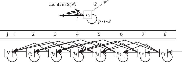
Corollary 6.3.

Let $g$ be a gap. If for the prime $q$ , $q\not|g$ , then

\sum w_{{g},{j}}(qN)=\sum w_{{g},{j}}(N).

Proof.

Consider a driving term $s$ for $g$ , of length $j$ in ${\mathcal{G}}(N)$ . In constructing ${\mathcal{G}}(qN)$ , we initially create $q$ copies of $s$ .

If $q|N$ , then the construction is complete. For each driving term for $g$ in ${\mathcal{G}}(N)$ we have $q$ copies, and so $n_{g,j}(qN)=q\cdot n_{g,j}(N).$ However, we also have $q$ copies of every gap $2$ in ${\mathcal{G}}(N)$ , $n_{2,1}(qN)=q\cdot n_{2,1}(N)$ . Thus $w_{{g},{j}}(qN)=w_{{g},{j}}(N)$ , and we have equality for each length $j$ , and so the result about the sum is immediate.

If $q\not|N$ , then in step R1 we create $q$ copies of $s$ . In steps R2 and R3, each of the possible closures in $s$ occurs once, distributed among the $q$ copies of $s$ . The $j-1$ closures interior to $s$ change the lengths of some of the driving terms but don’t change the sum, and the result is still a driving term for $g$ . Only the two exterior closures, one at each end of $s$ , change the sum and thereby remove the copy from being a driving term for $g$ . Since $q\not|g$ , these two exterior closures occur in separate copies of $s$ . See Figure 4.

If the condition $g<2p_{k+1}$ applies, then each of the closures occur in a separate copy of $s$ , and we can use the full dynamic system of Corollary 3.2. For the current result we do not know that the closures necessarily occur in distinct copies of $s$ , and so we can’t be certain of the lengths of the resulting constellations.

However, we do know that of the $q$ copies of $s$ , two are eliminated as driving terms and $q-2$ remain as driving terms of various lengths.

\sum_{j}n_{g,j}(qN)=(q-2)\sum_{j}n_{g,j}(N).

Since $n_{2,1}(qN)=(q-2)n_{2,1}(N)$ , the ratios are preserved

\sum_{j}w_{{g},{j}}(qN)=\sum_{j}w_{{g},{j}}(N).

∎

By combining the preceding Corollary 6.3 with Lemma 5.1, we immediately obtain the following result, that for any gap $g$ , if we look at its largest prime factor $\bar{q}$ , then we can calculate the asymptotic ratios from ${\mathcal{G}}({\bar{q}}^{\#})$ .

Corollary 6.4.

Let $g=2n$ be a gap, and let $\bar{q}$ be the largest prime factor of $g$ . Then

w_{{g},{1}}(\infty)=\sum w_{{g},{j}}({\bar{q}}^{\#}).

Proof.

For all primes $p>\bar{q}$ , by Corollary 6.3

\sum w_{{g},{j}}({p}^{\#})=\sum w_{{g},{j}}({\bar{q}}^{\#}),

so once we reach ${\mathcal{G}}({\bar{q}}^{\#})$ , we continue through additional stages of the sieve if necessary until the condition $g<2p_{1}$ is satisfied, but the ratios remain unchanged during this formality. So the result from Lemma 5.1 can be obtained from the ratios determined in ${\mathcal{G}}({\bar{q}}^{\#})$ . ∎

6.2. Polignac’s conjecture for Eratosthenes sieve

We establish an equivalent of Polignac’s conjecture for Eratosthenes sieve.

Theorem 6.5.

For every $n>0$ , the gap $g=2n$ occurs infinitely often in Eratosthenes sieve, and the ratio of the number of occurrences of $g=2n$ to the number of $2$ ’s converges asymptotically to

w_{{2n},{1}}(\infty)=\prod_{q>2,\;q|n}\frac{q-1}{q-2}.

We establish this result in two steps. First we find a stage of Eratosthenes sieve in which the gap $g=2n$ has driving terms. Once we can enumerate the driving terms for $g$ in this initial stage of Eratosthenes sieve, we can establish the asymptotic ratio of gaps $g=2n$ to the gaps $g=2$ as the sieve continues.

Lemma 6.6.

Let $g=2n$ be given. Let $Q$ be the product of the primes dividing $2n$ , including $2$ .

Q=\prod_{q|2n}q.

Finally, let $\bar{q}$ be the largest prime factor in $Q$ .

Then in ${\mathcal{G}}({\bar{q}}^{\#})$ the gap $g$ has driving terms, the total number of which satisfies

\sum_{j}n_{g,j}({\bar{q}}^{\#})=\phi(Q)\cdot\prod_{p<\bar{q},\;p\;\nmid\;Q}(p-2).

Proof.

Let $n_{1}=2n/Q$ . By Lemma 6.1 the cycle of gaps ${\mathcal{G}}(2n)$ consists of $n_{1}$ concatenated copies of ${\mathcal{G}}(Q)$ . In ${\mathcal{G}}(Q)$ , there are $\phi(Q)$ driving terms for the gap $g=2n$ . To see this, start at any gap in ${\mathcal{G}}(Q)$ and proceed through the cycle $n_{1}$ times. The length of each of these driving terms is initially $n_{1}\cdot\phi(Q)$ .

We now want to bring this back into Eratosthenes sieve.

Let $Q_{0}=Q$ , and let $p_{1},\ldots,p_{k}$ be the prime factors of ${\bar{q}}^{\#}/Q$ . For $i=1,\ldots,k$ , let $Q_{i}=p_{i}\cdot Q_{i-1}$ , with $Q_{k}={\bar{q}}^{\#}$ . In forming ${\mathcal{G}}(Q_{i})$ from ${\mathcal{G}}(Q_{i-1})$ , we apply Corollary 6.3. Since $p_{i}\not|g$ , we have

\sum_{j=1}^{J}n_{2n,j}(Q_{i})=(p_{i}-2)\cdot\sum_{j=1}^{J}n_{2n,j}(Q_{i-1})

Thus at $p_{k}$ we have

	$\displaystyle\sum_{j=1}^{J}n_{2n,j}({\bar{q}}^{\#})$	$\displaystyle=$	$\displaystyle\sum_{j=1}^{J}n_{2n,j}(Q_{k})\makebox[5.42003pt]{}=\makebox[5.42003pt]{}(p_{k}-2)\cdot\sum_{j=1}^{J}n_{2n,j}(Q_{k-1})$
		$\displaystyle=$	$\displaystyle\left(\prod_{i=1}^{k}(p_{i}-2)\right)\sum_{j=1}^{J}n_{2n,j}(Q_{0})=\left(\prod_{i=1}^{k}(p_{i}-2)\right)\phi(Q)$

∎

Proof.

of Theorem 6.5. Let $g=2n$ be given. Let $Q$ be the product of the prime factors dividing $g$ and let $\bar{q}$ be the largest prime factor of $g$ . By Lemma 6.6 we know that in ${\mathcal{G}}({\bar{q}}^{\#})$ there occur driving terms for $g$ if not the gap $g$ itself. Lemma 6.6 gives the total number of these driving terms as

\sum_{j}n_{g,j}({\bar{q}}^{\#})=\phi(Q)\cdot\prod_{p<\bar{q},\;p\;\nmid\;Q}(p-2).

The number of gaps $2$ in ${\mathcal{G}}({q}^{\#})$ is $n_{2,1}({q}^{\#})=\prod_{2<p\leq q}(p-2).$ So for the ratios we have

	$\displaystyle\sum_{j}w_{{g},{j}}({\bar{q}}^{\#})$	$\displaystyle=$	$\displaystyle\sum_{j}n_{g,j}({\bar{q}}^{\#})/n_{2,1}({\bar{q}}^{\#})$
		$\displaystyle=$	$\displaystyle\phi(Q)/\prod_{p\|Q,\;p>2}(p-2)=\prod_{p\|Q,\;p>2}\frac{(p-1)}{(p-2)}.$

By Corollary 6.3 and Corollary 6.4, we have the result

w_{{2n},{1}}(\infty)=\prod_{p|2n,\;p>2}\left(\frac{p-1}{p-2}\right).

∎

This establishes a strong analogue of Polignac’s conjecture for Eratosthenes sieve. Not only do all even numbers appear as gaps in later stages of the sieve, but they do so in proportions that converge to specific ratios.

We use the gap $g=2$ as the reference point since it has no driving terms other than the gap itself. The gaps for other even numbers appear in ratios to $g=2$ implicit in the work of Hardy and Littlewood [11]. In their Conjecture B, they predict that the number of gaps $g=2n$ that occur for primes less than $N$ is approximately

2C_{2}\frac{N}{(\log N)^{2}}\prod_{p\neq 2,\;p|2n}\frac{p-1}{p-2}.

We cannot yet predict how many of the gaps in a stage of Eratosthenes sieve will survive subsequent stages of the sieve to be confirmed as gaps among primes. However, we note that for $g=2$ , the product in the above formula is $1$ , and the ratio of gaps $g=2n$ to gaps $2$ is given by this product.

We have shown in Theorem 6.5 that this same product describes the asymptotic ratio of occurrences of the gap $g=2n$ to the gap $2$ in ${\mathcal{G}}({p}^{\#})$ as $p\longrightarrow\infty$ . So if the survival of gaps in the sieve to be confirmed as gaps among primes is at all fair, then we would expect this ratio of gaps in the sieve to be preserved among gaps between primes.

6.3. Examples from ${\mathcal{G}}({31}^{\#})$

To work with Theorem 6.5 we look at some data from ${\mathcal{G}}({31}^{\#})$ . In Table 3 we exhibit part of the table for ${\mathcal{G}}({31}^{\#})$ , that gives the counts $n_{g,j}$ of driving terms of length $j$ (columns) for various gaps $g$ (rows). The last two columns give the current sum of driving terms for each gap and the asymptotic value from Theorem 6.5.

gap	$n_{g,j}(31)$ : driving terms of length $j$ in ${\mathcal{G}}({31}^{\#})$
	$\scriptstyle 3$	$\scriptstyle 4$	$\scriptstyle 5$	$\scriptstyle 6$	$\scriptstyle 7$	$\scriptstyle 8$	$\scriptstyle 9$	$\scriptstyle\sum w_{{g},{j}}$	$\scriptstyle w_{{g},{1}}(\infty)$
$\scriptstyle g=74$	$\scriptstyle 1$	$\scriptstyle 1206$	$\scriptstyle 70194$	$\scriptstyle 1550662$	$\scriptstyle 17523160$	$\scriptstyle 113497678$	$\scriptstyle 445136490$	$\scriptstyle 1$	$\scriptstyle 1.02857$
$\scriptstyle 76$		$\scriptstyle 602$	$\scriptstyle 32194$	$\scriptstyle 765488$	$\scriptstyle 9470176$	$\scriptstyle 68041280$	$\scriptstyle 302507798$	$\scriptstyle 1.0588$	$\scriptstyle 1.0588$
$\scriptstyle 78$		$\scriptstyle 292$	$\scriptstyle 26060$	$\scriptstyle 826426$	$\scriptstyle 12166908$	$\scriptstyle 99284264$	$\scriptstyle 489040926$	$\scriptstyle 2.1818$	$\scriptstyle 2.1818$
$\scriptstyle 80$		$\scriptstyle 2$	$\scriptstyle 2876$	$\scriptstyle 139926$	$\scriptstyle 2656274$	$\scriptstyle 26634332$	$\scriptstyle 159280176$	$\scriptstyle 1.3333$	$\scriptstyle 1.3333$
$\scriptstyle 82$			$\scriptstyle 747$	$\scriptstyle 46878$	$\scriptstyle 1066848$	$\scriptstyle 12378176$	$\scriptstyle 83484438$	$\scriptstyle 1$	$\scriptstyle 1.0256$
$\scriptstyle 84$		$\scriptstyle 2$	$\scriptstyle 1012$	$\scriptstyle 58216$	$\scriptstyle 1485176$	$\scriptstyle 18772184$	$\scriptstyle 135450260$	$\scriptstyle 2.4$	$\scriptstyle 2.4$
$\scriptstyle 86$			$\scriptstyle 74$	$\scriptstyle 4726$	$\scriptstyle 147779$	$\scriptstyle 2453256$	$\scriptstyle 23265268$	$\scriptstyle 1$	$\scriptstyle 1.0244$
$\scriptstyle 88$			$\scriptstyle 2$	$\scriptstyle 2190$	$\scriptstyle 107182$	$\scriptstyle 2025910$	$\scriptstyle 20603366$	$\scriptstyle 1.1111$	$\scriptstyle 1.1111$
$\scriptstyle 90$		$\scriptstyle 8$	$\scriptstyle 300$	$\scriptstyle 9360$	$\scriptstyle 195708$	$\scriptstyle 2829548$	$\scriptstyle 26983182$	$\scriptstyle 2.6667$	$\scriptstyle 2.6667$
$\scriptstyle 92$			$\scriptstyle 20$	$\scriptstyle 860$	$\scriptstyle 26854$	$\scriptstyle 488854$	$\scriptstyle 5364068$	$\scriptstyle 1.0476$	$\scriptstyle 1.0476$
$\scriptstyle 94$			$\scriptstyle 16$	$\scriptstyle 740$	$\scriptstyle 19740$	$\scriptstyle 333162$	$\scriptstyle 3684805$	$\scriptstyle 1$	$\scriptstyle 1.0222$
$\scriptstyle 96$			$\scriptstyle 4$	$\scriptstyle 242$	$\scriptstyle 9636$	$\scriptstyle 249610$	$\scriptstyle 3693782$	$\scriptstyle 2$	$\scriptstyle 2$
$\scriptstyle 98$				$\scriptstyle 28$	$\scriptstyle 1482$	$\scriptstyle 52328$	$\scriptstyle 968210$	$\scriptstyle 1.2$	$\scriptstyle 1.2$
$\scriptstyle 100$				$\scriptstyle 8$	$\scriptstyle 672$	$\scriptstyle 26428$	$\scriptstyle 567560$	$\scriptstyle 1.3333$	$\scriptstyle 1.3333$
$\scriptstyle 102$					$\scriptstyle 78$	$\scriptstyle 7042$	$\scriptstyle 249300$	$\scriptstyle 2.133$	$\scriptstyle 2.133$
$\scriptstyle 104$					$\scriptstyle 182$	$\scriptstyle 6086$	$\scriptstyle 129016$	$\scriptstyle 1.0909$	$\scriptstyle 1.0909$
$\scriptstyle 106$					$\scriptstyle 16$	$\scriptstyle 1168$	$\scriptstyle 37144$	$\scriptstyle 1$	$\scriptstyle 1.0196$
$\scriptstyle 108$					$\scriptstyle 8$	$\scriptstyle 1244$	$\scriptstyle 44334$	$\scriptstyle 2$	$\scriptstyle 2$
$\scriptstyle 110$						$\scriptstyle 142$	$\scriptstyle 7686$	$\scriptstyle 1.4815$	$\scriptstyle 1.4815$
$\scriptstyle 112$						$\scriptstyle 68$	$\scriptstyle 5294$	$\scriptstyle 1.2$	$\scriptstyle 1.2$
$\scriptstyle 114$						$\scriptstyle 22$	$\scriptstyle 2388$	$\scriptstyle 2.1176$	$\scriptstyle 2.1176$
$\scriptstyle 116$						$\scriptstyle 224$	$\scriptstyle 4716$	$\scriptstyle 1.0370$	$\scriptstyle 1.0370$
$\scriptstyle 118$							$\scriptstyle 72$	$\scriptstyle 1$	$\scriptstyle 1.0175$
$\scriptstyle 120$							$\scriptstyle 1012$	$\scriptstyle 2.6667$	$\scriptstyle 2.6667$
$\scriptstyle 122$							$\scriptstyle 70$	$\scriptstyle 1$	$\scriptstyle 1.0169$
$\scriptstyle 124$							$\scriptstyle 28$	$\scriptstyle 1.0345$	$\scriptstyle 1.0345$
$\scriptstyle 126$							$\scriptstyle 4$	$\scriptstyle 2.4$	$\scriptstyle 2.4$
$\scriptstyle 128$								$\scriptstyle 1$	$\scriptstyle 1$
$\scriptstyle 130$								$\scriptstyle 1.4545$	$\scriptstyle 1.4545$
$\scriptstyle 132$							$\scriptstyle 2$	$\scriptstyle 2.2222$	$\scriptstyle 2.2222$

Table 3. A sample of the population data for gaps

g

and their driving terms in the cycle of gaps

{\mathcal{G}}({31}^{\#})

. This section of the table records the data where the driving terms of length

9

are running out. For the range of gaps displayed, there are no nonzero entries for

j=1,\;2

. The last two columns list for each gap the ratio of the sum of all the driving terms in

{\mathcal{G}}({31}^{\#})

to the population

g=2

, and the asymptotic ratio.

In each stage of Eratosthenes sieve, some copies of the driving terms of length $j$ will have at least one interior closure, resulting in shorter driving terms at the next stage. For this part of the table, $g\geq 2p_{k+1}$ and so more than one closure could occur within a single copy of a driving term.

Regarding our work on Polignac’s conjecture, from Table 3 we observe that with $p_{0}=31$ , if a gap $g=2n$ has a driving term of length $j$ , then at each ensuing stage of the sieve a shorter driving term will be produced. Thus the gap itself will occur in ${\mathcal{G}}({p_{k}}^{\#})$ for $k\leq\min j-1$ , the length of the shortest driving term for $g$ in ${\mathcal{G}}({31}^{\#})$ .

We have chosen the part of the table at which the driving terms through length $9$ are running out. In this part of the table we observe interesting patterns for the maximum gap associated with driving terms of a given length. The driving terms of length $4$ have sums up to $90$ but none of sums $82$ , $86$ , or $88$ . Interestingly, although the gap $128$ is a power of $2$ , in ${\mathcal{G}}({31}^{\#})$ its driving terms span the lengths from $11$ to $27$ ; yet the gaps $g=126$ and $g=132$ already have driving terms of length $9$ .

From the tabled values for ${\mathcal{G}}({31}^{\#})$ , we see that the driving term of length $3$ for $g=74$ will advance into an actual gap in two more stages of the sieve. Thus the maximum gap in ${\mathcal{G}}({41}^{\#})$ is at least $74$ , and the maximum gap for ${\mathcal{G}}({43}^{\#})$ is at least $90$ .

Note that in Table 3, some gaps have not attained their asymptotic ratios:

\sum_{j}w_{{g},{j}}({31}^{\#})\neq w_{{g},{1}}(\infty)\makebox[5.42003pt]{}{\rm for}\makebox[5.42003pt]{}g=74,82,86,94,106,118,122.

Up through ${\mathcal{G}}({31}^{\#})$ these ratios are $1$ , but for each gap, we know that this ratio will jump to equal $w_{{g},{1}}(\infty)$ in the respective ${\mathcal{G}}({\bar{q}}^{\#})$ . How does the ratio transition from $1$ to the asymptotic value? If we look further in the data for ${\mathcal{G}}({31}^{\#})$ , we find that for the gap $g=222$ , $\sum_{j}w_{{222},{j}}({31}^{\#})=2$ but the asymptotic value is $w_{{222},{1}}(\infty)=72/35.$

These gaps $g=2n$ have maximum prime divisor $\bar{q}$ greater than the prime $p$ for the current stage of the sieve ${\mathcal{G}}({p}^{\#})$ . From Corollary 6.3 and the approach to proving Lemma 6.6, we are able to establish the following.

Corollary 6.7.

Let $g=2n$ , and let $Q=q_{1}q_{2}\cdots q_{k}$ be the product of the distinct prime factors of $g$ , with $q_{1}<q_{2}<\cdots<q_{k}$ . Then for ${\mathcal{G}}({p}^{\#})$ ,

\sum_{j}w_{{g},{j}}({p}^{\#})=\prod_{2<q_{i}\leq p}\left(\frac{q_{i}-1}{q_{i}-2}\right).

Proof.

Let $p=q_{j}$ for one of the prime factors in $Q$ . By Corollary 6.3 these are the only values of $p$ at which the sum of the ratios $\sum_{j}w_{{g},{j}}(p)$ changes.

Let $Q_{j}=q_{1}q_{2}\cdot q_{j}$ . In ${\mathcal{G}}({q_{j}}^{\#})$ , $g$ behaves like a multiple of $Q_{j}$ . As in the proof of Lemma 6.6, in ${\mathcal{G}}(Q_{j})$ each generator begins a driving term of sum $2n$ , consisting of $2n/Q_{j}$ complete cycles. There are $\phi(Q_{j})$ such driving terms.

We complete ${\mathcal{G}}({q_{j}}^{\#})$ as before by introducing the missing prime factors. The other prime factors do not divide $2n$ , and so by Corollary 6.3 the sum of the ratios is unchanged by these factors. We have our result:

\sum_{j}w_{{g},{j}}({q_{j}}^{\#})=\prod_{2<q_{i}\leq q_{j}}\left(\frac{q_{i}-1}{q_{i}-2}\right).

∎

For the gap itself, we know from Equation 17 that the ratio $w_{{g},{1}}({p}^{\#})$ converges to its asymptotic value as quickly as $a_{2}^{k}\longrightarrow 0$ . We have observed above that this convergence is slow.

7. Gaps between prime numbers and gaps in the sieve

In our work above, we obtain several exact and asymptotic results regarding the cycles of gaps ${\mathcal{G}}({p}^{\#})$ that occur in Eratosthenes sieve. What is the relationship between the cycle of gaps and the gaps between prime numbers?

Let’s look at ${\mathcal{G}}({7}^{\#})$ as an example. This cycle of gaps has length $48$ , and the gaps sum to $210$ .

{\mathcal{G}}({7}^{\#})={\scriptstyle 10,242462642466264264684242486462462664246264242,10,2}

The first gap $10$ marks the next prime, $p_{k+1}=11$ . This first gap is the accumulation of gaps between the primes from $1$ to $p_{k+1}$ . The next several gaps will actually survive to be confirmed as gaps between primes, since the smallest remaining closure will occur at $p_{k+1}^{2}=121$ .

In ${\mathcal{G}}({p_{k}}^{\#})$ all of the gaps from $p_{k+1}$ until the gap before $p_{k+1}^{2}$ are actually gaps between primes. Then, after closing at $p_{k+1}^{2}$ , the next set of gaps survive up until the closure at $p_{k+1}\cdot p_{k+2}$ . Let us look at the closures that occur in ${\mathcal{G}}({7}^{\#})$ as the sieve continues, marking the gaps that survive in bold.

\begin{array}[]{rl}{\mathcal{G}}({7}^{\#})\;=&{\scriptstyle 10,242462642466264264684242486462462664246264242,10,2}\\ (p=11)\Rightarrow&{\scriptstyle 10,+\overbrace{\scriptstyle{\bf 2424626424662642646842424}\;8}^{110}+\overbrace{\scriptstyle 6\;{\bf 462}\;4}^{22}+\overbrace{\scriptstyle 6\;26642462\;6}^{44}+\overbrace{\scriptstyle 4\;242,\;10,}^{22}+2\ldots}\\ (p=13)\Rightarrow&{\scriptstyle 12,+\overbrace{\scriptstyle{\bf 424626424662642646842424,\;14,\;462,\;10,\;2664}\;2}^{156}+4{\bf 62,\;10,\;242,\;12,}\ldots}\\ (p=17)\Rightarrow&{\scriptstyle 16,\;{\bf 24626424662642646842424,\;14,\;462,\;10,\;2664\;6\;62,\;10,\;242,\;12,}\ldots}\end{array}

From the prime $p=17$ and up, there are no more closures for this sequence of gaps. All of the remaining gaps survive as gaps between primes.

All of the gaps between primes are generated out of these cycles of gaps, with the gaps at the front of the cycle surviving subsequent closures.

We have some evidence that the recursion is a fair process. There is an approximate uniformity to the replication. Each instance of a gap in ${\mathcal{G}}({p_{k}}^{\#})$ is replicated $p_{k+1}$ times uniformly spaced in step R2, and then two of these copies are removed through closures. Also, the parameters for the dynamic system are independent of the size of the gap; each constellation of length $j$ is treated the same, with the threshold condition $g<2p_{k+1}$ . If the recursion is a fair process, then do we expect the survival of gaps to be fair as well?

If we had a better characterization of the survival of the gaps in ${\mathcal{G}}({p}^{\#})$ , or of the distribution of subsequent closures across this cycle of gaps, we would be able to make stronger statements about what these exact results on the gaps in Eratosthenes sieve imply about the gaps between primes.

8. Conclusion

By identifying structure among the gaps in each stage of Eratosthenes sieve, we have been able to develop an exact model for the populations of gaps and their driving terms across stages of the sieve. We have developed a model for a discrete dynamic system that takes the initial populations of a gap $g$ and all its driving terms in a cycle of gaps ${\mathcal{G}}({p_{0}}^{\#})$ such that $g<2p_{1}$ , and thereafter the model provides the exact populations of this gap and its driving terms through all subsequent cycles of gaps.

The coefficients of this model do not depend on the specific gap, only on the prime for each stage of the sieve. To this extent, the the sieve is agnostic to the size of the gaps.

On the other hand, the initial conditions for the model do depend on the size of the gap. More precisely, the initial conditions depend on the prime factorization of the gap.

For several conjectures about the gaps between primes, we can offer precise results for their analogues in the cycles of gaps across stages of Eratosthenes sieve. Foremost among these analogues, perhaps, is that we are able to affirm in Theorem 6.5 an analogue of Polignac’s conjecture that also supports Hardy & Littlewood’s Conjecture B:

For any even number $2n$ , the gap $g=2n$ arises in Eratosthenes sieve, and as $p\longrightarrow\infty$ , the number of occurrences of the gap $g=2n$ to the gap $2$ approaches the ratio

w_{2n,1}(\infty)=\prod_{q>2,\;q|n}\frac{q-1}{q-2}.

These results provide evidence toward the original conjectures, to the extent that gaps in stages of Eratosthenes sieve are indicative of gaps among primes themselves.

To obtain the analogue of Polignac’s conjecture, we had to generalize our approach, looking at the cycles of gaps ${\mathcal{G}}(N)$ for any $N$ and leveraging the simplicity of the dominant right and left eigenvectors for the dynamic system, corresponding to eigenvalue $1$ .

It is daunting to consider the span of these cycles of gaps ${\mathcal{G}}({p}^{\#})$ . This cycle of gaps ${\mathcal{G}}({p}^{\#})$ has $\phi({p}^{\#})$ gaps that sum up to ${p}^{\#}$ . For example, we have calculated initial conditions for gaps in ${\mathcal{G}}({31}^{\#})$ , which consists of about $3\times 10^{10}$ gaps whose sum is around $2\times 10^{11}$ .

The cycle ${\mathcal{G}}({31}^{\#})$ completely determines the sequence of gaps between the primes from $37$ up to $37^{2}=1369$ , and it sets the number and location of all the driving terms up through $2\times 10^{11}$ . This is all determined by the time we have run Eratosthenes sieve only through $p=31$ .

For this paper, our analysis of the dynamic system has focused on the populations of the gaps. We note that the dynamic system can be applied to constellations as well, providing analogues to complement works on constellations of primes [11, 3, 7, 9]. Once a constellation $s$ of length $j$ and sum $g$ arises, if $j<p-1$ , then this constellation persists through all later cycles of gaps and its population grows. This raises the prospect, for example, of finding twin primes infinitely often in the constellations $242$ , and $2,10,2$ , and even $2,10,2,10,2$ . Corollary 3.2 describes the growth of all sufficiently small constellations within the sieve.

References

[1] R. Brent, The distribution of small gaps between successive prime numbers, Math. Comp. 28 (1974), 315–324.
[2] by same author, Irregularities in the distribution of primes and twin primes, Math. Comp. 29 (1975), 42–56.
[3] P.A. Clement, Congruences for sets of primes, AMM 56 (1949), 23–25.
[4] H. Cramér, On the order of magnitude of the difference between consecutive prime numbers, Acta Math. 2 (1937), 23–46.
[5] P. Erdös, Some unconventional problems in number theory, Mathematics Magazine 52 (March 1979), 67–70.
[6] P. Erdös and P. Turán, On some new questions on the distribution of prime numbers, BAMS 54 (1948), 371–378.
[7] D. Goldston, J. Pintz, and C. Yildirim, Primes in tuples I, arXiv:0508185 (2005).
[8] A. Granville, Unexpected irregularities in the distribution of prime numbers, Proc. ICM’94 Zurich, vol. 1, Birkhauser, 1995, pp. 388–399.
[9] by same author, Prime number patterns, MAA Monthly 115, (2008), 279–296.
[10] A. Granville and G. Martin, Prime number races, MAA Monthly 113, (2006), 1–33.
[11] G.H. Hardy and J.E. Littlewood, Some problems in ’partitio numerorum’ iii: On the expression of a number as a sum of primes, G.H. Hardy Collected Papers, vol. 1, Clarendon Press, 1966, pp. 561–630.
[12] G.H. Hardy and E.M. Wright, An introduction to the theory of numbers, Clarendon Press, 1938.
[13] K.H. Indlekofer and A. Jani, Largest known twin primes and Sophie Germain primes, Math. Comp. 68 (1999), no. 227, 1317–1324.
[14] M.F. Jones, M. Lal, and W.J. Blurdon, Statistics on certain large primes, Math. Comp. 21 (1963), 103–107.
[15] T.R. Nicely, Enumeration to $10^{14}$ of the twin primes and Brun’s constant, Virginia J. Science 46 (1995), no. 3, 195–204.
[16] by same author, Enumeration to $1.6*10^{15}$ of the prime quadruplets, unpublished, www.trnicely.net, (1999).
[17] B.K. Parady, J.F. Smith, and S.E. Zarantonello, Largest known twin primes, Math. Comp. 55 (1990), 381–382.
[18] H. Riesel, Prime numbers and computer methods for factorization, 2 ed., Birkhauser, 1994.
[19] K. Soundararajan, Small gaps between prime numbers: the work of Goldston-Pintz-Yildirim, Bull. AMS 44 (2007), 1–18.

	$\displaystyle\left.\bar{w}_{{g}}\right\|_{{{p_{k}}^{\#}}}$	$\displaystyle=$	$\displaystyle\left.M_{{3}}\right\|_{{p_{k}}}\cdot\left.M_{{3}}\right\|_{{p_{k-1}}}\cdots\left.M_{{3}}\right\|_{{p_{1}}}\left.\bar{w}_{{g}}\right\|_{{{p_{0}}^{\#}}}$
		$\displaystyle=$	$\displaystyle R\cdot\left.\Lambda_{{3}}\right\|_{{p_{k}}}\cdot\left.\Lambda_{{3}}\right\|_{{p_{k-1}}}\cdots\left.\Lambda_{{3}}\right\|_{{p_{1}}}\cdot L\left.\bar{w}_{{g}}\right\|_{{{p_{0}}^{\#}}}$

	$\displaystyle\left.\bar{w}\right\|_{{p_{k}}^{\#}}$	$\displaystyle=$	$\displaystyle M_{J}(p_{k})\cdot\left.\bar{w}\right\|_{{p_{k-1}}^{\#}}$
		$\displaystyle=$	$\displaystyle\left[\begin{array}[]{cccccc}1&b_{1}&0&\cdots&&0\\ 0&a_{2}&b_{2}&\ddots&&0\\ &0&a_{3}&b_{3}&\ddots&0\\ \vdots&&\ddots&\ddots&\ddots&0\\ 0&&\cdots&&a_{J-1}&b_{J-1}\\ 0&&\cdots&&0&a_{J}\end{array}\right]_{p_{k}}\cdot\left.\bar{w}\right\|_{{p_{k-1}}^{\#}}$

	$\displaystyle\left.\bar{w}\right\|_{{p_{k}}^{\#}}$	$\displaystyle=$	$\displaystyle\left.M_{J}\right\|_{p_{k}}\cdot\left.\bar{w}\right\|_{{p_{k-1}}^{\#}}$
		$\displaystyle=$	$\displaystyle M_{J}^{k}\cdot\left.\bar{w}\right\|_{{p_{0}}^{\#}}$

Eratosthenes sieve and the gaps between primes

Abstract.

Key words and phrases:

1991 Mathematics Subject Classification

1. Introduction

1.1. Some conjectures and open problems regarding gaps between primes.

1.2. Analogues demonstrated for Eratosthenes sieve.

2. The cycle of gaps

2.1. Recursion on the cycle of gaps

Lemma 2.1.

Proof.

Remark 2.2.

2.2. Every possible closure of adjacent gaps occurs exactly once

Theorem 2.3.

Proof.

Corollary 2.4.

Proof.

3. Enumerating gaps, constellations, and driving terms

3.1. Motivating examples

Lemma 3.1.

Corollary 3.2.

3.2. Relative populations of g=2, 6, 8, 10g=2,\;6,\;8,\;10

4. First set of results on gaps and constellations for Eratosthenes sieve

5. A model for populations across iterations of the sieve

5.1. Eigenstructure of MJM_{J}

Lemma 5.1.

Proof.

5.2. Primorial g=5#=30g={5}^{\#}=30.

6. Polignac’s conjecture and Hardy & Littlewood’s Conjecture B

6.1. General recursion on cycles of gaps

Lemma 6.1.

Proof.

Theorem 6.2.

Proof.

Corollary 6.3.

Proof.

Corollary 6.4.

Proof.

6.2. Polignac’s conjecture for Eratosthenes sieve

Theorem 6.5.

Lemma 6.6.

Proof.

Proof.

6.3. Examples from 𝒢⁡(31#){\mathcal{G}}({31}^{\#})

Corollary 6.7.

Proof.

7. Gaps between prime numbers and gaps in the sieve

8. Conclusion

References

3.2. Relative populations of $g=2,\;6,\;8,\;10$

5.1. Eigenstructure of $M_{J}$

5.2. Primorial $g={5}^{\#}=30$ .

6. Polignac’s conjecture and
Hardy & Littlewood’s Conjecture B

6.3. Examples from ${\mathcal{G}}({31}^{\#})$