Generalized Multiscale Finite Element Method for Elasticity Equations

Many materials in nature are highly heterogeneous and their properties can vary at different scales. Direct numerical simulations in such multiscale media are prohibitively expensive and some type of model reduction is needed. Multiscale approaches such as homogenization and numerical homogenization [3, 1, 14, 2, 10, 13, 15, 12] have been routinely used to model macroscopic properties and macroscopic behavior of elastic materials. These approaches compute the effective material properties based on representative volume simulations. These properties are further used to solve macroscale equations. In this paper, our goal is to design multiscale method for elasticity equations in the media when the media properties do not have scale separation and classical homogenization and numerical homogenization techniques do not work. We are motivated by seismic wave applications when elastic wave propagation in heterogeneous subsurface formation is studied where the subsurface properties can contain vugs, fractures, and cavities of different sizes. In this paper, we develop multiscale methods for static problems and present their analysis.

In this paper, we design a multiscale model reduction techniques using GMsFEM for steady state elasticity equation in heterogeneous media

$${\partial\over\partial x_{i}}(c_{ijkl}(x)e_{kl}(u))=f_{j}(x),$$

(1)

where $e_{kl}(u)={1\over 2}({\partial u_{k}\over\partial x_{l}}+{\partial u_{l}\over\partial x_{k}})$ and $c_{ijkl}(x)$ is a multiscale field with a high contrast. GMsFEM has been studied for a various applications related to flow problems (see [5, 7, 4, 9, 8]). In GMsFEM, we solve equation (1) on a coarse grid where each coarse grid consists of a union of fine-grid blocks. In particular, we design (1) a snapshot space (2) an offline space for each coarse patch. The offline space consists of multiscale basis functions that are coupled in a global formulation. In this paper, we consider several choices for snapshot spaces, offline spaces, and global coupling. The main idea of the snapshot space in each coarse patch is to provide an exhaustive space where an appropriate spectral decomposition is performed. This space contains local functions that can mimic the global solution behavior in the coarse patch for all right hand sides or boundary conditions. We consider two choices for the snapshot space. The first one consists of all fine-grid functions in each coarse patch and the second one consists of harmonic extensions. Next, we propose a local spectral decomposition in the snapshot space which allows selecting multiscale basis functions. This local spectral decomposition is based on the analysis and depends on the global coupling mechanisms. We consider several choices for the local spectral decomposition including oversampling approach where larger domains are used in the eigenvalue problem. The oversampling technique uses larger domains to compute snapshot vectors that are more consistent with local solution space and thus can have much lower dimension.

To couple multiscale basis functions constructed in the offline space, we consider two methods, conforming Galerkin (CG) approach and discontinuous Galerkin (DG) approach based on symmetric interior penalty method for (1). These approaches are studied for linear elliptic equations in [5, 6]. Both approaches provide a global coupling for multiscale basis functions where the solution is sought in the space spanned by these multiscale basis functions. This representation allows approximating the solution with a reduced number of degrees of freedom. The constructions of the basis functions are different for continuous Galerkin and discontinuous Galerkin methods as the local spectral decomposition relies on the analysis. In particular, for continuous Galerkin approach, we use partition of unity functions and discuss several choices for partition of unity functions. We provide an analysis of both approaches. The offline space construction is based on the analysis.

We present numerical results where we study the convergence of continuous and discontinuous Galerkin methods using various snapshot spaces as well as with and without the use of oversampling. We consider highly heterogeneous coefficients that contain high contrast. Our numerical results show that the proposed approaches allow approximating the solution accurately with a fewer degrees of freedom. In particular, when using the snapshot space consisting of harmonic extension functions, we obtain better convergence results. In addition, oversampling methods and the use of snapshot spaces constructed in the oversampled domains can substantially improve the convergence.

The paper is organized as follows. In Section 2, we state the problem and the notations for coarse and fine grids. In Section 3, we give the construction of multiscale basis functions, snapshot spaces and offline spaces, as well as global coupling via CG and DG. In Section 4, we present numerical results. Sections 5-6 are devoted to the analysis of the methods.

In this section, we will present the general framework of GMsFEM for linear elasticity in high-contrast media. Let $D\subset\mathbb{R}^{2}$ (or $R^{3}$) be a bounded domain representing the elastic body of interest, and let ${u}=(u_{1},u_{2})$ be the displacement field. The strain tensor ${\epsilon}({u})=(\epsilon_{ij}({u}))_{1\leq i,j\leq 2}$ is defined by

$${\epsilon}({u})=\frac{1}{2}(\nabla{u}+\nabla{u}^{T}),$$

where $\displaystyle\nabla{u}=(\frac{\partial u_{i}}{\partial x_{j}})_{1\leq i,j\leq 2}$. In the component form, we have

$$\epsilon_{ij}({u})=\frac{1}{2}\Big(\frac{\partial u_{i}}{\partial x_{j}}+\frac{\partial u_{j}}{\partial x_{i}}\Big),\quad 1\leq i,j\leq 2.$$

In this paper, we assume the medium is isotropic. Thus, the stress tensor ${\sigma}({u})=(\sigma_{ij}({u}))_{1\leq i,j\leq 2}$ is related to the strain tensor ${\epsilon}({u})$ in the following way

$${\sigma}=2\mu{\epsilon}+\lambda\nabla\cdot{u}\,{I},$$

where $\lambda>0$ and $\mu>0$ are the Lamé coefficients. We assume that $\lambda$ and $\mu$ have highly heterogeneous spatial variations with high contrasts. Given a forcing term ${f}=(f_{1},f_{2})$, the displacement field ${u}$ satisfies the following

$$-\nabla\cdot{\sigma}={f},\quad\text{ in }\;D$$

(2)

or in component form

$$-\Big(\frac{\partial\sigma_{i1}}{\partial x_{1}}+\frac{\partial\sigma_{i2}}{\partial x_{2}}\Big)=f_{i},\quad\text{ in }\;D,\quad i=1,2.$$

(3)

For simplicity, we will consider the homogeneous Dirichlet boundary condition ${u}={0}$ on $\partial D$.

Let $\mathcal{T}^{H}$ be a standard triangulation of the domain $D$ where $H>0$ is the mesh size. We call $\mathcal{T}^{H}$ the coarse grid and $H$ the coarse mesh size. Elements of $\mathcal{T}^{H}$ are called coarse grid blocks. The set of all coarse grid edges is denoted by $\mathcal{E}^{H}$ and the set of all coarse grid nodes is denoted by $\mathcal{S}^{H}$. We also use $N_{S}$ to denote the number of coarse grid nodes, $N$ to denote the number of coarse grid blocks. In addition, we let $\mathcal{T}^{h}$ be a conforming refinement of the triangulation $\mathcal{T}^{H}$. We call $\mathcal{T}^{h}$ the fine grid and $h>0$ is the fine mesh size. We remark that the use of the conforming refinement is only to simplify the discussion of the methodology and is not a restriction of the method.

Let $V^{h}$ be a finite element space defined on the fine grid. The fine-grid solution ${u}_{h}$ can be obtained as

$$a({u}_{h},{v})=({f},{v}),\quad\forall{v}\in V^{h},$$

(4)

where

$$a({u},{v})=\int_{D}\Big(2\mu{\epsilon}({u}):{\epsilon}({v})+\lambda\nabla\cdot{u}\,\nabla\cdot{v}\Big)\;d{x},\quad({f},{v})=\int_{D}{f}\cdot{v}\;d{x}$$

(5)

and

$${\epsilon}({u}):{\epsilon}({v})=\sum_{i,j=1}^{2}\epsilon_{ij}({u})\epsilon_{ij}({v}),\quad{f}\cdot{v}=\sum_{i=1}^{2}f_{i}v_{i}.$$

(6)

Now, we present GMsFEM. The discussion consists of two main steps, namely, the construction of local basis functions and the global coupling. In this paper, we will develop and analyze two types of global coupling, namely, the continuous Galerkin coupling and the discontinuous Galerkin coupling. These two couplings will require two types of local basis functions. In essence, the CG coupling will need vertex-based local basis functions and the DG coupling will need element-based local basis functions.

For each vertex ${x}_{i}\in\mathcal{S}^{H}$ in the coarse grid, we define the coarse neighborhood $\omega_{i}$ by

$$\omega_{i}=\bigcup\{K_{j}\;:\;K_{j}\subset\mathcal{T}^{H},\;{x}_{i}\in K_{j}\}.$$

That is, $\omega_{i}$ is the union of all coarse grid blocks $K_{j}$ having the vertex ${x}_{i}$ (see Figure 1). A snapshot space $V^{i,\text{snap}}$ is constructed for each coarse neighborhood $\omega_{i}$. The snapshot space contains a large set that represents the local solution space. A spectral problem is then constructed to get a reduced dimensional space. Specifically, the spectral problem is solved in the snapshot space and eigenfunctions corresponding to dominant modes are used as the final basis functions. To obtain conforming basis functions, each of these selected modes will be multiplied by a partition of unity function. The resulting space is denoted by $V^{i,\text{off}}$, which is called the offline space for the $i$-th coarse neighborhood $\omega_{i}$. The global offline space $V^{\text{off}}$ is then defined as the linear span of all these $V^{i,\text{off}}$, for $i=1,2,\cdots,N_{S}$. The CG coupling can be formulated as to find ${u}_{H}^{\text{CG}}\in V^{\text{off}}$ such that

$$a({u}_{H}^{\text{CG}},{v})=({f},{v}),\quad\forall{v}\in V^{\text{off}}.$$

(7)

The DG coupling can be constructed in a similar fashion. A snapshot space $V^{i,\text{snap}}$ is constructed for each coarse grid block $K_{i}$. A spectral problem is then solved in the snapshot space and eigenfunctions corresponding to dominant modes are used as the final basis functions. This space is called the offline space $V^{i,\text{off}}$ for the $i$-th coarse grid block. The global offline space $V^{\text{off}}$ is then defined as the linear span of all these $V^{i,\text{off}}$, for $i=1,2,\cdots,N$. The DG coupling can be formulated as: find ${u}_{H}^{\text{DG}}\in V^{\text{off}}$ such that

$$a_{\text{DG}}({u}_{H}^{\text{DG}},{v})=({f},{v}),\quad\forall{v}\in V^{\text{off}},$$

(8)

where the bilinear form $a_{\text{DG}}$ is defined as

$$a_{\text{DG}}({u},{v})=a_{H}({u},{v})-\sum_{E\in\mathcal{E}^{H}}\int_{E}\Big(\{\!\!\!\{{{\sigma}({u})\,{n}_{E}}\}\!\!\!\}\cdot[\![{{v}}]\!]+\{\!\!\!\{{{\sigma}({v})\,{n}_{E}}\}\!\!\!\}\cdot[\![{{u}}]\!]\Big)\;ds+\sum_{E\in\mathcal{E}^{H}}\frac{\gamma}{h}\int_{E}\{\!\!\!\{{\lambda+2\mu}\}\!\!\!\}[\![{{u}}]\!]\cdot[\![{{v}}]\!]\;ds$$

(9)

with

$$a_{H}({u},{v})=\sum_{K\in\mathcal{T}_{H}}a_{H}^{K}(u,v),\quad a_{H}^{K}(u,v)=\int_{K}\Big(2\mu{\epsilon}({u}):{\epsilon}({v})+\lambda\nabla\cdot{u}\nabla\cdot{v}\Big)\;d{x},$$

(10)

where $\gamma>0$ is a penalty parameter, ${n}_{E}$ is a fixed unit normal vector defined on the coarse edge $E$ and ${\sigma}({u})\,{n}_{E}$ is a matrix-vector product. Note that, in (9), the average and the jump operators are defined in the classical way. Specifically, consider an interior coarse edge $E\in\mathcal{E}^{H}$ and let $K^{+}$ and $K^{-}$ be the two coarse grid blocks sharing the edge $E$. For a piecewise smooth function $G$, we define

$$\{\!\!\!\{{G}\}\!\!\!\}=\frac{1}{2}(G^{+}+G^{-}),\quad\quad[\![{G}]\!]=G^{+}-G^{-},\quad\quad\text{ on }\,E,$$

where $G^{+}=G|_{K^{+}}$ and $G^{-}=G|_{K^{-}}$ and we assume that the normal vector ${n}_{E}$ is pointing from $K^{+}$ to $K^{-}$. For a coarse edge $E$ lying on the boundary $\partial D$, we define

$$\{\!\!\!\{{G}\}\!\!\!\}=[\![{G}]\!]=G,\quad\quad\text{ on }\,E,$$

where we always assume that ${n}_{E}$ is pointing outside of $D$. For vector-valued functions, the above average and jump operators are defined component-wise. We note that the DG coupling (8) is the classical interior penalty discontinuous Galerkin (IPDG) method with our multiscale basis functions.

Finally, we remark that, we use the same notations $V^{i,\text{snap}},V^{i,\text{off}}$ and $V^{\text{off}}$ to denote the local snapshot, local offline and global offline spaces for both the CG coupling and the DG coupling to simplify notations.

This section is devoted to the construction of multiscale basis functions.

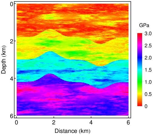
In this section, we present numerical results for CG-GMsFEM and DG-GMsFEM with two models. We consider different choices of snapshot spaces such as local-fine grid functions and harmonic functions and use different local spectral problems such as no-oversampling and oversampling described in the paper. For the first model, we consider the medium that has no-scale separation and features such as high conductivity channels and isolated inclusions. The Young’s modulus $E(x)$ is depicted in Figure 2, $\lambda(x)=\frac{\nu}{(1+\nu)(1-2\nu)}E(x)$, $\mu(x)=\frac{1}{2(1+\nu)}E(x)$, the Poisson ratio $\nu$ is taken to be $0.22$. For the second example, we use the model that is used in [11] for the simulation of subsurface elastic waves (see Figure 3). In all numerical tests, we use constant force and homogeneous Dirchlet boundary condition. In all tables below, $\Lambda_{*}$ represent the minimum discarded eigenvalue of the corresponding spectral problem. We note that the first three eigenbasis are constant and linear functions, therefore we present our numerical results starting from fourth eigenbasis in all cases.

Before presenting the numerical results, we summarize our numerical findings.

• •

  We observe a fast decay in the error as more basis functions are added in both CG-GMsFEM and DG-GMsFEM

• •

  We observe the use of multiscale partition of unity improves the accuracy of CG-GMsFEM compared to the use of piecewise bi-linear functions

• •

  We observe an improvement in the accuracy (a slight improvement in CG case and a large improvement in DG case) when using oversampling for the examples we considered and the decrease in the snapshot space dimension

In this section, we present error analysis for both no oversampling and oversampling cases. In the below, $a\preceq b$ means $a\leq Cb$, where $C$ is a contant that is independend of the mesh size and the contrast of the coefficient.

References

• [1] Assyr Abdulle. Analysis of a heterogeneous multiscale fem for problems in elasticity. Mathematical Models and Methods in Applied Sciences, 16(04):615–635, 2006.
• [2] Marco Buck, Oleg Iliev, and Heiko Andrä. Multiscale finite element coarse spaces for the application to linear elasticity. Central European Journal of Mathematics, 11(4):680–701, 2013.
• [3] Li-Qun Cao. Iterated two-scale asymptotic method and numerical algorithm for the elastic structures of composite materials. Computer methods in applied mechanics and engineering, 194(27):2899–2926, 2005.
• [4] E. Chung, Y. Efendiev, and C. S. Lee. Generalized mixed multiscale finite element method for flows in heterogeneous media. 2014. submitted.
• [5] Y. Efendiev, J. Galvis, and T. Hou. Generalized multiscale finite element methods. JCP, 251:116–135, 2013.
• [6] Y. Efendiev, J. Galvis, R. Lazarov, M. Moon, and M. Sarkis. Generalized multiscale finite element method. symmetric interior penalty coupling. Journal of Computational Physics, 255(0):1 – 15, 2013.
• [7] Y. Efendiev, J. Galvis, G. Li, and M. Presho. Generalized multiscale finite element methods. oversampling strategies. IJMM.
• [8] Y. Efendiev, R. Lazarov, M. Moon, and K. Shi. A spectral multiscale hybridizable discontinuous galerkin method for second order elliptic problems. CMAME, 2014. submitted.
• [9] Y. Efendiev, R. Lazarov, and K. Shi. A multiscale HDG method for second order elliptic equations. Part I. Polynomial and homogenization-based multiscale spaces. ArXiv e-prints, October 2013.
• [10] Gilles A Francfort and François Murat. Homogenization and optimal bounds in linear elasticity. Archive for Rational Mechanics and Analysis, 94(4):307–334, 1986.
• [11] K. Gao, S. Fu, R. Gibson, E. Chung, and Y. Efendiev. Generalized multiscale finite element method for elastic wave equations. Expanded SEG Abstracts 2014. submitted.
• [12] Xiao-Qi Liu, Li-Qun Cao, and Qi-Ding Zhu. Multiscale algorithm with high accuracy for the elastic equations in three-dimensional honeycomb structures. Journal of computational and applied mathematics, 233(4):905–921, 2009.
• [13] Olga Arsen’evna Oleinik, AS Shamaev, and GA Yosifian. Mathematical problems in elasticity and homogenization, volume 2. Elsevier, 2009.
• [14] Jörg Schröder. A numerical two-scale homogenization scheme: the fe2-method. In Plasticity and Beyond, pages 1–64. Springer, 2014.
• [15] Pham Chi Vinh and Do Xuan Tung. Homogenized equations of the linear elasticity theory in two-dimensional domains with interfaces highly oscillating between two circles. Acta mechanica, 218(3-4):333–348, 2011.