Dependent Nonparametric Bayesian Group Dictionary Learning for online reconstruction of Dynamic MR images
Abstract
In this paper, we introduce a dictionary learning based approach applied to the problem of real-time reconstruction of MR image sequences that are highly undersampled in k-space. Unlike traditional dictionary learning, our method integrates both global and patch-wise (local) sparsity information and incorporates some priori information into the reconstruction process. Moreover, we use a Dependent Hierarchical Beta-process as the prior for the group-based dictionary learning, which adaptively infers the dictionary size and the sparsity of each patch; and also ensures that similar patches are manifested in terms of similar dictionary atoms. An efficient numerical algorithm based on the alternating direction method of multipliers (ADMM) is also presented. Through extensive experimental results we show that our proposed method achieves superior reconstruction quality, compared to the other state-of-the- art DL-based methods.
I Introduction
Magnetic Resonance Imaging (MRI) is essential noninvasive tool for visualization and diagnosis of the anatomy and function of the body. It is however burdened by its intrinsic slow data acquisition process. Since data acquisition is sequential in MR imaging modalities, the scan time (time to get enough data to accurately reconstruct one frame) is reduced if fewer measurements are needed for reconstruction. The main goal of much research efforts is to be able to use a smaller set of samples than normally required to reconstruct the original images. However, when -space is under sampled, the Nyquist criterion is violated, and conventional Fourier reconstructions exhibit aliasing artifacts.
Compressed sensing (CS) [1, 2, 3, 4], on the other hand, has been shown to be able to overcome these challenges and recover MRI images from much smaller k-space measurements than conventional reconstruction methods. To achieve this, earlier CS-based methods assumed that the MRI images have a sparse representation in some known transform domain such as Wavelets [5, 6, 7, 8] Contourlet [9], finite difference domains [10].
Most of the prior work in compressed sensing MRI has been based on pre-constructed sparsifying transform. Even though pre-defined transformations are easier to implement, it was shown that such transforms sometimes lead to an insufficient and over-simplistic sparse representation of images which can usually capture only one feature of the image. For example, the widely used 2D Wavelets is able to recover point-like features but fails to capture geometric regularity such as smooth contours, Contourlets can sparsely represent curve-like features but not the points in images and finite difference may lead to staircase artifact [11]. Therefore, compressed sensing MRI (CSMRI) with nonadaptive, global sparsifying transforms, is usually limited in typical MR images to 2.5-3 fold undersampling [12].
To tackle the problems of these global transforms, some recent methods enforced the sparsity on image subregions called patches. The shift from using global image sparsity to patch-based sparsity is crucial in capturing local image features and has been shown to potentially remove noise and aliasing artifacts [13, 11]. An example of such methods is the patch-based directional wavelets method (PBDW) [13] in which authors proposed to rearrange the pixels of each patch parallel to the geometric direction of that patch and then perform the Wavelet transform. More recently, [11] proposed to use block matching to group similar patches together and then performed 3D Haar wavelet transform on each stack of similar patches. The proposed approach is shown to achieve greater sparsity than the conventional global Wavelet transform due to the similarity of the patches in each group. Although these methods avoided some of the problems associated with pre-defined representations, they still lack the ability to contain a variety of underlying features, such as edges and textures.
As an alternative, finding (learning) an adaptive patch-level basis (called dictionary), specifically tailored to the image under consideration, is shown to yield significantly enhanced performance in MR image reconstruction [14, 12, 15]. Dictionary Learning (DL) has been applied to MR images as a sparsifying basis for reconstruction (e.g., K-SVD LOST[16] and DLMRI [12]). The major problem with these methods also known as parametric DL methods, is their dependence on the initial value of patches’ sparsity level and number of dictionary atoms. When these settings do not agree with ground truth, the performance can significantly degrade. To avoid this, [17] applied a Beta-bernoulli process as a nonparametric Bayesian method for adaptive learning of dictionaries. Their work, based on Beta Process Factor Analysis (BPFA) [18], is utilized in [19] for image in-painting. [15] also applied BPFA in combination with a total variation regularization term to reconstruct MR images from undersampled space. Another method, dependent Hierarchical Beta Process (dHBP) [20], tried to improve upon BPFA results with imposing a prior belief that patches with similar features are likely to be manifested in terms of similar dictionaries. The similarity in this method is defined to be the spatial distance between the location of the patches.
The above reported works are all concerned with reconstruction of static MRI image slices and not sequences of MRI images as in volumetric (3D) or dynamic MR imaging. Currently these applications, such as real-time cardiac MRI (rtCMR) or functional MRI (fMRI), are only possible with a compromise on the achievable spatial/temporal resolution. High spatial resolution is needed for visualization of fine details or structures that have diagnostic importance. Simultaneously, the MR image sequence needs to have high temporal resolution to be able to depict changes over time due to motion or intensity variation [21, 22]. Thus, reconstruction methods specifically adapted for dealing with dynamic sequences of MRI images, can greatly benefit these applications.
However, not much has been done in the field of DL to deal with sequences of MR images. Only recently [23] and [24] extended parametric DL to dynamic MRI by jointly reconstructing the entire sequence and treating it as higher dimensional data. Through the use of patches, extracted along both the spatial and temporal directions, a single spatio-temporal 3D dictionary is trained to encode the whole dataset. Sparsity is additionally enforced on the temporal gradient domain as an additional sparsifying transform. Both of these methods fall into category of non-causal (or batch-based) methods. In non-causal approaches, the entire frames needs to be acquired before carrying out the reconstruction, which takes advantage of the temporal sparsity. The main limitation of such methods is their computational complexity and memory requirement, which for a -frame acquisition, is roughly times and times of that of causal methods, respectively. For example in DLTG method [24], the reconstruction time is reported to be about 6.6 hours for a sequence of 30 MR images. The high computational complexity of DL process is often avoided by either learning the dictionary offline form a training set or using only partial patches to train a global dictionary. Therefore, these dictionaries may fail to sparsely represent patches that are not involved in training [13].
Another limitation of such methods is that online reconstruction of images is not possible [22]. Causal approaches can recover the current frame as soon as its MR data gets acquired, and their memory and computational demand is much lower than that of non-causal (batch) methods. They are especially suitable for real-time reconstruction of MRI images. To the best of our knowledge, no DL based method has been proposed for causal reconstruction of MRI sequences.
In this paper, we propose a novel DL-based algorithm for online reconstruction of sequence of MR images from highly undersampled -space with the following features:
- •
The algorithm consists of both patch-based (local) and global sparsity terms. This is based on the observation that each of global and patch-based sparsity has its own advantages and short-comings (i.e. local image sparsity do not take into account additional image-level constraints and vise versa).
- •
To avoid the high computational complexity of the DL stage, imposed by the number of patches, and also to train more structured dictionaries, group patching is employed to classify the patches based on their similarities. The grouping is done once at the initialization step, using a guide image.
- •
A modified dHBP is utilized as the prior for the dictionary learning process. Number of dictionary elements and their relative importance is inferred non-parametrically. In addition, the model uses patch similarities and spatial closeness to encourage sharing of information within image subregions.
- •
The method is specially adopted for reconstruction of dynamic MR images. To this end, some useful prior information are extracted from the reconstructed image of the previous time instant. This priori information guides the reconstruction, through the incorporation into the global sparsity term and also through the initialization stage of the in situ DL process, in which dictionaries are learnt a priori from a fully sampled reference image(s) and then propagated and updated along the temporal dimension to include new features in the current frame.
The rest of the paper is organized as follows. This section ends with a description of the notations used. Section II presents the details of our proposed algorithm as applied to sequences of MRI images. We present and analyze our experimental results in section III before providing concluding remarks in section IV.
Notations: Throughout the paper, matrices are denoted by capital boldface letters (e.g. ), vectors are denoted by boldface small letters and we use the notation to denote the sub-matrix containing elements of with indices belonging to set . denotes the element of . Scalars are shown by regular letters (e.g. ) and linear maps are denoted by bold calligraphic uppercase letters (). Superscript added to a matrix refers to that of time .
II Dictionary learning for sequences of MR images

The problem can be posed as follows: let be the slowly time-varying MRI image of interest at epoch which is known to have an approximately sparse representation in some transform domains such as Daubechies wavelets [25, 26]. Let denote its support in Wavelet domain. It is assumed that for the first time frame a high sampled image is available (), from thereafter at each time instant, the under-sampled -space acquisition can be expressed by a linear system given as: . is the observation vector and is the measurement noise with finite energy (i.e. ), which can be modeled as a complex Gaussian noise. We define as the patch decomposition operator which extracts vectorized patches of size from the image. The vectorized patch of size is expressed as for . These patches overlap with a shift of one pixel and wrap around the image at the boundaries. Figure 1 shows some random patches of size 66 extracted from a sequence of Cardio MR images evolving with time. It is not surprising that these patches continue to be closely related to each other as they evolve over time. This property has been used extensively in other batch-based dynamic MRI reconstruction methods by enforcing the temporal gradient to be sparse [23, 24]. We also utilize this property but the key difference is that our method is causal, thus we only assume that at each time epoch , only the reconstructed image of the previous time instant (or a fully sampled reference image) is available.
Each patch of image , is assumed to be represented as a linear combination of a sparse set of atoms from a dictionary (). The goal in the simplest setting is to learn and in so doing infer by solving:
| (1) |
where enforces sparsity on .
Reformulating the above constrained optimization problem using Lagrangian multipliers we get:
| (2) |
where the weight depends on the standard deviation of the measurement noise. The first and second term in (2) represents the quality of the sparse approximations of the image patches with respect to the trained dictionary while the third one enforces data consistency in -space.
The resulting optimization is however non-convex and of combinatorial nature and thus one can only hope to reach a local minimum at best [27]. Different methods have been proposed to solve the above optimization, however they are all burdened by a heavy computational complexity of the DL process which grows rapidly with the number of patches. Reducing the number of patches is possible through either increasing each patch size () or using non-overlapping patches, however it is known that these approaches degrade the performance of DL-based methods (see Figure 10)[27]. As an alternative, we make use of the pattern redundancy in the images, which is the root of self-similarity property [11] and propose to perform patch grouping before the DL process. This is discussed in following section.
II-A Patch Grouping
The idea is that instead of using all the patches to train a single global dictionary, we classify the patches based on their similarities, so that each group only contains patches that are closely related to each other and then train different dictionaries for each group. We found that benefit of this approach is two-fold. Firstly, the number of patches is reduced for each DL process and since the learning stage is separate for each class, DL can be performed concurrently for all the classes which significantly speeds up the computation. Secondly, since the patches in each class are closely related, it is anticipated that the trained dictionaries become more structured and tailored to that specific group (see Figure 12).
To this end we aim to partition patches into groups so that each patch belongs to only one group. We also define similarity as the norm distance between patches’ intensity, where a smaller distance corresponds to more similarity. To this end, we have used k-mean [28] as a fast and efficient heuristic algorithm, to perform the grouping.
Since the -space data is undersampled, there are no available ground truth images to learn the similarity. In our proposed method, the grouping is guided based on the assumption that (or a training image) is available and that the patches are changing slowly with time, we propose to use this guide image for the grouping. As discussed in greater detail in section III, this is found to be more efficient than grouping the patches based on the zero-filled reconstructed image. Moreover, this grouping can be even done off-line before the acquisition process. If for stores the index of patches belonging to the group, (2) can be rewritten as:
| (3) |
where is the dictionary learnt for each group . Figure 2 shows an example of how patches are grouped for a Cardio image.
II-B Global sparsity and Priori knowledge
A main limitation of the DL methods that are only based on patch-level (local) sparsity is that they do not take image-level constraints such as smoothness into account. Our aim is to first add a global sparsity term to our problem formulation and secondly, to make use of any available priori-knowledge by incorporating it into the reconstruction process. To this end, we combine a global sparsity term, as the regularization of the reconstruction, by enforcing the image of interest to be sparse in the Wavelets domain. Moreover, we incorporate the priori-knowledge which is available from a reference image () to guide the reconstruction of the current image of interest (). Inspired by recent works [29, 22] that exploited the Wavelet sparsity of each frame of an image sequence with respect to a reference image, we also extend the use of such a-priori into to DL process. For the global sparsity, we use the support of the reference frame () as a close estimate to the support of the signal of interest () and then use this estimate to reconstruct by finding a signal which satisfies the observations and is sparsest outside in the Wavelets domain. This is equivalent to solving the following optimization problem:
| (4) |
where is the reference image which can either be or and . As for the incorporation of the priori-knowledge into the DL process, this is done through initialization stage of the optimization and is explained in further detail in section II-C.
II-C Optimization algorithm
To solve the optimization problem (4) we use a simple and efficient method based on the Alternating Direction Method of Multipliers (ADMM) [30, 31]. The idea is to use an additional augmented Lagrangian term to split the objective function into different conditionally independent and separable components and then solve each part sequentially until it converges. To this end a new variable () is introduced such that . Then (4) can be re-written as
| (5) |
The augmented Lagrangian form of (5) is:
| (6) |
where is the augmented Lagrangian dual variable and we add a scalar before to make things simple without affecting the results. Now, (6) can be decomposed into three separate minimization problems as:
| (7a) | ||||
| (7b) | ||||
| (7c) | ||||
| (7d) | ||||
where first in (7a) we fix and and solve for . Then using the updated value of () we learn the dictionaries from (7b). With the obtained and , we then reconstruct such that it is consistent with the space measurements by solving the minimization of (7c) over . Finally we update the dual variable . These steps are repeated until convergence (see Algorithm 2). The details of solving the above minimization problems are as follows:
Solving (7a)
Solving (7b)
To solve the non-convex objective function (7b), we use a nonparametric Bayesian-based method. Here the goal is to compute for and the corresponding sparse coefficients using a stochastic optimization method. To achieve this, a beta process is used as a prior density and consequently, the posterior density of the dictionaries and the parameters of the model is inferred using the Gibbs sampling method [33]. Let us define to be the elementwise product of a Gaussian vector () with a binary vector . Thus, for each patch belonging to group , i.e. we have
where represents the Hadamard product, , , and indicates whether for the patch , the dictionary element is active or not, is also the residual error. For each group , the dictionary size () is initially set to be large, and its actual value is inferred using Gibbs sampling.
Our goal is to incorporate two important features into our Bayesian nonparametric method: First, based on an intuition that similar patches in an image are consist of similar dictionary atoms, we want to encourage patches close to each other in one group, in terms of a defined similarity measure, to utilize similar values of . Second, based on the assumption that a reference image is available, and also that the image of each frame is closely related to the one of the previous time instant, we want to design a dynamic method such that it uses the reference image as an initialization guide, then it propagates/updates the dictionaries along the temporal direction to include new features of the current frame.
To this end, we have adopted the dependent hierarchical beta process (DHBP) [20] to find the dictionaries for each group of patches. In addition, we consider the similarity of patches in each frame and the information of first frame in the model construction. To achieve a sparse representation for the coefficients , a beta process is assigned to it in the initialization step. Moreover, the distance between the patches of each group is also considered in the initialization step.
We define a kernel that shows the similarity of two patches and takes both the spatial location and intensity values of both patches into account as:
where represents the intensity difference of two patches and is the kernel width. Note that assumes a maximum value of 1 in the case where two patches are identical and diminishes with increasing distance between the pixel values of and . It becomes 0 if two patches do not belong to a same group or if they are not located in the spatial vicinity (neighborhood) of each other. We then define a matrix such that each of its rows sums to one as:
Matrix , which manifest the interrelation of all the patches, is then used in an analogous manner to the covariates matrix in [20], to impose a priori-belief such that similar patches are more likely to employ similar dictionary settings.
It should be noted that at the initialization step of our algorithm, the kernel represents the similarity of patches for the current and first frames (reference frame) , while in the other iterations, it shows the similarity of patches with each other on the same frame .
The parameters of the model are initialized in the hierarchical framework as described in algorithm 1. For the first frame, the columns of , and is initialized with a Gaussian prior and a beta-Bernoulli process is placed as a prior for . Moreover, a gamma hyper-priors is considered for the parameters of and ( and ). For the subsequent frames, the parameters , and are initialized using the posterior density of the first frame. Moreover, is a Bernoulli process of the weighted summation of beta processes. The weight is defined using the matrix . The parameters of the DNBG method which should be learned using Markov Chain Monte Carlo (MCMC) algorithm are . The posterior density of these paprmeters is calculated in the appendix 1.

- (a)
Construct number of dictionaries as :
, for
, for - (b)
Draw a probability for each element of :
- (c)
Draw precision values for noise and each weight
, - (d)
For the patch in :
(i)Draw the vector .
(ii)Draw the binary vector with elements
(iii)Define by an element-wise product.
(iv)Construct the patch with noise. - (e)
Construct the image as the average of all patches.
Input: ,
Output:
- (a)
Initialization: dictionary variables using Algorithm1, , .
- (b)
Solving (7c)
Problem (7c) is a least squares problem with an analytical solution given as:
| (9) |
Note that term represents the reconstructed image obtained by averaging the contributions of the various patches. We observe that inverting the left matrix is computationally prohibitive. However, it is known from [32] that a simplification can be obtained by transforming from image space to Fourier space. The overview of our proposed method, called Dependent Nonparametric Bayesian Group Dictionary Learning (DNBG) is shown in Figure 2 and also Algorithm 2.
III Experimental Results
The proposed DNBG method was tested on 3 sequences of MRI images (see details in Table I11 1 Cardiac data set was provided by the Department of Diagnostic Imaging of the Hospital for Sick Children in Toronto, Canada. These images were scanned with a GE Genesis Signa MR scanner using the FIESTA scan protocol. The single slice brain perfusion MRI data set was obtained from amulti slice 2-D dynamic contrast enhanced (DCE) patient scan at the University of Rochester [34] and the thorax data set were acquired at the National University Hospital, Singapore. ) some of which are shown in Figure 3.

| Data set | Cardiac | Brain | Thorax |
|---|---|---|---|
| Bits allocated | 8 | 8 | 16 |
| Rows columns | 256 256 | 128 128 | 384 384 |
| Slices | 20 | 60 | 20 |
| Pixel size (mm) | 0.93 0.93 | – | 0.64 0.64 |
| Inter-slice spacing | 6 | – | 0.9 |
| Modality | MRI | MRI | MRA |


Sampling
Radial sampling with uniformly spaced rays in the -space domain, has been widely used for compressed MR image reconstruction [23] as it provides an incoherent measurement basis. Figure 4 shows the sampling masks used in our experiments with two different sampling ratios R, defined as . For the first image frame () in each sequence, we set R= (Figure 4(a)) since no priori knowledge is available while for the successive frames, we consider several subsampling rates (Figure 4(b)).
Parameters settings
Patches are extracted from the images in size of 44 and the dictionaries’ initial size is set to be = 128. Recall that the actual number of dictionary elements is inferred to be a smaller number. Number of groups is also set to 11 and the neighborhood (search) range is assumed to be 13. The choice of these parameters that are specific to the DNBG method is discussed in section III-B. Moreover, assuming a noiseless sampling, we set the data consistency parameter , i.e. we only allow DNBG to fill in the missing k-space. We also set , , , , = , , and . We run 100 iterations of the algorithm 2 and present the results of the last iteration.
Performance measures
To evaluate the quality of the reconstruction, we use the Peak signal-to-noise ratio (PSNR) to measure the difference of reconstructed image and the fully sampled image which is assumed to be the ground truth as:
where, is the fully sampled image and is the fully sampled image of time .
III-A Reconstruction results
We compared our algorithm with three other state-of-the art DL-based methods. (a) DLMRI method [12], which is based on K-SVD, (b) BPFA [15] which is a nonparametric bayesian dictionary learning method and (c) Blind Compressive Sensing (BCS) [34] which is the current state-of-the-art batch-based method specifically developed for the reconstruction of MR sequences 22 2 The implementation codes for DLMRI and BCS methods were obtained from http://www.ifp.illinois.edu/~yoram/DLMRI-Lab/DLMRI.html and http://research.engineering.uiowa.edu/cbig/content/software.


Figure 5 shows the reconstruction performance of our proposed method, compared against other methods, in terms of the PSNR value at different k-space sample rates. For each sample rate the mean and standard deviation of reconstructed result of all frames has been shown. It can be seen that for all data sets, DNBG out-performs other methods, in terms of both higher mean performance and smaller standard deviation of the reconstruction results. This is more profound for the cardiac data set. Although BPFA and DNBG both utilize nonparametric bayesian model for the DL, the PSNR of DNBG is significantly higher due to the grouping and incorporation the dependency of patches. It is also observed that in some settings BCS tends to achieve comparable mean PSNR performance to our method. However, its std is consistently much higher than our method i.e. its performance maybe quite different from one frame to another.
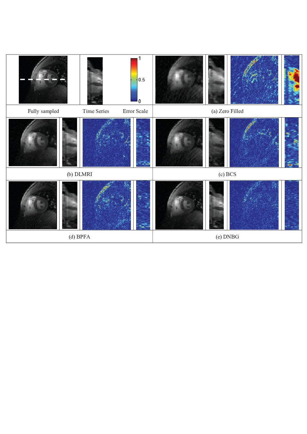
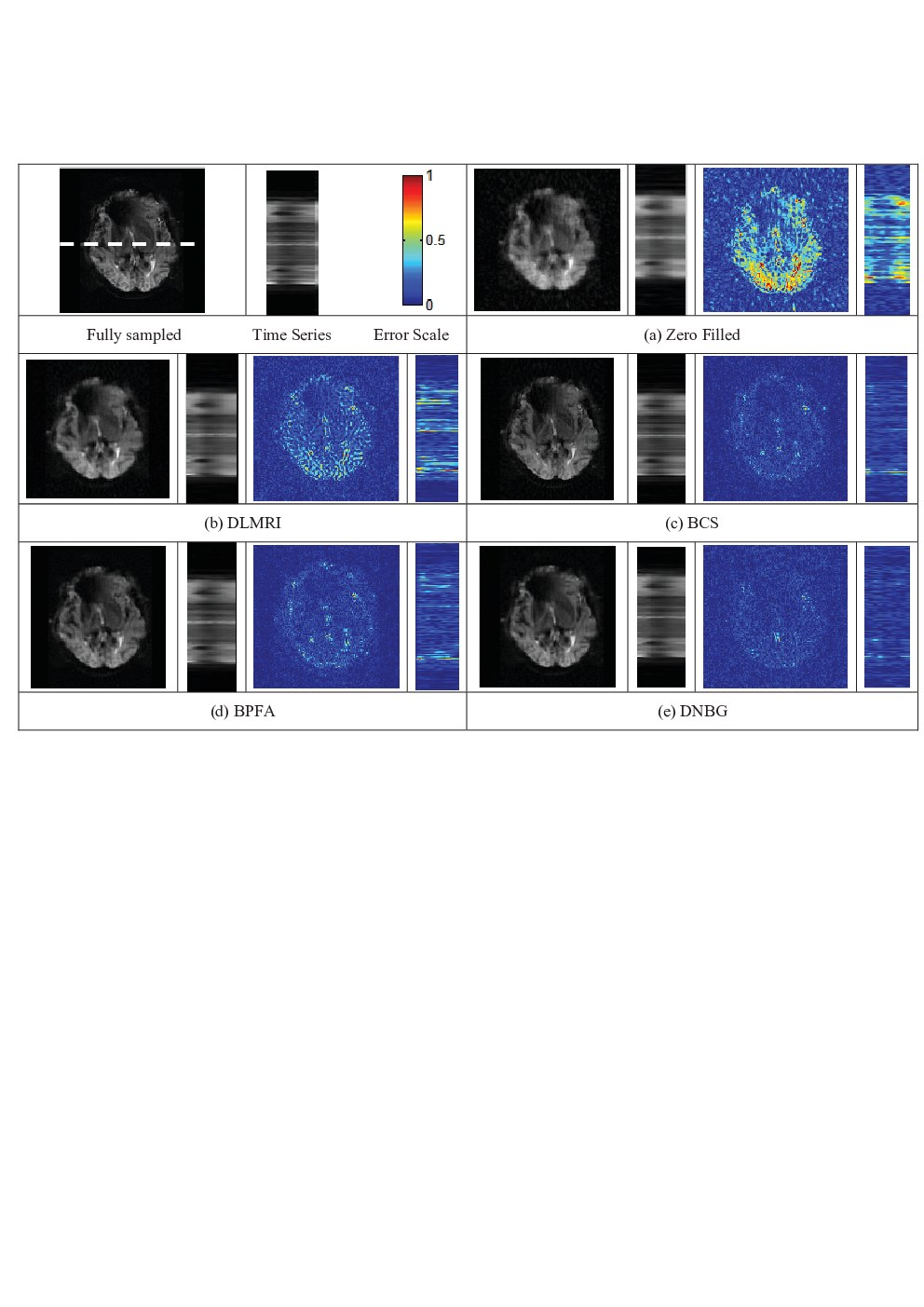
To also compare the visual quality of the reconstructed images, Figures 6-7 show the reconstruction result of our method against others for the cardiac, brain and thorax data sets, respectively. The original frame, together with the original image time profile through the dotted line is shown in the top left cell. For each method the reconstruction image and time profile, together with the error amplified by a factor of 4 is also shown. Note that for the cardiac and thorax data set, what is shown is a ROI in which we have highest variation in time. From these figures, it is evident that our method achieved superior visual reconstruction quality. It is specially noted that the reconstruction error of other methods is mainly concentrated near the boundaries that are changing.

III-B Discussion about the choise of parameters
The performance of the proposed method depends on the number of patch groups (), patch size () and neighborhood range (). We now discuss the behavior of our method with respect to changes in these parameters.
Dependence on
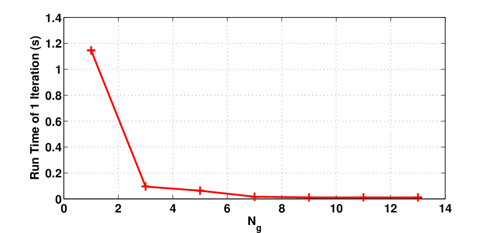
Figure 9(a), shows the run-time of one iteration of our algorithm vs. the number of groups (). From the figure it can be seen that grouping the patches even into 2 groups can significantly speed-up the computations. It is observed that up to the computation complexity of the DL process is inversely proportional to the number of groups and thereafter it is almost constant. On the other hand, Figure 9(b) shows the mean and variance of the reconstruction error as a function of . It can be seen that the performance improves as increases and is the highest possible for a range of up to beyond which the error begins to increase. This observation is inline with Figure 9(c), which shows the sparsity of , measured using the Gini Index (GI) [35], as a function of . It can be seen that increasing group number also increases the sparsity of (since the GI is closest to 1), which means that smaller number of dictionary atoms are needed to represent a patch. This could be due to the reason that the trained dictionaries are more tailored to that specific group and are better able to represent a patch belonging to that class. On the other hand, increasing beyond 12 decreases ’s sparsity significantly.


Dependence on patch size
Figure 10 shows the sensitivity of our proposed method, to the chosen patch size, in terms of the reconstruction error. It can be seen from the figure that increasing the patch size, beyond 6 deteriorates the performance. This is expected since local information is not well captured when the patches are too large. On the other hand, smaller patch size results in an increased number of patches and consequently higher computational complexity. We found to be a good trade-off between the computational complexity and the algorithm’s performance.

Dependence on
Figure 11 shows the reconstruction error as a function of the defined neighborhood range (). It can be seen that our method is not sensitive to the search range and the reconstruction error only slightly decrease with the increase of . Considering that widening the search range calls for higher computational effort and also that not much reconstruction gain is achieved, we set to be 13.


III-C Summary and Future work
Through several experiments we demonstrated the superiority of the proposed DNBG method in terms of both quantitative and qualitative reconstruction results and also the reduced computational complexity which is due to the grouping of the patches. Patch grouping results in significantly smaller number of patches to be handled for each class. Moreover, since the patches in each class are closely related, trained dictionaries (see Figure 12) are more tailored to that specific group. This is also evident from sparsity of , which indicates that a smaller number of dictionary atoms are needed to represent a patch. In addition, in contrast to BCS that only exploits the temporal correlations, our method uses both the spatial and temporal correlations adaptively through the learned dictionaries.
While our proposed method is developed for the single-coil MRI modality, it is possible to incorporate ”parallel imaging” [36] into the proposed method by changing the -space encoding matrix to a sensitivity encoding one. It should be noted that acquiring accurate coil sensitivities for time frame can be challenging [37]. This will be investigated in our future study.
IV Conclusion
In this paper, we presented a dictionary learning based approach which enables a detailed and fast reconstruction of the dynamic MRI images from highly undersampled k-space. Our proposed method has three major improvements over the state-of-the-art dictionary-based method. Firstly, it combines both the global and patch-based sparsity. Secondly it uses patch grouping for the DL process to reduce computational complexity and also to train dictionaries that are more structured. Lastly, it uses temporal and spatial correlation of the patches and encourages close ones to employ similar dictionary settings. Through extensive experiments, our proposed method has been shown to consistently achieve superior reconstruction quality, in terms of PSNR and visual quality, with much less computational complexity than the state-of-the-art methods.
V Appendix
The parameters of the DNBG method, , are learned using Markov Chain Monte Carlo (MCMC) algorithm. We adopted the Gibbs sampling update equations stated in [15] and [20] and extended them for the DNBG model as follows:
| (10) | ||||
where and and is the column of the .cite
| (11) | ||||
| (12) |
where is the error of computing the ith patch with all dictionaries of DNBG except kth dictionary element,
| (13) |
| (14) | ||||
| (15) |
References
- [1] E.J. Candes and T. Tao, “Near-optimal signal recovery from random projections: universal encoding strategies?,” IEEE Trans. on Information Theory, vol. 52, no. 12, pp. 5406 – 25, 2006.
- [2] E.J. Candes, J. Romberg, and T. Tao, “Robust uncertainty principles: exact signal reconstruction from highly incomplete frequency information,” IEEE Trans. on Information Theory, vol. 52, no. 2, pp. 489 – 509, 2006.
- [3] E.J. Candes and M.B. Wakin, “An introduction to Compressive Sampling,” IEEE Signal Processing Magazine, vol. 25, no. 2, pp. 21 – 30, 2008.
- [4] David Donoho, “Compressed Sensing,” IEEE Trans. on Information Theory, vol. 52, no. 4, pp. 1289 – 1306, 2006.
- [5] Michael Lustig, David Donoho, and John M. Pauly, “Sparse MRI: The application of Compressed Sensing for rapid MR imaging,” Magnetic Resonance in Medicine, vol. 58, no. 6, pp. 1182–1195, 2007.
- [6] J.P. Haldar, D. Hernando, and Zhi pei Liang, “Compressed-sensing MRI with random encoding,” Medical Imaging, IEEE Transactions on, vol. 30, no. 4, pp. 893–903, April 2011.
- [7] Angshul Majumdar and Rabab K Ward, “An algorithm for sparse MRI reconstruction by schatten -norm minimization,” Magnetic resonance imaging, vol. 29, no. 3, pp. 408–417, 2011.
- [8] Ashraf A. Kassim, Yan Niu, and Dornoosh Zonoobi, “Wavelet packet transform basis selection method for set partitioning in hierarchical trees.,” Electronic Imaging, vol. 17, no. 3, pp. 033007, 2008.
- [9] S.M. Gho, Y. Nam, E.Y. Kim S.Y. Zho, and D.H. Kim, “Three dimension double inversion recovery gray matter imaging using Compressed Sensing,” Magnetic Resonance Imaging, vol. 28, no. 10, pp. 1395–1402, 2010.
- [10] J. D.Trzasko, C.R. Haider, N.G. Campeau E.A. Borisch, J.F. Glockner, S.J. Riederer, and A. Manduca, “Sparse-CAPR: Highly accelerated 4D CE-MRA with parallel imaging and nonconvex compressive sensing,” Magnetic Resonance Imaging, vol. 66, pp. 1019–1032, 2011.
- [11] Xiaobo Qu, Yingkun Hou, Fan Lam, Di Guo, Jianhui Zhong, and Zhong Chen, “Magnetic Resonance image reconstruction from undersampled measurements using a patch-based nonlocal operator,” Medical image analysis, in press, 2013.
- [12] Saiprasad Ravishankar and Yoram Bresler, “MR image reconstruction from highly undersampled k-space data by dictionary learning,” IEEE Transactions on Medical Imaging, vol. 30, no. 5, pp. 1028–1041, 2011.
- [13] Xiaobo Qu, Di Guo, Bende Ning, Yingkun Hou, Yulan Lin, Shuhui Cai, and Zhong Chen, “Undersampled MRI reconstruction with patch-based directional wavelets,” Magnetic resonance imaging, vol. 30, no. 7, pp. 964–977, 2012.
- [14] M. Aharon, M. Elad, and A. Bruckstein, “ -SVD: An algorithm for designing overcomplete dictionaries for sparse representation,” Signal Processing, IEEE Transactions on, vol. 54, no. 11, pp. 4311–4322, Nov 2006.
- [15] Y. Huang, J. Paisley, Q. Lin, X. Ding, X. Fu, and X.-p. Zhang, “Bayesian nonparametric dictionary learning for compressed sensing mri,” Image Processing, IEEE Transactions on, vol. 23, no. 12, pp. 5007–5019, 2014.
- [16] Mehmet Akçakaya, Tamer A Basha, Beth Goddu, Lois A Goepfert, Kraig V Kissinger, Vahid Tarokh, Warren J Manning, and Reza Nezafat, “Low-dimensional-structure self-learning and thresholding: Regularization beyond Compressed Sensing for MRI reconstruction,” Magnetic Resonance in Medicine, vol. 66, no. 3, pp. 756–767, 2011.
- [17] Qin Lin, Wei Guo, Xueyang Fu, Xinghao Ding, and Yue Huang, “MR image reconstruction by patch-based sparse representation,” Journal of Theoretical and Applied Information Technology, vol. 49, no. 1, pp. 107–112, 2013.
- [18] John Paisley and Lawrence Carin, “Nonparametric factor analysis with beta process priors,” in Proceedings of the 26th Annual International Conference on Machine Learning. ACM, 2009, pp. 777–784.
- [19] Mingyuan Zhou, Haojun Chen, John Paisley, Lu Ren, Lingbo Li, Zhengming Xing, David Dunson, Guillermo Sapiro, and Lawrence Carin, “Nonparametric bayesian dictionary learning for analysis of noisy and incomplete images,” Image Processing, IEEE Transactions on, vol. 21, no. 1, pp. 130–144, 2012.
- [20] Mingyuan Zhou, Hongxia Yang, Guillermo Sapiro, David B Dunson, and Lawrence Carin, “Dependent hierarchical beta process for image interpolation and denoising,” in International conference on artificial intelligence and statistics, 2011, pp. 883–891.
- [21] H. Jung, K. Sung, K. S. Nayak, E. Y. Kim, and J. C. Ye, “k-t FOCUSS: A general Compressed Sensing framework for high resolution dynamic MRI,” Magnetic Resonance in Medicine, vol. 61, no. 1, pp. 103–116, 2009.
- [22] D. Zonoobi and Ashraf A Kassim, “A computationally efficient method for reconstructing sequences of MR images from undersampled -space data,” Medical image analysis, vol. 18, no. 6, pp. 857–865, 2014.
- [23] Yanhua Wang and L. Ying, “Compressed Sensing dynamic cardiac Cine MRI using learned spatiotemporal dictionary,” Biomedical Engineering, IEEE Transactions on, vol. 61, no. 4, pp. 1109–1120, April 2014.
- [24] Jose Caballero, Anthony N Price, Daniel Rueckert, and J Hajnal, “Dictionary learning and time sparsity for dynamic MR data reconstruction,” IEEE Transactions on Medical Imaging, vol. 33, no. 4, pp. 979–994, 2014.
- [25] Dornoosh Zonoobi and Ashraf A Kassim, “Weighted-CS for reconstruction of highly under-sampled dynamic MRI sequences,” in Signal & Information Processing Association Annual Summit and Conference (APSIPA ASC), 2012 Asia-Pacific. IEEE, 2012, pp. 1–5.
- [26] D. Zonoobi and Ashraf A. Kassim, “On the reconstruction of sequences of sparse signals - The Weighted-CS,” Journal of Visual Communication and Image Representation, vol. 24, no. 2, pp. 196–202, Feb. 2013.
- [27] R. Rubinstein, A.M. Bruckstein, and M. Elad, “Dictionaries for sparse representation modeling,” Proceedings of the IEEE, vol. 98, no. 6, pp. 1045–1057, June 2010.
- [28] Amir Ahmad and Lipika Dey, “A -mean clustering algorithm for mixed numeric and categorical data,” Data & Knowledge Engineering, vol. 63, no. 2, pp. 503–527, 2007.
- [29] L. Wei, T. Li, I.C. Atkinson, and N. Vaswani, “Modified-CS-residual for recursive reconstruction of highly undersampled functional MRI sequences,” in Image Processing (ICIP), 2011 18th IEEE International Conference on, 2011, pp. 2689–2692.
- [30] Stephen Boyd, Neal Parikh, Eric Chu, Borja Peleato, and Jonathan Eckstein, “Distributed optimization and statistical learning via the alternating direction method of multipliers,” Foundations and Trends in Machine Learning, vol. 3, no. 1, pp. 1–122, 2011.
- [31] Xinghao Ding, J. Paisley, Yue Huang, Xianbo Chen, Feng Huang, and Xiao-Ping Zhang, “Compressed Sensing MRI with bayesian dictionary learning,” in Image Processing (ICIP), 2013 20th IEEE International Conference on, Sept 2013, pp. 2319–2323.
- [32] Tom Goldstein and Stanley Osher, “The Split Bregman method for -regularized problems,” SIAM J. Imaging Sciences, vol. 2, no. 2, pp. 323–343, 2009.
- [33] P. Damlen, J. Wakefield, and S. Walker, “Gibbs sampling for Bayesian non-conjugate and hierarchical models by using auxiliary variables,” Journal of the Royal Statistical Society: Series B (Statistical Methodology), vol. 61, no. 2, pp. 331–344, 1999.
- [34] Sajan Goud Lingala and Mathews Jacob, “Blind compressive sensing dynamic MRI,” IEEE Transactions on Medical Imaging, vol. 32, no. 6, pp. 1132–1145, 2013.
- [35] D. Zonoobi, Ashraf A. Kassim, and Y. Venkatesh Venkatesh, “Gini index as sparsity measure for signal reconstruction from compressive samples,” IEEE Journal of Selected Topics in Signal Processing, vol. 5, no. 5, pp. 927 –932, sept. 2011.
- [36] Xiaojing Ye, Yunmei Chen, Wei Lin, and Feng Huang, “Fast mr image reconstruction for partially parallel imaging with arbitrary-space trajectories,” Medical Imaging, IEEE Transactions on, vol. 30, no. 3, pp. 575–585, 2011.
- [37] Jose Caballero, Daniel Rueckert, and JosephV. Hajnal, “Dictionary learning and time sparsity in dynamic MRI,” in Medical Image Computing and Computer-Assisted Intervention (MICCAI ), vol. 7510 of Lecture Notes in Computer Science, pp. 256–263. 2012.