We consider the SM and quantized general relativity, in which the graviton couples with the SM particles. The gravitational coupling constant is given by $\kappa^{2}=16\pi G=16\pi/M_{\rm Pl}^{2}$, in which $G$ is the Newton constant, and the Planck mass is $M_{\rm Pl}=G^{-1/2}\simeq 1.22\times 10^{19}$ GeV. This coupling is small enough to neglect far below the Planck scale, while it is effective around the Planck scale. To see energy dependences of couplings, we have to solve the corresponding RGEs. The RGE for a coupling constant $x$ is given by

where $\beta_{x}^{\rm SM}$ and $\beta_{x}^{\rm gravity}$ are the Callan-Symanzik $\beta$ function in the SM and a gravitational contribution to the $\beta$ functions, respectively.²² 2 $\beta$ functions in the SM at the two-loop level are given in the Appendix. In our numerical analysis, we utilize the SM $\beta$ functions at the two-loop level and include the leading contributions from gravity given in Eq. (3). The gravitational contribution at the one-loop level is written by

where $a_{x}$ is a constant that denotes the gravitational contribution to the coupling $x$, and it can be obtained by calculating the corresponding graviton one-loop diagrams.

In this paper, we assume $a_{g_{1}}=a_{g_{2}}=a_{g_{3}}\equiv a_{g}$ for the SM gauge couplings as taken in [5]. This assumption seems to be valid due to the universality of the gravitational interactions. If $a_{g}$ is negative, all gauge couplings approach zero near the Planck scale. Thus, the gauge interactions are asymptotically free. In addition, the Landau pole problem for the $U(1)_{Y}$ gauge coupling in the SM can be solved due to the presence of the fixed point. References [21]-[24] obtained negative values of $a_{g}$ with $|a_{g}|\sim{\cal O}(1)$. For the top Yukawa coupling $y_{t}$, the Yukawa interaction also becomes asymptotically free when $a_{y_{t}}<0$. Regarding the Higgs quartic coupling $\lambda$, the gravitational contribution $\beta_{\lambda}^{\rm gravity}$ can be dominant around the Planck scale. Thus, the vacuum stability ($\lambda>0$ up to the Planck scale) can be more easily realized compared to the SM by taking the gravitational contribution with $a_{\lambda}>0$ into account. In fact, $a_{\lambda}=6$ was utilized in Refs. [24, 25]. We note that Refs. [26, 27] and [28] showed that the values of $a_{g}$ and $a_{y_{t}}$ depend on the gauge fixing, respectively. In addition, Ref. [29] showed that gravitational effects of the gravitational constant depend on physical processes. Therefore, we treat $a_{g}$, $a_{y_{t}}$ and $a_{\lambda}$ as free parameters in this work.

Next, we show typical gravitational effects on the RGE evolution of coupling constants. To solve the RGEs, the following BCs [12, 13] are taken,

where $M_{t}$ and $M_{h}$ are the pole masses of the top quark and the Higgs boson, respectively. The BCs of the gauge and top Yukawa couplings are determined by Eqs. (4)-(7) for given $M_{t}$ and $\alpha_{s}$. After solving the RGEs, Eq. (8) gives $M_{h}$ as

In Fig. 1, we show an example of the RGE evolution of the SM couplings that include gravitational effects, in which the above BCs are taken.

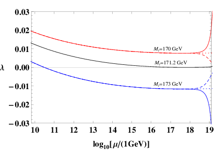
Figure 1 (a) shows typical RGE evolution of the SM couplings. The solid (dashed) lines show the RGE evolution with (without) the gravitational contributions. In the figure, we take $a_{g}=a_{y_{t}}=-1$ [5, 23], $a_{\lambda}=6$ [24, 25], $M_{t}=171.2$ GeV, $M_{h}=125.7$ GeV, and $\alpha_{s}=0.1184$, which realize $\lambda(M_{\rm Pl})=0$. The RGE evolution of gauge and top Yukawa couplings indicates asymptotic freedom of the interactions due to the gravitational contributions as mentioned above. If we take $a_{g}>0$ and $a_{y_{t}}>0$, the gauge and top Yukawa couplings become large around the Planck scale. One can see that the gravitational contributions become effective above $\mu\approx 10^{18}$ GeV. In this work, we concentrate on the energy region up to $\mu=M_{\rm Pl}$ as a physical scale, which is depicted by the vertical solid line. On the other hand, Ref. [24] mentioned that the analyses can be valid in the region of $|x^{-1}\beta_{x}^{\rm gravity}|<1$, which reads $\mu<(\pi/|a_{x}|)M_{\rm Pl}$. In this case, an effective energy region for the model is larger than the Planck scale when $|a_{x}|<\pi$. As a result, the gravitational effects with $a_{g}=-1$ may assist the gauge coupling unification since all gauge couplings unify at an energy scale lower than $\mu<\pi M_{\rm Pl}$.

Figure 1 (b) shows the $a_{\lambda}$ and $M_{t}$ dependence of the evolution of $\lambda$. We take $a_{g}=a_{y_{t}}=-1$, $M_{h}=125.7$ GeV, and $\alpha_{s}=0.1184$ in the figure. The solid, dashed, and dotted lines correspond to $a_{\lambda}=6$, $a_{\lambda}=-6$, and $a_{\lambda}=0$, respectively. The red, black, and blue lines are the cases of $M_{t}=170$ GeV, 171.2 GeV, and 173 GeV, respectively. Note that the sign of $\lambda$ in the Planck scale strongly depends on the top pole mass, e.g. $\lambda(M_{\rm Pl})\gtrless 0$ for $M_{t}\lessgtr 171.2$ GeV when we take $M_{h}=125.7$ GeV and $\alpha_{s}=0.1184$. One can understand the behaviors of $\lambda$ around the Planck scale by considering $\beta_{\lambda}$ as follows. Now $\beta_{\lambda}$ can be approximately written as

around the Planck scale. When both $a_{g}$ and $a_{y_{t}}$ are negative, the gauge and top Yukawa couplings approach zero as $\mu$ becomes large. Then, the last term (the gravitational contribution term) of Eq. (11) dominates $\beta_{\lambda}$ when $a_{\lambda}$ is sufficiently large. Thus, $\lambda$ is approximately given by

where $\mu_{*}$ is an energy scale at which the gravitational contribution becomes dominant, and $\lambda_{*}$ is a value of $\lambda$ at $\mu=\mu_{*}$. As a result, $|\lambda|$ is larger (lower) for $a_{\lambda}>0$ ($a_{\lambda}<0$) while keeping the sign of $\lambda$.

One can also see that the gravitational effects and the value of $a_{\lambda}$ slightly change the RGE evolutions of the SM couplings around the Planck scale, while they significantly change the $\beta$ functions. It should be remarked that $\beta_{\lambda}(M_{\rm Pl})=0$ can be induced from $\lambda(M_{\rm Pl})\simeq 0$ when the gravitational contributions are taken into account in the SM as seen in Eq. (11). Thus, two independent BCs of $\lambda(M_{\rm Pl})=0$ and $\beta_{\lambda}(M_{\rm Pl})=0$ predict almost the same value of the Higgs mass for a given $M_{t}$. In the next section, we quantitatively clarify regions of model parameters for the realization of the MPCP in this scenario.

We show the results of numerical analyses satisfying the NC-MPCP in Figs. 2 and 3. Figure 2 shows predictions for the Higgs and the top pole masses from the realizations of $\lambda(M_{\rm Pl})=0$ and $\beta_{\lambda}(M_{\rm Pl})=0$. In the figure, we take $a_{g}=a_{y_{t}}=-1$ and $a_{\lambda}=6$. To realize $M_{h}=125.7\pm 0.4$ GeV, the top pole mass should be in the region of $170.8~{\rm GeV}\lesssim M_{t}\lesssim 171.7~{\rm GeV}$.³³ 3 On the other hand, the experimentally favored value of the top quark mass is $173.34\pm 0.76$ GeV [30]. In Ref. [13], the authors suggest this discrepancy might not be problematic, and just the discrepancy between the pole mass and the mass obtained at the collider experiments [30]. Our predicted value is a pole of a colored quark, while the experimentally obtained value is an invariant mass of the color singlet final states. Since the observed $t\bar{t}$ pair is dominantly color octet at the hadron collider, the discrepancy of a few GeV from the singlet final states may be caused [31, 32]. The result is consistent with the previous result including gravitational effects [5].

We also show the parameter dependence of the realizations of $\lambda(M_{\rm Pl})=0$ and $\beta_{\lambda}(M_{\rm Pl})=0$ for a typical top mass as 171.2 GeV in Fig. 3. As mentioned above, $M_{t}=171.2$ GeV cannot realize the MPCP although the NC-MPCP is satisfied. The red circles and blue crosses in Fig. 3 indicate the necessary conditions of the MPCP, $\lambda(M_{\rm Pl})=0$ and $\beta_{\lambda}(M_{\rm Pl})=0$, respectively. Hence, the NC-MPCP can be satisfied at the overlapped points of red circles and blue crosses in the figure.

Let us mention the results of parameter dependence for the NC-MPCP. First, the NC-MPCP can be satisfied in almost all regions of $a_{g}<0$ and $a_{y_{t}}<0$ [see Figs. 3 (a) and 3 (b)]. Since gauge and top Yukawa couplings can be asymptotically free in this regime, $\beta_{\lambda}$ is dominated by the gravitational contribution. As a result, $\beta_{\lambda}(M_{\rm Pl})=0$ is induced from $\lambda(M_{\rm Pl})\simeq 0$ as mentioned above.

Second, regarding the value of $a_{\lambda}$ for the NC-MPCP, sufficiently large value of $|a_{\lambda}|$ such as $|a_{\lambda}|\gtrsim 2$ is typically required [see Figs. 3 (a) and 3 (b)]. When $|a_{\lambda}|$ is sufficiently large, the gravitational term is dominant in $\beta_{\lambda}$. Thus, the conditions $\lambda(M_{\rm Pl})=0$ and $\beta_{\lambda}(M_{\rm Pl})=0$ are satisfied at the same time. Note that $\beta_{\lambda}(M_{\rm Pl})=0$ cannot be realized for $-0.001\lesssim a_{\lambda}\lesssim 0.04$.

Third, when $a_{g}$ is positive, gauge couplings become larger as $\mu$ becomes large. Since the terms positively contribute to $\beta_{\lambda}$, the condition $\beta_{\lambda}(M_{\rm Pl})=0$ leads $\lambda(M_{\rm Pl})<0$. Similarly, top Yukawa coupling becomes larger for $a_{y_{t}}>0$, and the terms negatively contribute to $\beta_{\lambda}$. Then, the condition $\beta_{\lambda}(M_{\rm Pl})=0$ leads $\lambda(M_{\rm Pl})>0$. As a result, for $a_{g}>0$ ($a_{y_{t}}>0$) the NC-MPCP cannot be satisfied in most cases. However, the NC-MPCP can be satisfied when both $a_{g}$ and $a_{y_{t}}$ are positive, because the contributions of gauge and top Yukawa couplings cancel each other [see upper right region in the first quadrant of Fig. 3 (c)].

Finally, there are also regions satisfying the NC-MPCP, in which $a_{g}\gtrless 0$ and $a_{y_{t}}\lessgtr$ [e.g., see the second and fourth quadrants of Fig. 3 (c)], when both $|a_{g}|$ and $|a_{y_{t}}|$ are relatively small with sufficiently large $|a_{\lambda}|$. Since the last term of Eq. (11) can still dominate the other terms also in the regions, $\beta_{\lambda}(M_{\rm Pl})=0$ can be induced from $\lambda(M_{\rm Pl})\simeq 0$.

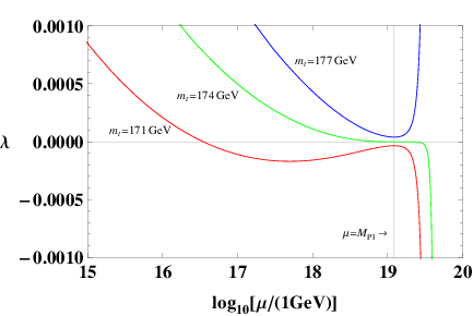
In the previous subsection, we investigate the regions of the model parameters satisfying the NC-MPCP. Figure 4 shows examples of the RGE evolution of $\lambda$ satisfying $\beta_{\lambda}(M_{\rm Pl})=0$. We take $a_{g}=a_{y_{t}}=-1$, $M_{h}=125.7$ GeV, and $\alpha_{s}=0.1184$ in the figure. The red, green and blue lines correspond to $M_{t}=171$ GeV, 174 GeV and 177 GeV, respectively. The behavior around the Planck scale is understood by Eq. (12), that is, $|\lambda|$ is larger for $a_{\lambda}>0$ as keeping the sign of $\lambda$. This figure implies that the Higgs potential has a local maximum at the Planck scale for $M_{t}\lesssim 174$ GeV, and thus the MPCP cannot be realized for $M_{t}\lesssim 174$ GeV. We find that $M_{h}\gtrsim 131.5$ GeV with $M_{t}\gtrsim 174$ GeV is required by the realization of the MPCP. Since the gravitational contribution is effective for $\mu\gtrsim 10^{18}$ GeV, these values of the Higgs and the top masses for the MPCP in our scenario are not drastically changed from the ones predicted by the past research without taking into account gravity [4] (see also [3, 6]). Therefore, we conclude that the MPCP cannot be realized in the SM and also the SM with gravity since $M_{h}\gtrsim 131.5$ GeV is experimentally ruled out.

This work is partially supported by the Scientific Grant by Ministry of Education and Science, No. 24540272. The works of R.T. and Y.Y. are supported by Research Fellowships of the Japan Society for the Promotion of Science for Young Scientists [Grants No. 24$\cdot$801 (R.T.) and No. 26$\cdot$2428 (Y.Y.)].

References

- [1] G. Aad et al. [ATLAS Collaboration], Phys. Lett. B 716, 1 (2012) [arXiv:1207.7214 [hep-ex]].
- [2] S. Chatrchyan et al. [CMS Collaboration], Phys. Lett. B 716, 30 (2012) [arXiv:1207.7235 [hep-ex]].
- [3] P. P. Giardino, K. Kannike, I. Masina, M. Raidal and A. Strumia, JHEP 1405, 046 (2014) [arXiv:1303.3570 [hep-ph]].
- [4] C. D. Froggatt and H. B. Nielsen, Phys. Lett. B 368, 96 (1996) [hep-ph/9511371].
- [5] M. Shaposhnikov and C. Wetterich, Phys. Lett. B 683, 196 (2010) [arXiv:0912.0208 [hep-th]].
- [6] M. Holthausen, K. S. Lim and M. Lindner, JHEP 1202, 037 (2012) [arXiv:1112.2415 [hep-ph]].
- [7] F. Bezrukov, M. Y. .Kalmykov, B. A. Kniehl and M. Shaposhnikov, JHEP 1210, 140 (2012) [arXiv:1205.2893 [hep-ph]].
- [8] G. Degrassi, S. Di Vita, J. Elias-Miro, J. R. Espinosa, G. F. Giudice, G. Isidori and A. Strumia, JHEP 1208, 098 (2012) [arXiv:1205.6497 [hep-ph]].
- [9] S. Alekhin, A. Djouadi and S. Moch, Phys. Lett. B 716, 214 (2012) [arXiv:1207.0980 [hep-ph]].
- [10] I. Masina, Phys. Rev. D 87, no. 5, 053001 (2013) [arXiv:1209.0393 [hep-ph]].
- [11] Y. Hamada, H. Kawai and K. -y. Oda, Phys. Rev. D 87, no. 5, 053009 (2013) [arXiv:1210.2538 [hep-ph]].
- [12] D. Buttazzo, G. Degrassi, P. P. Giardino, G. F. Giudice, F. Sala, A. Salvio and A. Strumia, JHEP 1312, 089 (2013) [arXiv:1307.3536].
- [13] Y. Hamada, H. Kawai and K. -y. Oda, arXiv:1404.6141 [hep-ph].
- [14] N. Haba, K. Kaneta and R. Takahashi, JHEP 1404, 029 (2014) [arXiv:1312.2089 [hep-ph]].
- [15] N. Haba, H. Ishida, K. Kaneta and R. Takahashi, arXiv:1406.0158 [hep-ph].
- [16] A. Spencer-Smith, arXiv:1405.1975 [hep-ph].
- [17] Z. Z. Xianyu and H. J. He, arXiv:1407.6993 [astro-ph.CO].
- [18] V. Branchina and E. Messina, Phys. Rev. Lett. 111, 241801 (2013) [arXiv:1307.5193 [hep-ph]].
- [19] J. F. Donoghue, Phys. Rev. Lett. 72, 2996 (1994) [gr-qc/9310024].
- [20] J. F. Donoghue, Phys. Rev. D 50, 3874 (1994) [gr-qc/9405057].
- [21] S. P. Robinson and F. Wilczek, Phys. Rev. Lett. 96, 231601 (2006) [hep-th/0509050].
- [22] D. Ebert, J. Plefka and A. Rodigast, Phys. Lett. B 660, 579 (2008) [arXiv:0710.1002 [hep-th]].
- [23] Y. Tang and Y. -L. Wu, Commun. Theor. Phys. 54, 1040 (2010) [arXiv:0807.0331 [hep-ph]].
- [24] H. -J. He, X. -F. Wang and Z. -Z. Xianyu, Phys. Rev. D 83, 125014 (2011) [arXiv:1008.1839 [hep-th]].
- [25] F. Wang, Nucl. Phys. B 884, 193 (2014) [arXiv:1312.1925 [hep-ph]].
- [26] A. R. Pietrykowski, Phys. Rev. Lett. 98, 061801 (2007) [hep-th/0606208].
- [27] D. J. Toms, Phys. Rev. D 84, 084016 (2011).
- [28] O. Zanusso, L. Zambelli, G. P. Vacca and R. Percacci, Phys. Lett. B 689, 90 (2010) [arXiv:0904.0938 [hep-th]].
- [29] M. M. Anber and J. F. Donoghue, Phys. Rev. D 85, 104016 (2012) [arXiv:1111.2875 [hep-th]].
- [30] [ATLAS and CDF and CMS and D0 Collaborations], arXiv:1403.4427 [hep-ex].
- [31] T. Horiguchi, A. Ishikawa, T. Suehara, K. Fujii, Y. Sumino, Y. Kiyo and H. Yamamoto, arXiv:1310.0563 [hep-ex].
- [32] M. C. Smith and S. S. Willenbrock, Phys. Rev. Lett. 79 (1997) 3825 [hep-ph/9612329].
- [33] F. L. Bezrukov and M. Shaposhnikov, Phys. Lett. B 659, 703 (2008) [arXiv:0710.3755 [hep-th]].
- [34] F. Bezrukov and M. Shaposhnikov, JHEP 0907, 089 (2009) [arXiv:0904.1537 [hep-ph]].
- [35] F. Bezrukov, A. Magnin, M. Shaposhnikov and S. Sibiryakov, JHEP 1101, 016 (2011) [arXiv:1008.5157 [hep-ph]].
- [36] N. Haba and R. Takahashi, Phys. Rev. D 89, 115009 (2014) [arXiv:1404.4737 [hep-ph]].
- [37] N. Haba, H. Ishida and R. Takahashi, arXiv:1405.5738 [hep-ph].
- [38] V. Branchina, E. Messina and A. Platania, arXiv:1407.4112 [hep-ph].