The Milky Way Tomography with SDSS. V. Mapping the Dark Matter Halo
Abstract
We present robust constraints from the Sloan Digital Sky Survey (SDSS) on the shape and distribution of the dark matter halo within the Milky Way (MW). Using the number density distribution and kinematics of SDSS halo stars, we probe the dark matter distribution to heliocentric distances exceeding 10 kpc and galactocentric distances exceeding 20 kpc. Our analysis utilizes Jeans equations to generate two-dimensional acceleration maps throughout the volume; this approach is thoroughly tested on a cosmologically derived –body+SPH simulation of a MW-like galaxy. We show that the known accelerations (gradients of the gravitational potential) can be successfully recovered in such a realistic system. Leveraging the baryonic gravitational potential derived by Bovy & Rix (2013), we show that the gravitational potential implied by the SDSS observations cannot be explained, assuming Newtonian gravity, by visible matter alone: the gravitational force experienced by stars at galactocentric distances of 20 kpc is as much as three times stronger than what can be attributed to purely visible matter. We also show that the SDSS data provide a strong constraint on the shape of the dark matter halo potential. Within galactocentric distances of 20 kpc, the dark matter halo potential is well described as an oblate halo with axis ratio ; this corresponds to an axis ratio for the dark matter density distribution. Because of our precise two-dimensional measurements of the acceleration of the halo stars, we can reject several MOND models as an explanation of the observed behavior.
Subject headings
stars: kinematics and dynamics — stars: statistics — Galaxy: general — Galaxy: kinematics and dynamics — Galaxy: structure — Galaxy: haloI. Introduction
This paper is the last in a series of papers utilizing SDSS observations of stars to map their spatial distribution [43], metallicity distribution [39], kinematics [10] and the distribution of interstellar dust [6]. Here we focus on observations of distant halo stars and use them to map the distribution of dark matter in the Milky Way halo.
The nature of dark matter is one of the most fundamental questions in the physical sciences today: determining the make-up of dark matter and its spatial distribution has important implications for fields ranging from theories of galaxy formation and evolution to particle physics and cosmology. While the gravitational arguments for the existence of dark matter are well established [69, 79, 54], its most basic properties are still disturbingly ambiguous [67]. We can address fundamental questions about dark matter’s properties by examining the distribution and shape of dark matter structure within and around our Galaxy [83, 32].
A myriad of techniques – from tidal streams [41, 35, 52, 49, e.g.,] to Jeans equations [53, 16, e.g.,] – have been used to explore the Milky Way’s (MW) dark matter distribution. In particular, applying Jeans equations to MW stars to infer the underlying mass distribution has a long and solid theoretical foundation [40, 59].
I.1. Jeans Equations as a Tool for Estimating Stellar Acceleration
While it is hard to measure stellar acceleration for individual stars, which would directly constrain the gravitational potential, it is possible to estimate it statistically from stellar kinematics using Jeans equations. Jeans equations follow from the collisionless Boltzmann (or Vlasov) equation; for a detailed derivation see Binney & Tremaine [8]. Using cylindrical coordinates and assuming an axisymmetric (motivated by SDSS results, discussed in detail in §II.2) and steady-state system, the gradient of the potential in the radial () and vertical () directions can be expressed in terms of observable quantities: the stellar number density distribution, , the mean azimuthal (rotational) velocity , and four velocity dispersions, , , , and (all six quantities as functions of and ), as
| (1) | |||
and
| (2) | |||
Given accelerations and , i.e. the gradient of the gravitational potential, dark matter contributions to the potential can be estimated after accounting for contributions from visible matter. For notational simplicity, we call the term the “acceleration” ; however, it is only one component of the true acceleration (that is, the time derivative of the velocity component in the direction): . Of course, in case the of component, .
Traditionally, Galactic studies utilizing Jeans equations were limited by data to the solar neighborhood [44, 60, 1, within 150 pc, ]. The main conclusion drawn from local studies is that dark matter contributes a small (of the order 10) fraction of gravitational mass in the solar neighborhood [50, 23, 33, corresponding to about 0.01 pc-3, or GeV cm-3,]. None of the local studies produced a statistically significant detection of dark matter.
Several groups have extended these studies to a few kpc from the plane of the disk [51, 77, 34, 78, 12]. Recently, Garbari et al. [29] used a sample of 2000 K dwarf stars that extend to 1 kpc above the plane of the disk and estimated the local dark matter density distribution pc-3, and Zhang et al. [91] used a sample of 9000 K dwarfs with spectra from SDSS/SEGUE that extends to 2 kpc from the plane to estimate pc-3. Using kinematic data for 400 thick disk stars at distances of a few kpc from the Galactic plane from Moni Bidin et al. [56], Bovy & Tremaine [15] estimated pc-3 ( GeV cm-3). Note that the remarkably small quoted errors by Bovy & Tremaine [15] and Zhang et al. [91] imply a statistically significant dynamical detection of dark matter in the solar neighborhood.
It has been difficult to extend these measurements to distances beyond a few kpc from the solar neighborhood. Loebman et al. [53] presented a brief research note which applied the Jeans equations technique to SDSS observations of Galactic halo stars; here we present a more detailed analysis and discussion of this technique and motivate its future application in the era of Gaia and LSST.
This paper consists of two logical parts: we first test the performance of Jeans equations when applied to a realistic stellar system, and then we apply Jeans equations to SDSS data. In §II we describe the –body+SPH simulation employed in this work to test the Jeans equations approach, as well as a code for generating mock samples of Galactic populations trained on SDSS data. The main purpose of this analysis is to estimate the errors in our acceleration estimates when using Jeans equations. These errors include contributions from both the unsatisfied assumptions of steady-state and smoothness, and from the shot noise that results from analyzing finite-sized stellar samples. The simulation-based tests, presented in §III, demonstrate that the known accelerations (gradients of the gravitational potential) can be successfully recovered in such a realistic system. Then, in §IV, we leverage the baryonic gravitational potential recently derived from disk stars by Bovy & Rix (2013), and show that the accelerations of SDSS halo stars provide strong evidence for the existence of an extended dark matter halo. We also test whether MOND can provide an alternative explanation for the observed acceleration in §V. We summarize and discuss the validity of our results in §VI.
II. Background
Here we utilize a novel application of Jeans equations made possible by the Sloan Digital Sky Survey11 1 www.sdss.org data [90, hereafter SDSS]. Recently, a series of studies [43, 39, 10, hereafter, J08, I08 and B10 respectively] leveraged SDSS’s substantial sky coverage and accurate multi-color photometry to map the Galactic stellar number density distribution and stellar kinematics out to galactocentric distances of 20 kpc. Using numerous main sequence stars, these distributions are extremely well sampled and span a sufficiently large physical space to investigate stellar acceleration via Jeans equations. The key issue in applying this form of Jeans equations is determining the spatial derivatives of the velocity dispersions (see Equations 1 and 2); they are hard, if not impossible, to reliably constrain using only the local Solar neighborhood data. However, these spatial derivatives can be directly measured using SDSS data.
We address here the following main questions:
- •
Given that both observations of the MW and modern –body simulations do not support a simple steady-state picture (e.g. due to mergers), nor a perfect cylindrical symmetry, is it indeed possible to recover the known gravitational potential in a –body simulation by simply applying Jeans equations to simulated stellar number density distribution and kinematic data?
- •
If so, are the stellar acceleration maps derived from SDSS data consistent with expectations based only on visible matter?
- •
If not, what are the differences in the morphology of stellar acceleration maps due to the inclusion of a dark matter component and what can be inferred about its distribution?
In this section we describe the background information and tools needed to investigate these questions, and we then provide answers in the following section.
II.1. The –body+SPH Simulation
To test the Jeans equations approach, we apply our analysis tools to a simulation with known stellar accelerations, velocities and stellar spatial (number density) distribution. This simulation has been previously studied in Zolotov et al. [93] and Munshi et al. [58]. It is a cosmologically derived [79, WMAP3,] Milky Way–mass galaxy evolved for Gyr using the parallel –bodySPH22 2 For notational simplicity, hereafter, we refer to this galaxy as “the –body simulation;” however, it is truly a –bodySPH simulation. code GASOLINE [86], which contains realistic gas, cooling and stellar feedback [80, 76, 22]. We track the galaxy’s formation and evolution using the zoomed-in volume renormalization technique33 3 The simulation in this paper was initially selected from a uniform resolution, DM-only, 50 comoving Mpc box. The galaxy was then resimulated at higher resolution (and with gas particles). The volume renormalization technique simulates only the region within a few virial radii of the primary halo at the highest resolution, while still maintaining the large 50 Mpc volume at low resolution. This accounts for the large scale tidal field that builds angular momentum in tidal torque theory [61, 2]. [46, 18, 64, 30]. Our simulated galaxy includes a stellar halo, which is built up primarily during the merging process in a CDM cosmology [20, 92, e.g. ].
GASOLINE simultaneously calculates the potential and the acceleration that particles feel; force calculations are consistent with other state-of-the-art cosmological gas-dynamical codes [65, 71]. The typical RMS acceleration error is 0.2% [86]. Full 6D phase space (, , , , , ) and mass information is also tracked.
At the end of the simulation, the average star particle mass is and the dark matter particle mass is , with the minimum dark matter spline softening length of pc. At redshift of zero, the simulated galaxy has a virial radius of kpc and a virial mass of 44 4 The virial mass and virial radius is measured at *, of this final mass, 7% is in gas, 6% is in stars, and 87% is in dark matter. The dark matter to baryon mass ratio in a region corresponding to the solar neighborhood (, () is 36%. A total of dark matter, gas and star particles are within the virial radius at redshift of zero. The simulated galaxy is approximately rotationally symmetric (a total enclosed matter axis ratio within 100 kpc, and a stellar matter axis ratio at =10 kpc; see § II.1.2 for details), has a Johnson system -band disk scale length of 3.1 kpc and corresponding bulge to disk ratio of 0.33 [18], and maximum circular velocity of 235 km/s. These structural parameters are within 10% of those measured for the Milky Way [for example, 88, find that the virial mass of the Milky Way’s dark matter halo is in the range – , see Table 1 for details].
| Milky Way | –body Simulation | |
|---|---|---|
| Virial Radius () | $a$$a$footnotemark: | |
| Virial Mass () | $b$,$c$$b$,$c$footnotemark: | |
| Johnson R-band Disk Scale Length () | $d$$d$footnotemark: | |
| Maximum Circular Velocity (/) | $b$$b$footnotemark: |
For reference, Figure 1 gives a visual perspective of the -body simulation used throughout this paper. Figure 1 shows a top-down and edge-on view of the stellar particle distribution at when visualized on a logarithmic scale. The edge-on view has yellow lines overplotted to indicate the region selected in our analysis to mimic the SDSS volume. Also plotted is the number of stellar particles within the selected SDSS volume when binned in 1.0 kpc x 1.0 kpc - bins. This panel illustrates that our high resolution simulation has enough stellar particles (at least 100 per bin) to conduct a statistical analysis in a synthetic SDSS volume.
II.1.1 The Spatial Distribution of Mass in the Simulated Galaxy
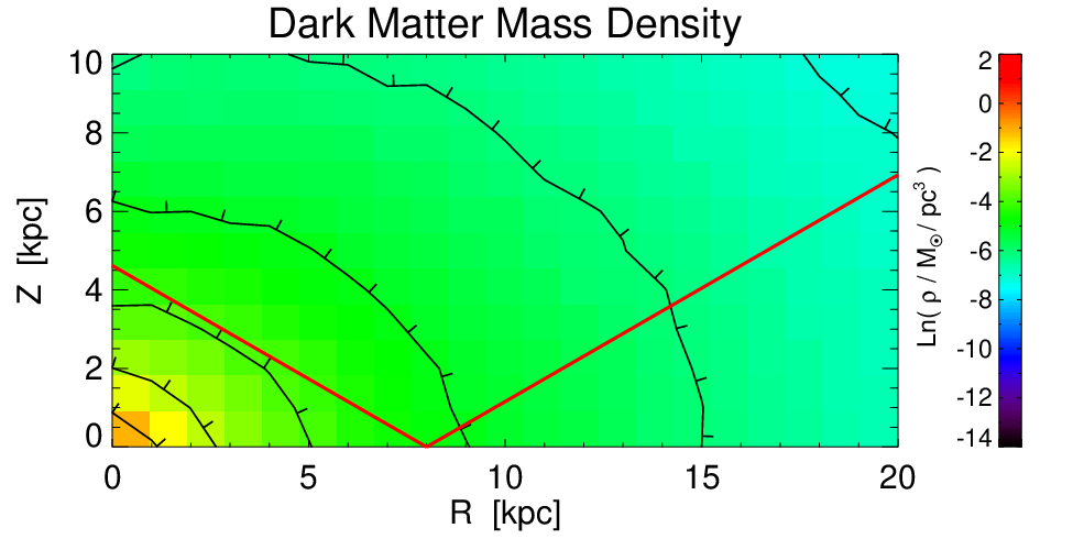
Many of the plots throughout this paper show a total or mean quantity mapped into rectilinear bins in - space within R/kpc and Z/kpc . This perspective gives a sense of the two dimensional distribution of a quantity throughout the SDSS volume. Figure 2 provides an example of this for four relevant quantities within the –body simulation: total, dark matter, visible, and stellar halo mass density. The SDSS footprint within the simulation (shown here in red) is always overplotted for reference. The top left panel of Figure 2 shows the total mass density, including gas, dark matter and stars. To the right of this panel is the dark matter density distribution. The significance of dark matter relative to the gas and stars is not constant, yet the majority of the total mass density within the SDSS footprint is clearly from dark matter. The bottom two panels illustrate the distribution of visible matter. The bottom panel on the left of Figure 2 shows the mass density of all gas and stars within the –body simulation. Two striking structural features stand out within this total visible matter density map: the bulge (R kpc, Z kpc) and disk ( kpc R kpc, Z kpc). These structures are not significantly sampled by the SDSS volume within the simulation. The bottom right-hand panel of Figure 2 shows the stellar halo mass density within the simulation. Note that the majority of the visible mass within the SDSS footprint is from the stellar halo.
II.1.2 Tests of Axial Symmetry
Before we project mean quantities in the - spatial grid or use the axisymmetric form of Jeans equations, we motivate the application of these techniques by illustrating the simulation’s symmetry. The top panel of Figure 3 shows the major to semi-major axis ratio () of dark matter and halo star particles across the SDSS footprint within the simulation. Axis ratios of the particle distribution are determined following the iterative technique outlined in §4.2 of Roškar et al. [68], which identifies isodensity contours. This procedure is analogous to that used in Katz [45], though it uses differential shells (in increments of 0.5 kpc) instead of cumulative shells, following Debattista et al. [25]. For both dark matter particles and stellar halo particles, the axis ratio is always greater than or equal to and less than , indicating the distributions are nearly but not completely axisymmetric in the direction. At the virial radius, the axis ratio for all particles is . The bottom panel of Figure 3 is analogous to the top panel but for the major to minor axis (). The axis ratio is a measure of the departure from spherical symmetry for axisymmetric shells. A axis ratio of 1 is a perfectly spherical mass distribution; indicates that the distribution is flattened (oblate) in the same sense as the stellar disk. At the virial radius, the axis ratio for all particles is . As the bottom panel of Figure 3 shows, in this –body simulation, both the dark matter and stellar distributions are oblate, and the dark matter axis ratio does not vary significantly over the entire SDSS volume.
II.1.3 The Acceleration Maps for a Simulated Galaxy
One final thing to consider before we apply Jeans equations to the simulation: what do the true accelerations look like for the simulation? The top panel of Figure 4 shows the mean component of the acceleration in the direction projected into the - grid; here, the acceleration of each particle was calculated using the force from all the particles in the entire simulation. For comparison, the middle panel shows an analogous map, but here, the acceleration of each star and gas particle was calculated using only the contributions from other star and gas particles (that is, the contribution from the dark matter was not included). As evident, there are substantial differences in the morphology of the two maps; the bottom panel shows the ratio of the top and middle panel. This panel demonstrates that the effect of dark matter on the acceleration in the direction increases quickly away from the plane of the disk and towards the outer parts of the galaxy; for example, the ratio of accelerations is doubled by =8 kpc and =6 kpc. These distances are probed by SDSS – hence these results suggest that the effect of dark matter on stellar acceleration may be uncovered in SDSS data, and that stellar populations in the halo are more sensitive to the existence of dark matter than disk stars.
Along the same lines, the top panel of Figure 5 illustrates the mean component of the acceleration in the direction when the force of all the particles (gas, dark matter and stars) in the simulation is considered, while the middle panel shows the mean component when the force of just gas and star particles are considered. The bottom panel shows a ratio of the top panel to the middle panel; the effects of dark matter are easily discernible; for example, the ratio of accelerations is doubled by =8 kpc and =4 kpc.
II.2. SDSS-based Mock Catalogs: galfast
When constraining the Galactic potential via Jeans equations with SDSS (or any other survey) data, several preliminary analysis steps are required:
- 1.
In order to quantify the stellar number density distribution as a function of coordinates and ( in Equations 1 and 2), the appropriate stellar population needs to be selected (e.g. halo stars), the distances to the stars need to be estimated, and the observational selection function accounted for. In addition, the assumption of cylindrical symmetry must be tested, and the impact of local substructure (e.g. stellar streams) quantified.
- 2.
In order to quantify the four velocity dispersions and the mean azimuthal velocity as functions of coordinates and , complex kinematics (proper motion and radial velocity measurements) are needed and require substantial analysis. For example, the error dependence for the radial velocity components and the error dependence for the tangential velocity components are fundamentally different as a function of distance. Notably, the tangential velocity components are computed as the product of distance and proper motion measurements, and these errors carry their own hidden dependence on distance. Proper motion errors increase for faint stars, and more distant stars are generally fainter than closer ones.
These tasks are far from trivial, but fortunately they have already been undertaken and published.
II.2.1 The Stellar Number Density Distribution for Halo Stars
J08 accomplished the first task of quantifying the stellar number density distribution for both disk and halo components. They showed that the stellar number density distribution, , can be well described (apart from local overdensities) as a sum of two cylindrically symmetric components
| (3) |
The disk component can be modeled as a sum of two exponential disks (see their Equations 22 and 23), while the halo component requires an oblate bi-axial (cylindrically symmetric) power-law model
| (4) |
Here is the local solar neighborhood density of tracer stars, and measures the local fractional contribution of halo stars. The number count normalization, , reflects how tracer stars are selected, and is related to the local luminosity function. Since the overall normalization of in Equations 1 and 2 cancels out, is not of further interest in this context.
J08 obtained best-fit MW parameters using SDSS data, after accounting for selection effects and masking regions with prominent substructure; their results are listed for both the stellar disk and stellar halo components in their Table 10 (second column). For completeness, they obtained , , and , with estimated uncertainties of 25%, 0.1, and 0.2, respectively. We note that the best-fit values for and are covariant – the more symmetric halos correspond to larger , see their Figure 22. They also tested for cylindrical symmetry (see their Figure 11) and could not reject their best-fit axisymmetric number counts model.
I08 studied the metallicity distribution of disk and halo stars and, of direct relevance to this work, demonstrated that the multi-component (i.e. disk and halo) decomposition of from Equation 3 is not a case of over-fitting; instead, a fairly simple selection, , clearly separates disk and halo components (see their Figures 5 and 9) and justifies the decomposition model from Equation 3.
II.2.2 The Kinematic Behavior of Halo Stars
B10 performed a detailed analysis of available kinematic data for the SDSS stellar sample: radial velocities were derived from the SDSS spectroscopic survey and proper motions were obtained by comparing SDSS astrometry and Palomar Observatory Sky Survey astrometry [57] from 50 years earlier. Their main result of interest to this work is a clear demonstration (see their Figures 12 and 13) that the velocity ellipsoid for halo stars is invariant in spherical coordinates within the volume probed by SDSS data (galactocentric distances of 20 kpc). The very complex behavior of measured proper motions (see their Figure 14) and radial velocities (see their Figure 15) on the sky can be explained with a simple triaxial velocity ellipsoid that is invariant in spherical coordinates, =141 km s-1, =85 km s-1, and =75 km s-1, with uncertainties of about 5 km s-1. Their leading sources of uncertainty are distance scale errors, local standard of rest errors, and systematic errors in radial-velocity and proper-motion measurements; see their section 5.3 for details. Given the velocity ellipsoid in spherical coordinates, it can be transformed to cylindrical coordinates as
| (5) |
| (6) |
and
| (7) |
where .
II.3. The galfast Code
The best-fit from J08 and the best-fit velocity ellipsoid for halo stars from B10 can be inserted analytically into Equations 1 and 2 to compute and . Such analytic results properly account for the SDSS selection function and Galactic substructure. However, this approach does not include the effects of finite stellar counts, counting noise, and volume edges. Such sampling effects play an important role in the analysis of the –body simulation, where we utilize numerical derivatives of the “observed” velocity ellipsoid and impose strict stellar count criteria.
To leverage the computational methods developed and tested in the –body framework, we instead generate a mock catalog of SDSS stars generated by the code galfast [42] . This public55 5 See https://github.com/mjuric/galfast Monte Carlo code is based on the best-fit parameterizations of the distributions of stellar number density, metallicity and kinematics constrained by the SDSS data mentioned above. It produces catalogs with the same behavior of observables (such as counts, magnitudes, colors, proper motions, radial velocity) as seen in SDSS data, except that there are no effects of substructure, and selection effects are easily accounted for (e.g., one can generate a mock catalog for the whole Galaxy, and then apply exactly the same selection criteria to this mock catalog and to the –body simulation). The code also generates appropriate error distributions of all measured quantities.
We note that there are no hidden inputs, such as star-formation history, age-metallicity relation, etc., included in galfast – it is simply a sophisticated Monte Carlo generator designed to produce a snapshot of the current sky with the stellar content consistent with SDSS observations.
Using galfast, we generate a flux-limited catalog with and mimic the SDSS sky footprint by only considering high Galactic latitudes (). The catalog lists true positions, absolute magnitudes, velocities and metallicity, as well as corresponding simulated SDSS observations convolved with measurement errors.
We treat this mock catalog as we would treat any catalog downloaded from the SDSS Data Release site. We correct the magnitudes in each filter for interstellar dust extinction and select a halo-like sample using a color cut . The only instance where we use the “truth” provided in the mock catalog is when rejecting stars with to minimize contamination by giants (in a real sample, one could envision obtaining a spectrum for each star to accomplish the same step). The resulting sample of 0.61 million stars is dominated by low-metallicity main sequence F stars, with kinematics commensurate with a halo-dominated sample.
II.4. Numerical Procedures
We process our mock catalog from galfast and our mock catalog from our adopted –body simulation in exactly the same way, using the same code: for a set of stars with given three-dimensional positions and three-dimensional velocities, we first determine the density, , and the five kinematic quantities utilized in Equations 1 and 2, and then compute and .
The computation of the number density, mean azimuthal velocity and velocity dispersions is done for each bin in the - plane. 66 6 In the case of the –body simulation, we also calculated these quantities in 45∘ slices in , rotated in increments of 90∘ from 0 to 360; we found that our results varied no more that 10. We set the bin width to be 1 kpc, and we require at least 100 stellar particles per bin to minimize the shot noise. All quantities are computed using weights proportional to the mass of each stellar particle (assumed constant in the galfast catalogs).
To estimate the gradients required in Equations 1 and 2 (i.e. the spatial gradients of the velocity dispersions and the stellar number density) we use a parametric technique: we fit a second-order polynomial in and to values from the bin being processed and its 8 adjacent neighbors (using IDL fitting routine MPFIT2DFUN), and determine and gradients by taking the analytic derivative of the best fit. This method filters numerical noise (due to counting noise and polynomial fitting) to some extent and produces smoother maps (with values closer to the truth in the galfast catalogs, where we know that velocity dispersion gradients in spherical coordinates are vanishing by construction). We exclude edge pixels (bins) from further analysis because the parametric results are not as robust due to the smaller number of adjacent pixels.
II.4.1 Tests of Numerical Procedures
The galfast catalogs provide a strong test of our algorithms; we have verified that we can recover the number density and kinematics used as input to galfast. Furthermore, we can test the resulting acceleration maps by directly taking appropriate spatial derivatives of the analytic expressions for the spatial distribution from J08 and kinematics from B10 (that is, we can bypass the galfast step). Since these derivatives (“analytic” maps) can be evaluated with negligible numerical noise, unlike derivatives based on a mock sample (“numerical” maps), we can measure the bias and scatter due to a finite-size sample (to the extent that analytic expressions from J08 and B10 are correct, these analytic maps represent ground truth; for their illustration and further discussion see §IV).
A comparison of the analytic and numerical maps reveals that they are morphologically very similar; we find that the latter are biased low by 3% for the maps and by 14% for the map, with a root-mean-square scatter of 25% (over all the pixels) for both maps. This performance is satisfactory for testing the applicability of Jeans equations to a realistic –body simulated galaxy. However, at the smallest Z (2.5 kpc), the map is biased low by as much as a factor of 1.5 at kpc. This biasing is probably due to edge effects when fitting polynomials, or due to insufficient curvature in the fitting functions. When comparing our results to related published work (see §IV) we use the analytic maps, and when comparing mock stellar samples from the –body and galfast simulations we use the numerical maps.
In the case of the –body simulation, we have an additional test: if all algorithms are correctly implemented, and if all assumptions that go into the derivation of Jeans equations are not too incorrect, then we ought to be able to reproduce the true and that are known from direct force calculations. This analysis is described in the following section.
III. Validation of the Jeans Equations Method
In this section we first test the Jeans equations approach using a realistic MW-like simulated galaxy with known stellar accelerations from force computations. The simulated galaxy is not perfectly cylindrically symmetric, nor is it in a steady-state. The comparison of known accelerations and those computed by Jeans equations provides a quantitative assessment of both systematic and random errors inherent in this method. After quantifying these errors, we apply the same methodology to the galfast catalog and demonstrate the signature of dark matter in the Milky Way halo.
III.1. Tests of the Jeans Equations Method Using Simulations
To quantify acceleration errors in the Jeans equations method, we use an –body simulation, with positions, velocities, and accelerations for million stellar particles within the virial radius. To maintain identical selection effects as with the SDSS data, we only use simulation data within the SDSS footprint; this region contains 220,000 stellar particles; their distribution is shown in Figure 6. We include all the star particles from this region in our analysis (that is, there is no specific selection of “halo stars”); however, we exclude results within 1 kpc of the plane of the disk to minimize the influence of disk stars and their strong gradients in all relevant quantities.
Our data is binned in 1 kpc square - pixels; we also investigated smaller bin sizes, down to twice the force softening length (346 parsec). Because the star particle number density decreases quickly with increased galactocentric radius, the adopted size of 1 kpc is a “sweet spot” that allowed us to spatially resolve gradients in the acceleration map, while simultaneously having enough stellar particles per bin for counting errors to remain small (10%).
The top panel of Figure 7 shows the acceleration map generated by applying Jeans equations to the particles from the –body simulation in the region that mimics the SDSS volume. An overall gradient is easy to see; the magnitude of the acceleration decreases with increased radius (). The true acceleration map (shown in the top panel of Figure 4) displays similar behavior; the bottom panel of Figure 7 shows a ratio of the top panel of Figure 7 and the mean true accelerations from the top panel of Figure 4. We find that Jeans equations reproduce the true map quite well: for the entire SDSS volume, the mean value of is with a dispersion77 7 Instead of using the classically defined standard deviation, which is sensitive to non-Gaussian outliers, we use the interquartile range of the distribution to estimate the dispersion. The interquartile range is normalized to obtain a standard deviation in case of Gaussian distribution, , where and are the 25% and 75% quartiles. For more details see Ivezić et al. [37]. of . When we consider a column of data that is unaffected by the bulge in the simulation ( Rkpc ), we find that drops to , with a mean of .
Figure 8 shows an analogous set of maps for acceleration in the direction, . The mean value of the ratio for the entire SDSS volume is with of . When the map is subselected to include data within Rkpc , the mean value drops to with . We note that we tested for the effects of non-axisymmetry on these results by making 8 slices in of 90 degrees offset by 45 degrees. We found that the mean acceleration within these slices varied by around .
We conclude from this analysis of the –body simulation that even in a non-steady state system with deviations from axial symmetry, Jeans equations can still recover meaningful average accelerations; within a given bin, an individual acceleration value has expected random error below 20%, with a bias below 10%. As we show next, this performance is sufficient to enable tests for the existence of dark matter in the MW halo.
III.2. Application of the Jeans Equations Method to SDSS Data
In this section we apply Jeans equations to a catalog of stars from the SDSS volume generated using galfast. We first assess the relative significance of each term in Jeans equations as a function of and to understand the global distribution of and , the components of the acceleration in the and directions implied by the SDSS data. We compare the resulting and maps to the maps generated using the –body simulation; we inspect the morphology of the acceleration maps to draw conclusions about the presence of dark matter within the SDSS Galactic volume.
III.2.1 The Construction of the Acceleration Maps
We first examine the spatial distribution of stars with and (top left panel in Figure 9). A selection function correction has been applied to compensate for the varying range of the axial () angle sampled by the SDSS Galactic data; the computed distribution is a good match to the analytic model used by galfast and verifies that the binning algorithm and the selection function correction are correctly implemented.
Figure 9 also shows velocity distribution moments , , 2, , and . The strong variation with and seen for , , and is due to the use of the cylindrical coordinate system. We have verified that analogous estimates performed in the spherical coordinate system reproduce the spatially invariant velocity ellipsoid used by galfast to within numerical noise.
The spatial derivatives of these terms are used in Equations 1 and 2 to compute and ; they are illustrated in Figures 10 and Figures 11, together with the main result of our analysis, and maps shown in the top left panel in each figure. In each figure, the other panels show all the additive terms from Equations 1 and 2. Note that different terms have varying contributions towards the final acceleration maps. All terms contributing to acceleration maps show smooth global behavior, with only a small number of pixels deviating from the overall trends.
III.2.2 The Initial Interpretation of the Acceleration Maps
Now that we have maps for and , we consider what these maps tell us about the underlying distribution of matter within the SDSS volume. To assess this, we again draw upon our –body simulation to predict what behavior we would expect when the dark matter contribution is and is not included (in §IV, we continue this discussion using a baryon potential derived from SDSS measurements for disk stars).
Recall the top panels of Figures 4 and 5, which shows the map of and from –body simulation. In this case, the acceleration of each particle was calculated using the force from all the particles in the entire simulation. For comparison, the middle panels of these two figures show analogous maps, but there the acceleration was calculated without including the dark matter contribution.
Similarly, the middle and bottom panels of Figures 12 and 13 show the ratio of the and map to the simulation’s and and and maps respectively. Clearly, the acceleration maps derived from the SDSS data are closer to the model-based acceleration maps that include contributions from both baryons and dark matter. At large galactocentric distances, the SDSS accelerations are as much as three to four times stronger than those predicted by a non-dark matter model!
Therefore, by generating acceleration maps using the SDSS data and comparing these maps to expectations from an –body simulation, we have demonstrated that a model containing dark matter is a much better fit to observations than the model that contains baryonic matter alone. While it is encouraging to see yet another aspect of –body simulation that at least qualitatively agrees with data, this far-reaching conclusion can be derived without a reference to simulation, as we show next.
IV. Constraints on the Dark Matter Gravitational Potential
The analysis in the previous section shows that our Jeans equations approach can successfully recover stellar accelerations in a non-steady-state and non-cylindrically symmetric –body simulation. A comparison between the –body simulation and the SDSS-based acceleration maps strongly suggests that a dark matter component is needed to account for the observed accelerations. However, the strength of this conclusion depends on how well the –body simulation matches the observed MW. To supplement our earlier argument, in this section we perform an analysis of the observed acceleration maps that does not require the use of the –body simulation. Instead, we utilize a new observationally constrained description of the MW gravitational potential; we quantitatively compare this potential to our SDSS-based acceleration maps to draw conclusions about the dark matter potential. Because our galfast-based acceleration maps suffer from numerical noise (recall §II.4), here we use the “analytic” acceleration maps computed directly using Equation 4 from J08 and the velocity ellipsoid for halo stars from B10 (see Equations 5–7).
IV.1. Analytic SDSS Acceleration Maps for Halo Stars
Our analytic acceleration maps are shown in Figure 14. As already implied in §II.4.1, they are morphologically very similar to numerical maps shown in the top panels in Figures 12 and 13 (for ease of comparison we used the same - grid although the analytic maps can be evaluated on an arbitrary grid). Although these analytic maps are formally noise-free, as we demonstrated in the preceding section, we anticipate that the random errors due to deviations from cylindrical symmetry and steady state can be up to about 20% (with a bias below 10%).
We find that these maps cannot be described by a spherically symmetric potential. Case in point, there is a large class of potentials of the functional form
| (8) |
For this class, the isopotential surface axis ratio can be estimated as
| (9) |
When we apply the maps shown in Figure 14 to this equation, we find that the median value of is 0.80, with (inter-quartile based) scatter of . This evidence for oblateness comes directly from the fact that the spatial distribution of halo stars is oblate (; see Equation 4). Nevertheless, it does not follow immediately that the dark matter potential must be oblate because the contribution of disk baryons to the potential is non-negligible. We now turn our attention to a recent model where the disk baryons have been carefully accounted for.
IV.2. SEGUE G Dwarfs and the Bovy-Rix Potential
Recently, Bovy & Rix [11, henceforth, BR13] studied in detail the dynamics of 16,000 G dwarfs drawn from the SDSS Sloan Extension for Galactic Understanding and Exploration [89, hereafter SEGUE]. The SEGUE G dwarf sample is dominated by disk stars and extends to 3 kpc from the Galactic plane, with a similar extent in the radial direction [14]. As Bovy et al. [12] show, these disk stars can be separated into sub-populations based upon chemical abundance parameters ( and ). Bovy et al. [12] find that the spatial distribution of each sub-population is well fit by a single exponential profile, both as a function of height above the midplane and galactocentric radius. Moreover, the kinematic behavior of each sub-population is relatively simple [13], making it possible to fit a three-integral action-based distribution function and parametrize the MW potential to the SEGUE data [82, BR13].
BR13’s parametrization of the MW potential includes a two-component gravitational potential, corresponding to the baryon and dark matter content. The former is likely the most robust and precise determination of the MW baryonic potential to date. Additionally, the local normalization for the dark matter component is consistent with a more direct measurement from Bovy & Tremaine [15] and has a similar precision. However, due to the relatively local nature of their sample, BR13 cannot strongly constrain deviations from spherical symmetry for the dark matter model, and thus for this component they adopt a spherically symmetric potential. We note that BR13’s potential model is publicly available via the galactic and MW dynamics python package galpy88 8 See http://galpy.readthedocs.org/en/latest/.
In Figure 15 we explore the accelerations predicted by the BR13 potential model. The top left and right panels of Figure 15 show the and acceleration maps generated from the BR13 baryon potential. We also consider the relative significance of the baryon potential to the dark matter+baryon model; the bottom left and right panels of Figure 15 show the fractional contribution of the baryons to the dark matter+baryon accelerations. These panels include contours of constant fraction. In the case of (bottom right), at kpc the contours are roughly horizontal (parallel to the axis), and in the case of (bottom left), at kpc the contours are relatively more perpendicular. Encouragingly, these trends are in qualitative agreement with the predictions from the –body simulation (see bottom panels in Figures 4 and 5).
We next compare the accelerations predicted by the BR13 two-component potential model to our SDSS-based analytic acceleration maps. Our goal is to understand how well the two-component model, containing a spherically symmetric dark matter halo, fits our SDSS-based results. We begin by considering the data/model ratio: for the model to be a good match to our data, the median value of the ratio should be roughly 1.0 with a small rms (– on a linear scale). In both the cases ( and ), to achieve a median data/model ratio of 1.0, we must rescale the model by multiplying by 0.66 and 0.57 respectively. After these renormalizations, the rms scatter is fairly small (23% on a linear scale). However, because the model derived and require different renormalizations, and there are systematic deviations as functions of and , we conclude that the data versus model discrepancy cannot be resolved by a simple rescaling alone.
To re-emphasize this point, we draw upon an illustrative example. At kpc, kpc, the extrapolated BR13 model predicts and (in units of km/s2) resulting from the dark matter component, and and from baryon component. However, at this location the measured SDSS-based accelerations are and . That is, the model dark matter component by itself exceeds the total measured acceleration.
In contrast to this, we consider in the solar neighborhood at small ( kpc, kpc). Here our SDSS-based acceleration is km/s2. Converting this to an equivalent surface density yields 65 /pc2, with an uncertainty of 10%. This value agrees within errors to the constraints on the equivalent surface density presented in Bovy & Tremaine [15]: using Figure 1 from Bovy & Tremaine [15], the surface density correction factor is 0.9 at kpc, yielding a predicted surface density of 779 /pc2. Hence, the SDSS-based derived from our halo sample is 16% smaller than the acceleration based on disk sample at kpc, kpc, but the two values are consistent within quoted statistical errors.
In summary, our acceleration maps are statistically consistent with [15] at as small as 3 kpc; additionally, we explore much larger galactocentric distances which allows us to draw new constraints on the dark matter potential. However, we note that the extrapolation of our acceleration maps for halo stars to kpc predicts weaker acceleration than experienced by disk stars (as summarized by the BR13 model); we return to this discussion in §VI.1.
We now generate model maps in better agreement with the data by including two modifications to the original BR13 model: 1) we allow for a renormalization of the baryonic component (which is much better constrained than dark matter component, in both shape and amplitude, and thus we expect a renormalization factor close to unity), and 2) we allow departures from spherical symmetry for the dark matter component (as motivated by disagreements at large galactocentric radii).
IV.3. Modified BR13 Potential
Henceforth, we adopt the following description for the gravitational potential used to generate the model acceleration maps
| (10) |
where is the component due to baryons (stars and interstellar medium), is a renormalization factor (discussed in more detail below) and is the component due to dark matter (e.g., see Equation 2-54a in Binney & Tremaine 8),
| (11) |
The free model parameters are , the dark matter potential scale (), the spatial scale (), and the dark matter axis ratio (). Given , we compute and .
IV.4. The Best-fit Dark Matter Potential
Next we discuss our procedure for identifying the best-fit parameters in Equation 10 and Equation 11. We first fix , and exhaustively explore the two-dimensional – parameter space. For a given trial pair of , , we determine the best-fit value for . To do this, we directly compute the data/model ratio for a list of values. The that corresponds to a median data/model ratio of 1.0 is selected as the best fit value of for that particular , pair. There is no a priori guarantee that the corresponding data/model ratio will equal 1.0 as well; however, deviations are minor in practice (1%; this agreement implies that the chosen model form is satisfactory).
Adopting the best for each , pair, we then track the goodness of the , fits by measuring the robust “residual metric.” This metric is defined as the sum of the two ( and ) median absolute deviations; smaller values correspond to better fits (that is, we do not assume the modeldata differences follow a Gaussian distribution).99 9 For completeness, we tried a residual metric that only includes or , to constrain the dark matter potential, but we find that these constraints are much weaker than when both datasets (maps) are considered together. We define the deviation as =log10(data/model) for both maps.
The variation of is shown in the left panel in Figure 16. The plausible (i.e. , not strongly excluded) range for the spatial scale, , is ; outside this range the residual metric rapidly increases to statistically implausible values (given its minimum attained value). The formal (but very shallow) local minimum is found at and , corresponding to km/s. We find that the best-fit values of and are strongly covariant and related via km/s. The axis ratio for the dark matter potential is strongly constrained to the range , and is essentially independent of the choice of .
Now that we have determined our best-fit and parameters, we examine the (data/model)best-fit residuals. In Figure 17, we show the residual (data/model)best-fit maps for and . Allowing for a non-spherical dark matter potential greatly improves the agreement between the data and the model in both cases: the rms scatter is 5% for and 3% for , whereas there was a 23% scatter and need for differing renormalization factors for the original model. As can be seen in the right panel of Figure 17, the largest discrepancy between the data and the best-fit model (shown in dark blue) is found at small , where we know that our map is biased by 16% relative to the BR13 results. In the left panel of Figure 17, the largest discrepancy between the data and the best-fit model (shown in red) is found at the smallest and large , with measured acceleration 1.8 times larger than the best-fit model value. We conclude that either one of the two adopted SDSS results from J08 or B10 is problematic in this region, or that the adopted model potential is incapable of fully explaining observations. We continue this discussion in §VI.1.
IV.4.1 The Impact of Uncertainty in on Other Quantities
As noted above, our constraints on are weak (e.g. , is plausibly within ). Here, we investigate if relevant local measurements can strengthen our constraints on and provide a check for our best-fit dark matter potential.
Before we can utilize any local mass measurements, we must convert our analytic gravitational potential to a mass density distribution. Fortunately, [8] provides the following expression for converting to matter density (see their Equation 2-54b) from a gravitational potential of the functional form described by Equation 11,
| (12) | |||
Using this expression with our best-fit values of , , and km/s, we obtain = 0.004 , with an estimated uncertainty of only about 10% due in large part to our uncertainty in . This estimate is within statistical agreement with the result of from Bovy & Tremaine [15].
As discussed in [8], when , the density distribution predicted by Equation 12 is negative near the axis for . However, this unphysical behavior is of no concern here because kpc even for the smallest allowed , which is clearly far beyond the probed volume.
For the small relevant here, the isodensity contours are elliptical with the axis ratio given by
| (13) |
yielding = 0.36. This result is in good agreement with the estimate from [53], but we note that the baryon contribution to the potential was not accounted for in their study and thus it is superseded by the above result.
We also consider the dark matter contribution to the local circular speed, which can be computed from (see Equation 2-54c in Binney & Tremaine 8)
| (14) |
Considering the plausible range of (), we estimate to be km/s via a linear fit. Our best-fit value, km/s, is uncertain to within 3 km/s (again, due to the weak constraints on ). Thus, we find that considering the local circular speed does not provide a strong constraint on .
The best-fit contribution of dark matter halo to the local circular speed, km/s, is a factor of two smaller than that estimated by BR13. This discrepancy probably implies that the adopted logarithmic potential given by Equation 11 close to the Galactic plane does not have sufficient curvature in the direction to produce larger (the normalization cannot be responsible because it’s value is set by distant halo stars). A similar “curvature problem” close to the plane (and close to the symmetry axis) with J08 and B10 results is discussed in §VI.1.
IV.5. The Uniqueness of Adopted Dark Matter Potential
At large galactocentric radii the dark matter contribution to the force felt by halo stars dominates over the baryon contribution. Measurements are precise enough to test whether functional forms other than the adopted logarithmic potential given by Equation 11 would fit the data.
We first test whether a single value of is sufficient: using Equation 9, but this time with the BR13 baryon contribution subtracted from the measured maps, we find that the median value (per bin) of is 0.67, with (inter-quartile based) scatter of . The small width of the distribution indicates that the spatial variation of the acceleration maps is well captured by the variable given by Equation 8.
It is straightforward to show that for a generalized potential
| (15) |
where is given by Equation 8,
| (16) |
For the logarithmic potential, , deviations from a logarithmic potential will be seen as deviations of the first two terms from the expected behavior. For the region with kpc and kpc, we find no evidence of the departures from a logarithmic potential.
Nevertheless, the dynamic range of is fairly small, from 3.5 to 4.5 for kpc, and for a power-law potential, , can provide a very good description of the best-fit logarithmic potential, especially if is re-fit. With kpc, provides almost the same potential (with per bin scatter of 0.2%) as the best-fit logarithmic potential (that is, 2 ln(x) is very close to 1.007 x0.73 for ). When is changed to 22 kpc, the agreement is even better with a best-fit . Forcing does not provide a satisfactory fit for any . Therefore, while a logarithmic potential is fully consistent with the data, it is not a unique solution. The main reason for this ambiguity is the small dynamic range of due to the finite sampled volume. We reiterate that is robustly determined irrespective of the detailed form for .
IV.6. Test of the BR13 Baryon Potential
In our analysis above, we assumed that the baryon component in the BR13 potential is perfect (). We now relax this assumption and allow and to be free fitting parameters, with a fixed kpc.
Our resulting variation in is shown in the right panel in Figure 16; we find the best-fit values (shown in dark blue) to be , . Although the formal best fit is found at , the data are fully consistent with . Based on the variations of best-fit with other fitting parameters, we conclude that its formal uncertainty is much smaller than 0.1. However, due to plausible deviations between the adopted analytic potential and reality, and departures from steady state and cylindrical symmetry, we cannot exclude the possibility that its systematic uncertainty could be as large as 0.1. Hence, we adopt as our best-fit model and a logarithmic dark matter potential with , kpc and km/s.
IV.7. The Impact of Uncertainty from the J08 Best-fit Parameters
The upper limits on the uncertainty of the best-fit halo parameters quoted by J08 are 0.2 for and 0.1 for (see their Table 10 and discussion in § 4.2.4). The formal uncertainties in fitting (based on a analysis) are several times smaller. These two parameters are highly covariant (see figure 22 in J08); values of that are larger than the best-fit value (i.e., a steeper halo stellar number density profile) correspond to larger values of , and vice versa.
When the parameter values for the stellar halo are varied from (=2.57, =0.54) to (=2.97, =0.74) along the direction of covariance, the resulting (potential) varies from 0.55 to 0.82, with the implied varying from 0.19 to 0.57. Because the adopted variation in and represents an upper limit, we conclude that our final errors of 0.1 for and are not dominated by uncertainties in the best-fit values for and .
IV.8. Comparison with Other Results
This is the first study where distant halo stars have been used to constrain the shape of dark matter potential in situ at galactocentric distances of up to 20 kpc. However, related constraints on have been obtained in studies of stellar streams, most notably using the Sagittarius dwarf tidal stream [52, e.g.,] and the GD-1 stream (see below). The former provides constraints at much larger galactocentric radii (20-50 kpc) than considered here and thus we focus below on the analysis of GD-1. We note that Vera-Ciro & Helmi [85] used the Sagittarius dwarf tidal stream to constrain the dark halo potential and found that within 10 kpc from the Galactic center it is axisymmetric and flattened toward the disk plane with .
IV.8.1 Tidal Stream GD-1
GD-1 is a long, thin stellar stream discovered in SDSS DR 4 photometry in 2006 [31]. GD-1 spans across the northern sky, passes within 30∘ of the Galactic pole, and is at its midpoint about 8 kpc away from the midplane of the disk [21]. Based upon the SDSS photometry, USNO-B astrometry, and SEGUE spectroscopy, Koposov et al. [49, hereafter K10] were able to construct an empirical six-dimensional phase-space map of the stream.
From their analysis, K10 conclude that GD-1 is on an eccentric orbit that is consistent with a single flattened isothermal potential. That is, K10 fit GD-1 using a model of the same functional form as Equation 11, but they suppose it accounts for both baryons and dark matter. In this limit, K10 adopt and conclude that the total axis ratio, , is equal to .
To emulate K10’s results, we have repeated our fitting procedure with a fixed (that is, supposing no separate baryon component to the potential). We find that in this case, is indeed strongly preferred, and we obtain , which is consistent with the K10 results.
K10 go on to estimate by including a simple baryon bulge+disk model in their analysis; from this, they find a lower limit on ( at the 90% confidence level). This lower limit appears to exclude our best-fit value; however, the differing results are not surprising given the fact that their baryon model is significantly different than ours. It is likely that the baryon component determined by BR13 is much more robust than the model used by K10. We reiterate that when using the same functional form for the potential, we get the same best-fit model parameters as K10. Thus, in an indirect sense, the accelerations measured by halo stars are consistent with the potential needed to explain observations of the GD-1 stream.
It is certainly surprising that a single-component potential can provide a good description of acceleration maps for halo stars, especially given the complex morphology of the B13 baryon component (see the top panels in Figure 15). We consider this in further detail by comparing our best-fit two-component model with a single-component model. The ratios predicted for the and maps are shown in the left and right panels of Figure 18 respectively.
As can be seen in both panels of Figure 18, above 3-4 kpc, the two models agree quite well (shown in green and matching to within 10%). This, in fact, is the region where most of constraints from both the K10 analysis and our analysis come from. However, given the kpc constraints from BR13, it is clear that a single-component model does not have the flexibility to explain simultaneously both the BR13 SEGUE G dwarfs data and our SDSS halo stars data. For example, at kpc and , the single-component model predicts acceleration that is too small by a factor of 6 compared to the best-fit two-component model and constraints from BR13. We conclude from this that the potential from K10 cannot be extrapolated close to the Galactic plane.
The best-fit model adopted here does not suffer from this problem because close to the plane it is dominated by the baryon component. Nevertheless, recall that the contribution of the dark matter halo to the local circular speed is a factor of 2 smaller than estimated by BR13.
V. Testing MOND
Modified Newtonian dynamics (MOND) is a proposed alternative to dark matter, which posits a breakdown of Newtonian dynamics in the limit of small accelerations [55, and references therein]. When the Newtonian acceleration, , is much larger than a characteristic acceleration scale, , the acceleration felt by a test particle is Newtonian, . However, when , the acceleration felt by a test particle is much larger than the Newtonian prediction, . The characteristic acceleration scale is about km/s2, that is, very similar to the range of accelerations felt by halo stars in the volume probed by the SDSS. In the acceleration range between these two extremes, the acceleration is given by an interpolating function
| (17) |
where . The interpolating function satisfies for , and when . For example, Famaey & Binney [27] investigated functions such as and . The physical basis of MOND theories is discussed in Sanders & McGaugh [70] and Bekenstein [5].
In addition to sampling the relevant range of acceleration, the SDSS data for halo stars simultaneously constrains two components of acceleration and enables a very powerful test of the MOND model. The left panel in Figure 19 shows the ratio of acceleration due to baryons from the BR13 model and the measured acceleration for halo stars as a function of the measured acceleration. MOND models predict that the two should be correlated, and indeed data for each component ( and ) show remarkably small scatter about a mean trend. However, the two trends are significantly offset from each other and it is impossible to fit them both with a single interpolating function. In other words, both the magnitude of the measured acceleration is different than predicted by the baryons, and the direction of the acceleration vector is different. Since MOND modifies only the former1010 10 Strictly speaking, this is true only for Milgrom’s MOND; it might be possible to avoid this problem via the addition of a solenoidal vector field to Newtonian acceleration; see Equation 19 in Famaey & McGaugh [28]., it cannot explain the latter.
For further illustration, Figure 20 shows the variation of the angle between the measured acceleration vector and the acceleration vector predicted by the BR13 model for baryons within the probed volume; this angle is in the range 0∘–10∘, with a median value of 4.7∘. The largest values are found for the largest and ; significantly detected differences between the direction of the measured acceleration vector and the direction of the baryon-based prediction are found for kpc and kpc. For example, at the bin with kpc and kpc, the angle between the measured acceleration vector and the direction towards the Galactic center is 12.5∘, and the angle between the acceleration predicted by the baryon model and the direction towards the Galactic center is 3.2∘ – this is a difference of 9.3∘ (see vectors marked in the figure)! This mismatch angle cannot be explained by MOND; MOND only modifies the length of the baryon prediction but not its direction. For the same reason, a spherical dark matter halo does not work either – its prediction always points directly towards the GC. The vector sum of the dark matter contribution for an oblate halo and the baryon contribution produces a satisfactory model.
To quantitatively estimate the disagreement between our data and MOND models, we have tried three different interpolating functions, , and , where the index in the last one was determined as a free parameter. The corresponding best-fit values of the characteristic acceleration are , and , respectively (in units of 10-13 km/s2). The scatter of data around the model prediction is smallest for the third MOND model, 17%. This scatter is still more than three times larger than for the best-fit model with dark matter from the preceding section, which produces a scatter of 4.8%. The data/model ratio distributions are shown in the right panel in Figure 19. If data for and are treated separately, then the scatter for each can be decreased to about 10%, but the ratio of best-fit values of (using the third model) is significantly different from 1 (0.39 for and 0.27 for ). Because it is impossible to construct a single MOND model that outperforms the model with dark matter, the latter is statistically preferred.
Therefore, thanks to precise two-dimensional measurements of acceleration for halo stars, we can reject the MOND model as an explanation of the observed behavior. The model that incorporates a dark matter halo is in much better agreement with the data. Nevertheless, we emphasize that these conclusions are critically dependent on the accuracy of the baryon potential.
VI. Discussion and Conclusions
We have demonstrated that the SDSS observations of the MW stellar halo combined with the gravitational potential due to baryons derived by BR13, imply the existence of an invisible component that contributes to the overall gravitational potential. At large galactocentric distances (20 kpc), the detection of this component is highly significant and robust because the gravitational force experienced by halo stars is as much as three times stronger than what can be attributed to purely visible matter.
Our results are derived using Jeans equations, which estimate the gradient of the gravitational potential statistically from the observed spatial variation of stellar counts and stellar kinematics (Equations 1 and 2). The derivation of these equations assumes a cylindrically symmetric steady-state system. Both available MW data and –body simulations indicate that these assumptions cannot be fully satisfied and thus the performance of the Jeans equations method must be critically examined before drawing conclusions.
Using a modern cosmologically derived –body simulation, designed to mimic the formation and evolution of a MW–like galaxy, we showed that the Jeans equations method can uncover true accelerations despite deviations from a steady-state system with cylindrical symmetry: we recovered true mean per-bin accelerations with random errors below 20% and a bias below 10%. Such a precision is more than sufficient to robustly detect deviations between the measured acceleration and the acceleration that can be attributed to baryonic material.
When applied to SDSS data, this method produced two-dimensional acceleration maps to heliocentric distances exceeding 10 kpc and galactocentric distances exceeding 20 kpc. It was possible to probe this large distance range thanks to substantial SDSS sky coverage and accurate multi-color photometry to faint limits. Leveraging the baryonic gravitational potential from BR13, we showed that the gravitational force experienced by halo stars at galactocentric distances of 20 kpc cannot be explained, in a Newtonian framework, by only baryon matter contributions. At these large galactocentric distances, the discrepancy is much larger than in the Solar neighborhood because the baryonic material is concentrated in the Galactic disk, while the presumed dark matter is much more extended.
We attempted to construct a MOND model in agreement with the data, but found that our best-fit MOND model is significantly outperformed by a model with dark matter. MOND’s inability to explain the data is related to the evidence for a non-spherical dark matter distribution (which comes from the oblate spatial distribution of halo stars). Specifically, the magnitude of the measured acceleration is different than predicted by baryons, and the direction of the measured acceleration vector is different, too. Since MOND modifies only the former, it cannot explain the latter. Therefore, because of precise two-dimensional measurements of the acceleration of halo stars, MOND models can be rejected irrespective of the details assumed in the interpolating function and the value of the characteristic acceleration. Of course, these conclusions are critically dependent on the accuracy of the baryon potential.
The large volume probed by SDSS halo stars also provides a strong constraint on the shape of the dark matter halo potential. Within galactocentric distances of 20 kpc, the dark matter halo potential is well described by an oblate halo with axis ratio ; this corresponds to an axis ratio for the dark matter density distribution. The quoted uncertainties attempt to account for systematic errors but Gaussian behavior cannot be guaranteed. The formal random errors for and do not exceed 0.05. The parameter in the logarithmic dark matter model, and the preference for logarithmic over power-law model, are not as well constrained as .
The resulting best-fit two-component gravitational potential, based on the baryonic component from BR13, and the dark matter component described by eq. 11, is simultaneously consistent with relatively local (within 3 kpc) measurements of disk stars, and with measurements of halo stars to galactocentric distances of 20 kpc. The best-fit potential derived here is also consistent with the gravitational potential required to explain the spatial and kinematic behavior of the GD-1 tidal stream. Given vastly different selection criteria, spatial distributions and kinematics of these three populations, this consistency is indeed remarkable!
Nevertheless, it is almost certain that the functional form given by eq. 11 cannot be valid throughout the entire MW halo, as we discuss next.
VI.1. The Range of Validity of Our Results
Our analysis is based on both stellar count and kinematics data from the SDSS Galactic catalog, which extends to no more than 20 kpc from the Galactic center. This dataset excludes the vicinity immediately surrounding the Galactic center, as well as the region very close to the Galactic plane (closer than 3 kpc). Therefore, our results should not be extrapolated beyond this limit.
There are already strong indications that the stellar halo model from J08, given by Equation 4, cannot be extrapolated beyond a galactocentric distance of about 30 kpc. [74] found, using main sequence stars detected by the Canada-France-Hawaii Telescope Legacy Survey (CFHTLS) in about 170 deg2 of sky, that the halo stellar number-density profile becomes steeper at Galactocentric distances greater than 28 kpc, with the power-law index changing from to . They measured the oblateness of the stellar halo to be 0.01 (statistical error only), and they detected no evidence of the oblateness changing across the range of distances probed. [24] explored similar issues, using a sample of 20,000 BHB and blue straggler stars detected by SDSS over 14,000 deg2 of sky, and obtained almost identical results to those from [74]. Their best fitting model has an inner power-law index of and an outer index of , with the transition occurring at 27 kpc, and a constant stellar halo flattening of . In addition, the distributions of RR Lyrae stars from the SEKBO survey [47], and of RR Lyrae stars from SDSS Stripe 82 data [87, 75], indicate a steeper density profile beyond 30 kpc. These results are in general agreement with the dual halo hypothesis advocated in [4], and references therein (and also including opposing views).
Similarly, the finding by B10 that the velocity ellipsoid for halo stars is invariant in spherical coordinates cannot be valid beyond about 30 kpc from the Galactic center. [19] used the Hypervelocity Star survey data to measure the halo radial-velocity dispersion out to 75 kpc. They obtained results in statistical agreement with similar studies by [3] and [88], which they summarized as: “the Milky Way radial-velocity dispersion drops from km s-1 at kpc to km s-1 at kpc” (here is the Galactocentric spherical radius in this paper). It is hard to quantitatively and robustly estimate what this gradient implies for the underlying potential because the velocity dispersion in two orthogonal directions at distances beyond 30 kpc has not been measured yet; these measurements will likely have to wait for Gaia and LSST surveys (Ivezić et al. 36, also see below). We note that [85] constrained the dark halo potential using the Sagittarius dwarf tidal stream at a large range of galactocentric radii. They found that the potential is axisymmetric and flattened toward the disk plane within 10 kpc from the Galactic center, with . At larger radii, they argue for a triaxial shape in the outer halo, consistent with the Law & Majewski [52] model, with deviations from oblate halo starting at galactocentric distances of about 10 kpc.
The acceleration of the halo stars in the direction and close to the Galactic plane is weaker than that experienced by disk stars. Figure 21 shows data and models for at kpc and kpc. While at kpc, the agreement between halo and disk star accelerations is satisfactory, at kpc and within a few kpc from the plane, the implied acceleration of halo stars is weaker than that experienced by disk stars, with discrepancy increasing from about a factor of 2 at kpc to larger values at smaller (note that all values vanish at because of symmetry). It appears that either the spatial distribution of halo stars from J08, or kinematics from B10 (or both) has to break down close to the plane. In order to increase the implied acceleration, more curvature, that is, larger derivatives of the spatial distribution and kinematics, are needed close to the plane. With existing data it is hard to quantify what is the problem because the fraction of halo stars is very small close to the plane and it is easy to get sample contamination (this is why B10 only analyzed halo stars that are more than 3 kpc from the plane). Furthermore, turn-off halo stars closer than about 1 kpc are saturated in SDSS imaging.
We can postulate a minor modification of the parameter from eq. 4, from its best-fit value obtained by J08, that brings acceleration component of halo stars in agreement with acceleration of disk stars at kpc. The third term on the right-hand side of eq. 2 is proportional to for small . If decreases from 0.64 at kpc to at kpc, the resulting for halo stars becomes similar to for disk stars. At the same time, the stellar number density given by eq. 4 is insensitive to for and kpc, and thus remains consistent with J08 and B10 analysis. The implication is that the halo is more oblate closer to the disk midplane than far away from it, an idea that was already advocated in the literature (e.g., Preston et al. 66).
It is likely that Gaia will provide a definitive resolution of this puzzle. Gaia will also likely resolve the origin of the divergence of on the symmetry axis (). Because values for and obtained by B10 are different, computed using Equation 1 diverges for (for , ). Proper motion accuracy below 1 mas yr-1 is required to map the behavior of and close to the Galaxy’s symmetry axis.
Figure 21 also illustrates that the dark matter component from the original BR13 model produces too much force at large . This discrepancy is resolved by replacing their spherical dark matter model by the new oblate dark matter model introduced here. While this modification results in a satisfactory explanation for the measured halo star acceleration maps, it fails to produce a sufficiently large dark matter halo contribution to the local circular speed by about a factor of two. This failure suggests that the adopted logarithmic potential given by Equation 11 close to the Galactic plane does not have sufficient curvature in the direction. In other words, the dark matter should be more concentrated toward the plane of the disk the our adopted model predicts.
In summary, these discrepancies indicate that both the dark matter distribution, and the spatial distribution and kinematics of halo stars, should be sensitive to the existence of a stellar disk, but the current models do not capture this behavior.
In addition to the data limitations, simulations have their own caveats. We have demonstrated using an –body simulation that the Jeans equations method can recover the true stellar acceleration with a bias below 10%. However, the general validity of this conclusion is crucially dependent on the similarity between the simulated galaxy and the MW. We showed that the simulated galaxy is similar to the MW in many important ways, such as the overall distribution of halo stars and their kinematics. Nevertheless, there are other untested aspects that might be important and perhaps are biasing our measurements of the dark matter halo properties. For example, [73, 72] have shown, using data from the SDSS SEGUE spectroscopic survey, that about 10% of the halo stars within 20 kpc from the Sun cluster kinematically on very small spatial scales (typical radial-velocity dispersion is 20 km s-1). It remains to be seen whether simulated galaxies also include this effect, and how it affects the performance of the Jeans equations method.
Last but not least, in deriving our conclusions we assumed that the BR13 baryon potential, derived using a sample of disk G dwarfs, is perfect. They directly measured (at =1.1 kpc and 4.5 ) from the vertical dynamics and combined it with from the tangent-point rotation curve measurements. Their model produces equivalent to local circular speed of =220 km/s. Since at this time is uncertain by possibly as much as 10%, a similar level of uncertainty is implied for their baryon potential.
VI.2. Future Work
It is possible to go beyond Jeans equations to use stellar kinematics to probe the full phase space distribution of stars [7, e.g.,]. For example, as Valluri et al. [84] recently demonstrated, stellar orbits can be used to determine not only the shape of the inner halo, but the global shape of the Galactic halo. The Valluri et al. orbital spectral analysis method provides a strong complementary tool to the technique presented here for constraining the potential of the Milky Way halo and its stellar distribution function. In addition, outcomes of methods such as “made-to-measure models” (Syer & Tremaine 81; Dehnen 26), direct modeling of the distribution function [63], and modeling of stellar tidal streams (K10; Bonaca et al. 9) can be compared to constrain systematic errors of each method and improve understanding of the Milky Way mass distribution.
The full potential of these methods will be reached by upcoming next-generation surveys, such as Gaia [62] and LSST [38]. First, Gaia will provide measurements of distances and kinematics with a similar faint flux limit as SDSS, but with much smaller errors (for a comparison of SDSS, Gaia and LSST astrometric and photometric errors, see figure 21 in Ivezić et al. 36). In particular, Gaia data will be superior to currently available data for quantifying the spatial distribution and kinematics of halo stars close to the plane.
LSST will obtain photometric and kinematic measurements of comparable accuracy to those of Gaia at Gaia’s faint limit, and extend them deeper by about 5 mag. With LSST, it will be possible to extend this study to about 10 times larger distance limit than possible today with SDSS data [36]. Most notably, it will be possible to investigate whether the dark matter halo shows any trace of changes in the spatial and kinematic behavior around 30 kpc from the Galactic center that are revealed by halo stars. Furthermore, by extending the limiting distance, the impact of baryons will be diminished and the conclusions about dark matter behavior will be more robust.
VII. Acknowledgments
We thank Monica Valluri, Victor Debattista, and Carlos Vera-Ciro for illuminating discussions. SL and ŽI acknowledge support by NSF grants AST-0707901 & AST-1008784 to the University of Washington. SL acknowledges support from the Washington NASA Space Grant Consortium and Michigan Society of Fellows. ŽI acknowledges support by NSF grant AST-0551161 to LSST for design and development activity, by the Croatian National Science Foundation grant O-1548-2009, and thanks the Hungarian Academy of Sciences for its support through the Distinguished Guest Professor grant No. E-1109/6/2012. JB was supported by NASA through Hubble Fellowship grant HST-HF-51285.01 from the Space Telescope Science Institute, which is operated by the Association of Universities for Research in Astronomy, Incorporated, under NASA contract NAS5-26555. FG acknowledges support from NSF grant AST-1108885. Resources supporting this work were provided by the NASA High-End Computing (HEC) Program through the NASA Advanced Supercomputing (NAS) Division at Ames Research Center. Galfast computations were performed on Hybrid at the Physics Department, University of Split, financed by the National Foundation for Science, Higher Education and Technological Development of the Republic of Croatia.
References
- [1] Bahcall, J. N. 1984, ApJ, 276, 169
- [2] Barnes, J., & Efstathiou, G. 1987, ApJ, 319, 575
- [3] Battaglia, G., et al. 2005, MNRAS, 364, 433
- [4] Beers, T. C., Carollo, D., Ivezić, Ž., et al. 2012, ApJ, 746, 34
- [5] Bekenstein, J. D. 2004, PhRvD, 70, 083509
- [6] Berry, M., Ivezić, Ž., Sesar, B., et al. 2012, ApJ, 757, 166
- [7] Binney, J. 2013, NewAR, 57, 29
- [8] Binney, J., & Tremaine, S. 1987, Galactic Dynamics (1st ed.; Princeton, NJ: Princeton University Press)
- [9] Bonaca, A., Geha, M., Kuepper, A. H. W., et al. 2014, ArXiv e-prints, arXiv:1406.6063
- [10] Bond, N. A., Ivezić, Ž., Sesar, B., et al. 2010, ApJ, 716, 1
- [11] Bovy, J., & Rix, H.-W. 2013, ApJ, 779, 115
- [12] Bovy, J., Rix, H.-W., & Hogg, D. W. 2012a, ApJ, 751, 131
- [13] Bovy, J., Rix, H.-W., Hogg, D. W., et al. 2012b, ApJ, 755, 115
- [14] Bovy, J., Rix, H.-W., Liu, C., et al. 2012c, ApJ, 753, 148
- [15] Bovy, J., & Tremaine, S. 2012, ApJ, 756, 89
- [16] Bovy, J., Allende Prieto, C., Beers, T. C., et al. 2012d, ApJ, 759, 131
- [17] Boylan-Kolchin, M., Besla, G., & Hernquist, L. 2011, MNRAS, 414, 1560
- [18] Brooks, A. M., Solomon, A. R., Governato, F., et al. 2011, ApJ, 728, 51
- [19] Brown, W. R., Geller, M. J., Kenyon, S. J., & Diaferio, A. 2010, AJ, 139, 59
- [20] Bullock, J. S., & Johnston, K. V. 2005, ApJ, 635, 931
- [21] Carlberg, R. G., & Grillmair, C. J. 2013, ApJ, 768, 171
- [22] Christensen, C., Quinn, T., Governato, F., et al. 2012, MNRAS, 425, 3058
- [23] Creze, M., Chereul, E., Bienayme, O., & Pichon, C. 1998, A&A, 329, 920
- [24] Deason, A. J., Belokurov, V., & Evans, N. W. 2011, MNRAS, 416, 2903
- [25] Debattista, V. P., Moore, B., Quinn, T., et al. 2008, ApJ, 681, 1076
- [26] Dehnen, W. 2009, MNRAS, 395, 1079
- [27] Famaey, B., & Binney, J. 2005, MNRAS, 363, 603
- [28] Famaey, B., & McGaugh, S. S. 2012, LRR, 15, 10
- [29] Garbari, S., Liu, C., Read, J. I., & Lake, G. 2012, MNRAS, 425, 1445
- [30] Governato, F., Zolotov, A., Pontzen, A., et al. 2012, MNRAS, 422, 1231
- [31] Grillmair, C. J., & Dionatos, O. 2006, ApJ, 643, L17
- [32] Hogan, C. J., & Dalcanton, J. J. 2000, PhRvD, 62, 063511
- [33] Holmberg, J., & Flynn, C. 2000, MNRAS, 313, 209
- [34] —. 2004, MNRAS, 352, 440
- [35] Ibata, R., Lewis, G. F., Irwin, M., Totten, E., & Quinn, T. 2001, ApJ, 551, 294
- [36] Ivezić, Ž., Beers, T. C., & Jurić, M. 2012, ARA&A, 50, 251
- [37] Ivezić, Ž., Connolly, A., VanderPlas, J., & Gray, A. 2013, Statistics, Data Mining, and Machine Learning in Astronomy (1st ed.; Princeton, NJ: Princeton University Press)
- [38] Ivezić, Ž., Tyson, J. A., Acosta, E., et al. 2008a, ArXiv e-prints, 0805.2366
- [39] Ivezić, Ž., Sesar, B., Jurić, M., et al. 2008b, ApJ, 684, 287
- [40] Jeans, J. H. 1915, MNRAS, 76, 70
- [41] Johnston, K. V., Zhao, H., Spergel, D. N., & Hernquist, L. 1999, ApJ, 512, L109
- [42] Jurić, M., Ćosić, K., Vinković, D., & Ivezić, Ž. 2010, in Bulletin of the American Astronomical Society, Vol. 42, American Astronomical Society Meeting Abstracts #215, 222
- [43] Jurić, M., Ivezić, Ž., Brooks, A., et al. 2008, ApJ, 673, 864
- [44] Kapteyn, J. C. 1922, ApJ, 55, 302
- [45] Katz, N. 1991, ApJ, 368, 325
- [46] Katz, N., & White, S. D. M. 1993, ApJ, 412, 455
- [47] Keller, S. C., Murphy, S., Prior, S., Da Costa, G., & Schmidt, B. 2008, ApJ, 678, 851
- [48] Klypin, A., Zhao, H., & Somerville, R. S. 2002, ApJ, 573, 597
- [49] Koposov, S. E., Rix, H.-W., & Hogg, D. W. 2010, ApJ, 712, 260
- [50] Kuijken, K., & Gilmore, G. 1989, MNRAS, 239, 651
- [51] —. 1991, ApJ, 367, L9
- [52] Law, D. R., & Majewski, S. R. 2010, ApJ, 714, 229
- [53] Loebman, S. R., Ivezić, Ž., Quinn, T. R., et al. 2012, ApJ, 758, L23
- [54] Markevitch, M., Gonzalez, A. H., Clowe, D., et al. 2004, ApJ, 606, 819
- [55] Milgrom, M. 2014, MNRAS, 437, 2531
- [56] Moni Bidin, C., Carraro, G., Méndez, R. A., & Smith, R. 2012, ApJ, 751, 30
- [57] Munn, J. A., Monet, D. G., Levine, S. E., et al. 2004, AJ, 127, 3034
- [58] Munshi, F., Governato, F., Brooks, A. M., et al. 2013, ApJ, 766, 56
- [59] Oort, J. H. 1932, BAN, 6, 249
- [60] —. 1960, BAN, 15, 45
- [61] Peebles, P. J. E. 1969, ApJ, 155, 393
- [62] Perryman, M. A. C. 2002, Ap&SS, 280, 1
- [63] Piffl, T., Binney, J., McMillan, P. J., et al. 2014, ArXiv e-prints, arXiv:1406.4130
- [64] Pontzen, A., Governato, F., Pettini, M., et al. 2008, MNRAS, 390, 1349
- [65] Power, C., Navarro, J. F., Jenkins, A., et al. 2003, MNRAS, 338, 14
- [66] Preston, G. W., Shectman, S. A., & Beers, T. C. 1991, ApJ, 375, 121
- [67] Read, J. I. 2014, JPhG, 41, 063101
- [68] Roškar, R., Debattista, V. P., Brooks, A. M., et al. 2010, MNRAS, 408, 783
- [69] Rubin, V. C., Ford, W. K. J., & . Thonnard, N. 1980, ApJ, 238, 471
- [70] Sanders, R. H., & McGaugh, S. S. 2002, ARA&A, 40, 263
- [71] Scannapieco, C., Wadepuhl, M., Parry, O. H., et al. 2012, MNRAS, 423, 1726
- [72] Schlaufman, K. C., Rockosi, C. M., Lee, Y. S., Beers, T. C., & Allende Prieto, C. 2011, ApJ, 734, 49
- [73] Schlaufman, K. C., Rockosi, C. M., Allende Prieto, C., et al. 2009, ApJ, 703, 2177
- [74] Sesar, B., Jurić, M., & Ivezić, Ž. 2011, ApJ, 731, 4
- [75] Sesar, B., Ivezić, Ž., Grammer, S. H., et al. 2010, ApJ, 708, 717
- [76] Shen, S., Wadsley, J., & Stinson, G. 2010, MNRAS, 407, 1581
- [77] Siebert, A., Bienaymé, O., & Soubiran, C. 2003, A&A, 399, 531
- [78] Smith, M. C., Whiteoak, S. H., & Evans, N. W. 2012, ApJ, 746, 181
- [79] Spergel, D. N., Verde, L., Peiris, H. V., et al. 2003, ApJS, 148, 175
- [80] Stinson, G., Seth, A., Katz, N., et al. 2006, MNRAS, 373, 1074
- [81] Syer, D., & Tremaine, S. 1996, MNRAS, 282, 223
- [82] Ting, Y.-S., Rix, H.-W., Bovy, J., & van de Ven, G. 2013, MNRAS, 434, 652
- [83] Tremaine, S., & Gunn, J. E. 1979, PhRvL, 42, 407
- [84] Valluri, M., Debattista, V. P., Quinn, T. R., Roškar, R., & Wadsley, J. 2012, MNRAS, 419, 1951
- [85] Vera-Ciro, C., & Helmi, A. 2013, ApJ, 773, L4
- [86] Wadsley, J. W., Stadel, J., & Quinn, T. 2004, NewA, 9, 137
- [87] Watkins, L. L., Evans, N. W., Belokurov, V., et al. 2009, MNRAS, 398, 1757
- [88] Xue, X. X., Rix, H. W., Zhao, G., et al. 2008, ApJ, 684, 1143
- [89] Yanny, B., Rockosi, C., Newberg, H. J., et al. 2009, AJ, 137, 4377
- [90] York, D. G., et al. 2000, AJ, 120, 1579
- [91] Zhang, L., Rix, H.-W., van de Ven, G., et al. 2013, ApJ, 772, 108
- [92] Zolotov, A., Willman, B., Brooks, A. M., et al. 2009, ApJ, 702, 1058
- [93] Zolotov, A., Brooks, A. M., Willman, B., et al. 2012, ApJ, 761, 71