Thermodynamics of -dimensional quantum walks
Abstract
The entanglement between the position and coin state of a -dimensional quantum walker is shown to lead to a thermodynamic theory. The entropy, in this thermodynamics, is associated to the reduced density operator for the evolution of chirality, taking a partial trace over positions. From the asymptotic reduced density matrix it is possible to define thermodynamic quantities, such as the asymptotic entanglement entropy, temperature, Helmholz free energy, etc. We study in detail the case of a -dimensional quantum walk, in the case of two different initial conditions: a non-separable coin-position initial state, and a separable one. The resulting entanglement temperature is presented as function of the parameters of the system and those of the initial conditions.
pacs
03.67-a, 32.80Qk, 05.45MtI Introduction
The coined quantum walk (QW) model on the line was introduced by Aharonov et al. [1] and its properties on graphs were studied in Ref. [2]. In this model, the particle jumps from site to site in a direction which depends on the value of an internal degree of freedom called chirality. Quantum walks on multi-dimensional lattices were studied by many authors [3, 4, 5, 6] and display the key feature of spreading quadratically faster in terms of probability distribution, compared to the classical random walk model on the same underlying structure [7]. Those models were successfully applied to develop quantum algorithms, specially for searching a marked node in graphs [8, 9, 10]. There are other models of quantum walks and some of them do not use an auxiliary Hilbert space and have no coin. The continuous-time quantum walk model introduced by Farhi and Gutman [11] and the coinless quantum walk model introduced by Patel et al. [12] are examples of such models. The latter model can be used to search a marked node on two-dimensional finite lattices with the same number of steps (asymptotically in terms of the system size) compared to the coined model, with the advantage of using a smaller Hilbert space [13].
The thermodynamics of quantum walks on the line was introduced in Refs. [14, 15] using the coined QW model, which has two subspaces, namely, the coin and spatial parts. Taking the model’s whole Hilbert space, the dynamics is unitary with no change in the entropy. On the other hand, the coin subspace evolves entangled with its environment. In the asymptotic limit (), after tracing out the spatial part, the coin reaches a final equilibrium state which, if we consider the quantum canonical ensemble, can be seen to have an associated temperature. This procedure allows the introduction of thermodynamical quantities and helps to understand the physics behind the dynamics. In most cases, the thermodynamical quantities depend on the initial condition in stark contrast with the classical Markovian behavior.
In general the Hilbert space of a quantum mechanical model factors as a tensor product of the spaces describing the degrees of freedom of the system and environment. The evolution of the system is determined by the reduced density operator that results from taking the trace over to obtain . The simple toy models similar to our model studied in Refs. [16, 17] shows how the correlations of a quantum system with other systems may cause one of its observables to behave in a classical manner. In this sense the fact that the partial trace over the QW positions leads to a system effectively in thermal equilibrium, agrees with those previous results.
In this work, we focus our attention on the thermodynamics of coined quantum walks on multi-dimensional lattices. The analysis of the dynamics is greatly simplified by using the Fourier basis (momentum space). In the computational basis, the evolution operator is in a Hilbert space of infinite dimensions, while in the Fourier basis we use a new operator in the finite coin subspace. The temperature of the quantum walk is obtained by taking the asymptotic limit () of the reduced density matrix of the coin subspace and by making a correspondence to a quantum canonical ensemble. Using the saddle point expansion theorem [18], we obtain the expression of the entanglement temperature in terms of the coin entries and the initial state. That analysis generalizes the results of Ref. [15] and allows to obtain many new examples due to the increased number of degrees of freedom.
The paper is organized as follows. In Sec.II we review the dynamics of multi-dimensional coined quantum walks in terms of the Fourier basis. In Sec.III we describe the thermodynamics of quantum walks in lattices and show how to obtain the temperature and other thermodynamical quantities. In Sec.IV we obtain an explicit expression for the temperature in terms of the initial condition. In Sec.V we give some examples in two dimensions. In the last section we draw the conclusions.
II -dimensional discrete quantum walks.
In this section, following Ref. [19], we present a brief theoretical development to obtain the wave function of the system.
The system moves at discrete time steps across an -dimensional lattice of sites . Its evolution is governed by an unitary time operator. This operator can be written as the application of two more simple operators, one representing the unitary operator due to the -dimensional coin which determines the direction of displacement and another being specifically the unitary operator of the displacement. The Hilbert space of the whole system has then the form
| (1) |
where the position space, , is spanned by the unitary vectors , and the coin space, , is spanned by orthonormal quantum states . Therefore is associated with the axis and with the direction. In the usual QW on the line (), and are the right and left states and . The state of the system at any time is represented by the ket which can be expressed as
| (2) |
where
| (3) |
We define, at each point , the following ket,
| (4) |
which is a coin state, so that
| (5) |
As is the probability of finding the walker at and the coin in state , the probability of finding the walker at irrespectively of the coin state is then
| (6) |
where we used the fact that is the identity in . Clearly because is the identity in .
The dynamical evolution of the system is ruled by
| (7) |
where the unitary operator
| (8) |
is given in terms of the identity operator in , , and two more unitary operators. First, the so-called coin operator , which acts in , can be written in its more general form as
| (9) |
where the matrix elements can be arranged as a unitary square matrix . Then, is the conditional displacement operator in
| (10) |
Note that, depending on the coin state , the walker moves one site to the positive or negative direction of if or , respectively.
Projecting Eq.(7) onto and using Eqs.(3),(8)–(10) we obtain
| (11) |
which further projected onto leads to
| (12) |
Equation (12) is the -dimensional QW map in position representation. It shows that for any given time step the wave-function at each point is the coherent linear superposition of the wave-functions at the neighboring points calculated in the previous time step, the weights of the superposition being given by the coin operator matrix elements .
Given the linearity of the map and the fact that it is space-invariant, i.e. the matrix elements do not depend on the space coordinates, the spatial Discrete Fourier Transform (DFT), which has been used many times in QW studies [20, 21], is a very useful technique.
The DFT is defined as
| (13) |
where ; , is the quasi-momentum vector. The DFT satisfies
| (14) |
Following Eq.(4) we define the components of the wavefunction in momentum space as
| (15) | ||||
| (16) |
Applying the previous definitions to the map (12), and using
| (17) |
we obtain
| (18) |
where we have defined a coin operator in momentum space
| (19) |
Above, .
The matrix elements of the coin operator in this space are
| (20) |
Projecting Eq.(18) onto and using (19,20) leads to
| (21) |
As we see, the nonlocal maps (11,12) become local in the momentum representation given by Eqs.(18),(21). This allows us to easily obtain a formal solution to the QW dynamics, since map (18) implies
| (22) |
Therefore the set of eigenvalues and eigenvectors of is most useful to solve the QW evolution dynamics.
Since, according to Eq.(22) the operator must be unitary, all its eigenvalues can be written in the form , with real. In addition to these eigenvalues we also need to know the corresponding eigenvectors . These eigenvectors satisfy the orthogonality condition
| (23) |
where is the Kronecker delta. Once the eigenvalues and eigenvectors of are known, implementing Eq.(22) is straightforward. Given the initial distribution of the walker in position representation , we compute its DFT via Eq.(13), as well as the projections
| (24) |
so that . Using Eq.(22), we obtain
| (25) |
In position representation we get, using Eq.(14),
| (26) | ||||
| (27) |
In this way the time evolution of the QW is formally solved: all we need is to compute the set of eigenvalues and eigenstates of and the initial state in reciprocal space , which determines the weight functions through Eq.(24).
III Entanglement and thermodynamics.
Entanglement in quantum mechanics is associated with the non separability of the degrees of freedom of two or more particles. The degrees of freedom involved in entangled states are usually discrete, such as the spins of electrons or nuclei. However, there is also interest in continuous degrees freedom, such as the position or the moment of a particle, due to their potential to increase storage capacity and information processing in quantum computation [22]. The unitary evolution of the QW generates entanglement between the coin and position degrees of freedom. The asymptotic coin-position entanglement and its dependence on the initial conditions of the QW has been investigated by several authors [23, 24, 25, 26, 27, 28, 29, 30, 31, 32, 33, 34, 14, 15]. In particular in Ref.[15] it has been shown that the coin-position entanglement can be seen as a system-environment entanglement and it allows to define an entanglement temperature. In the present work we also study this subject using the -dimensional QW as a system.
Let us briefly review the usual definition of entropy with the aim to clarify the emergence of the concept of entanglement entropy. The density matrix of the quantum system is
| (28) |
The quantum analog of the Gibbs entropy is the von Neumann entropy
| (29) |
Owing to the unitary dynamics of the QW, the system remains in a pure state, and this entropy vanishes. However, for these pure states, the entanglement between the chirality and the position can be quantified by the associated von Neumann entropy for the reduced density operator, namely
| (30) |
where
| (31) |
is the reduced density operator for the chirality evolution and the partial trace, , is taken over the positions. Note that, in general , i.e., the reduced operator corresponds to a statistical mixture. The expression for the entropy given by Eq.(30), will be used as a measure of entanglement between the position and the chirality of the system. Using the properties of the wave-function and the identity
| (32) |
for the -dimensional delta, it is straightforward to obtain the following expression for Eq.(31), the reduced density operator
| (33) |
This expression can be evaluated in the asymptotic limit using the stationary phase theorem, see Ref. [21], where only terms with contribute in Eq.(33). Therefore, in the asymptotic limit the reduced density operator is
| (34) |
As the density operator is positive definite, its associated matrix, Eq.(34), has real and positive eigenvalues. We let be the basis that makes diagonal this matrix. Therefore, in this basis, the corresponding asymptotic density matrix has the following simple shape.
| (35) |
where are the eigenvalues of the asymptotic density matrix, that satisfy
| (36) |
In order to make a more complete description of this equilibrium in the asymptotic limit, it is necessary to connect the eigenvalues of with an unknown associated Hamiltonian operator . To obtain this connection we shall use the quantum Brownian motion model of Ref.[35]. In this theory one considers that the entanglement between the system associated with the chirality degrees of freedom, characterized by the density matrix , and those associated with the position degrees of freedom, the lattice, is equivalent to the thermal contact between the system and a thermal bath. In equilibrium
| (37) |
should be satisfied. As a consequence, in the asymptotic regime the density operator is an explicit function of a time-independent Hamiltonian operator. If we note by the set of eigenfunctions of the density matrix, the operators and are both diagonal in this basis. Therefore the eigenvalues depend on the corresponding eigenvalues of . We denote this set of eigenvalues by ; they can be interpreted as the possible values of the entanglement energy. This interpretation agrees with the fact that is the probability that the system is in the eigenstate .
To construct this connection, we note that Eq.(36) together imply that , therefore making possible it to associate a Boltzmann-type probability to each . In other words, it is possible to associate, to each , a virtual level of energy . The precise dependence between and is determined by the type of ensemble we construct. We propose in the present work that this equilibrium can be made to correspond to a quantum canonical ensemble. To do this, we define the following relation
| (38) |
where is the partition function of the system, that is
| (39) |
and the parameter can be put into correspondence with an entanglement temperature
| (40) |
where is the Boltzmann constant. Since only the relative difference between energy eigenvalues has physical significance, we consider the eigenvalues in decreasing order, and, without loss of generality, set
| (41) |
| (42) |
The value of can be determined from Eqs.(38,41,42)
| (43) |
The energy eigenvalues for the remaining values of s, , are, using again Eq.(38),
| (44) |
Therefore the asymptotic density matrix of Eq.(35) can be thought as the density matrix of the canonical ensemble
| (45) |
Starting from the partition function of the system given by Eq.(39), it is possible to build the thermodynamics for the QW entanglement. In particular, the Helmholtz free energy is given by
| (46) |
and the internal energy is given by
| (47) |
Thus, the asymptotic entanglement entropy as a function of the eigenvalues is
| (48) |
Substituting Eq.(38) into Eq.(48), after straightforward operations using Eqs.(46,47), we obtain the following expression for the asymptotic entanglement entropy
| (49) |
As it should be expected, this last equation agrees with the thermodynamic definition of the entropy.
Of course, in Eq.(43) only the ratio is well defined; however, we chose to introduce the temperature as this concept strengthens the idea of asymptotic equilibrium between the position and chirality degrees of freedom. Note that while temperature makes sense only in the mentioned equilibrium state, the entropy concept can be introduced without such a restriction. For all practical purposes we shall take , then the entanglement temperature will be determined by
| (50) |
and the energy eigenvalues by
| (51) |
IV Initial conditions.
We now discuss the consequences of choosing different initial conditions on the thermal evolution of the system. We are interested in characterizing the long-time coin-position entanglement generated by the evolution of the -dimensional QW. First we consider the case of a separable coin-position initial state. More specifically, we take initial chirality conditions of the form
| (52) |
where is a generic position wave function and
| (53) |
with
| (54) |
The two parameters and define the initial point on the generalized Bloch’s sphere. The DFT of Eq.(52) is
| (55) |
In order to obtain a closed equation for we consider in detail the simple case where the amplitudes have an isotropic Gaussian position distribution multiplied by the plane waves , that is
| (56) |
where is a characteristic width and is a particular initial momentum that characterized the initial condition. We will deal with sufficiently large value of for the Gaussian, so as to make possible the connection of the DFT with the continuous limit. Then, for these values of , Eq.(55) can be put as
| (57) |
see Appendix A. If we want to simulate an uniform initial distribution for the -dimensional QW we can take in Eq.(57). In this case we can use the following mathematical property for the Dirac delta,
| (58) |
Eq.(57) can then be expressed as
| (59) |
We shall now assume that the components of belong to the interval , then in the sum of Eq.(59) the only term that survives is the one for . This is due to the fact that all components of lie within the interval , and that the vector has only discrete components. Then using Eq.(24), Eq.(59) and the normalization condition, we have
| (60) |
Therefore in this case, from Eq.(34), it is straightforward to obtain the eigenvalues for the asymptotic density matrix,
| (61) |
and their respective eigenfunctions,
| (62) |
As a second example we consider the case of a non separable coin-position initial state. In particular we take
| (63) |
with
| (64) |
and then
Therefore the eigenvalues are the eigenvalues of the matrix associated to the following operator, see Eq.(34)
| (70) |
As a third example, we take
| (71) |
and then
| (72) |
Finally, using Eq.(34), the eigenvalues are the eigenvalues of the matrix associated to the operator
| (73) |
V Application to the 2D quantum walk
In this Section we illustrate the general treatment introduced above in the special case of the quantum walk. References [36, 6] introduced a one-parameter family of quantum-walk models on as a generalization of Grover’s model by specifying the corresponding matrix , see Eq.(20), as
| (74) |
where the parameter , and is the quasi-momentum vector. If we have the Grover coin. From now on we take this to be the case.
Eq.(74) has four eigenvalues ,
| (75) |
where
| (76) |
The eigenvectors corresponding to the eigenvalues are given by the following column vectors
| (77) |
where the normalization factors are given by
| (78) |
From Eq.(75), we see that the first two eigenvalues and do not depend on , and the last two eigenvalues are complex conjugates of each other. Equation (76) is a dispersion relation of the system. The frequency and when and the system has a degeneracy because the three eigenvalues , see Eqs.(75, 76). Then, due to this degeneracy the frequencies , as a function of and , has a diabolo shape. These degenerate points are called “diabolical points” [19].

V.1 QW’s temperature for a separable coin-position initial state
In order to calculate , Eq.(61), we select the diabolical point and we must be very careful, because the calculation of the eigenvectors, Eq.(77), has indeterminacies. The eigenvectors of the Grover walk matrix are given by Eq.(77). Whenever is not close to a diabolical point these eigenvectors vary smoothly around . However, we want to study the behavior of the eigenvectors close to the diabolical point at . We find it convenient to use polar coordinates . Performing the limit of (77) for we find
Taking the two-dimensional expression of , see Eq.(53), in its matrix shape
| (95) |
we can evaluate , see Eq.(61), that is
| (96) |
| (97) |
| (98) |
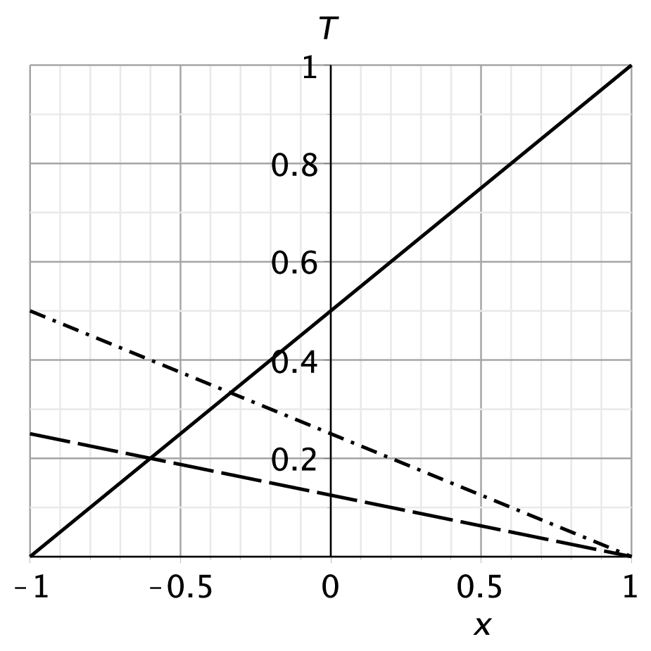
Figure 1 shows the dependence of with the initial conditions given through the parameter
| (99) |
From Eq.(50), the entanglement temperature in the diabolical point is
| (100) |
where and are respectively the maximum and minimum value of given by Eqs.(96,97,98).
Equation (100) shows that the QW initial conditions and () determine the entanglement temperature and for a fixed the isothermal lines as a function of the initial conditions are determined by the following equation
| (101) |
where is a constant.
In Fig. 2 we see that the temperature as a function of increases from for to the constant value in the interval , and then decreases gradually, reaching at . The isotherms are the intersections of the Bloch sphere with the planes .

Figure 3 shows the isotherms for the entanglement temperature as a function of the QW initial position, defined on the Bloch sphere. The figure shows three regions, two dark zones left and right, corresponding to temperatures , and the a light one corresponding to the constant temperature .
V.2 QW’s temperature for a non separable coin-position initial state I
Taking the initial state given by Eqs.(63,64) and adding Eq.(70), it is easy to show that reduces to
| (102) |
where
| (103) | |||||
| (104) |
The eigenvalues of Eq.(102) are
| (105) | |||||
| (106) | |||||
| (107) | |||||
| (108) |
The entanglement temperature Eq.(50) is thus given by
| (109) |
Figure 4 shows that the temperature as a function of increases from for , to infinity for , and then decreases gradually to at .

In order to take the initial condition on the generalized Bloch sphere, we redefine
| (110) |
| (111) |
Then the initial state Eq.(64) takes the following form
| (112) |
where and define a point on the unit Bloch sphere. In this case the isotherms have a rotation symmetry around the axis defined by the points and , North and South poles respectively. Therefore the isotherms are the parallels on the Bloch sphere. In the northern hemisphere the temperatures of the isotherms increases from , in the North pole, to infinity at the Equator, and on the southern one the temperature of the isotherms decreases from infinity at the Equator, to the finite value in the South pole.
V.3 QW’s temperature for non separable coin-position initial state II
For the 2D case, taking the initial state given by Eq.(71), after some heavy but straightforward operations, we can evaluate and they satisfy
| (113) |
which, according to Eq.(50), indicates that the temperature is infinite all over the Bloch sphere, representing a degenerate case. The symmetries of the Grover coin seem to point out that for when we use the initial condition Eq.(71).
VI Conclusion
During the last thirty years, several technological advances have made possible to construct and preserve quantum states. They also have increased the possibility of building quantum computing devices. Therefore, the study of the dynamics of open quantum systems becomes relevant both for development of these technologies as well as for the algorithms that will run on those future quantum computers. The quantum walk has emerged as a useful theoretical tool to study many fundamental aspects of quantum dynamics. It provides a frame to study, among other effects, the entanglement between its degrees of freedom, in a simple setting that often allows for a full analytical treatment of the problem. The study of this kind of entanglement is important in order to understand the asymptotic equilibrium between its internal degrees of freedom.
In this paper we have studied the asymptotic regime of the -dimensional quantum walk. We have focused into the asymptotic entanglement between chirality and position degrees of freedom, and have shown that the system establishes a stationary entanglement between the coin and the position that allows to develop a thermodynamic theory. Then we were able to generalize previous results, obtained in references [15, 37]. The asymptotic reduced density operator was used to introduce the entanglement thermodynamic functions in the canonical equilibrium. These thermodynamic functions characterize the asymptotic entanglement and the system can be seen as a particle coupled to an infinite bath, the position states. It was shown that the QW initial condition determines the system’s temperature, as well as other thermodynamic functions. A map for the isotherms was analytically built for arbitrary localized initial conditions. The behavior of the reduced density operator looks diffusive but it has a dependence on the initial conditions, the global evolution of the system being unitary. Then, if an observer only had information related with the chirality degrees of freedom, it would be very difficult for it to recognize the unitary character of the quantum evolution. In general, from this simple model we can conclude that if the quantum system dynamics occurs in a composite Hilbert space, then the behavior of the operators that acts on only one sub-space could camouflage the unitary character of the global evolution.
The development of experimental techniques has made possible the trapping of samples of atoms using resonant exchanges in momentum and energy between atoms and laser light. However, it is not yet possible to prepare a system with a particular initial chirality. Therefore, the average thermodynamical functions could have more meaning when considered from an experimental point of view. It is interesting to point out that for a given family of initial conditions, such as that given by Eq.(53), the explicit dependence of thermodynamic functions with the initial position on the Bloch’s sphere, and , can be eliminated if we take the average of over all initial conditions. Then each family could be characterized by a single asymptotic average temperature.
We acknowledge the support from PEDECIBA and ANII (FCE-2-211-1-6281, Uruguay), CNPq and LNCC (Brazil), and the CAPES-UdelaR collaboration program. FLM acknowledges financial support from FAPERJ/APQ1, CNPq/Universal and CAPES/AUXPE grants.
Appendix A
References
- [1] Y. Aharonov, L. Davidovich, and N. Zagury, Phys. Rev. A 48, 1687 (1993).
- [2] D. Aharonov, A. Ambainis, J. Kempe, and U. Vazirani. Quantum walks on graphs. In Proc. 33th STOC, pages 50–59, New York, NY, 2001.
- [3] T. D. Mackay, S. D. Bartlett, L. T. Stephenson, and B. C. Sanders. Quantum walks in higher dimensions. Journal of Physics A: Mathematical and General, 35, 2745 (2002).
- [4] B. Tregenna, W. Flanagan, R. Maile, and V. Kendon, New J. Phys. 5 83 (2003).
- [5] A.C. Oliveira, R. Portugal, and R. Donangelo. Decoherence in two-dimensional quantum walks. Phys. Rev. A, 74, 012312 (2006).
- [6] K. Watabe, N. Kobayashi, M. Katori, and N. Konno, Limit distributions of two-dimensional quantum walks, Phys. Rev. A 77, 062331 (2008).
- [7] David Aldous and James A. Fill. Reversible Markov Chains and Random Walks on Graphs. Monograph at http://www.stat.berkeley.edu/$\sim$aldous/RWG/book.html, 2002.
- [8] N. Shenvi, J. Kempe, and K.B. Whaley. A quantum random walk search algorithm. Phys. Rev. A, 67, 052307 (2003).
- [9] A. Ambainis, J. Kempe, and A. Rivosh. Coins make quantum walks faster. In Proceedings of the Sixteenth Annual ACM-SIAM Symposium on Discrete Algorithms, SODA, pages 1099–1108, 2005.
- [10] Renato Portugal. Quantum Walks and Search Algorithms. Quantum Science and Technology. Springer, New York, 2013.
- [11] E. Farhi and S. Gutmann. Quantum computation and decision trees. Phys. Rev. A, 58, 915 (1998).
- [12] A. Patel, K. S. Raghunathan, and P. Rungta. Quantum random walks do not need a coin toss. Phys. Rev. A, 71 032347 (2005).
- [13] A. Ambainis, R. Portugal, and N. Nahimovs. Spatial Search on Grids with Minimum Memory. arXiv:1312.0172, 2013.
- [14] A. Romanelli, Phys. Rev. A 81, 062349 (2010).
- [15] A. Romanelli, Phys. Rev. A 85, 012319 (2012).
- [16] W. H. Zurek, Phys. Rev. D 24 1516 (1981); Phys. Rev. D 26, 1862 (1982).
- [17] D. A. Meyer, e-print quant-ph/9804023.
- [18] Carl M. Bender and Steven A. Orszag. Advanced mathematical methods for scientists and engineers. International series in pure and applied mathematics, McGraw-Hill, New York, 1978.
- [19] M. Hinarejos, A. Pérez, Eugenio Roldán, A. Romanelli, G.J. de Valcárcel, New J. Phys. 15, 073041 (2013).
- [20] G. Grimmett, S. Janson, P.F. Scudo, Phys. Rev. E 69, 026119 (2004).
- [21] A. Nayak and A. Vishwanath, e-print quant-ph/0010117
- [22] M. Hor-Meyll, J. O. de Almeida, G. B. Lemos, P. H. Souto Ribeiro, S. P. Walborn, Phys. Rev. Letters 112, 053602 (2014).
- [23] I. Carneiro, M. Loo, X. Xu, M. Girerd, V. M. Kendon, and P. L. Knight, New J. Phys. 7, 56 (2005).
- [24] G. Abal, R. Siri, A. Romanelli, and R. Donangelo, Phys. Rev. A 73, 042302, 069905(E) (2006).
- [25] S. Salimi, R. Yosefjani, Int. J of Mod. Phys. B, 26, 1250112 (2012).
- [26] M. Annabestani, M. R. Abolhasani and, G. Abal, J.Phys. A: Math. Theor. 43, 075301 (2010).
- [27] Y. Omar, N. Paunkovic, L. Sheridan, and S. Bose, Phys. Rev. A, 74, 042304 (2006)
- [28] P. K. Pathak, and G. S. Agarwal, Phys. Rev. A, 75, 032351 (2007)
- [29] C. Liu, and N. Petulante, Phys. Rev. A 79, 032312 (2009).
- [30] S. E. Venegas-Andraca, J.L. Ball, K. Burnett, and S. Bose, New J. Phys., 7, 221 (2005).
- [31] J. Endrejat, H. Büttner, J. Phys. A: Math. Gen. 38, 9289 (2005).
- [32] A.J. Bracken, D. Ellinas, and I. Tsohantjis, J. Phys. A: Math. Gen. 37, L91 (2004).
- [33] D. Ellinas, and A.J. Bracken, Phys. Rev. A 78, 052106 (2008).
- [34] O. Maloyer, and V. Kendon, New J. Phys., 9, 87 (2007).
- [35] R. Kubo, M. Toda, and N. Hashitsume Statistical Physics II, Nonequilibrium Statistical Mechanics, Springer-Verlag, Berlin Heidelberg New York Tokyo; ISBN 3 540 11461 0, (1985).
- [36] N. Inui, Y. Konishi, and N. Konno, Phys. Rev. A Phys. Rev. E, 052323 (2004).
- [37] A. Romanelli, G. Segundo,Physica A, 393, 646 (2014).