Field Equation of Correlation Function of Mass Density Fluctuation for Self-Gravitating Systems

To understand the matter distribution in Universe on large scales is one of the major goals of modern cosmology. The large scale structure is determined by self gravity of galaxies and clusters. It brings interest to the study of self-gravitating systems. Since the number of galaxies as the typical objects is enormous, one needs statistics to study the distribution. In this regard, the $2$-point correlation function $\xi_{gg}(r)$ of galaxies and $\xi_{cc}(r)$ of clusters serve as a powerful statistical tool [11, 46]. It not only provides the statistical information, but also contains the underlying dynamics mainly due to gravitational force. Therefore, we would like to investigate the correlation functions of self gravitating system in thermal equilibrium for the first step although the real Universe is not in thermal equilibrium.

Over the years, various observational surveys have been carried out for galaxies and for clusters, such as the Automatic Plate Measuring (APM) galaxy survey [40], the Two-degree-Field Galaxy Redshift Survey (2dFGRS)[44], Sloan Digital Sky Survey (SDSS)[1], etc. All these surveys suggest that the correlation of galaxies has a power law form $\xi_{gg}(r)\propto(r_{0}/r)^{\gamma}$ with $r_{0}\sim 5.4h^{-1}$Mpc and $\gamma\sim 1.7$ in a range $(0.1\sim 10)h^{-1}$Mpc [61, 32, 46, 31, 58]. The correlation of clusters is found to be of a similar form: $\xi_{cc}(r)\sim 20\xi_{gg}(r)$ in a range $(5\sim 60)h^{-1}$Mpc, with an amplified magnitude [9, 37]. For quasars $\xi_{qq}(r)\sim 5\xi_{gg}(r)$[57].

In the past, numerical computations and simulations have been extensively employed to study the clustering of galaxies and of clusters, and significant progresses have been made. To understand the physical mechanism behind the clustering, analytical studies are important. In particular, Reference [54, 53, 52, 51] used macroscopic thermodynamic variables, such as internal energy, entropy, pressure, etc, for adequate descriptions, whereby the power-law form of $\xi_{gg}(r)$ was introduced as modifications to the energy and pressure. Similarly, Reference [22, 20] used the grand partition function of the self-gravitating gas to study a possible fractal structure of the correlation function of galaxies. However the field equation of $\xi$ was not given in these studies.

Also adopting statistical mechanics, we employ the techniques of the generating functional $Z[J]$. This practice has been well known in particle physics and condensed matter physics. The key point is that we express $Z[J]$ as a path integral over the mass density field $\psi$, instead of the gravitational potential. The functional derivatives of $\ln Z[J]$ give the connected Green functions $G^{(n)}(r_{1},...,r_{n})=\langle\delta\psi(r_{1})...\delta\psi(r_{n})\rangle$, i.e., the correlation functions of the density fluctuation $\delta\psi$ about the mean density $\psi_{0}=\langle\psi\rangle$ [67, 66]. In order to set up the field equation of the $2$-pt correlation function $G^{(2)}(r)$, we first derive the field equation of the mass density field $\psi$, which is equivalent to the well-known Lane-Emden equation for the gravitational field [28]. The use of the density field $\psi$ suits our purpose. This has been achieved by modeling the system either as a gas in thermal equilibrium, or as a fluid at rest in the gravitational field in hydrostatical equilibrium. The equation of $\psi$ is highly nonlinear. To deal with this issue, we apply the perturbation method, let $\psi=\psi_{0}+\delta\psi$, and expand the equation in terms of small quantity $\delta\psi$. We keep only up to $(\delta\psi)^{2}$ and drop off higher order terms. By taking the ensemble average of the field equation of $\psi(\bf r)$, and taking functional derivative $\delta/\delta J(\bf r)$ of the averaged equation, the field equation of $G^{(2)}(r)$ is derived. The advantage of this formulation is that the field equation of $G^{(n)}(r_{1},...,r_{n})$ for any $n$ can be also derived systematically. As is anticipated, the 3-point correlation function $G^{(3)}$ also appear in the field equation of $G^{(2)}$ to this order of perturbations. To cut off the hierarchy, $G^{(3)}$ can be expressed as the products of $G^{(2)}$ by the Kirkwood-Groth-Peebles ansatz [36, 32]. In the procedure, the quantities like $G^{(2)}(0)$, $\nabla G^{(2)}(0)$, and $\nabla^{2}G^{(2)}(0)$ also show up, as always happens for any interacting field theory when going to high orders of perturbations. After necessary renormalization to absorb these quantities, we end up with the nonlinear field equation of $G^{(2)}(r)$, also denoted as $\xi(r)$, with three parameters, $a$, $b$, $c$, as the coefficients of nonlinear terms beyond the Gaussian approximation.

The formulation applies to the system of galaxies and to the system of clusters as well, whereby the particle mass $m$ and the Jeans wavelength $\lambda_{J}$ can vary in the field equation. With a set of fixed values of $a$, $b$, $c$, the solution $\xi(r)$ will confront simultaneously the observational data of galaxies and of clusters. For galaxies, this will also be done for the power spectrum, the projected, and angular correlation functions. This work surpasses the previous sketched work [67, 66] by presenting the detailed derivation of the field equation, the renormalization, and modifications of new nonlinear terms. Besides, this work also presents the projected, and angular correlation functions, and their direct comparisons with the observations.

In section 2, we shall derive the field equation of $\psi(\bf r)$ by hydrostatics, and write down the generating functional $Z[J]$.

In section 3, we shall derive the nonlinear field equation of $\xi(r)$.

In section 4, by inspecting the resulting equation of $\xi(r)$, we shall give its several predictions about the prominent features of galaxy correlation, cluster correlation, and the large scale structure.

In section 5, we shall present the solution $\xi(r)$ for a fixed set of parameters $(a,b,c)$, and confront with the observed correlation function for galaxies. Similar comparisons will be carried out to the power spectrum, the projected, and angular correlation functions, correspondingly.

In section 6 we shall apply the same solution $\xi(r)$ with a greater mass $m$ to the system of clusters, and compare with the observational data of clusters. The observed scaling of the “correlation length” $r_{0}$ will be explained and the observed $\sim 120$Mpc periodic oscillations will be interpreted.

Section 7 contains conclusions, discusses.

In Appendix A, we give the formulation of the grand partition function of the self-gravitating system in terms of path integral over the gravitational field.

In Appendix B, by the technique of functional differentiation, we present the comprehensive details of the derivation of the field equation of $G^{(2)}(r)$ and its renormalization involved.

We use a unit with the speed of light $c=1$ and the Boltzmann constant $k_{B}=1$.

Galaxies, or clusters, distributed in Universe can be approximately described as a fluid at rest in the gravitational field due to the fluid, i.e, by hydrostatics. This modeling is an approximation since the cosmic expansion is not considered. As has been discussed by Saslaw [51], the system of galaxies in the expanding Universe is in an asymptotically relaxed state, i.e, a quasi thermal equilibrium, since the cosmic time scale $1/H_{0}$ is longer than the local crossing time scale. Therefore, the hydrostatic approximation is appropriate for a preliminary study of this paper.

In general, a fluid is described by the continuity equation, the Euler equation, and the Poisson equation :

$$\frac{\partial\rho}{\partial t}+\nabla\cdot(\rho{\bf v})=0,$$

(1)

$$\frac{\partial\bf v}{\partial t}+({\bf v}\cdot\nabla){\bf v}=-\frac{1}{\rho}\nabla p+\nabla\Phi,$$

(2)

$$\nabla^{2}\Phi=-4\pi G\rho.$$

(3)

For the hydrostatical case, $\dot{\rho}=0$ and ${\bf v}=0$, the Euler equation takes the form [38]

$$\frac{1}{\rho}\nabla p=\nabla\Phi,$$

(4)

which describes the mechanical equilibrium of the fluid. Denoting $c_{s}^{2}\equiv\partial p/\partial\rho$ with $c_{s}$ being a constant sound speed, Eq.(4) becomes

$$\frac{1}{\rho}\nabla\rho=\frac{1}{c_{s}^{2}}\nabla\Phi.$$

(5)

Taking gradient on both sides of this equation leads to

$$\nabla^{2}\rho=\frac{1}{c_{s}^{2}}(\nabla\rho\cdot\nabla\Phi+\rho\nabla^{2}\Phi).$$

(6)

Substituting Eq.(3) and (5) into the above gives

$$\nabla^{2}\rho-\frac{1}{\rho}(\nabla\rho)^{2}+\frac{4\pi G}{c_{s}^{2}}\rho^{2}=0.$$

(7)

We call Eq.(7) the field equation of mass density for the self-gravitating many-body system. For convenience, we introduce a dimensionless density field $\psi({\bf r})\equiv\rho({\bf r})/\rho_{0}$, where $\rho_{0}=mn_{0}$ is the mean mass density of the system. Then Eq.(7) takes the form

$$\nabla^{2}\psi-\frac{1}{\psi}(\nabla\psi)^{2}+k_{J}^{2}\psi^{2}=0,$$

(8)

with $k_{J}\equiv\sqrt{4\pi G\rho_{0}}/c_{s}$ being the Jeans wavenumber. This is highly nonlinear in $\psi$ as it contains $1/\psi$. Eq.(8) also follows from $\delta\mathcal{H}(\psi)/\delta\psi=0$ with the effective Hamiltonian density

$$\mathcal{H}(\psi)=\frac{1}{2}(\frac{\nabla\psi}{\psi})^{2}-k_{J}^{2}\psi.$$

(9)

To employ Schwinger’s technique of functional derivatives [56], we introduce an external source $J(\bf r)$ coupled to the field $\psi$:

$$\mathcal{H}(\psi,J)=\frac{1}{2}(\frac{\nabla\psi}{\psi})^{2}-k_{J}^{2}\psi-J\psi,$$

(10)

and the mass density field equation in the presence of $J$ is

$$\nabla^{2}\psi-\frac{1}{\psi}(\nabla\psi)^{2}+k_{J}^{2}\psi^{2}+J\psi^{2}=0.$$

(11)

This is the key equation we shall use in Section 3 to derive the field equation of correlation $G^{(2)}(r)$. The generating functional for the correlation functions of $\psi$ is defined as

$$Z[J]=\int D\psi e^{-\alpha\int d^{3}\textbf{r}\mathcal{H}(\psi,J)},$$

(12)

where $\alpha\equiv c_{s}^{2}/4\pi Gm$ with $c_{s}$ being the sound speed and $m$ being the mass of a single particle. Here $\alpha$ is introduced for proper dimension. The surveys of galaxies or clusters reveal the mass distribution, instead of the gravitational field. (We do not address a possible bias of mass distribution in this paper.) The advantage of working with the mass density field $\psi$ is to confront the observational data directly [67, 66].

Eq.(8) can also be derived from another approach. The Universe filled with galaxies and clusters can be modeled as a self gravitating gas assumed to be in thermal quasi-equilibrium [51]. Note that the Universe is expanding with a time scale $\sim 1/H_{0}=(3/8\pi G\rho_{0})^{1/2}$, and the time scale of propagation of fluctuations $\sim\lambda_{J}/c_{s}\sim 1/(4\pi G\rho_{0})^{1/2}$, both being of the same order of magnitude. The thermal equilibrium is an approximation. For such a system of $N$ particles of mass $m$, the Hamiltonian is

$$H=\sum_{i=1}^{N}\frac{p_{i}^{2}}{2m}-\sum_{i<j}^{N}\frac{Gm^{2}}{r_{ij}}$$

(13)

with $r_{ij}=|{\bf r}_{i}-{\bf r}_{j}|$, and the grand partition function is

$$Z=\sum_{N=0}^{\infty}\frac{z^{N}}{N!}\int\prod_{i=1}^{N}\frac{d^{3}p_{i}\,d^{3}r_{i}}{(2\pi)^{3}}e^{-H/T},$$

(14)

where $z$ is the fugacity. Using the Stratonovich-Hubbard transformation [59, 34], $Z$ can be converted into a path integral over a field $\phi$ [22, 68] as follows (the detailed derivation is given in Appendix A):

$$Z=\int D\phi e^{-\alpha\int d^{3}r\mathcal{H}(\phi)},$$

(15)

where the effective Hamiltonian density for $\phi$ is

$$\mathcal{H}(\phi)=\frac{1}{2}(\nabla\phi)^{2}-k_{J}^{2}e^{\phi}.$$

(16)

By $\delta\mathcal{H}(\phi)/\delta\phi=0$, Eq.(16) yields the well-known Lane-Emden equation [28, 27, 13, 2, 41]

$$\nabla^{2}\phi+k^{2}_{J}e^{\phi}=0,$$

(17)

which, by rescaling $\phi\equiv\Phi/c_{s}^{2}$, becomes the Poisson equation

$$\nabla^{2}\Phi=-4\pi G\rho(\bf r),$$

(18)

where the mass density $\rho({\bf r})=\rho_{0}e^{\Phi({\bf r})/c_{s}^{2}}$. Writing

$$\psi({\bf r})\equiv e^{\phi({\bf r})},$$

(19)

Eq.(16) and Eq.(17) become Eq.(9) and Eq.(8), respectively, as long as $\psi\neq 0$, i.e, $\phi\neq-\infty$.

Thus, for the self-gravitating system, the assumption of either thermal equilibrium, or hydrostatical equilibrium, lead to the field equation (8) of mass density, which is equivalent to the Lane-Emden equation (17). Nevertheless, Eq.(8) has the advantage that the density field $\psi$ suits better for studying the mass distribution.

In the following we outline the field equation of 2-pt correlation function, and the comprehensive details are attached in Appendix B. Since the distribution of galaxies, or clusters, can be viewed as the fluctuations of the mass density in the homogeneous Universe, we consider the fluctuation field $\delta\psi(\bf{r})\equiv\psi(\textbf{r})-\langle\psi(\textbf{r})\rangle$, where the statistical ensemble average is defined as

	$\displaystyle\langle\psi(\textbf{r})\rangle$	$\displaystyle=\frac{1}{Z}\int D\psi\,\psi e^{-\alpha\int d^{3}\textbf{r}\mathcal{H}(\psi)}$
		$\displaystyle=\frac{\delta}{\alpha\delta J({\bf r})}\log Z[J]\mid_{J=0}.$		(20)

Here the subscript $|_{J=0}$ means setting $J=0$ after taking functional derivative. $\langle\psi(\textbf{r})\rangle$ represents the mean of scaled mass density of the background, and, in our case, is a constant $\langle\psi(\textbf{r})\rangle=\psi_{0}$. The 2-point correlation function of $\delta\psi$, i.e, the connected 2-point Green function, is given by the functional derivative of $\ln Z[J]$ with respect to $J$ [10] :

	$\displaystyle G^{(2)}({\bf r}_{1},{\bf r}_{2})$	$\displaystyle\equiv\langle\delta\psi({\bf r}_{1})\delta\psi({\bf r}_{2})\rangle$
		$\displaystyle=\alpha^{-2}\frac{\delta^{2}}{\delta J({\bf r}_{1})\delta J({\bf r}_{2})}\log Z[J]|_{J=0}$
		$\displaystyle=\alpha^{-1}\frac{\delta\langle\psi({\bf r}_{2})\rangle_{J}}{\delta J({\bf r}_{1})}|_{J=0},$		(21)

where $\langle\psi(\textbf{r})\rangle_{J}\equiv\frac{\delta}{\alpha\delta J({\bf r})}\log Z[J]$ before setting $J=0$. One can take $G^{(2)}({\bf r}_{1},{\bf r}_{2})=G^{(2)}(r_{12})$ for a homogeneous and isotropic Universe. Analogously, the n-point correlation function of $\delta\psi$ is

	$\displaystyle G^{(n)}({\bf r}_{1},...,{\bf r}_{n})$	$\displaystyle\equiv\langle\delta\psi({\bf r}_{1})...\delta\psi({\bf r}_{n})\rangle$
		$\displaystyle=\alpha^{-n}\frac{\delta^{n}\log Z[J]}{\delta J({\bf r}_{1})...\delta J({\bf r}_{n})}|_{J=0}$
		$\displaystyle=\alpha^{-(n-1)}\frac{\delta^{n-1}\langle\psi({\bf r}_{n})\rangle_{J}}{\delta J({\bf r}_{1})...\delta J({\bf r}_{n-1})}|_{J=0}$		(22)

for $n\geq 3$. To derive the field equation of $G^{(2)}(r)$, as a routine [29], one takes functional derivative of the ensemble average of Eq.(11) with respect to $J({\bf r}_{1})$,

		$\displaystyle\frac{\delta}{\delta J({\bf r}_{1})}(\langle\nabla^{2}\psi({\bf r})\rangle_{J}-\langle\frac{1}{\psi({\bf r})}(\nabla\psi({\bf r}))^{2}\rangle_{J}$
		$\displaystyle+k_{J}^{2}\langle\psi({\bf r})^{2}\rangle_{J}+J({\bf r})\langle\psi({\bf r})^{2}\rangle_{J})=0,$		(23)

and then sets $J=0$. The detailed calculation is provided in Appendix B. To deal with the nonlinearity of Eq.(11) systematically, we expand it in terms of the fluctuation $\delta\psi$, and keep up to the second order $(\delta\psi)^{2}$. Then Eq.(23) leads the following equation of $G^{(2)}$:

		$\displaystyle\nabla^{2}G^{(2)}(\textbf{r})+k_{0}^{2}\psi_{0}G^{(2)}(\textbf{r})$
		$\displaystyle+[\frac{1}{2\psi_{0}^{2}}\nabla^{2}G^{(2)}(0)G^{(2)}(\textbf{r})-(\frac{1}{2\psi_{0}}\nabla^{2}+k_{J}^{2})G^{(3)}(0,{\bf r},{\bf r})$
		$\displaystyle+\frac{2}{\psi_{0}^{2}}\nabla G^{(2)}(0)\cdot\nabla G^{(2)}(\textbf{r})]=-\frac{1}{\alpha}[\psi_{0}^{2}-G^{(2)}(0)]\delta^{(3)}(\textbf{r}),$		(24)

where the characteristic wavenumber $k_{0}\equiv\sqrt{2}k_{J}$. This equation is of the same form as Eq.(4) in our previous paper [66], except that the coefficient of $G^{(3)}$ now acquires the $-k_{J}^{2}$ term, and the coefficient of the source $\delta^{(3)}(\textbf{r})$ acquires $\frac{1}{\alpha}G^{(2)}(0)$. These modifications come from an improved treatment to include high order contributions properly. Note that $G^{(3)}$ occurs in Eq.(24). There are various ways to cut off this hierarchy. In this paper, we adopt the Kirkwood-Groth-Peebles ansatz [36, 32]

	$\displaystyle G^{(3)}(\textbf{r}_{1},\textbf{r}_{2},\textbf{r}_{3})$	$\displaystyle=Q[G^{(2)}(r_{12})G^{(2)}(r_{23})+G^{(2)}(r_{23})G^{(2)}(r_{31})$
		$\displaystyle+G^{(2)}(r_{31})G^{(2)}(r_{12})],$		(25)

where $Q$ is a dimensionless parameter. This ansatz has been well-known and often used in studies of cosmology. There have been abundant data from observations and simulations as well, showing that the ansatz serves as a good fitting to the data when $Q\sim 1$. Here we take this ansatz because it gives a cutoff and has the connection to practice of cosmology. Substituting Eq.(25) into Eq.(24), after a necessary renormalization to absorb the quantities like $G^{(2)}(0)$, $\nabla G^{(2)}(0)$, and $\nabla^{2}G^{(2)}(0)$, we obtain the field equation of the 2-point correlation function

$\displaystyle(1-b\xi)\nabla^{2}\xi+k_{0}^{2}(1-c\xi)\xi+({\bf a}-b\nabla\xi)\cdot\nabla\xi=-\frac{1}{\alpha}\delta^{(3)}(\textbf{r}),$

(26)

where $\xi=\xi(r)\equiv G^{(2)}(\textbf{r})$, and $\bf a$, $b$, and $c$ are three independent parameters. The special case of ${\bf a}=b=c=0$ is the Gaussian approximation, and Eq.(26) reduces to the Helmholtz equation (B.9). Thus, the terms containing $\bf a$, $b$, and $c$ represent the nonlinear contributions beyond the Gaussian approximation. Eq.(26) in the radial direction is

$$(1-b\xi)\xi^{\prime\prime}+((1-b\xi)\frac{2}{x}+a)\xi^{\prime}+\xi-b\xi^{\prime}\,{}^{2}-c\xi^{2}=-\frac{1}{\alpha}\frac{\delta(x)k_{0}}{x^{2}},$$

(27)

where $\xi^{\prime}\equiv\frac{d}{dx}\xi$ and $x\equiv k_{0}r$. The nonlinear terms with $b$ and $c$ in Eq.(27) can enhance the amplitude of $\xi$ at small scales and increase the correlation length. The term containing $a$ plays the role of effective viscosity, and a greater $a$ leads a strong damping to the oscillations of $\xi$ at large scales, as shown in Fig.1.

The solution $\xi(r)$ will confront the observational data of galaxies and clusters in the following.

Before studying its solution, we inspect the field equation (26) to see its predictions about the general properties of the correlation function $\xi(r)$.

1, The equation contains the point mass $m$ and the characteristic wavenumber $k_{0}$. It applies to the system of galaxies, as well as to the system of clusters, with different respective $m$ and $k_{0}$ in each case. Thus, as solutions of Eq.(26), $\xi_{gg}$ for galaxies should have a profile similar to $\xi_{cc}$ for clusters, but will differ in amplitude and in scale determined by different $m$ and $k_{0}$. Indeed, the observations tell that both $\xi_{gg}$ and $\xi_{cc}$ have a power-law form: $\propto r^{-1.8}$ in their respective, finite range, but $\xi_{cc}$ has a higher amplitude[9, 37].

2, The $\delta^{3}(\bf r)$ source in Eq.(26) has the coefficient $1/\alpha=4\pi Gm/c_{s}^{2}$, which determines the overall amplitude of a solution $\xi$. The mass $m$ of a cluster can be $10\sim 10^{3}$ times that of a galaxy[4]. As for the sound speed, $c_{s}$ can be regarded as the the peculiar velocity, which is the same order of magnitude for galaxies and clusters, around several hundreds km/s [33, 42]. Therefore, $1/\alpha$ is essentially determined by $m$, and a greater $m$ will yield a higher amplitude of $\xi$. This property is clearer in the Gaussian approximation, where

$$\xi(r)\propto m$$

(28)

as revealed by the analytical solution $\xi(r)$ seen in Eq.(B.10). This general prediction naturally explains a whole chain of prominent facts of observations: luminous galaxies are more massive and have a higher correlation amplitude than ordinary galaxies [65], clusters are much more massive and have a much higher correlation than galaxies, and rich clusters have a higher correlation than poor clusters since the richness $\propto$ the mass [9, 24, 23, 3]. This phenomenon has been a puzzle for long [4] and was interpreted as being caused by the statistics of rare peak events [35].

3, The power spectrum, as the Fourier transform of $\xi(r)$, is proportional to the inverse of the spatial number density:

$$P(k)\propto 1/n_{0}.$$

(29)

See in the analytical $P(k)$ in Eq.(B.13) in the Gaussian approximation. In fact, given the mean mass density $\rho_{0}=mn_{0}$, a greater $m$ implies a lower $n_{0}$. Therefore, the properties (29) and (28) reflect the same physical law of clustering from different perspectives. The property (29) also agrees with the observational fact from a variety of surveys. The observed $P(k)$ of clusters is much higher than that of galaxies, and the observed $P(k)$ of rich clusters is higher than poor clusters, etc. This is explained by Eq.(29), since $n_{0}$ of clusters is much lower than that of galaxies, and $n_{0}$ of rich clusters is lower than that of poor clusters [5, 4].

4, The characteristic length $\lambda_{0}=2\pi/k_{0}=(\frac{\pi}{2})^{1/2}\frac{c_{s}}{\sqrt{G\rho_{0}}}\\ \propto\frac{c_{s}}{\sqrt{\rho_{0}}}$ appears in Eq.(26) as the only scale, which underlies the scale-related features of the solution $\xi(r)$. At a fixed $\lambda_{0}$, the solution $\xi(r)$ with a high amplitude drops to its first zero at a larger distance, leading to an apparently longer “correlation length”. If surveys could cover the whole Universe and if all the cosmic mass were in galaxies, which, in turn, were all contained in clusters, then $\rho_{0}$ would be the same for the system of galaxies and for the system of clusters. Nevertheless, actual cluster surveys extend over larger spatial volumes, including those very dilute regions. Therefore, $\rho_{0c}$ of the region covered by cluster surveys can be lower than $\rho_{0g}$ for galaxy surveys, and $\lambda_{0}$ for cluster surveys will be longer than that for galaxy surveys, whereas $c_{s}$ is roughly the same order of magnitude for galaxies and clusters. For instance, for rich clusters, the spatial number density $n_{c}\sim 10^{-5}$ clusters Mpc^-3 compared with $n_{g}\sim 10^{-2}$ galaxies Mpc^-3 for bright galaxies, lower by three orders [5]. But a rich cluster contains only $30\sim 300$ galaxies, the observed mass-to-light ratio of clusters flattens at $200\sim 300$ of the solar ratio $M/L$ [6], implying that clusters do not contain a substantial amount of additional dark matter, other than that associated with the galaxy halos and the hot intercluster medium [5]. These imply that $\rho_{0c}$ is lower than $\rho_{0g}$. Indeed, as will be seen in the next Section 5 and 6, to use one solution $\xi(r)$ to match the data of both galaxies and clusters, one has to take $k_{0}$ to be smaller for clusters, than for galaxies, so the system of clusters covered by the surveys has a longer $\lambda_{0}$ than the system of galaxies [17, 9].

Now we give the solution $\xi_{gg}(r)$ for a fixed set of parameters $(a,b,c)$, and confront with the observed correlation from major galaxy surveys. We will also convert $\xi_{gg}(r)$ into its associated power spectrum $P(k)$, the projected correlation function $w_{p}(r_{p})$, and the angular correlation function $w(\theta)$, and compare with the respective observational data, simultaneously.

1, The Correlation Function $\xi_{gg}(r)$.

We have taken $k_{0}=0.055$hMpc^-1 for the case of galaxies. For demonstration, two respective sets of the parameters are taken: $(a,b,c)=(1.2,0.003,0.1)$, and $(a,b,c)=(0.7,0.004,0.38)$. We remark that other values of $(a,b,c)$ can be also chosen to match the data. Figure 2 shows the solution $\xi_{gg}(r)$ and the observed data by the galaxy surveys of APM [43], SDSS [65], and 2dFGRS [33]. It is seen that the theoretical $\xi_{gg}(r)$ matches the observational data on the range of $r=(1\sim 50)$ h^-1Mpc. The usual power law fitting $\xi_{gg}\propto r^{-1.7}$ is valid only in an interval $(0.1\sim 10)$ h^-1Mpc. On large scales, the solution $\xi_{gg}(r)$ deviates from the power law, decreases rapidly to zero and becomes negative around $\sim 50$ h^-1Mpc. However, on small scales $r\leq 1$ h^-1Mpc, the solution $\xi_{gg}(r)$ is lower than the data, even though it has already improved the Gaussian approximation[67]. This insufficiency at $r\leq 1$ h^-1Mpc should be due to neglect of the high order nonlinear terms, like $(\delta\psi)^{3}$, in our perturbation. These terms should contribute more correlations on small scales. Notice that the scale $\sim 1$ h^-1Mpc is the size of a typical cluster, and the high amplitude of the observed $\xi_{gg}$ at $r\leq 1$ h^-1Mpc may come partially from the local structure of virialized clusters.

2, The Power Spectrum $P(k)$.

The power spectrum $P(k)$ is the Fourier transform

$$P(k)=4\pi\int\limits_{0}^{\infty}\xi(r)\frac{\sin(kr)}{kr}r^{2}dr$$

(30)

of the correlation function $\xi(r)$, measuring the matter density fluctuation in the $k$-space. In principle, $P(k)$ and $\xi(r)$ contain the same information if both are complete on their respective space, $k=(0,\infty)$, and $r=(0,\infty)$. Actually, the observed $\xi_{gg}(r)$ is not complete, and is actually limited to a finite range, say $r\leq 50$ Mpc. If the observed power-law $\xi_{gg}(r)=(r_{0}/r)^{1.8}$ were plugged in Eq.(30), one would have $P(k)\propto k^{-1.2}$, which does not comply with the observed $P(k)\propto k^{-1.6}$ [45]. Our solution $\xi_{gg}(r)$ is given on the whole range $r=(0,\infty)$, so it will yield a reliable $P(k)$. Figure 3 shows the theoretical $P(k)$ converted by Eq.(30) from the solution $\xi_{gg}(r)$ with the same set $(a,b,c)$ and $k_{0}$ as those in Fig.2. Also shown are the observational data of $P(k)$ from APM [43], 2dFGRS [16], and SDSS [12]. It is seen that the theoretical $P(k)$ agrees well with the data $P(k)\propto k^{-1.6}$ in the range of $k=(0.04\sim 0.7)$ hMpc^-1. However, at large $k$, the theoretical $P(k)$ is lower than the data. This insufficiency of $P(k)$ corresponds that of $\xi_{gg}(r)$ at small scales $r\leq 1$Mpc shown in Figure 2 . If high order terms like $(\delta\psi)^{3}$ are included, the theoretical $P(k)$ is expected to improve at large $k$.

3, The Projected Correlation Function $W_{p}(r_{p})$.

For actual sky surveys of galaxies and clusters, the measurement of distances is through their cosmic red-shift $z$. The galaxies or clusters have peculiar velocities, causing the red-shift distortion to the measured distance. To eliminate this distorting effect, one can make use of the unaffected part of the correlation function by integrating over the distance parallel to the line of sight. This leads to the projected correlation function [47, 46]

$\displaystyle W_{p}(r_{p})$

$\displaystyle=2\int\limits_{0}^{\infty}\xi(\sqrt{r_{p}^{2}+y^{2}})dy=2\int\limits_{r_{p}}^{\infty}\xi(r)\frac{rdr}{\sqrt{r^{2}-r_{p}^{2}}}\,,$

(31)

where $r_{p}$ is the separation of two points vertical to the line of sight, not distorted by the peculiar velocities. Figure 4 shows the theoretical $W_{p}(r_{p})$ from the solution $\xi_{gg}$ with the same $(a,b,c)$, and $k_{0}$ as those in Fig.2. The observational data from 2dFGRS [33] and SDSS [65] are also plotted for comparison. Overall, the theoretical $W_{p}(r_{p})$ traces the observational data well in the range $r_{p}=(0.6\sim 30)$h^-1Mpc, but, is lower than the data on small scales $r_{p}\leq 0.6$h^-1Mpc, the same insufficiency mentioned before.

4, The Angular Correlation Function $w(\theta)$.

To avoid the uncertainty of the distance measurements, similar to the projected $W_{p}(r_{p})$, the 2-point angular correlation function $w(\theta)$ is also used to represent the correlation between two angle positions. It also involves an integration of $\xi(r)$ along the line of sight. Specifically, fixing the azimuth angle and leaving only the altitude $\theta$, under the small separation approximation, the angular correlation function $w(\theta)$ can be derived from $\xi(r)$ by Limber’s equation [39, 50, 46]

$$w(\theta)=\int\limits_{0}^{\infty}y^{4}\phi(y)^{2}dy\int\limits_{-\infty}^{\infty}\xi(\sqrt{x^{2}+\theta^{2}y^{2}})dx,$$

(32)

where $\phi$ is the selection function, representing the combined effect of luminosity function and observer function. With the normalization $\int\limits_{0}^{\infty}\phi y^{2}dy=1$, it is given by [45]

$$\phi(y)=\frac{2}{\Gamma(\frac{5}{4})}D_{\ast}^{-\frac{5}{2}}y^{-\frac{1}{2}}e^{-(\frac{y}{D_{\ast}})^{2}},$$

(33)

where $D_{\ast}$ is the characteristic sample depth. In practice, $w(\theta)$ is given by the following integration over the wavenumber $k$ [45]

$w(\theta)=\frac{\pi}{2\Gamma^{2}(\frac{5}{4})D_{\ast}}\int\limits_{0}^{\infty}\Delta^{2}(k)\frac{dk}{k^{2}}(1-\frac{(kD_{\ast}\theta)^{2}}{8})\exp(-\frac{(kD_{\ast}\theta)^{2}}{8}),$

(34)

where $\Delta^{2}(k)\equiv k^{3}P(k)/2\pi^{2}$ and $P(k)$ is the power spectrum. Fig. 5 shows the calculated $w(\theta)$ by Eq.(34) with $P(k)$ from Fig. 3. It is seen that the theoretical curves trace the observed data well for $\theta=(0.1\sim 8)$ degree. Also, the theoretical curve is lower than the data points for $\theta\leq 0.1$ degree. For a correlation length $\lambda$, the ratio $D_{\ast}/\lambda$ measures that how much farther the survey goes beyond the correlated scale. We take $\lambda=\pi/k_{0}$ for concreteness. The survey depth of AA$\Omega$ is larger than that of SDSS [55]. Indeed, as shown in Fig. 5, to fit the data, a larger $D_{\ast}/\lambda$ for AA$\Omega$ is required than that for SDSS.

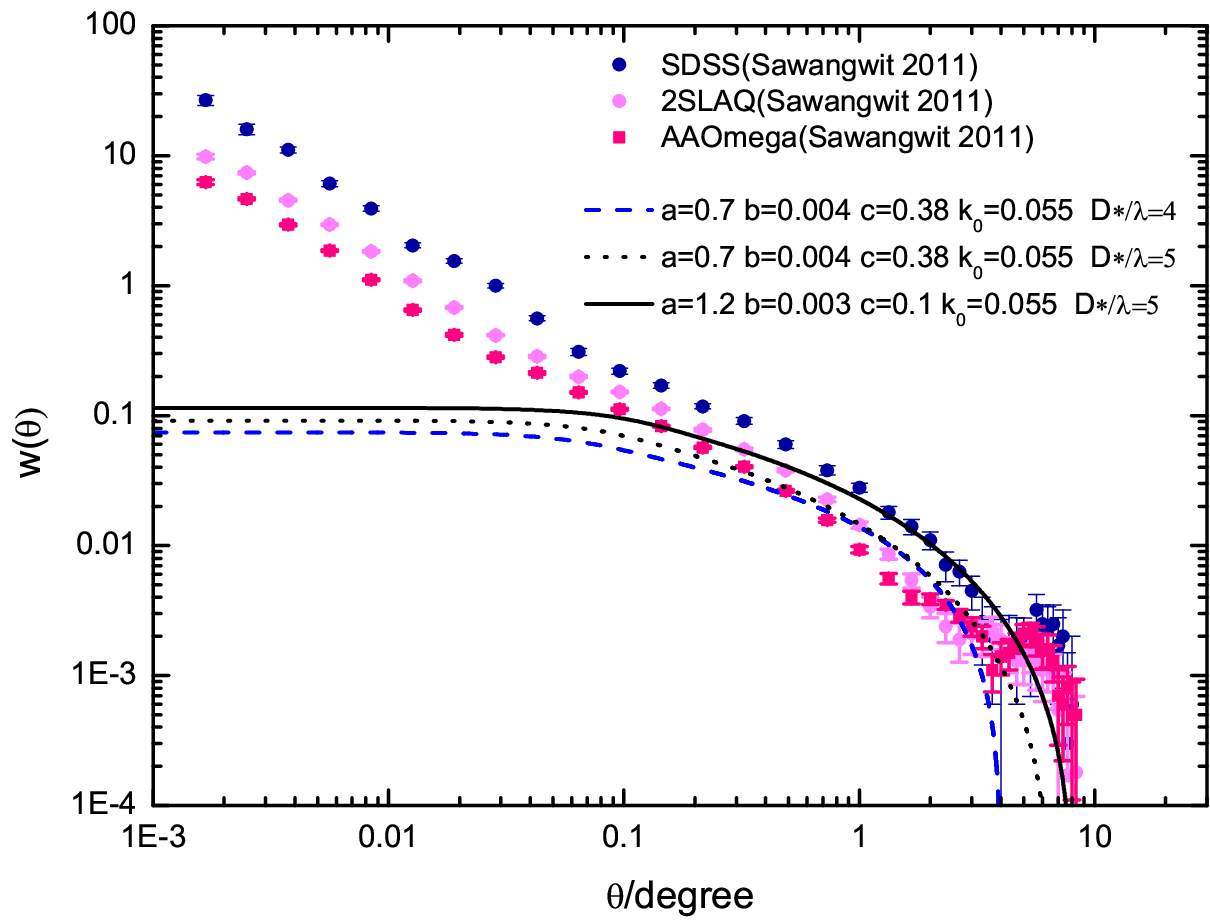
So far, with the fixed $(a,b,c)$ and $k_{0}$, the solution $\xi_{gg}(r)$ and the associated $P(k)$, $W_{p}(r_{p})$, and $w(\theta)$ simultaneously agree with the data, respectively, except the insufficiency at the small scales.

For galaxies discussed above, the observed correlation function is limited to $r\leq 50$h^-1Mpc. Clusters are believed to trace the cosmic mass distribution on even larger scales, and the observational data cover spatial scales farther than that of galaxies. Now we are going to apply the solution with the same two sets of $(a,b,c)$ as in Section 5 to the system of clusters, each being regarded as a point mass. The mass $m$ of a cluster is greater than that of a galaxy. This leads to a higher overall amplitude of $\xi_{cc}(r)$, i.e, a higher value of the boundary condition $\xi_{cc}(r_{b})$ at some point $r=r_{b}$. Besides, to match the observational data of clusters, a small value $k_{0}=0.03$ Mpc^-1 is required, smaller than the previous $k_{0}=0.055$Mpc^-1 for galaxies.

In Figure 6, for each set $(a,b,c)$ , two solutions $\xi_{cc}(r)$ with different amplitudes are given to compare with two sets of data with richness $N>10$ and $N>20$ from the SDSS [3]. To match the data of clusters of $N>20$, we have chosen a greater boundary condition $\xi(r_{b})$ than that of $N>10$, while $k_{0}$ is the same. This results in a higher correlation amplitude and an apparently longer “correlation length” for the $N>20$ clusters. Interpreted by the field equation, Eq.(26), the $N>20$ clusters have a greater $m$ than the $N>10$ clusters. The solutions match the data available on the whole range $r=(4\sim 100)$h^-1Mpc, and there is no small-scale insufficiency of correlation that occurred for the galaxy case. This indicates that, to account for the correlation of clusters, the order of $(\delta\psi)^{2}$ is accurate enough in the perturbation treatment of our formulation. Since $k_{0}=0.03$ Mpc^-1 for clusters and $k_{0}=0.055$ Mpc^-1 for galaxies, it can be inferred that the mean density $\rho_{0}$ involved in this cluster survey should be lower by $(0.03/0.055)^{2}\sim 0.3$ than those in the galaxy case.

It has long been known that, there is a scaling behavior, that is, the cluster correlation scale increases with the mean spatial separation between clusters [60, 7, 4, 18, 30]. For a power-law $\xi_{cc}=(r_{0}/r)^{1.8}$ fitting, the data indicates a “correlation length”

$$r_{0}\simeq 0.4d_{i},$$

(35)

where $d_{i}=n_{i}^{-1/3}$ and $n_{i}$ is the mean number density of clusters of type $i$. For SDSS, the scaling can be also fitted by $r_{0}\simeq 2.6d_{i}\,^{1/2}$ [3], and for the 2df galaxy groups $r_{0}\simeq 4.7d_{i}\,^{0.32}$[64]. From these surveys, the common pattern is that $r_{0}$ increases with $d_{i}$. This kind of $r_{0}-d_{i}$ scaling has been a theoretical challenge [4], and was thought to be caused by a fractal distribution of galaxies and clusters [60]. In our theory the scaling is fully embodied in the solution $\xi_{cc}(k_{0}r)$ with the characteristic wavenumber $k_{0}=(8\pi Gmn/c_{s}^{2})^{1/2}\propto d^{-3/2}$. To comply with the empirical power-law, we take the theoretical “correlation length” as $r_{0}(d)\propto\xi_{cc}^{1/1.8}$, where $\xi_{cc}$ is the theoretical solution and depends on $d$. Fig.7 shows that the solution $\xi_{cc}$ with $k_{0}=0.03$ hMpc^-1 gives the scaling $r_{0}(d)\simeq 0.4d$, agreeing well with the observation [4]. If a greater $k_{0}=0.055$ hMpc^-1 is taken, the solution $\xi_{cc}$ would yield a flatter scaling $r_{0}(d)\simeq 0.3d$, which seems to fit the data of APM clusters better[3]. This comparison tells that a higher background density $\rho_{0}$ corresponds to a flatter slope of the scaling $r_{0}(d)$. Thus the $r_{0}-d_{i}$ scaling is naturally interpreted by the solution $\xi_{cc}(k_{0}r)$.

Extended to very large scales, the observed $\xi_{cc}(r)$ exhibits a pattern of periodic oscillations with a characteristic wavelength $\sim 120$Mpc[26, 25]. This behavior was originally found in the galaxy distribution in narrow pencil beam surveys [14], also occurred in the correlation function of galaxies [62], and of quasars [63]. There have been also various interpretations on this periodic oscillations, and one is that these correspond to the superclusters of the comparable size [8]. In Figure 8, the theoretical $\xi(r)$ with small values $(a,b,c)$ exhibits periodic oscillations, which is close to the Gaussian solution [67]. To achieve the characteristic wavelength $\lambda_{0}=2\pi/k_{0}\sim 120$Mpc, one needs $k_{0}\simeq 0.053$ Mpc^-1. To yield high oscillations, a small $a=0.1$ is taken for demonstration. The data of the Abell X-ray clusters is also plotted [24], exhibiting the prominent, periodic oscillations. Qualitatively, the solution $\xi(r)$ agrees with the pattern of oscillation of the data, but has a damped amplitude at increasing $r$. The power spectrum $P(k)$ converted from the solution $\xi(r)$ with $a=0.1$ does have a prominent peak, as in Fig. 9 [25, 23]. Thus in our theory this kind of oscillations originates from the field equation itself with a sufficiently small viscosity.

We have presented a field theory of density fluctuations of a Newtonian gravitating system, applied it to the study of the correlation functions of galaxies and of clusters in a homogeneous, isotropic Universe.

As the key setup, we have obtained the field equation (8) of the mass density field $\psi$, under the condition of thermal equilibrium or hydrostatic equilibrium. It suits the studying of the mass distribution of Universe. This approach is different from those using the gravitational potential. In dealing with the high nonlinearity, we have written the field as $\psi=\psi_{0}+\delta\psi$, the order $(\delta\psi)^{2}$ has been kept in perturbations. The generating functional $Z[J]$ of the correlation functions has been written down as an path integral over $\psi$. The field equation (26) of $\xi=\langle\delta\psi\delta\psi\rangle$ has been derived as the main result, whereby the Kirkwood-Groth-Peebles ansatz and renormalization have been used. The equation is Helmholtz-like and nonlinear, with three parameters $(a,b,c)$ representing the nonlinear effects beyond the Gaussian approximation. Notably, the characteristic wavelength $\lambda_{0}$ occurs as the only scale, and the mass $m$ appears in the source. By the dependence on $m$ and $\lambda_{0}$, the equation simultaneously explains several longstanding, seemingly unrelated features of the clustering, such as the profile similarity of $\xi_{cc}$ of clusters to $\xi_{gg}$ of galaxies, the differences in amplitude and in correlation length of $\xi_{cc}$ and $\xi_{gg}$, the scaling behavior $r_{0}\simeq 0.4d$, and the pattern of periodic oscillations in $\xi_{cc}$ with a wavelength $\lambda_{0}\sim 120$Mpc.

The solution $\xi_{gg}$ for fixed $(a,b,c)$ agrees with the observational data of the galaxy surveys over a range $r=(1\sim 50)$Mpc. So do the associated power spectrum, projected correlation, and angular correlation. With the same set of $(a,b,c)$, but with a greater $m$ and a longer $\lambda_{0}$, the solution $\xi_{cc}$ also matches the data of clusters over a range $r=(4\sim 100)$h^-1Mpc. Thus, our theory sheds light on the understanding of the clustering and the large scale structure of Universe.

There are several issues and possible extensions of the current theory.

1, As is seen, the amplitude of theoretical $\xi_{gg}$ at $r\leq 1$ Mpc is lower than the observational data of galaxies. This may indicate that the actual clustering of galaxies requires higher order terms of the fluctuation beyond $(\delta\psi)^{2}$. To include $(\delta\psi)^{3}$ and the higher, the treatment will become more involved and the occurrence of $G^{(4)}$, in addition to $G^{(3)}$, will be anticipated in the field equation of $\xi_{gg}$. This extension will be our future work.

References

- [1] Abazajian K. N., Adelman-McCarthy J. K., Agüeros M. A., et al. 2009, ApJS, 182, 543
- [2] Antonov V. A., 1962, Vest. Leningrad Univ., 7, 135
- [3] Bahcall N. A., Dong F., Hao L., et al. 2003, ApJ, 599, 814
- [4] Bahcall N.A., 1999, “Clusters and Supercluster”, in Formation of Structure in the Universe, ed. by A. Dekel and J.P. Ostriker, Cambridge University Press. arXiv: astro-ph/9611148.
- [5] Bahcall N. A., 1996, arXiv:astro-ph/9611148
- [6] Bahcall N.A., Lubin L.M., Dorman V., 1995, ApJ, 447, L81
- [7] Bahcall N.A., West M., 1992, ApJL, 392, 419
- [8] Bahcall N. A., 1991, ApJ, 376, 43
- [9] Bahcall N. A., Soneira R. M. 1983, ApJ, 270, 20
- [10] Binney J., Dowrick N., Fisher A., Newman M., 1992, The Theory of Critical Phenomena, Oxford University Press
- [11] Bok B.J., 1934, Bull Harvars Obs, 895, 1
- [12] Blanton M., Tegmark M., Strauss M., 2004, ApJ, 606, 702
- [13] Bonnor W. B., 1956, MNRAS, 116, 351
- [14] Broadhurst T.J. , Ellis R. , Koo D., Szalay A., 1990, Nat, 343, 34
- [15] Chandrasekhar S., 1939, An introduction to the Study of Stellar Structure. Chicago Univ. Press
- [16] Cole S., Percival W. J., Peacock J. A., et al., 2005, MNRAS, 362, 505
- [17] Collins C. A., Guzzo L., Böhringer H., et al., 2000, MNRAS, 319, 939
- [18] Croft R. A. C., Dalton G. B., Efstathiou G., Sutherland W. J., Maddox S. J., 1997, MNRAS, 291, 305
- [19] Davis M., Peebles P.J.E., 1983, ApJ, 267, 465
- [20] de Vega, H.J., Sanchez, N., Combes, F., 1998, ApJ, 500, 8
- [21] de Vega, H.J., Sanchez, N., Combes, F., 1996, Phys.Rev. D, 54, 6008
- [22] de Vega H.J., Sanchez N., Combes F., 1996, Nature, 383, 56
- [23] Einasto M., Einasto J., Tago E., et al., 2007, ApJ, 123, 51. arXiv:astro-phy/0012538
- [24] Einasto M., Einasto J., Tago E., Andernach H., Dalton G. B., Müller V., 2002, AJ, 123, 51
- [25] Einasto J., Einasto M., Gottloeber S., et al., 1997, Nature, 385, 139
- [26] Einasto J., Einasto M., Frisch P., et al., 1997, MNRAS, 289, 801
- [27] Ebert R., 1955, Z. Astrophys., 37, 217
- [28] Emden R., 1907, Gaskugeln, Leipzig and Berlin
- [29] Goldenfeld N., 1992, Lectures on Phase Transitions and Renormalization Group, Addison-Wesley Publishing Company
- [30] Gonzalez A. H., Zaritsky D., Wechler R. H., 2002, ApJ, 571, 129
- [31] Groth E., Peebles P.J.E., 1986, ApJ , 310, 507
- [32] Groth E., Peebles P.J.E., 1977, ApJ, 217, 385
- [33] Hawkins E., Maddox S., Cole S., et al., 2003, MNRAS, 346, 78
- [34] Hubbard, J., 1959, Phys. Rev. Lett., 3, 77
- [35] Kaiser N., 1984, ApJ, 284, L9
- [36] Kirkwood J.G. 1932, J. Chem. Phys., 3, 300
- [37] Klypin A.A., Kopylov A.I., 1983, Sov. Astron. Lett. ,9, 41.
- [38] Landau L.D., Lifshitz E.M., 1987, Fluid Mechanics, Pergamon Press
- [39] Limber D. N., 1953, ApJ, 117, 134
- [40] Loveday J., Peterson B.A., Maddox S.J., Efstathiou G., 1996, ApJS, 107, 201
- [41] Lynden-Bell D., Wood R., 1968, MNRAS, 138, 495
- [42] Masters K. L., Springob C. M., Haynes M. P., Giovanelli R., 2006, ApJ, 653, 861
- [43] Padilla N.D., Baugh C.M., 2003, MNRAS, 343, 796
- [44] Peacock J., Cole S., Norberg P., et al., 2001, Nature, 410, 169
- [45] Peacock J. A., 1999, Cosmological Physics. Cambridge Univ. Press, Cambridge, UK
- [46] Peebles P. J. E., 1980,The Large-scale Structure of the Universe. Princeton Univ. Press, Princeton, NJ
- [47] Peebles P.J.E., 1976, Ap. Space Sci. , 45, 3
- [48] Peebles P.J.E., 1974, ApJ, 189, L51
- [49] Peebles P.J.E., 1974, A&A, 32, 197
- [50] Rubin V.C., 1954, Proc. N.A.S, 40, 541
- [51] Saslaw W.C., 2000, The Distribution of the Galaxies. Cambridge University Press.
- [52] Saslaw W.C., 1985, Gravitational Physics of Steller and Galactic Systems. Cambridge University Press.
- [53] Saslaw W.C., 1969, MNRAS ,143 ,437
- [54] Saslaw W.C., 1968, MNRAS ,141, 1
- [55] Sawangwit U., Shanks T., Abdalla F. B., et al., 2011, MNRAS, 416, 3033
- [56] Schwinger J., 1951, Proc. Natl. Acamd. Sci. USA ,37, 452, 455.
- [57] Shaver P., 1988, in Large-Scale Structure of the Universe, IAU Symp. 130, ed. J. Audouze et al. ,Dordrecht: Reidel, 359
- [58] Soneira R.M., Peebles P.J.E. 1987, AJ , 83, 845
- [59] Stratonovich R.L., 1958, Doklady, 2, 146
- [60] Szalay A., Schramm D., 1985, Nature, 314, 718.
- [61] Totsuji H., Kihara T., 1969, PASJ, 21, 221
- [62] Tucker D. L., Oemler A., Jr., Kirshner R. P., et al., 1997, MNRAS, 285, L5
- [63] Yahata K., Suto Y., Kayo I., et al., PASJ, 57, 529
- [64] Zandivarez A., Merchan M. E., Padilla N. D., 2003, MNRAS, 344, 247
- [65] Zehavi I., Zheng Z., Weinberg D. H., et al. 2005, ApJ, 630, 1
- [66] Zhang Y., Miao H. X., 2009, Research in Astron. and Astrophys., 9, 501
- [67] Zhang Y., 2007, A&A, 464, 811
- [68] Zinn-Justin J., 1996, Quantum Field Theory and Critical Phenomena. Oxford Univ. Press, Oxford
Appendix A Stratonovich-Hubbard Transformation and Grand Partition Function as a Path Integral
From the identity