跳到论文正文
W Papers独立论文阅读器 arXiv:1408.5119 论文正文 计算阅读时间 · 0%
引用这篇论文根据当前论文元数据生成,正式投稿前建议核对。


License: arXiv.org perpetual non-exclusive license
arXiv:1408.5119v3 [math.OC] 14 Jan 2015

Polynomial optimization with applications to stability analysis and Control - Alternatives to Sum of SquaresThanks: Acknowledgements: NSF grant No. CMMI-1151018 and CMMI-1100376

Abstract.

In this paper, we explore the merits of various algorithms for polynomial optimization problems, focusing on alternatives to sum of squares programming. While we refer to advantages and disadvantages of Quantifier Elimination, Reformulation Linear Techniques, Blossoming and Groebner basis methods, our main focus is on algorithms defined by Polya’s theorem, Bernstein’s theorem and Handelman’s theorem. We first formulate polynomial optimization problems as verifying the feasibility of semi-algebraic sets. Then, we discuss how Polya’s algorithm, Bernstein’s algorithm and Handelman’s algorithm reduce the intractable problem of feasibility of semi-algebraic sets to linear and/or semi-definite programming. We apply these algorithms to different problems in robust stability analysis and stability of nonlinear dynamical systems. As one contribution of this paper, we apply Polya’s algorithm to the problem of H∞H_{\infty} control of systems with parametric uncertainty. Numerical examples are provided to compare the accuracy of these algorithms with other polynomial optimization algorithms in the literature.

Key words and phrases: 
Polynomial optimization, Polya’s theorem, Handelman’s theorem, Lyapunov stability analysis, Convex optimization
1991 Mathematics Subject Classification
Primary: 93D05, 93D09; Secondary: 90C22.

Reza Kamyar

School of Matter, Transport and Energy

Arizona State University

Goldwater Center for Science and Engineering 531

Tempe, 85281, USA

Matthew M. Peet

School of Matter, Transport and Energy

Arizona State University

501 Tyler Mall - ECG 301

Tempe, 85281, USA

1. Introduction

Consider problems such as portfolio optimization, structural design, local stability of nonlinear ordinary differential equations, control of time-delay systems and control of systems with uncertainties. These problems can all be formulated as polynomial optimization or optimization of polynomials. In this paper, we survey how computation can be applied to polynomial optimization and optimization of polynomials. One example of polynomial optimization is β∗=minx∈ℝn⁡p⁡(x)\beta^{*}=\min_{x\in\mathbb{R}^{n}}p(x), where p:ℝn→ℝp:\mathbb{R}^{n}\rightarrow\mathbb{R} is a multi-variate polynomial. In general, since p⁡(x)p(x) is not convex, this is not a convex optimization problem. It is well-known that polynomial optimization is NP-hard [1]. We refer to the dual problem to polynomial optimization as optimization of polynomials, e.g., the dual optimization of polynomials to β∗=minx∈ℝn⁡p⁡(x)\beta^{*}=\min_{x\in\mathbb{R}^{n}}p(x) is

β∗=maxy∈ℝ⁡y\displaystyle\quad\beta^{*}=\max_{y\in\mathbb{R}}\;y
subject to ​p​(x)−y≥0​ for all ​x∈ℝn.\displaystyle\text{subject to }\;\;p(x)-y\geq 0\text{ for all }x\in\mathbb{R}^{n}. (1)

This problem is convex, yet NP-hard.

One approach to find lower bounds on the optimal objective β∗\beta^{*} is to apply Sum of Squares (SOS) programming [7, 8]. A polynomial pp is SOS if there exist polynomials qiq_{i} such that p⁡(x)=∑i=1rqi​(x)2p(x)=\sum_{i=1}^{r}q_{i}(x)^{2}. The set {qi∈ℝ⁡[x],i=1,⋯,r}\{q_{i}\in\mathbb{R}[x],i=1,\cdots,r\} is called an SOS decomposition of p⁡(x)p(x), where ℝ⁡[x]\mathbb{R}[x] is the ring of real polynomials. An SOS program is an optimization problem of the form

minx∈ℝmcT​x\displaystyle\quad\min_{x\in\mathbb{R}^{m}}\qquad c^{T}x
subject toAi,0​(y)+∑j=1mxj​Ai,j​(y)​ is SOS, ​i=1,⋯,k,\displaystyle\text{subject to}\quad A_{i,0}(y)+\sum_{j=1}^{m}x_{j}A_{i,j}(y)\text{ is SOS, }i=1,\cdots,k, (2)

where c∈ℝmc\in\mathbb{R}^{m} and Ai,j∈ℝ⁡[y]A_{i,j}\in\mathbb{R}[y] are given. If p⁡(x)p(x) is SOS, then clearly p⁡(x)≥0p(x)\geq 0 on ℝn\mathbb{R}^{n}. While verifying p⁡(x)≥0p(x)\geq 0 on ℝn\mathbb{R}^{n} is NP-hard, checking whether p⁡(x)p(x) is SOS - hence non-negative - can be done in polynomial time [7]. It was first shown in [7] that verifying the existence of a SOS decomposition is a Semi-Definite Program. Fortunately, there exist several algorithms [9, 10, 11] and solvers [12, 14, 13] that solve SDPs to arbitrary precision in polynomial time. To find lower bounds on β∗=minx∈ℝn⁡p⁡(x)\beta^{*}=\min_{x\in\mathbb{R}^{n}}p(x), consider the SOS program

y∗=maxy∈ℝ⁡y​ subject to ​p​(x)−y​ is SOS.y^{*}=\max_{y\in\mathbb{R}}y\;\text{ subject to }\;p(x)-y\text{ is SOS}.

Clearly y∗≤β∗y^{*}\leq\beta^{*}. By performing a bisection search on yy and semi-definite programming to verify p⁡(x)−yp(x)-y is SOS, one can find y∗y^{*}. SOS programming can also be used to find lower bounds on the global minimum of polynomials over a semi-algebraic set S:={x∈ℝn:gi(x)≥0,hj(x)=0}S:=\{x\in\mathbb{R}^{n}:g_{i}(x)\geq 0,h_{j}(x)=0\} generated by gi,hj∈ℝ⁡[x]g_{i},h_{j}\in\mathbb{R}[x]. Given problem (1) with x∈Sx\in S, Positivstellensatz results [15, 16, 17] define a sequence of SOS programs whose objective values form a sequence of lower bounds on the global minimum β∗\beta^{*}. It is shown that under certain conditions on SS [16], the sequence of lower bounds converges to the global minimum. See [18] for a comprehensive discussion on the Positivstellensatz.

In this paper, we explore the merits of some of the alternatives to SOS programming. There exist several results in the literature that can be applied to polynomial optimization; e.g., Quantifier Elimination (QE) algorithms [19] for testing the feasibility of semi-algebraic sets, Reformulation Linear Techniques (RLTs) [20, 21] for linearizing polynomial optimizations, Polya’s result [2] for positivity on the positive orthant, Bernstein’s [22, 23] and Handelman’s [24] results for positivity on simplices and convex polytopes, and other results based on Groebner bases [3] and Blossoming [4]. We will discuss Polya’s, Bernstein’s and Handelman’s results in more depth. The discussion of the other results are beyond the scope of this paper, however the ideas behind these results can be summarized as follows.

QE algorithms apply to First-Order Logic formulae, e.g.,

∀x​∃y⁡(f⁡(x,y)≥0⇒((g⁡(a)<x​y)∧(a>2))CLOSE,\forall x\,\exists y\,(f(x,y)\geq 0\Rightarrow((g(a)<xy)\wedge(a>2)),

to eliminate the quantified variables xx and yy (preceded by quantifiers ∀,∃\forall,\exists) and construct an equivalent formula in terms of the unquantified variable aa. The key result underlying QE algorithms is Tarski-Seidenberg theorem [5]. The theorem implies that for every formula of the form ∀x∈ℝn​∃y∈ℝm​(fi​(x,y,a)≥0)\forall x\in\mathbb{R}^{n}\,\exists y\in\mathbb{R}^{m}(f_{i}(x,y,a)\geq 0), where fi∈ℝ⁡[x,y,a]f_{i}\in\mathbb{R}[x,y,a], there exists an equivalent quantifier-free formula of the form ∧i(gi(a)≥0)∨j(hj(a)≥0)\wedge_{i}(g_{i}(a)\geq 0)\vee_{j}(h_{j}(a)\geq 0) with gi,hj∈ℝ⁡[a]g_{i},h_{j}\in\mathbb{R}[a]. QE implementations [25, 26] with a bisection search yields the exact solution to optimization of polynomials, however the complexity scales double exponentially in the dimension of variables x,yx,y.

RLT was initially developed to find the convex hull of feasible solutions of zero-one linear programs [27]. It was later generalized to address polynomial optimizations of the form minx⁡p⁡(x)\min_{x}p(x) subject to x∈[0,1]n∩Sx\in[0,1]^{n}\cap S [20]. RLT constructs a δ−\delta-hierarchy of linear programs by performing two steps. In the first step (reformulation), RLT introduces the new constraints ∏ixi​∏j(1−xj)≥0\prod_{i}x_{i}\prod_{j}(1-x_{j})\geq 0 for all i,j:i+j=δi,j:i+j=\delta. In the second step (linearization), RTL defines a linear program by replacing every product of variables xix_{i} by a new variable. By increasing δ\delta and repeating the two steps, one can construct a δ−\delta-hierarchy of lower bounding linear programs. A combination of RLT and branch-and-bound partitioning of [0,1]n[0,1]^{n} was developed in [21] to achieve tighter lower bounds on the global minimum. For a survey of different extensions of RLT see [6].

Groebner bases can be used to reduce a polynomial optimization over a semi-algebraic set S:={x∈ℝn:gi(x)≥0,hj(x)=0}S:=\{x\in\mathbb{R}^{n}:g_{i}(x)\geq 0,\,h_{j}(x)=0\} to the problem of finding the roots of univariate polynomials [28]. First, one needs to construct the system of polynomial equations

∇xL(x,λ,μ),∇λL(x,λ,μ),∇μL(x,λ,μ)]=0,\nabla_{x}L(x,\lambda,\mu),\nabla_{\lambda}L(x,\lambda,\mu),\nabla_{\mu}L(x,\lambda,\mu)]=0, (3)

where L:=p⁡(x)+∑iλi​gi​(x)+∑jμj​hj​(x)L:=p(x)+\sum_{i}\lambda_{i}g_{i}(x)+\sum_{j}\mu_{j}h_{j}(x) is the Lagrangian. It is well-known that the set of solutions to (3) is the set of extrema of the polynomial optimization minx∈S⁡p⁡(x)\min_{x\in S}p(x). Let

[f1​(x,λ,μ),⋯,fN​(x,λ,μ)]:=[∇xL​(x,λ,μ),∇λL​(x,λ,μ),∇μL​(x,λ,μ)].\left[f_{1}(x,\lambda,\mu),\cdots,f_{N}(x,\lambda,\mu)\right]:=\left[\nabla_{x}L(x,\lambda,\mu),\nabla_{\lambda}L(x,\lambda,\mu),\nabla_{\mu}L(x,\lambda,\mu)\right].

Using the elimination property [3] of the Groebner bases, the minimal Groebner basis of the ideal of f1,⋯,fNf_{1},\cdots,f_{N} defines a triangular-form system of polynomial equations. This system can be solved by calculating one variable at a time and back-substituting into other polynomials. The most computationally expensive part is the calculation of the Groebner basis, which in the worst case scales double-exponentially in the number of decision variables.

The blossoming approach involves mapping the space of polynomials to the space of multi-affine functions (polynomials that are affine in each variable). By using this map and the diagonal property of blossoms [4], one can reformulate any polynomial optimization minx∈S⁡p⁡(x)\min_{x\in S}p(x) as an optimization of multi-affine functions. In [30], it is shown that the dual to optimization of multi-affine functions over a hypercube is a linear program. The optimal objective value of this linear program is a lower bound on the minimum of p⁡(x)p(x) over the hypercube.

While the discussed algorithms have advantages and disadvantages (such as exponential complexity), we focus on Polya’s, Bernstein’s and Handelman’s theorems - results which yield polynomial-time parameterizations of positive polynomials. Polya’s theorem yields a basis to parameterize the cone of polynomials that are positive on the positive orthant. Bernstein’s and Handelman’s theorems yield a basis to parameterize the space of polynomials that are positive on simplices and convex polytopes. Similar to SOS programming, one can find Polya’s, Bernstein’s and Handelman’s parameterizations by solving a sequence of Linear Programs (LPs) and/or SDPs. However, unlike the SDPs associated with SOS programming, the SDPs associated with these theorems have a block-diagonal structure. This structure has been exploited in [29] to design parallel algorithms for optimization of polynomials with large degrees and number of variables. Unfortunately, unlike SOS programming, Bernstein’s, Handelman’s and the original Polya’s theorems do not parameterize polynomials with zeros in the positive orthant. Yet, there exist some variants of Polya’s theorem which considers zeros at the corners [31] and edges [32] of simplices. Moreover, there exist other variants of Polya’s theorem which provide certificates of positivity on hypercubes [33, 34], intersection of semi-algebraic sets and the positive orthant [35] and the entire ℝn\mathbb{R}^{n} [36], or apply to polynomials with rational exponents [37].

We organize this paper as follows. In Section 2, we place Polya’s, Bernstein’s, Handelman’s and the Positivstellensatz results in the broader topic of research on polynomial positivity. In Section 3, we first define polynomial optimization and optimization of polynomials. Then, we formulate optimization of polynomials as the problem of verifying the feasibility of semi-algebraic sets. To verify the feasibility of different semi-algebraic sets, we present algorithms based on the different variants of Polya’s, Bernstein’s, Handelman’s and Positivstellensatz results. In Section 4, we discuss how these algorithms apply to robust stability analysis [38, 29, 39] and nonlinear stability [41, 42, 43, 44]. Finally, one contribution of this paper is to apply Polya’s algorithm to the problem of H∞H_{\infty} control synthesis for systems with parametric uncertainties.

2. Background on positivity of polynomials

In 1900, Hilbert published a list of mathematical problems, one of which was: For every non-negative f∈ℝ⁡[x]f\in\mathbb{R}[x], does there exist some non-zero q∈ℝ⁡[x]q\in\mathbb{R}[x] such that q2​fq^{2}f is a sum of squares? In other words, is every non-negative polynomial a sum of squares of rational functions? This question was motivated by his earlier works [48, 49], in which he proved: 1- Every non-negative bi-variate degree 4 homogeneous polynomial (A polynomial whose monomials all have the same degree) is a SOS of three polynomials. 2- Every bi-variate non-negative polynomial is a SOS of four rational functions. 3- Not every homogeneous polynomial with more than two variables and degree greater than 5 is SOS of polynomials. Eighty years later, Motzkin constructed a non-negative degree 6 polynomial with three variables which is not SOS [50]:

M⁡(x1,x2,x3)=x14​x22+x12​x24−3​x12​x22​x32+x36.M(x_{1},x_{2},x_{3})=x_{1}^{4}x_{2}^{2}+x_{1}^{2}x_{2}^{4}-3x_{1}^{2}x_{2}^{2}x_{3}^{2}+x_{3}^{6}.

Robinson [51] generalized Motzkin’s example as follows. Polynomials of the form (∏i=1nxi2)​f​(x1,⋯,xn)+1(\prod_{i=1}^{n}x_{i}^{2})f(x_{1},\cdots,x_{n})+1 are not SOS if polynomial ff of degree <2​n<2n is not SOS. Hence, although the non-homogeneous Motzkin polynomial M⁡(x1,x2,1)=x12​x22​(x12+x22−3)+1M(x_{1},x_{2},1)=x_{1}^{2}x_{2}^{2}(x_{1}^{2}+x_{2}^{2}-3)+1 is non-negative it is not SOS.

In 1927, Artin answered Hilbert’s problem in the following theorem [52].

Theorem 2.1.

(Artin’s theorem) A polynomial f∈ℝ⁡[x]f\in\mathbb{R}[x] satisfies f⁡(x)≥0f(x)\geq 0 on ℝn\mathbb{R}^{n} if and only if there exist SOS polynomials NN and D≠0D\neq 0 such that f⁡(x)=N⁡(x)D⁡(x)f(x)=\frac{N(x)}{D(x)}.

Although Artin settled Hilbert’s problem, his proof was neither constructive nor gave a characterization of the numerator NN and denominator DD. In 1939, Habicht [54] showed that if ff is positive definite and can be expressed as f⁡(x1,⋯,xn)f(x_{1},\cdots,x_{n}) =g⁡(x12,⋯,xn2)=g(x_{1}^{2},\cdots,x_{n}^{2}) for some polynomial gg, then one can choose the denominator D=∑i=1nxi2D=\sum_{i=1}^{n}x_{i}^{2}. Moreover, he showed that by using D=∑i=1nxi2D=\sum_{i=1}^{n}x_{i}^{2}, the numerator NN can be expressed as a sum of squares of monomials. Habicht used Polya’s theorem ([53], Theorem 56) to obtain the above characterizations for NN and DD.

Theorem 2.2.

(Polya’s theorem) Suppose a homogeneous polynomial pp satisfies p⁡(x)>0p(x)>0 for all x∈{x∈ℝn:xi≥0,∑i=1nxi≠0}x\in\{x\in\mathbb{R}^{n}:x_{i}\geq 0,\sum_{i=1}^{n}{x_{i}}\neq 0\}. Then p⁡(x)p(x) can be expressed as

p⁡(x)=N⁡(x)D⁡(x),p(x)=\dfrac{N(x)}{D(x)},

where N⁡(x)N(x) and D⁡(x)D(x) are homogeneous polynomials with all positive coefficients. For every homogeneous p⁡(x)p(x) and some e≥0e\geq 0, the denominator D⁡(x)D(x) can be chosen as (x1+⋯+xn)e(x_{1}+\cdots+x_{n})^{e}.

Suppose ff is homogeneous and positive on the positive orthant and can be expressed as f⁡(x1,⋯,xn)=g⁡(x12,⋯,xn2)f(x_{1},\cdots,x_{n})=g(x_{1}^{2},\cdots,x_{n}^{2}) for some homogeneous polynomial gg. By using Polya’s theorem g⁡(y)=N⁡(y)D⁡(y)g(y)=\frac{N(y)}{D(y)}, where y:=(y1,⋯,yn)y:=(y_{1},\cdots,y_{n}) and polynomials NN and DD have all positive coefficients. By Theorem 2.2 we may choose D⁡(y)=(∑i=1nyi)eD(y)=\left(\sum_{i=1}^{n}y_{i}\right)^{e}. Then (∑i=1nyi)e​g​(y)=N⁡(y)\left(\sum_{i=1}^{n}y_{i}\right)^{e}g(y)=N(y). Now let xi=yix_{i}=\sqrt{y_{i}}, then (∑i=1nxi2)e​f​(x1,⋯,xn)=N⁡(x12,⋯,xn2)\left(\sum_{i=1}^{n}x_{i}^{2}\right)^{e}f(x_{1},\cdots,x_{n})=N(x_{1}^{2},\cdots,x_{n}^{2}). Since NN has all positive coefficients, N⁡(x12,⋯,xn2)N(x_{1}^{2},\cdots,x_{n}^{2}) is a sum of squares of monomials. Unlike the case of positive definite polynomials, it is shown that there exists no single SOS polynomial D≠0D\neq 0 which satisfies f=NDf=\frac{N}{D} for every positive semi-definite ff and some SOS polynomial NN [55].

As in the case of positivity on ℝn\mathbb{R}^{n}, there has been an extensive research regarding positivity of polynomials on bounded sets. A pioneering result on local positivity is Bernstein’s theorem (1915) [56]. Bernstein’s theorem uses the polynomials hi,j=(1+x)i​(1−x)jh_{i,j}=(1+x)^{i}(1-x)^{j} as a basis to parameterize univariate polynomials which are positive on [−1,1][-1,1].

Theorem 2.3.

(Bernstein’s theorem) If a polynomial f⁡(x)>0f(x)>0 on [−1,1][-1,1], then there exist ci,j>0c_{i,j}>0 such that

f⁡(x)=∑i,j∈ℕi+j=dci,j​(1+x)i​(1−x)jf(x)=\sum_{\begin{subarray}{c}i,j\in\mathbb{N}\\ i+j=d\end{subarray}}c_{i,j}(1+x)^{i}(1-x)^{j}

for some d>0d>0.

Reference [57] uses Goursat’s transform of ff to find an upper bound on dd. The bound is a function of the minimum of ff on [−1,1][-1,1]. However, computing the minimum itself is intractable. In 1988, Handelman [58] used products of affine functions as a basis (the Handelman basis) to extend Bernstein’s theorem to multi-variate polynomials which are positive on convex polytopes.

Theorem 2.4.

(Handelman’s Theorem) Given wi∈ℝnw_{i}\in\mathbb{R}^{n} and ui∈ℝu_{i}\in\mathbb{R}, define the polytope ΓK:={x∈ℝn:wiTx+ui≥0,i=1,⋯,K}\Gamma^{K}:=\{x\in\mathbb{R}^{n}:w_{i}^{T}x+u_{i}\geq 0,i=1,\cdots,K\}. If a polynomial f⁡(x)>0f(x)>0 on ΓK\Gamma^{K}, then there exist bα≥0b_{\alpha}\geq 0, α∈ℕK\alpha\in\mathbb{N}^{K} such that for some d∈ℕd\in\mathbb{N},

f(x)=∑α∈ℕKα1+⋯+αK≤dbα(w1Tx+u1)α1⋯(wKTx+uK)αK.f(x)=\sum_{\begin{subarray}{c}\alpha\in\mathbb{N}^{K}\\ \alpha_{1}+\cdots+\alpha_{K}\leq d\end{subarray}}b_{\alpha}(w_{1}^{T}x+u_{1})^{\alpha_{1}}\cdots(w_{K}^{T}x+u_{K})^{\alpha_{K}}. (4)

In [22], first the standard triangulation of a simplex (the convex hull of vertices in ℝn\mathbb{R}^{n}) is developed to decompose an arbitrary simplex into sub-simplices. Then, an algorithm is proposed to ensure positivity of a polynomial ff on the simplex by finding an expression of Form (4) for ff on each sub-simplex. An upper bound on the degree dd in (4) was provided in [23] as a function of the minimum of ff on the simplex, the number of variables of ff, the degree of ff and the maximum of certain [23] affine combinations of the coefficients bαb_{\alpha}. Reference [22] also provides a bound on dd as a function of maxα⁡bα\max_{\alpha}b_{\alpha} and the minimum of ff over the polytope.

An extension of Handelman’s theorem was made by Schweighofer [59] to verify non-negativity of polynomials over compact semi-algebraic sets. Schweighofer used the cone of polynomials in (5) to parameterize any polynomial ff which has the following properties:

  1. (1)

    ff is non-negative over the compact semi-algebraic set SS

  2. (2)

    f=q1​p1+q2​p2+⋯f=q_{1}p_{1}+q_{2}p_{2}+\cdots for some qiq_{i} in the cone (5) and for some pi>0p_{i}>0 over S∩{x∈ℝn:f⁡(x)=0}S\cap\{x\in\mathbb{R}^{n}:f(x)=0\}

Theorem 2.5.

(Schweighofer’s theorem) Suppose

S:={x∈ℝn:gi(x)≥0,gi∈ℝ[x] for i=1,⋯,K}S:=\{x\in\mathbb{R}^{n}:g_{i}(x)\geq 0,g_{i}\in\mathbb{R}[x]\text{ for }i=1,\cdots,K\}

is compact. Define the following set of polynomials which are positive on SS.

Θd:={∑λ∈ℕK:λ1+⋯+λK≤dsλg1λ1⋯gKλK:sλ are SOS }\Theta_{d}:=\left\{\sum_{\begin{subarray}{c}\lambda\in\mathbb{N}^{K}:\lambda_{1}+\cdots+\lambda_{K}\leq d\end{subarray}}s_{\lambda}g_{1}^{\lambda_{1}}\cdots g_{K}^{\lambda_{K}}:s_{\lambda}\text{ are SOS }\right\} (5)

If f≥0f\geq 0 on SS and there exist qi∈Θdq_{i}\in\Theta_{d} and polynomials pi>0p_{i}>0 on S∩{x∈ℝn:f⁡(x)=0}S\cap\{x\in\mathbb{R}^{n}:f(x)=0\} such that f=∑iqi​pif=\sum_{i}q_{i}p_{i} for some dd, then f∈Θdf\in\Theta_{d}.

On the assumption that gig_{i} are affine functions, pi=1p_{i}=1 and sλs_{\lambda} are constant, Schweighofer’s theorem gives the same parameterization of ff as in Handelman’s theorem. Another special case of Schweighofer’s theorem is when λ∈{0,1}K\lambda\in\{0,1\}^{K}. In this case, Schweighofer’s theorem reduces to Schmudgen’s Positivstellensatz [17]. Schmudgen’s Positivstellensatz states that the cone

Λg:={∑λ∈{0,1}Ksλg1λ1⋯gKλK:sλ are SOS}⊂Θd\Lambda_{g}:=\left\{\sum_{\lambda\in\{0,1\}^{K}}s_{\lambda}g_{1}^{\lambda_{1}}\cdots g_{K}^{\lambda_{K}}:s_{\lambda}\text{ are }SOS\right\}\subset\Theta_{d} (6)

is sufficient to parameterize every f>0f>0 over the semi-algebraic set SS generated by {g1,⋯,gK}\{g_{1},\cdots,g_{K}\}. Unfortunately, the cone Λg\Lambda_{g} contains 2K2^{K} products of gig_{i}, thus finding a representation of Form (6) for ff requires a search for at most 2K2^{K} SOS polynomials. Putinar’s Positivstellensatz [16] reduces the complexity of Schmudgen’s parameterization in the case where the quadratic module of gig_{i} defined in (7) is Archimedean, i.e., for every p∈ℝ⁡[x]p\in\mathbb{R}[x], there exist N∈ℕN\in\mathbb{N} such that

N±p∈Mg.N\pm p\in M_{g}.
Theorem 2.6.

(Putinars’s Positivstellensatz) Let S:={x∈ℝn:gi(x)≥0,gi∈ℝ[x] for i=1,⋯,K}S:=\{x\in\mathbb{R}^{n}:g_{i}(x)\geq 0,g_{i}\in\mathbb{R}[x]\text{ for }i=1,\cdots,K\} and define

Mg:={s0+∑i=1Ksi​gi:si​ are SOS}.M_{g}:=\left\{s_{0}+\sum_{i=1}^{K}s_{i}g_{i}:s_{i}\text{ are SOS}\right\}. (7)

If there exist some N>0N>0 such that N−∑i=1nxi2∈MgN-\sum_{i=1}^{n}x_{i}^{2}\in M_{g}, then MgM_{g} is Archimedean. If MgM_{g} is Archimedean and f>0f>0 over SS, then f∈Mgf\in M_{g}.

Finding a representation of Form (7) for ff, only requires a search for K+1K+1 SOS polynomials using SOS programming. Verifying the Archimedian condition N−∑i=1nxi2∈MgN-\sum_{i=1}^{n}x_{i}^{2}\in M_{g} in Theorem 2.6 is also a SOS program. Observe that the Archimedian condition implies the compactness of SS. The following theorem, lifts the compactness requirement for the semi-algebraic set SS.

Theorem 2.7.

(Stengle’s Positivstellensatz) Let S:={x∈ℝn:gi(x)≥0,gi∈ℝ[x] for i=1,⋯,K}S:=\{x\in\mathbb{R}^{n}:g_{i}(x)\geq 0,g_{i}\in\mathbb{R}[x]\text{ for }i=1,\cdots,K\} and define

Λg:={∑λ∈{0,1}Ksλg1λ1⋯gKλK:sλ are SOS}.\Lambda_{g}:=\left\{\sum_{\lambda\in\{0,1\}^{K}}s_{\lambda}g_{1}^{\lambda_{1}}\cdots g_{K}^{\lambda_{K}}:s_{\lambda}\text{ are }SOS\right\}.

If f>0f>0 on SS, then there exist p,g∈Λgp,g\in\Lambda_{g} such that q​f=p+1qf=p+1.

Notice that the Parameterziation (4) in Handelman’s theorem is affine in ff and the coefficients bαb_{\alpha}. Likewise, the parameterizations in Theorems 2.5 and 2.6, i.e., f=∑λsλg1λ1⋯gKλKf=\sum_{\lambda}s_{\lambda}g_{1}^{\lambda_{1}}\cdots g_{K}^{\lambda_{K}} and f=s0+∑isi​gif=s_{0}+\sum_{i}s_{i}g_{i} are affine in f,sλf,s_{\lambda} and sis_{i}. Thus, one can use convex optimization to find bαb_{\alpha}, sλ,sis_{\lambda},s_{i} and ff. Unfortunately, since the parameterization q​f=p+1qf=p+1 in Stengle’s Positivstellensatz is non-convex (bilinear in qq and ff), it is more difficult to verify the feasibility of q​f=p+1qf=p+1 compared to Handelman’s and Putinar’s parameterizations.

For a comprehensive discussion on the Positivstellensatz and other polynomial positivity results in algebraic geometry see [61, 60, 62].

3. Algorithms for Polynomial Optimization

In this Section, we first define polynomial optimization, optimization of polynomials and its equivalent feasibility problem using semi-algebraic sets. Then, we introduce some algorithms to verify the feasibility of different semi-algebraic sets. We observe that combining these algorithms with bisection yields some lower bounds on optimal objective values of polynomial optimization problems.

3.1. Polynomial Optimization and optimization of polynomials

We define polynomial optimization problems as

β∗=minx∈ℝn⁡f⁡(x)\displaystyle\beta^{*}=\min_{x\in\mathbb{R}^{n}}\;\;\,f(x)
subject to ​gi​(x)≥0​ for ​i=1,⋯,m\displaystyle\text{subject to }\;\;g_{i}(x)\geq 0\text{ for }i=1,\cdots,m
hj​(x)=0​ for ​j=1,⋯,r,\displaystyle\hskip 52.03448pth_{j}(x)=0\text{ for }j=1,\cdots,r, (8)

where f,gi,hj∈ℝ⁡[x]f,g_{i},h_{j}\in\mathbb{R}[x] are given. For example, the integer program

minx∈ℝn\displaystyle\min_{x\in\mathbb{R}^{n}}\quad p⁡(x)\displaystyle p(x)
subject to aiT​x≥bi​ for ​i=1,⋯,m,\displaystyle a_{i}^{T}x\geq b_{i}\text{ for }i=1,\cdots,m,
x∈{−1,1}n,\displaystyle x\in\{-1,1\}^{n}, (9)

with given ai∈ℝn,bi∈ℝa_{i}\in\mathbb{R}^{n},b_{i}\in\mathbb{R} and p∈ℝ⁡[x]p\in\mathbb{R}[x], can be formulated as a polynomial optimization problem by setting

f=p\displaystyle f=p
gi​(x)=aiT​x−bi\displaystyle g_{i}(x)=a_{i}^{T}x-b_{i} for ​i=1,⋯,m\displaystyle\hskip-79.49744pt\text{ for }i=1,\cdots,m
hj​(x)=xj2−1\displaystyle h_{j}(x)=x_{j}^{2}-1 for ​j=1,⋯,n.\displaystyle\hskip-79.49744pt\text{ for }j=1,\cdots,n.

We define Optimization of polynomials problems as

γ∗=maxx∈ℝncT​x\displaystyle\gamma^{*}=\max_{x\in\mathbb{R}^{n}}\quad c^{T}x
subject to ​F​(x,y):=F0​(y)+∑i=1nxi​Fi​(y)≥0​ for all ​y∈ℝm,\displaystyle\text{subject to }\;\;\,F(x,y):=F_{0}(y)+\sum_{i=1}^{n}x_{i}F_{i}(y)\geq 0\text{ for all }y\in\mathbb{R}^{m}, (10)

where c∈ℝnc\in\mathbb{R}^{n} are given and where Fi(y):=∑α∈EdFi,αy1α1⋯ymαmF_{i}(y):=\sum_{\alpha\in E_{d}}F_{i,\alpha}y_{1}^{\alpha_{1}}\cdots y_{m}^{\alpha_{m}} with Edi:={α∈ℕm:∑i=1mαi=di}E_{d_{i}}:=\{\alpha\in\mathbb{N}^{m}:\sum_{i=1}^{m}\alpha_{i}=d_{i}\}, where the coefficients Fi,α∈ℝq×qF_{i,\alpha}\in\mathbb{R}^{q\times q} are either given or are decision variables. Optimization of polynomials can be used to find β∗\beta^{*} in (8). For example, we can compute the optimal objective value α∗\alpha^{*} of the polynomial optimization problem

α∗=minx∈ℝn\displaystyle\alpha^{*}=\min_{x\in\mathbb{R}^{n}}\quad p⁡(x)\displaystyle p(x)
subject to aiT​x−bi≥0\displaystyle a_{i}^{T}x-b_{i}\geq 0 for ​i=1,⋯,m,\displaystyle\hskip-65.04256pt\text{for }i=1,\cdots,m,
xj2−1=0\displaystyle x_{j}^{2}-1=0 for ​j=1,⋯,n,\displaystyle\hskip-65.04256pt\text{for }j=1,\cdots,n,

by solving the problem

α∗=maxαα\displaystyle\alpha^{*}=\max_{\alpha}\quad\alpha
subject top⁡(x)≥α​ for all ​x∈{−1,1}n\displaystyle\text{subject to}\quad p(x)\geq\alpha\text{ for all }x\in\{-1,1\}^{n}
aiT​x≥bi​ for ​i=1,⋯,m​ and for all ​x∈{−1,1}n,\displaystyle\qquad\qquad\quad\;\,a_{i}^{T}x\geq b_{i}\text{ for }i=1,\cdots,m\text{ and for all }x\in\{-1,1\}^{n}, (11)

where Problem (11) can be expressed in the Form (10) by setting

c=1,n=1,k=0,q=m+1,hj(y)=yj2−1 for j=1,⋯,nc=1,\quad n=1,\quad k=0,\quad q=m+1,\quad h_{j}(y)=y_{j}^{2}-1\text{ for }j=1,\cdots,n
F0​(y)=[p⁡(y)0⋯00a1T​y−b1⋱00⋯0amT​y−bm],F1=[−10⋯000⋱0⋯0].F_{0}(y)=\begin{bmatrix}p(y)&0&\cdots&0\\ 0&a_{1}^{T}y-b_{1}&&\vdots\\ \vdots&&\ddots&0\\ 0&\cdots&0&a_{m}^{T}y-b_{m}\end{bmatrix},\;\;F_{1}=\begin{bmatrix}-1&0&\cdots&0\\ 0&0&&\\ \vdots&&\ddots&\vdots\\ 0&&\cdots&0\end{bmatrix}.

Optimization of polynomials (10) can be formulated as the following feasibility problem.

γ∗=minγ⁡γ\displaystyle\hskip-6.50403pt\gamma^{*}=\min_{\gamma}\;\,\gamma
subject to Sγ:={x,y∈ℝn:cTx>γ,F(x,y)≥0}=∅,\displaystyle\hskip-9.39545pt\text{ subject to }S_{\gamma}:=\left\{x,y\in\mathbb{R}^{n}:c^{T}x>\gamma,\,F(x,y)\geq 0\right\}=\emptyset, (12)

where c,F,gic,F,g_{i} and hjh_{j} are given. The question of feasibility of a semi-algebraic set is NP-hard [1]. However, if we have a test to verify Sγ=∅S_{\gamma}=\emptyset, we can find γ∗\gamma^{*} by performing a bisection on γ\gamma. In Section 3.2, we use the results of Section 2 to provide sufficient conditions, in the form of Linear Matrix Inequalities (LMIs), for Sγ=∅S_{\gamma}=\emptyset.

3.2. Algorithms

In this section, we discuss how to find lower bounds on β∗\beta^{*} for different classes of polynomial optimization problems. The results in this section are primarily expressed as methods for verifying Sγ=∅S_{\gamma}=\emptyset and can be used with bisection to solve polynomial optimization problems.

Case 1. Optimization over the standard simplex Δn\Delta^{n}

Define the standard unit simplex as

Δn:={x∈ℝn:∑i=1nxi=1,xi≥0}.\Delta^{n}:=\{x\in\mathbb{R}^{n}:\sum_{i=1}^{n}x_{i}=1,x_{i}\geq 0\}. (13)

Consider the polynomial optimization problem

γ∗=minx∈Δnf⁡(x),\gamma^{*}=\min_{x\in\Delta^{n}}\quad f(x),

where ff is a homogeneous polynomial of degree dd. If ff is not homogeneous, we can homogenize it by multiplying each monomial x1α1⋯xnαnx_{1}^{\alpha_{1}}\cdots x_{n}^{\alpha_{n}} in ff by (∑i=1nxi)d−‖α‖1(\sum_{i=1}^{n}x_{i})^{d-\|\alpha\|_{1}}. Notice that since ∑i=1nxi=1\sum_{i=1}^{n}x_{i}=1 for all x∈Δnx\in\Delta^{n}, the homogenized ff is equal to ff for all x∈Δnx\in\Delta^{n}. To find γ∗\gamma^{*}, one can solve the following optimization of polynomials problem.

γ∗=maxγ∈ℝγ\displaystyle\gamma^{*}=\max_{\gamma\in\mathbb{R}}\quad\gamma
s.t. ​f​(x)≥γ​ for all ​x∈Δn\displaystyle\text{s.t. }f(x)\geq\gamma\text{ for all }x\in\Delta^{n} (14)

It can be shown that Problem (14) is equivalent to the feasibility problem

γ∗=minγ∈ℝγ\displaystyle\gamma^{*}=\min_{\gamma\in\mathbb{R}}\quad\gamma
s.t. Sγ:={x∈ℝn:f(x)−γ<0,∑i=1nxi=1,xi≥0}=∅.\displaystyle\text{s.t. }S_{\gamma}:=\{x\in\mathbb{R}^{n}:f(x)-\gamma<0,\sum_{i=1}^{n}x_{i}=1,\,x_{i}\geq 0\}=\emptyset.

For a given γ\gamma, we use the following version of Polya’s theorem to verify Sγ=∅S_{\gamma}=\emptyset.

Theorem 3.1.

(Polya’s theorem, simplex version) If a homogeneous matrix-valued polynomial FF satisfies F⁡(x)>0F(x)>0 for all x∈Δn:={x∈ℝn:∑i=1nxi=1,xi≥0}x\in\Delta^{n}:=\{x\in\mathbb{R}^{n}:\sum_{i=1}^{n}x_{i}=1,x_{i}\geq 0\}, then there exists e≥0e\geq 0 such that all the coefficients of

(∑i=1nxi)e​F​(x)\left(\sum_{i=1}^{n}x_{i}\right)^{e}F(x)

are positive definite.

The converse of the theorem only implies F≥0F\geq 0 over the unit simplex. Given γ∈ℝ\gamma\in\mathbb{R}, it follows from the converse of Theorem 3.1 that Sγ=∅S_{\gamma}=\emptyset if there exist e≥0e\geq 0 such that

(∑i=1nxi)e​(f⁡(x)−γ​(∑i=1nxi)d)\left(\sum_{i=1}^{n}x_{i}\right)^{e}\left(f(x)-\gamma\left(\sum_{i=1}^{n}x_{i}\right)^{d}\right) (15)

has all positive coefficients, where recall that dd is the degree of ff. We can compute lower bounds on γ∗\gamma^{*} by performing a bisection on γ\gamma. For each γ\gamma of the bisection, if there exist e≥0e\geq 0 such that all of the coefficients of (15) are positive, then γ≤γ∗\gamma\leq\gamma^{*}.

Case 2. Optimization over the hypercube Φn\Phi^{n}:

Given ri∈ℝr_{i}\in\mathbb{R}, define the hypercube

Φn:={x∈ℝn:|xi|≤ri,i=1,⋯,n}.\Phi^{n}:=\{x\in\mathbb{R}^{n}:|x_{i}|\leq r_{i},i=1,\cdots,n\}.\ (16)

Define the set of nn-variate multi-homogeneous polynomials of degree vector d∈ℕnd\in\mathbb{N}^{n} as

{p∈ℝ[x,y]:p(x,y)=∑h,g∈ℕnh+g=dph,gx1h1y1g1⋯xnhnyngn,ph,g∈ℝ}.\left\{p\in\mathbb{R}[x,y]:p(x,y)=\sum_{\begin{subarray}{c}h,g\in\mathbb{N}^{n}\\ h+g=d\end{subarray}}p_{h,g}x_{1}^{h_{1}}y_{1}^{g_{1}}\cdots x_{n}^{h_{n}}y_{n}^{g_{n}},\,p_{h,g}\in\mathbb{R}\right\}. (17)

In a more general case, if the coefficients ph,gp_{h,g} are matrices, we call pp a matrix-valued multi-homogeneous polynomial. It is shown in [34] that for every polynomial f⁡(z)f(z) with z∈Φnz\in\Phi^{n}, there exists a multi-homogeneous polynomial pp such that

{f(z)∈ℝ:z∈Φn}={p(x,y)∈ℝ:x,y∈ℝn and (xi,yi)∈Δ2 for i=1,⋯,n}.\left\{f(z)\in\mathbb{R}:z\in\Phi^{n}\right\}=\left\{p(x,y)\in\mathbb{R}:\,x,y\in\mathbb{R}^{n}\text{ and }(x_{i},y_{i})\in\Delta^{2}\text{ for }i=1,\cdots,n\right\}. (18)

For example, consider f⁡(z1,z2)=z12+z2f(z_{1},z_{2})=z_{1}^{2}+z_{2}, with z1∈[−2,2]z_{1}\in[-2,2] and z2∈[−1,1]z_{2}\in[-1,1]. Let x1=z1+24∈[0,1]x_{1}=\frac{z_{1}+2}{4}\in[0,1] and x2=z2+12∈[0,1]x_{2}=\frac{z_{2}+1}{2}\in[0,1]. Then define

q⁡(x1,x2):=f⁡(4​x1−2,2​x2−1)=16​x12−16​x1+2​x2+3q(x_{1},x_{2}):=f(4x_{1}-2,2x_{2}-1)=16x_{1}^{2}-16x_{1}+2x_{2}+3

By homogenizing qq we obtain the multi-homogeneous polynomial

p⁡(x,y)=\displaystyle p(x,y)= 16​x12​(x2+y2)−16​x1​(x1+y1)​(x2+y2)+2​x2​(x1+y1)2\displaystyle 16x_{1}^{2}(x_{2}+y_{2})-16x_{1}(x_{1}+y_{1})(x_{2}+y_{2})+2x_{2}(x_{1}+y_{1})^{2}
+3​(x1+y1)2​(x2+y2),(x1,y1),(x2,y2)∈Δ2\displaystyle+3(x_{1}+y_{1})^{2}(x_{2}+y_{2}),\;\;(x_{1},y_{1}),(x_{2},y_{2})\in\Delta^{2}

with degree vector d=[2,1]d=[2,1], where d1=2d_{1}=2 is the sum of exponents of x1x_{1} and y1y_{1} in every monomial of pp, and d2=1d_{2}=1 is the sum of exponents of x2x_{2} and y2y_{2} in every monomial of pp. See [34] for an algorithm which computes the multi-homogeneous polynomial pp for an arbitrary ff defined on a hypercube.

Now consider the polynomial optimization problem

γ∗=minx∈Φn⁡f⁡(x).\gamma^{*}=\min_{x\in\Phi^{n}}f(x).

To find γ∗\gamma^{*}, one can solve the following feasibility problem.

γ∗=minγ∈ℝγ\displaystyle\gamma^{*}=\min_{\gamma\in\mathbb{R}}\quad\gamma
subject to Sγ,r:={x∈ℝn:f(x)−γ<0,|xi|≤ri,i=1,⋯,n}=∅\displaystyle\text{subject to }\;\,S_{\gamma,r}:=\{x\in\mathbb{R}^{n}:f(x)-\gamma<0,\,|x_{i}|\leq r_{i},\,i=1,\cdots,n\}=\emptyset (19)

For a given γ\gamma, one can use the following version of Polya’s theorem to verify Sγ,r=∅S_{\gamma,r}=\emptyset.

Theorem 3.2.

(Polya’s theorem, multi-homogeneous version) A matrix-valued multi-homogeneous polynomial FF satisfies F⁡(x,y)>0F(x,y)>0 for all (xi,yi)∈Δ2,i=1,⋯,n(x_{i},y_{i})\in\Delta^{2},i=1,\cdots,n, if there exist e≥0e\geq 0 such that all the coefficients of

(∏i=1n(xi+yi)e)​F​(x,y)\left(\prod_{i=1}^{n}\left(x_{i}+y_{i}\right)^{e}\right)F(x,y)

are positive definite.

The Converse of the theorem only implies non-negativity of FF over the multi-simplex. To find lower bounds on γ\gamma, we first obtain the multi-homogeneous form pp of the polynomial ff in (19) by using the algorithm in Section 3 of [34] . Given γ∈ℝ\gamma\in\mathbb{R} and r∈ℝnr\in\mathbb{R}^{n}, from the converse of Theorem 3.2 it follows that Sγ,r=∅S_{\gamma,r}=\emptyset in (19) if there exist e≥0e\geq 0 such that

(∏i=1n(xi+yi)e)​(p⁡(x,y)−γ⁡(∏i=1n(xi+yi)di))\left(\prod_{i=1}^{n}\left(x_{i}+y_{i}\right)^{e}\right)\left(p(x,y)-\gamma\left(\prod_{i=1}^{n}\left(x_{i}+y_{i}\right)^{d_{i}}\right)\right) (20)

has all positive coefficients, where did_{i} is the degree of xix_{i} in p⁡(x,y)p(x,y). We can compute lower bounds on γ∗\gamma^{*} by performing a bisection on γ\gamma. For each γ\gamma of the bisection, if there exist e≥0e\geq 0 such that all of the coefficients of (20) are positive, then γ≤γ∗\gamma\leq\gamma^{*}.

Case 3. Optimization over the convex polytope ΓK\Gamma^{K}:

Given wi∈ℝnw_{i}\in\mathbb{R}^{n} and ui∈ℝu_{i}\in\mathbb{R}, define the convex polytope

ΓK:={x∈ℝn:wiTx+ui≥0,i=1,⋯,K}.\Gamma^{K}:=\{x\in\mathbb{R}^{n}:w_{i}^{T}x+u_{i}\geq 0,i=1,\cdots,K\}.

Suppose ΓK\Gamma^{K} is bounded. Consider the polynomial optimization problem

γ∗=minx∈ΓK⁡f⁡(x),\gamma^{*}=\min_{x\in\Gamma^{K}}f(x),

where ff is a polynomial of degree dfd_{f}. To find γ∗\gamma^{*}, one can solve the feasibility problem.

γ∗=minγ∈ℝγ\displaystyle\gamma^{*}=\min_{\gamma\in\mathbb{R}}\quad\gamma
subject to Sγ,K:={x∈ℝn:f(x)−γ<0,wiTx+ui≥0,i=1,⋯,K}=∅.\displaystyle\text{subject to }\;\,S_{\gamma,K}:=\{x\in\mathbb{R}^{n}:f(x)-\gamma<0,\,w_{i}^{T}x+u_{i}\geq 0,\,i=1,\cdots,K\}=\emptyset.

Given γ\gamma, one can use Handelman’s theorem (Theorem 2.4) to verify Sγ,K=∅S_{\gamma,K}=\emptyset as follows. Consider the Handelman basis associated with polytope ΓK\Gamma^{K} defined as

Bs:={λα∈ℝ[x]:λα(x)=∏i=1K(wiTx+ui)αi,α∈ℕK,∑i=1Kαi≤s}.B_{s}:=\left\{\lambda_{\alpha}\in\mathbb{R}[x]:\lambda_{\alpha}(x)=\prod_{i=1}^{K}\left(w_{i}^{T}x+u_{i}\right)^{\alpha_{i}},\alpha\in\mathbb{N}^{K},\sum_{i=1}^{K}\alpha_{i}\leq s\right\}.

Basis BsB_{s} spans the space of polynomials of degree ss or less, however it is not minimal. Given polynomial f⁡(x)f(x) of degree df,γ∈ℝd_{f},\gamma\in\mathbb{R} and dmax∈ℕd_{\max}\in\mathbb{N}, if there exist

cα≥0​ for all ​α∈{α∈ℕK:‖α‖1≤d}c_{\alpha}\geq 0\text{ for all }\alpha\in\{\alpha\in\mathbb{N}^{K}:\|\alpha\|_{1}\leq d\} (21)

such that

f⁡(x)−γ=∑‖α‖1≤dcα​∏i=1K(wiT​x+ui)αi,f(x)-\gamma=\sum_{\|\alpha\|_{1}\leq d}c_{\alpha}\prod_{i=1}^{K}(w_{i}^{T}x+u_{i})^{\alpha_{i}}, (22)

for d=dfd=d_{f}, then f⁡(x)−γ≥0f(x)-\gamma\geq 0 for all x∈ΓKx\in\Gamma^{K}. Thus Sγ,K=∅S_{\gamma,K}=\emptyset. Feasibility of Conditions (21) and (22) can be determined using linear programming. If (21) and (22) are infeasible for some dd, then one can increase dd up to dmaxd_{\max}. From Handelman’s theorem, if f⁡(x)−γ>0f(x)-\gamma>0 for all x∈ΓKx\in\Gamma^{K}, then for some d≥dfd\geq d_{f}, Conditions (21) and (22) hold. However, computing upper bounds for dd is difficult [63, 23].

Similar to Cases 1 and 2, we can compute lower bounds on γ∗\gamma^{*} by performing a bisection on γ\gamma. For each γ\gamma of the bisection, if there exist d≥dfd\geq d_{f} such that Conditions (21) and (22), then γ≤γ∗\gamma\leq\gamma^{*}.

Case 4: Optimization over compact semi-algebraic sets:

Recall that we defined a semi-algebraic set as

S:={x∈ℝn:gi(x)≥0,i=1,⋯,m,hj(x)=0,j=1,⋯,r}.S:=\{x\in\mathbb{R}^{n}:g_{i}(x)\geq 0,i=1,\cdots,m,\,h_{j}(x)=0,j=1,\cdots,r\}. (23)

Suppose SS is compact. Consider the polynomial optimization problem

γ∗=minx∈ℝnf⁡(x)\displaystyle\gamma^{*}=\min_{x\in\mathbb{R}^{n}}\quad f(x)
subject to ​gi​(x)≥0​ for ​i=1,⋯,m\displaystyle\text{subject to }\;\;\,g_{i}(x)\geq 0\text{ for }i=1,\cdots,m
hj​(x)=0​ for ​j=1,⋯,r.\displaystyle\hskip 54.2025pth_{j}(x)=0\text{ for }j=1,\cdots,r.

Define the following cone of polynomials which are positive over SS.

Mg,h:={m∈ℝ[x]:m(x)−∑i=1msi(x)gi(x)−∑i=1rti(x)hi(x) is SOS,si∈Σ2​d,ti∈ℝ[x]},M_{g,h}\hskip-2.168pt:=\hskip-2.168pt\left\{\hskip-2.168ptm\hskip-2.168pt\in\hskip-2.168pt\mathbb{R}[x]:m(x)\hskip-2.168pt-\hskip-2.8903pt\sum_{i=1}^{m}s_{i}(x)g_{i}(x)\hskip-2.168pt-\hskip-2.8903pt\sum_{i=1}^{r}t_{i}(x)h_{i}(x)\text{ is SOS},s_{i}\in\Sigma_{2d},t_{i}\in\mathbb{R}[x]\right\}, (24)

where Σ2​d\Sigma_{2d} denotes the set of SOS polynomials of degree 2​d2d. From Putinar’s Positivstellensatz (Theorem 2.6) it follows that if the Cone (24) is Archimedean, then the solution to the following SOS program is a lower bound on γ∗\gamma^{*}. Given d∈ℕd\in\mathbb{N}, define

γd=maxγ∈ℝ,si,ti⁡γ\displaystyle\gamma^{d}=\max_{\gamma\in\mathbb{R},s_{i},t_{i}}\;\;\gamma
subject to ​f​(x)−γ−∑i=1msi​(x)​gi​(x)−∑i=1rti​(x)​hi​(x)​ is SOS ,ti∈ℝ⁡[x],si∈Σ2​d.\displaystyle\text{subject to }\;f(x)-\gamma-\sum_{i=1}^{m}s_{i}(x)g_{i}(x)-\sum_{i=1}^{r}t_{i}(x)h_{i}(x)\text{ is SOS },\,t_{i}\in\mathbb{R}[x],s_{i}\in\Sigma_{2d}. (25)

For given γ∈ℝ\gamma\in\mathbb{R} and d∈ℕd\in\mathbb{N}, Problem (25) is the following linear matrix inequality.

Find Qi≥0,Pj​ for ​i=0,⋯,m​ and ​j=1,⋯,r\displaystyle\text{Find }\quad\,Q_{i}\geq 0,\,P_{j}\;\;\text{ for }i=0,\cdots,m\text{ and }j=1,\cdots,r
such that ​f​(x)−γ=zdT​(x)​(Q0+∑i=1mQi​gi​(x)+∑j=1rPj​hj​(x))​zd​(x),\displaystyle\hskip-10.84006pt\text{such that }\;f(x)-\gamma=z_{d}^{T}(x)\left(Q_{0}+\sum_{i=1}^{m}Q_{i}g_{i}(x)+\sum_{j=1}^{r}P_{j}h_{j}(x)\right)z_{d}(x), (26)

where Qi,Pj∈𝕊NQ_{i},P_{j}\in\mathbb{S}^{N}, where 𝕊N\mathbb{S}^{N} is the subspace of symmetric matrices in ℝN×N\mathbb{R}^{N\times N} and N:=(n+dd)N:=\dbinom{n+d}{d}, and where zd​(x)z_{d}(x) is the vector of monomial basis of degree dd or less. See [8, 64] for methods of solving SOS programs. It is shown in [65] that if the Cone (24) is Archimedean, then limd→∞γd=γ∗\lim_{d\to\infty}\gamma^{d}=\gamma^{*}.

If the Cone (24) is not Archimedean, then we can use Schmudgen’s Positivstellensatz to obtain the following SOS program with solution γd≤γ∗\gamma^{d}\leq\gamma^{*}.

γd=maxγ∈ℝ,si,tiγ\displaystyle\gamma^{d}=\max_{\gamma\in\mathbb{R},s_{i},t_{i}}\quad\gamma
subject to f(x)−γ=1+∑λ∈{0,1}msλ(x)g1(x)λ1⋯gm(x)λm+∑i=1rti(x)hi(x),ti∈ℝ[x],\displaystyle\text{subject to }\;f(x)-\gamma=1+\hskip-10.84006pt\sum_{\lambda\in\{0,1\}^{m}}\hskip-6.14343pts_{\lambda}(x)g_{1}(x)^{\lambda_{1}}\cdots g_{m}(x)^{\lambda_{m}}+\sum_{i=1}^{r}t_{i}(x)h_{i}(x),\,t_{i}\in\mathbb{R}[x],
sλ∈Σ2​d.\displaystyle\hskip 289.07999pts_{\lambda}\in\Sigma_{2d}. (27)

The Positivstellensatz and SOS programming can also be applied to polynomial optimization over a more general form of semi-algebraic sets defined as

T:=\displaystyle T:=
{x∈ℝn:gi(x)≥0,i=1,⋯,m,hj(x)=0,j=1,⋯,r,qk(x)≠0,k=1,⋯,l}.\displaystyle\{x\in\mathbb{R}^{n}:g_{i}(x)\geq 0,\,i=1,\cdots,m,\,h_{j}(x)=0,\,j=1,\cdots,r,\,q_{k}(x)\neq 0,\,k=1,\cdots,l\}.

It can be shown that T=∅T=\emptyset if and only if

T^:={(x,y)∈ℝn+l:gi(x)≥0,i=1,⋯,m,hj(x)\displaystyle\hat{T}:=\{(x,y)\in\mathbb{R}^{n+l}:g_{i}(x)\geq 0,\,i=1,\cdots,m,\,h_{j}(x) =0,j=1,⋯,r,\displaystyle=0,\,j=1,\cdots,r,
ykqk(x)=1,k=1,⋯,l}=∅.\displaystyle y_{k}q_{k}(x)=1,\,k=1,\cdots,l\}=\emptyset.

Thus, for any f∈ℝ⁡[x]f\in\mathbb{R}[x], we have

minx∈T⁡f⁡(x)=min(x,y)∈T^⁡f⁡(x).\min\limits_{x\in T}f(x)=\min\limits_{(x,y)\in\hat{T}}f(x).

Therefore, to find lower bounds on minx∈T⁡f⁡(x)\min_{x\in T}f(x), one can apply SOS programming and Putinar’s Positivstellensatzs to min(x,y)∈T^⁡f⁡(x)\min_{(x,y)\in\hat{T}}f(x). We have already addressed this problem in the current case.

Case 5: Tests for non-negativity on ℝn\mathbb{R}^{n}:

The following theorem [54], gives a test for non-negativity of a class of homogeneous polynomials.

Theorem 3.3.

(Habicht theorem) For every homogeneous polynomial ff that satisfies f⁡(x1,⋯,xn)>0f(x_{1},\cdots,x_{n})>0 for all x∈ℝn∖{0}x\in\mathbb{R}^{n}\setminus\{0\} and f⁡(x1,⋯,xn)=g⁡(x12,⋯,xn2)f(x_{1},\cdots,x_{n})=g(x_{1}^{2},\cdots,x_{n}^{2}) for some polynomial gg, there exist e≥0e\geq 0 such that all of the coefficients of

(∑i=1nxi2)e​f​(x1,⋯,xn)\left(\sum_{i=1}^{n}x_{i}^{2}\right)^{e}f(x_{1},\cdots,x_{n}) (28)

are positive. In particular, the product is a sum of squares of monomials.

Habicht’s theorem defines a test for non-negativity of any homogeneous polynomial ff of the form f⁡(x1,⋯,xn)=g⁡(x12,⋯,xn2)f(x_{1},\cdots,x_{n})=g(x_{1}^{2},\cdots,x_{n}^{2}) as follows. Multiply ff repeatedly by ∑i=1nxi2\sum_{i=1}^{n}x_{i}^{2}. If for some e∈ℕe\in\mathbb{N}, the Product (28) has all positive coefficients, then f≥0f\geq 0. An alternative test for non-negativity on ℝn\mathbb{R}^{n} is given in the following theorem [36].

Theorem 3.4.

Define En:={−1,1}nE_{n}:=\{-1,1\}^{n}. Suppose a polynomial f⁡(x1,⋯,xn)f(x_{1},\cdots,x_{n}) of degree dd satisfies f⁡(x1,⋯,xn)>0f(x_{1},\cdots,x_{n})>0 for all x∈ℝnx\in\mathbb{R}^{n} and its homogenization is positive definite. Then

  1. (1)

    there exist λe≥0\lambda_{e}\geq 0 and coefficients cα∈ℝc_{\alpha}\in\mathbb{R} such that

    (1+eTx)λef(x1,⋯,xn)=∑α∈Iecαx1α1⋯xnαn for all e∈En,\left(1+e^{T}x\right)^{\lambda_{e}}f(x_{1},\cdots,x_{n})=\sum_{\alpha\in I_{e}}c_{\alpha}x_{1}^{\alpha_{1}}\cdots x_{n}^{\alpha_{n}}\text{ for all }e\in E_{n}, (29)

    where Ie:={α∈ℕn:‖α‖1≤d+λe}I_{e}:=\{\alpha\in\mathbb{N}^{n}:\|\alpha\|_{1}\leq d+\lambda_{e}\} and sgn(cα)=e1α1⋯enαnsgn(c_{\alpha})=e_{1}^{\alpha_{1}}\cdots e_{n}^{\alpha_{n}}.

  2. (2)

    there exist positive N,D∈ℝ⁡[x12,⋯,xn2,f2]N,D\in\mathbb{R}[x_{1}^{2},\cdots,x_{n}^{2},f^{2}] such that f=NDf=\frac{N}{D}.

Based on the converse of Theorem 3.4, we can propose the following test for non-negativity of polynomials over the cone Λe:={x∈ℝn:sgn(xi)=ei,i=1,⋯,n}\Lambda_{e}:=\{x\in\mathbb{R}^{n}:sgn(x_{i})=e_{i},i=1,\cdots,n\} for some e∈Ene\in E_{n}. Multiply a given polynomial ff repeatedly by 1+eT​x1+e^{T}x for some e∈Ene\in E_{n}. If there exists λe≥0\lambda_{e}\geq 0 such that sgn(cα)=e1α1⋯enαnsgn(c_{\alpha})=e_{1}^{\alpha_{1}}\cdots e_{n}^{\alpha_{n}}, then f⁡(x)≥0f(x)\geq 0 for all x∈Λex\in\Lambda_{e}. Since ℝn=∪e∈EnΛe\mathbb{R}^{n}=\cup_{e\in E_{n}}\Lambda_{e}, we can repeat the test 2n2^{n} times to obtain a test for non-negativity of ff over ℝn\mathbb{R}^{n}.

The second part of Theorem 3.4 gives a solution to the Hilbert’s problem in Section 2. See [36] for an algorithm which computes polynomials NN and DD.

4. Applications of polynomial optimization

In this section, we discuss how the algorithms in Section 3.2 apply to stability analysis and control of dynamical systems. We consider robust stability analysis of linear systems with parametric uncertainty, stability of nonlinear systems, robust controller synthesis for systems with parametric uncertainty and stability of systems with time-delay.

4.1. Robust stability analysis

Consider the linear system

x˙​(t)=A​(α)​x​(t),\dot{x}(t)=A(\alpha)x(t), (30)

where A⁡(α)∈ℝn×nA(\alpha)\in\mathbb{R}^{n\times n} is a polynomial and α∈Q⊂ℝl\alpha\in Q\subset\mathbb{R}^{l} is the vector of uncertain parameters, where QQ is compact. From converse Lyapunov theory [66] and existence of polynomial solutions for feasible patameter-dependent LMIs  [67] it follows that System (30) is asymptotically stable if and only if there exist matrix-valued polynomial P⁡(α)∈𝕊nP(\alpha)\in\mathbb{S}^{n} such that

P⁡(α)>0​ and ​AT​(α)​P​(α)+P⁡(α)​A​(α)<0​ for all ​α∈Q.P(\alpha)>0\text{ and }A^{T}(\alpha)P(\alpha)+P(\alpha)A(\alpha)<0\text{ for all }\alpha\in Q. (31)

If QQ is a semi-algebraic set, then asymptotic stability of System (30) is equivalent to positivity of γ∗\gamma^{*} in the following optimization of polynomials problem for some d∈ℕd\in\mathbb{N}.

γ∗=maxγ∈ℝ,Cβ∈𝕊n⁡γ\displaystyle\gamma^{*}=\max_{\gamma\in\mathbb{R},C_{\beta}\in\mathbb{S}^{n}}\;\;\gamma
subject to​[∑β∈EdCβ​αβ00−AT​(α)​(∑β∈EdCβ​αβ)−(∑β∈EdCβ​αβ)​A​(α)]−γ​I​αT​α≥0,α∈Q,\displaystyle\text{{\small subject to}}\small\begin{bmatrix}\sum_{\beta\in E_{d}}C_{\beta}\alpha^{\beta}&\hskip-21.68121pt0\\ 0&\hskip-21.68121pt-A^{T}(\alpha)\hskip-2.8903pt\left(\sum_{\beta\in E_{d}}C_{\beta}\alpha^{\beta}\right)\hskip-2.8903pt-\hskip-2.8903pt\left(\sum_{\beta\in E_{d}}C_{\beta}\alpha^{\beta}\right)\hskip-2.8903ptA(\alpha)\end{bmatrix}\hskip-3.61371pt-\hskip-2.168pt\gamma I\alpha^{T}\hskip-2.168pt\alpha\geq 0,\alpha\in Q, (32)

where we have denoted α1β1⋯αlβl\alpha_{1}^{\beta_{1}}\cdots\alpha_{l}^{\beta_{l}} by αβ\alpha^{\beta} and

Ed:={β∈ℕl:∑i=1nβi≤d}.E_{d}:=\{\beta\in\mathbb{N}^{l}:\sum_{i=1}^{n}\beta_{i}\leq d\}. (33)

Given stable systems of the form defined in (30) with different classes of polynomials A⁡(α)A(\alpha), we discuss different algorithms for solving (32). Solutions to (32) yield Lyapunov functions of the form V=xT​(∑β∈EdCβ​αβ)​xV=x^{T}(\sum_{\beta\in E_{d}}C_{\beta}\alpha^{\beta})x proving stability of System (30).


Case 1. A⁡(α)A(\alpha) is affine with α∈Δl\alpha\in\Delta^{l}:
Consider the case where A⁡(α)A(\alpha) belongs to the polytope

Λl:={A(α)∈ℝn×n:A(α)=∑i=1lAiαi,Ai∈ℝn×n,αi∈Δl},\Lambda_{l}:=\left\{A(\alpha)\in\mathbb{R}^{n\times n}:A(\alpha)=\sum_{i=1}^{l}A_{i}\alpha_{i},A_{i}\in\mathbb{R}^{n\times n},\alpha_{i}\in\Delta^{l}\right\},

where AiA_{i} are the vertices of the polytope and Δl\Delta^{l} is the standard unit simplex defined as in (13). Given A⁡(α)∈ΛlA(\alpha)\in\Lambda_{l}, we address the problem of stability analysis of System (30) for all α∈Δl\alpha\in\Delta^{l}.

A sufficient condition for asymptotic stability of System (30) is to find a matrix P>0P>0 such that the Lyapunov inequality AT​(α)​P+P​A​(α)<0A^{T}(\alpha)P+PA(\alpha)<0 holds for all α∈Δl\alpha\in\Delta^{l}. If A⁡(α)=∑i=1lAi​αiA(\alpha)=\sum_{i=1}^{l}A_{i}\alpha_{i}, then from convexity of AA it follows that the condition

AT​(α)​P+P​A​(α)<0​ for all ​α∈ΔlA^{T}(\alpha)P+PA(\alpha)<0\text{ for all }\alpha\in\Delta^{l}

is equivalent to positivity of γ∗\gamma^{*} in the following semi-definite program.

γ∗=maxγ∈ℝ,P∈𝕊n⁡γ\displaystyle\gamma^{*}=\max_{\gamma\in\mathbb{R},P\in\mathbb{S}^{n}}\;\;\gamma
subject to ​[P0⋯00−A1T​P−P​A100⋱00⋯0−AlT​P−P​Al]−γ​I≥0,\displaystyle\text{ subject to }\begin{bmatrix}P&0&\cdots&0\\ 0&-A_{1}^{T}P-PA_{1}&0&\vdots\\ \vdots&0&\ddots&0\\ 0&\cdots&0&-A_{l}^{T}P-PA_{l}\end{bmatrix}-\gamma I\geq 0, (34)

Any P∈𝕊nP\in\mathbb{S}^{n} that satisfies the LMI in (34) for some γ>0\gamma>0, yields a Lyapunov function of the form V=xT​P​xV=x^{T}Px. However for many systems, this class of Lyapunov functions can be conservative (see Numerical Example 1).

More general classes of Lyapunov functions such as parameter-dependent functions of the forms V=xT​(∑i=1lPi​αi)​xV=x^{T}(\sum_{i=1}^{l}P_{i}\alpha_{i})x [38, 68, 69] and V=xT​(∑βPβ∈Ed​αβ)​xV=x^{T}(\sum_{\beta}{P_{\beta\in E_{d}}\alpha^{\beta}})x [39, 29] have been utilized in the literature. As shown in [38], given Ai∈ℝn×nA_{i}\in\mathbb{R}^{n\times n}, xT​P​(α)​xx^{T}P(\alpha)x with P⁡(α)=∑i=1lPi​αiP(\alpha)=\sum_{i=1}^{l}P_{i}\alpha_{i} is a Lyapunov function for (30) with α∈Δl\alpha\in\Delta^{l} if the following LMI consitions hold.

Pi>0\displaystyle P_{i}>0\;\; for ​i=1,⋯,l\displaystyle\text{for }i=1,\cdots,l
AiT​Pi+Pi​Ai<0\displaystyle A_{i}^{T}P_{i}+P_{i}A_{i}<0\;\; for ​i=1,⋯,l\displaystyle\text{for }i=1,\cdots,l
AiT​Pj+AjT​Pi+Pj​Ai+Pi​Aj<0\displaystyle A_{i}^{T}P_{j}+A_{j}^{T}P_{i}+P_{j}A_{i}+P_{i}A_{j}<0\;\; for ​i=1,⋯,l−1,j=i+1,⋯,l\displaystyle\text{for }i=1,\cdots,l-1,\,j=i+1,\cdots,l

In [70], it is shown that given continuous functions Ai,Bi:Δl→ℝn×nA_{i},B_{i}:\Delta^{l}\rightarrow\mathbb{R}^{n\times n} and continuous function R:Δl→𝕊nR:\Delta^{l}\rightarrow\mathbb{S}^{n}, if there exists a continuous function X:Δl→𝕊nX:\Delta^{l}\rightarrow\mathbb{S}^{n} which satisfies

∑i=1N(Ai​(α)​X​(α)​Bi​(α)+Bi​(α)T​X​(α)​Ai​(α)T)+R⁡(α)>0​ for all ​α∈Δl,\sum_{i=1}^{N}\left(A_{i}(\alpha)X(\alpha)B_{i}(\alpha)+B_{i}(\alpha)^{T}X(\alpha)A_{i}(\alpha)^{T}\right)+R(\alpha)>0\;\text{ for all }\alpha\in\Delta^{l}, (35)

then there exists a homogeneous polynomial Y:Δl→𝕊nY:\Delta^{l}\rightarrow\mathbb{S}^{n} which also satisfies (35). Motivated by this result, [39] uses the class of homogeneous polynomials of the form

P(α)=∑β∈IdPβα1β1⋯αlβl,P(\alpha)=\sum_{\beta\in I_{d}}P_{\beta}\alpha_{1}^{\beta_{1}}\cdots\alpha_{l}^{\beta_{l}}, (36)

with

Id:={β∈ℕl:∑i=1lβi=d}I_{d}:=\left\{\beta\in\mathbb{N}^{l}:\sum_{i=1}^{l}\beta_{i}=d\right\} (37)

to provide the following necessary and sufficient LMI condition for stability of System (30). Given A⁡(α)=∑i=1lAi​αiA(\alpha)=\sum_{i=1}^{l}A_{i}\alpha_{i}, System (30) is asymptotically stable for all α∈Δl\alpha\in\Delta^{l} if and only if there exist some d≥0d\geq 0 and positive definite Pβ∈𝕊n,β∈IdP_{\beta}\in\mathbb{S}^{n},\beta\in I_{d} such that

∑i=1,⋯,lβi>0(AiT​Pβ−ei+Pβ−ei​Ai)<0​ for all ​β∈Id+1,\sum_{\begin{subarray}{c}i=1,\cdots,l\\ \beta_{i}>0\end{subarray}}\left(A_{i}^{T}P_{\beta-e_{i}}+P_{\beta-e_{i}}A_{i}\right)<0\text{ for all }\beta\in I_{d+1}, (38)

where ei=[ 0⋯ 01⏟it​h 0⋯0]∈ℕl,i=1,⋯,le_{i}=[\,0\cdots\;0\;\underbrace{1}_{i^{th}}\;0\cdots 0\,]\in\mathbb{N}^{l},i=1,\cdots,l form the canonical basis for ℝl\mathbb{R}^{l}.


Numerical Example 1: Consider the system x˙​(t)=A​(α,η)​x​(t)\dot{x}(t)=A(\alpha,\eta)x(t) from [40], where A⁡(α,η)=(A0+A1​η)​α1+(A0+A2​η)​α2+(A0+A3​η)​α3A(\alpha,\eta)=(A_{0}+A_{1}\eta)\alpha_{1}+(A_{0}+A_{2}\eta)\alpha_{2}+(A_{0}+A_{3}\eta)\alpha_{3}, where

A0=[−2.4−0.6−1.73.10.7−2.1−2.6−3.60.52.4−5.0−1.6−0.62.9−2.0−0.6],A1=[1.1−0.6−0.3−0.1−0.80.2−1.12.8−1.90.8−1.12.0−2.4−3.1−3.7−0.1],A_{0}=\begin{bmatrix}-2.4&-0.6&-1.7&3.1\\ 0.7&-2.1&-2.6&-3.6\\ 0.5&2.4&-5.0&-1.6\\ -0.6&2.9&-2.0&-0.6\end{bmatrix},A_{1}=\begin{bmatrix}1.1&-0.6&-0.3&-0.1\\ -0.8&0.2&-1.1&2.8\\ -1.9&0.8&-1.1&2.0\\ -2.4&-3.1&-3.7&-0.1\end{bmatrix},
A2=[0.93.41.71.5−3.4−1.41.31.41.12.0−1.5−3.4−0.40.52.31.5],A3=[−1.0−1.4−0.7−0.72.10.6−0.1−2.10.4−1.41.30.71.50.90.4−0.5]A_{2}=\begin{bmatrix}0.9&3.4&1.7&1.5\\ -3.4&-1.4&1.3&1.4\\ 1.1&2.0&-1.5&-3.4\\ -0.4&0.5&2.3&1.5\\ \end{bmatrix},A_{3}=\begin{bmatrix}-1.0&-1.4&-0.7&-0.7\\ 2.1&0.6&-0.1&-2.1\\ 0.4&-1.4&1.3&0.7\\ 1.5&0.9&0.4&-0.5\end{bmatrix}

and (α1,α2,α3)∈Δ3,η≥0(\alpha_{1},\alpha_{2},\alpha_{3})\in\Delta^{3},\,\eta\geq 0. We would like to find η∗=max⁡η\eta^{*}=\max\eta such that x˙​(t)=A​(α,η)​x​(t)\dot{x}(t)=A(\alpha,\eta)x(t) is asymptotically stable for all η∈[0,η∗]\eta\in[0,\eta^{*}].

By performing a bisection on η\eta and verifying the inequalities in (38) for each η\eta of the bisection algorithm, we obtained lower bounds on η∗\eta^{*} (see Figure 1) using d=0,1,2d=0,1,2 and 33. For comparison, we have also plotted the lower bounds computed in [40] using the Complete Square Matricial Representation (CSMR) of the Lyapunov inequalities in (31). Both methods found max⁡η=2.224\max\eta=2.224, however the method in [40] used a lower dd to find this bound.

Refer to caption
Figure 1. lower-bounds for η∗\eta^{*} computed using the LMIs in (38) and the method in [40]

Case 2. A⁡(α)A(\alpha) is a polynomial with α∈Δl\alpha\in\Delta^{l}:

Given Ah∈ℝn×nA_{h}\in\mathbb{R}^{n\times n} for h∈Idh\in I_{d} as defined in (37), we address the problem of stability analysis of System (30) with A(α)=∑h∈IdAhα1h1⋯αlhlA(\alpha)=\sum_{h\in I_{d}}A_{h}\alpha_{1}^{h_{1}}\cdots\alpha_{l}^{h_{l}} for all α∈Δl\alpha\in\Delta^{l}. Using Lyapunov theory, this problem can be formulated as the following optimization of polynomials problem.

γ∗=maxγ∈ℝ,P∈ℝ⁡[α]⁡γ\displaystyle\gamma^{*}=\max_{\gamma\in\mathbb{R},P\in\mathbb{R}[\alpha]}\;\;\gamma
subject to ​[P⁡(α)00−A​(α)T​P​(α)−P⁡(α)​A​(α)]−γ​I≥0​ for all ​α∈Δl\displaystyle\text{subject to }\begin{bmatrix}P(\alpha)&0\\ 0&-A(\alpha)^{T}P(\alpha)-P(\alpha)A(\alpha)\end{bmatrix}-\gamma I\geq 0\text{ for all }\alpha\in\Delta^{l} (39)

System (30) is asymptotically stable for all α∈Δl\alpha\in\Delta^{l} if and only if γ∗>0\gamma^{*}>0. As in Case 1 of Section 3.2, one can apply bisection algorithm on γ\gamma and use Polya’s theorem (Theorem 3.1) as a test for feasibility of Constraint (39) to find lower bounds on γ∗\gamma^{*}. Suppose PP and AA are homogeneous matrix valued polynomials. Given γ∈ℝ\gamma\in\mathbb{R}, it follows from Theorem 3.1 that the inequality condition in (39) holds for all α∈Δl\alpha\in\Delta^{l} if there exist some e≥0e\geq 0 such that

(∑i=1lαi)e​(P⁡(α)−γ​I​(∑i=1lαi)dp)\displaystyle\left(\sum_{i=1}^{l}\alpha_{i}\right)^{e}\left(P(\alpha)-\gamma I\left(\sum_{i=1}^{l}\alpha_{i}\right)^{d_{p}}\right) (40)
and
−\displaystyle- (∑i=1lαi)e​(A​(α)T​P​(α)+P⁡(α)​A​(α)+γ​I​(∑i=1lαi)dp+da)\displaystyle\left(\sum_{i=1}^{l}\alpha_{i}\right)^{e}\left(A(\alpha)^{T}P(\alpha)+P(\alpha)A(\alpha)+\gamma I\left(\sum_{i=1}^{l}\alpha_{i}\right)^{d_{p}+d_{a}}\right) (41)

have all positive coefficients, where dpd_{p} is the degree of PP and dad_{a} is the degree of AA. Let PP and AA be of the form

P(α)=∑h∈IdpPhα1h1⋯αlhl,Ph∈𝕊n and A(α)=∑h∈IdaAhα1h1⋯αlhl,Ah∈ℝn×n.P(\alpha)=\sum_{h\in I_{d_{p}}}P_{h}\alpha_{1}^{h_{1}}\cdots\alpha_{l}^{h_{l}},P_{h}\in\mathbb{S}^{n}\;\;\text{ and }\;\;A(\alpha)=\sum_{h\in I_{d_{a}}}A_{h}\alpha_{1}^{h_{1}}\cdots\alpha_{l}^{h_{l}},A_{h}\in\mathbb{R}^{n\times n}. (42)

By combining (42) with (40) and (41) it follows that for a given γ∈ℝ\gamma\in\mathbb{R}, the inequality condition in (39) holds for all α∈Δl\alpha\in\Delta^{l} if there exist some e≥0e\geq 0 such that

(∑i=1lαi)e(∑h∈IdpPhα1h1⋯αlhl−γI(∑i=1lαi)dp)=∑g∈Idp+e(∑h∈Idpfg,hPh)α1g1⋯αlgl\displaystyle\hskip-13.00806pt\left(\sum_{i=1}^{l}\alpha_{i}\right)^{e}\hskip-1.4457pt\left(\sum_{h\in I_{d_{p}}}\hskip-2.168ptP_{h}\alpha_{1}^{h_{1}}\cdots\alpha_{l}^{h_{l}}-\gamma I\left(\sum_{i=1}^{l}\alpha_{i}\right)^{d_{p}}\right)=\hskip-7.22743pt\sum_{g\in I_{d_{p}+e}}\hskip-3.61371pt\left(\sum_{h\in I_{d_{p}}}f_{g,h}P_{h}\right)\alpha_{1}^{g_{1}}\cdots\alpha_{l}^{g_{l}} (43)
and
−\displaystyle- (∑i=1lαi)e((∑h∈IdaAhTαh)(∑h∈IdpPhα1h1⋯αlhl)+(∑h∈IdpPhα1h1⋯αlhl)(∑h∈IdaAhαh)\displaystyle\left(\sum_{i=1}^{l}\alpha_{i}\right)^{e}\hskip-3.61371pt\left(\hskip-4.33601pt\left(\sum_{h\in I_{d_{a}}}\hskip-3.61371ptA^{T}_{h}\alpha^{h}\right)\hskip-4.33601pt\left(\sum_{h\in I_{d_{p}}}\hskip-3.61371ptP_{h}\alpha_{1}^{h_{1}}\cdots\alpha_{l}^{h_{l}}\right)\hskip-3.61371pt+\hskip-3.61371pt\left(\sum_{h\in I_{d_{p}}}\hskip-3.61371ptP_{h}\alpha_{1}^{h_{1}}\cdots\alpha_{l}^{h_{l}}\hskip-2.8903pt\right)\hskip-5.05942pt\left(\sum_{h\in I_{d_{a}}}\hskip-3.61371ptA_{h}\alpha^{h}\hskip-2.8903pt\right)\right.
+γI(∑i=1lαi)dp+da)=∑q∈Ida+dp+e(∑h∈IdpMh,qTPh+PhMh,q)α1q1⋯αlql\displaystyle\hskip-13.00806pt\left.+\gamma I\left(\sum_{i=1}^{l}\alpha_{i}\right)^{d_{p}+d_{a}}\hskip-1.4457pt\right)=\hskip-6.50403pt\sum_{q\in I_{d_{a}+d_{p}+e}}\hskip-5.05942pt\left(\sum_{h\in I_{d_{p}}}M_{h,q}^{T}P_{h}+P_{h}M_{h,q}\hskip-2.8903pt\right)\alpha_{1}^{q_{1}}\cdots\alpha_{l}^{q_{l}} (44)

have all positive coefficients, i.e.,

∑h∈Idpfh,g​Ph>0​ for all ​g∈Idp+e\displaystyle\sum_{h\in I_{d_{p}}}f_{h,g}P_{h}>0\;\;\text{ for all }g\in I_{d_{p}+e}
∑h∈Idp(Mh,qT​Ph+Ph​Mh,q)<0​ for all ​q∈Idp+da+e,\displaystyle\sum_{h\in I_{d_{p}}}\left(M^{T}_{h,q}P_{h}+P_{h}M_{h,q}\right)<0\;\;\text{ for all }q\in I_{d_{p}+d_{a}+e}, (45)

where we define fh,g∈ℝf_{h,g}\in\mathbb{R} as the coefficient of Phα1g1⋯αlglP_{h}\alpha_{1}^{g_{1}}\cdots\alpha_{l}^{g_{l}} after expanding (43). Likewise, we define Mh,q∈ℝn×nM_{h,q}\in\mathbb{R}^{n\times n} as the coefficient of Phα1q1⋯αlqlP_{h}\alpha_{1}^{q_{1}}\cdots\alpha_{l}^{q_{l}} after expanding (44). See [71] for recursive formulae for fh,gf_{h,g} and Mh,qM_{h,q}. Feasibility of Conditions (45) can be verified by the following semi-definite program.

maxη∈ℝ,Ph∈𝕊+n⁡η\displaystyle\max_{\eta\in\mathbb{R},P_{h}\in\mathbb{S}_{+}^{n}}\eta
subject to​[∑h∈Idpfh,g(1)​Ph0…00⋱∑h∈Idpfh,g(L)​Ph−∑h∈Idp(MTh,q(1)Ph+PhMh,q(1))⋱00⋯0−∑h∈Idp(MTh,q(M)Ph+PhMh,q(M))]−η​I≥0,\displaystyle\text{subject to}\begin{bmatrix}\sum_{h\in I_{d_{p}}}\hskip-2.168ptf_{h,g^{(1)}}P_{h}&0&&\ldots&&0\\ 0&\ddots&&&&\\ &&&\hskip-43.36243pt\sum_{h\in I_{d_{p}}}f_{h,g^{(L)}}P_{h}&&\vdots\\ \vdots&&&&\hskip-57.81621pt-\sum_{h\in I_{d_{p}}}\left(M^{T}_{h,q^{(1)}}P_{h}+P_{h}M_{h,q^{(1)}}\right)&\\ &&&&\hskip-36.135pt\ddots&0\\ 0&\cdots&0&&&\hskip-125.75018pt-\sum_{h\in I_{d_{p}}}\left(M^{T}_{h,q^{(M)}}P_{h}+P_{h}M_{h,q^{(M)}}\right)\hskip-1.4457pt\end{bmatrix}\hskip-1.4457pt-\hskip-1.4457pt\eta I\geq 0, (46)

where we have denoted the elements of Idp+eI_{d_{p}+e} by g(i)∈ℕl,i=1,⋯,Lg^{(i)}\in\mathbb{N}^{l},i=1,\cdots,L and have denoted the elements of Idp+da+eI_{d_{p}+d_{a}+e} by q(i),i=1,⋯,Mq^{(i)},i=1,\cdots,M. For any γ∈ℝ\gamma\in\mathbb{R}, if there exist e≥0e\geq 0 such that SDP (46) is feasible, then γ≤γ∗\gamma\leq\gamma^{*}. If for a positive γ\gamma, there exist e≥0e\geq 0 such that SDP (46) has a solution Ph,h∈IdpP_{h},h\in I_{d_{p}}, then V=xT(∑h∈IdpPhα1h1⋯αlhl)xV=x^{T}\left(\sum_{h\in I_{d_{p}}}P_{h}\alpha_{1}^{h_{1}}\cdots\alpha_{l}^{h_{l}}\right)x is a Lyapunov function proving stability of x˙​(t)=A⁡(α)​x​(t),α∈Δl\dot{x}(t)=A(\alpha)x(t),\alpha\in\Delta^{l}. See [29] for a complexity analysis on SDP (46).

SDPs such as (46) can be solved in polynomial time using interior-point algorithms such as the central path primal-dual algorithms in [9, 10, 11]. Fortunately, Problem (46) has block-diagonal structure. Block-diagonal structure in SDP constraints can be used to design massively parallel algorithms, an approach which was applied to Problem (46) in [29].


Numerical Example 2: Consider the system x˙​(t)=A​(α)​x​(t)\dot{x}(t)=A(\alpha)x(t), where

A⁡(α)=A1​α13+A2​α12​α2+A3​α1​α32+A4​α1​α2​α3+A5​α23+A6​α33,A(\alpha)=A_{1}\alpha_{1}^{3}+A_{2}\alpha_{1}^{2}\alpha_{2}+A_{3}\alpha_{1}\alpha_{3}^{2}+A_{4}\alpha_{1}\alpha_{2}\alpha_{3}+A_{5}\alpha_{2}^{3}+A_{6}\alpha_{3}^{3},

where

α∈TL:={α∈ℝ3:∑i=13αi=2L+1,L≤αi≤1}\alpha\in T_{L}:=\{\alpha\in\mathbb{R}^{3}:\sum_{i=1}^{3}\alpha_{i}=2L+1,L\leq\alpha_{i}\leq 1\}

and

A1=[−0.57−0.440.33−0.07−0.48−0.600.300−0.22−1.120.08−0.241.51−0.420.67−1.00]​A2=[−0.09−0.160.3−1.13−0.15−0.17−0.020.820.140.060.02−10.4880.320.97−0.71]\displaystyle A_{1}=\begin{bmatrix}-0.57&-0.44&0.33&-0.07\\ -0.48&-0.60&0.30&0\\ -0.22&-1.12&0.08&-0.24\\ 1.51&-0.42&0.67&-1.00\end{bmatrix}\hskip 9.24994ptA_{2}=\begin{bmatrix}-0.09&-0.16&0.3&-1.13\\ -0.15&-0.17&-0.02&0.82\\ 0.14&0.06&0.02&-1\\ 0.488&0.32&0.97&-0.71\end{bmatrix}
A3=[−0.70−0.29−0.180.310.41−0.76−0.30−0.12−0.050.35−0.590.911.640.820.01−1]​A4=[0.720.34−0.640.31−0.21−0.510.590.070.270.49−0.84−0.94−1.89−0.660.270.41]\displaystyle A_{3}=\begin{bmatrix}-0.70&-0.29&-0.18&0.31\\ 0.41&-0.76&-0.30&-0.12\\ -0.05&0.35&-0.59&0.91\\ 1.64&0.82&0.01&-1\end{bmatrix}\;A_{4}=\begin{bmatrix}0.72&0.34&-0.64&0.31\\ -0.21&-0.51&0.59&0.07\\ 0.27&0.49&-0.84&-0.94\\ -1.89&-0.66&0.27&0.41\end{bmatrix}
A5=[−0.51−0.47−1.380.171.18−0.62−0.290.35−0.650.01−1.44−0.04−0.74−1.220.60−1.47]​A6=[−0.201−0.19−0.550.070.803−0.42−0.200.24−0.4400.01−0.98−0.030−0.830.41−1].\displaystyle A_{5}=\begin{bmatrix}-0.51&-0.47&-1.38&0.17\\ 1.18&-0.62&-0.29&0.35\\ -0.65&0.01&-1.44&-0.04\\ -0.74&-1.22&0.60&-1.47\\ \end{bmatrix}\;A_{6}=\begin{bmatrix}-0.201&-0.19&-0.55&0.07\\ 0.803&-0.42&-0.20&0.24\\ -0.440&0.01&-0.98&-0.03\\ 0&-0.83&0.41&-1\end{bmatrix}.

We would like to solve the following optimization problem.

L∗=min⁡L\displaystyle L^{*}=\min\;\;\;L
subject to ​x˙​(t)=A⁡(α)​x​(t)​ is stable for all ​α∈TL.\displaystyle\text{subject to }\;\;\dot{x}(t)=A(\alpha)x(t)\text{ is stable for all }\alpha\in T_{L}. (47)

We first represent TLT_{L} using the unit simplex Δ3\Delta^{3} as follows. Define the map f:Δ3→TLf:\Delta^{3}\rightarrow T_{L} as

f⁡(α)=[f1​(α),f2​(α),f3​(α)],f(\alpha)=[f_{1}(\alpha),f_{2}(\alpha),f_{3}(\alpha)],

where fi​(α)=2​|L|​(αi−0.5)f_{i}(\alpha)=2|L|(\alpha_{i}-0.5). Then, we have {A⁡(α):α∈TL}={A⁡(f⁡(β)),β∈Δ3}\{A(\alpha):\alpha\in T_{L}\}=\{A(f(\beta)),\beta\in\Delta^{3}\}. Thus, the following optimization problem is equivalent to Problem (47).

L∗=min⁡L\displaystyle L^{*}=\min\;\;\;L
subject to ​x˙​(t)=A⁡(f⁡(β))​x​(t)​ is stable for all ​β∈Δ3.\displaystyle\text{subject to }\;\;\dot{x}(t)=A(f(\beta))x(t)\text{ is stable for all }\beta\in\Delta^{3}. (48)

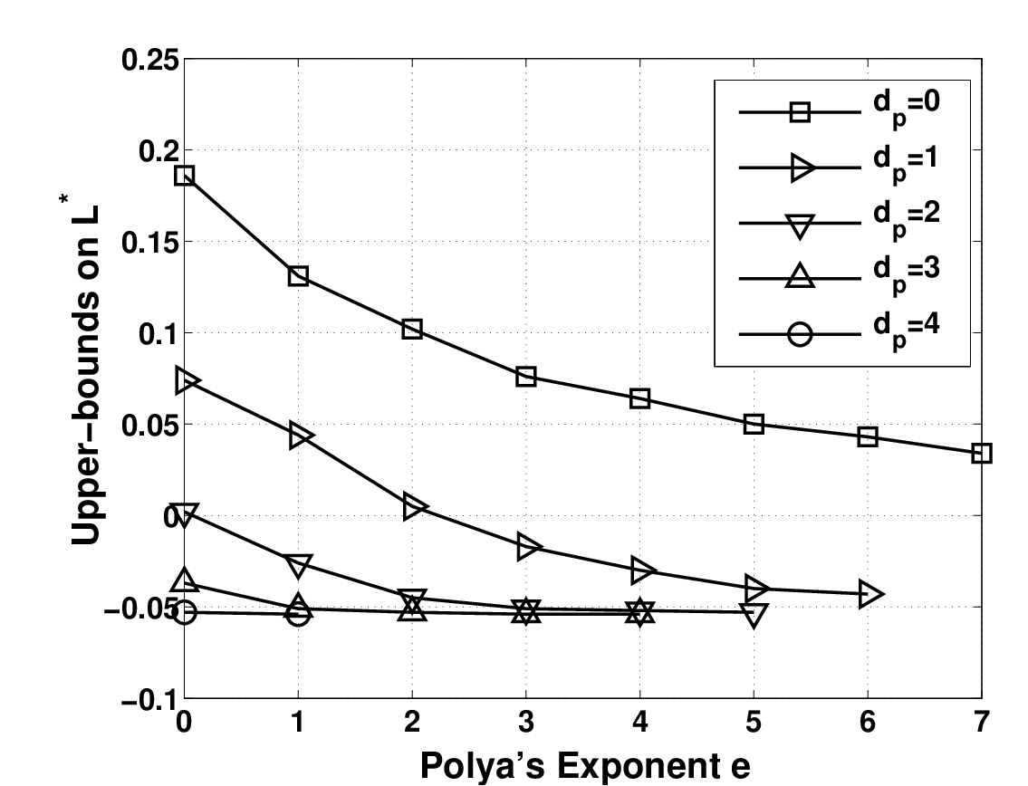
We solved Problem (48) using bisection on LL. For each LL, we used Theorem 3.1 to verify the inequality in (39) using Polya’s exponents e=1e=1 to 7 and dp=1d_{p}=1 to 4 as degrees of PP. Figure 2 shows the computed upper-bounds on L∗L^{*} for different ee and dpd_{p}. The best upper-bound found by the algorithm is −0.0504-0.0504.

Refer to caption
Figure 2. Upper-bounds for L∗L^{*} in Problem (47) for different Polya’s exponents ee and different degrees of PP

For comparison, we solved the same problem using SOSTOOLS [8] and Putinar’s Positivstellensatz (see Case 4 of Section 3.2). By computing a Lyapunov function of degree two in xx and degree one in β\beta, SOSTOOLS certified L=−0.0504L=-0.0504 as an upper-bound for L∗L^{*}. This is the same as the upper-bound computed by Polya’s algorithm. The CPU time required for SOSTOOLS to compute the upper-bound on a Core i7 machine with 64 GB of RAM was 22.3 minutes, whereas the Polya’s algorithm only required 7.1 seconds to compute the same upper-bound.


Case 3. A⁡(α)A(\alpha) is a polynomial with α∈Φl\alpha\in\Phi^{l}:

Given Ah∈ℝn×nA_{h}\in\mathbb{R}^{n\times n} for h∈Edh\in E_{d} as defined in (33), we address the problem of stability analysis of System (30) with A(α)=∑h∈EdAhα1h1⋯αlhlA(\alpha)=\sum_{h\in E_{d}}A_{h}\alpha_{1}^{h_{1}}\cdots\alpha_{l}^{h_{l}} for all α∈Φl:={x∈ℝn:|xi|≤ri}\alpha\in\Phi^{l}:=\{x\in\mathbb{R}^{n}:|x_{i}|\leq r_{i}\}. From Lyapunov theory, System (30) is asymptotically stable for all α∈Φl\alpha\in\Phi^{l} if and only if γ∗>0\gamma^{*}>0 in the following optimization of polynomials problem.

γ∗=maxγ∈ℝ,P∈ℝ⁡[α]⁡γ\displaystyle\gamma^{*}=\max_{\gamma\in\mathbb{R},P\in\mathbb{R}[\alpha]}\;\;\gamma
subject to ​[P⁡(α)00−A​(α)T​P​(α)−P⁡(α)​A​(α)]−γ​I≥0​ for all ​α∈Φl\displaystyle\text{subject to }\begin{bmatrix}P(\alpha)&0\\ 0&-A(\alpha)^{T}P(\alpha)-P(\alpha)A(\alpha)\end{bmatrix}-\gamma I\geq 0\text{ for all }\alpha\in\Phi^{l} (49)

As in Case 2 of Section 3.2, by applying bisection algorithm on γ\gamma and using a multi-simplex version of Polya’s algorithm (such as Theorem 3.2) as a test for feasibility of Constraint (49) we can compute lower bounds on γ∗\gamma^{*}. Suppose there exists a matrix-valued multi-homogeneous polynomial (defined in (17)) QQ of degree vector dq∈ℕld_{q}\in\mathbb{N}^{l} (dqid_{q_{i}} is the degree of βi\beta_{i}) such that

{P(α)∈𝕊n:α∈Φl}={Q(β,η)∈𝕊n:β,η∈ℝl and (βi,ηi)∈Δ2 for i=1,⋯,l}.\{P(\alpha)\in\mathbb{S}^{n}:\alpha\in\Phi^{l}\}=\{Q(\beta,\eta)\in\mathbb{S}^{n}:\beta,\eta\in\mathbb{R}^{l}\text{ and }(\beta_{i},\eta_{i})\in\Delta^{2}\text{ for }i=1,\cdots,l\}. (50)

Likewise, suppose there exists a matrix-valued multi-homogeneous polynomial BB of degree vector db∈ℕld_{b}\in\mathbb{N}^{l} (dbid_{b_{i}} is the degree of βi\beta_{i}) such that

{A(α)∈𝕊n:α∈Φl}={B(β,η)∈𝕊n:β,η∈ℝl and (βi,ηi)∈Δ2 for i=1,⋯,l}.\{A(\alpha)\in\mathbb{S}^{n}:\alpha\in\Phi^{l}\}=\{B(\beta,\eta)\in\mathbb{S}^{n}:\beta,\eta\in\mathbb{R}^{l}\text{ and }(\beta_{i},\eta_{i})\in\Delta^{2}\text{ for }i=1,\cdots,l\}.

Given γ∈ℝ\gamma\in\mathbb{R}, it follows from Theorem 3.2 that the inequality condition in (49) holds for all α∈Φl\alpha\in\Phi^{l} if there exist e≥0e\geq 0 such that

(∏i=1l(βi+ηi)e)​(Q⁡(β,η)−γ​I​(∏i=1l(βi+ηi)dpi))\displaystyle\hskip-14.45377pt\left(\prod_{i=1}^{l}(\beta_{i}+\eta_{i})^{e}\right)\left(Q(\beta,\eta)-\gamma I\left(\prod_{i=1}^{l}(\beta_{i}+\eta_{i})^{d_{p_{i}}}\right)\right) (51)
and
−(∏i=1l(βi+ηi)e)​(BT​(α,β)​Q​(β,η)+Q⁡(β,η)​B​(β,η)+γ​I​(∏i=1l(βi+ηi)dp​ai)),\displaystyle\hskip-25.29494pt-\left(\prod_{i=1}^{l}(\beta_{i}+\eta_{i})^{e}\right)\left(B^{T}(\alpha,\beta)Q(\beta,\eta)+Q(\beta,\eta)B(\beta,\eta)+\gamma I\left(\prod_{i=1}^{l}(\beta_{i}+\eta_{i})^{d_{pa_{i}}}\right)\right), (52)

have all positive coefficients where dpid_{p_{i}} is the degree of αi\alpha_{i} in P⁡(α)P(\alpha) and dp​aid_{pa_{i}} is the degree of αi\alpha_{i} in P⁡(α)​A​(α)P(\alpha)A(\alpha). Suppose QQ and BB are of the forms

Q(β,η)=∑h,g∈ℕlh+g=dqQh,gβ1h1η1g1⋯βlhlηlglQ(\beta,\eta)=\sum_{\begin{subarray}{c}h,g\in\mathbb{N}^{l}\\ h+g=d_{q}\end{subarray}}Q_{h,g}\beta_{1}^{h_{1}}\eta_{1}^{g_{1}}\cdots\beta_{l}^{h_{l}}\eta_{l}^{g_{l}} (53)

and

B(β,η)=∑h,g∈ℕlh+g=dbBh,gβ1h1η1g1⋯βlhlηlgl.B(\beta,\eta)=\sum_{\begin{subarray}{c}h,g\in\mathbb{N}^{l}\\ h+g=d_{b}\end{subarray}}B_{h,g}\beta_{1}^{h_{1}}\eta_{1}^{g_{1}}\cdots\beta_{l}^{h_{l}}\eta_{l}^{g_{l}}. (54)

By combining (53) and (54) with (51) and (52) we find that for a given γ∈ℝ\gamma\in\mathbb{R}, the inequality condition in (49) holds for all α∈Φl\alpha\in\Phi^{l} if there exist some e≥0e\geq 0 such that

∑h,g∈ℕlh+g=dqf{q,r},{h,g}​Qh,g>0​ for all ​q,r∈ℕl:q+r=dq+e⋅𝟏​ and\displaystyle\sum_{\begin{subarray}{c}h,g\in\mathbb{N}^{l}\\ h+g=d_{q}\end{subarray}}\hskip-4.33601ptf_{\{q,r\},\{h,g\}}Q_{h,g}>0\;\;\text{ for all }\;q,r\in\mathbb{N}^{l}:q+r=d_{q}+e\cdot\mathbf{1}\;\;\text{ and}
∑h,g∈ℕlh+g=dqM{s,t},{h,g}T​Qh,g+Qh,g​M{s,t},{h,g}<0​ for all ​s,t∈ℕl:s+t=dq+db+e⋅𝟏,\displaystyle\sum_{\begin{subarray}{c}h,g\in\mathbb{N}^{l}\\ h+g=d_{q}\end{subarray}}\hskip-5.78172ptM_{\{s,t\},\{h,g\}}^{T}Q_{h,g}+Q_{h,g}M_{\{s,t\},\{h,g\}}\hskip-2.168pt<0\text{ for all }s,t\in\mathbb{N}^{l}\hskip-2.168pt:\hskip-2.168pts+t=d_{q}+d_{b}+e\cdot\mathbf{1}, (55)

where 𝟏∈ℕl\mathbf{1}\in\mathbb{N}^{l} is the vector of ones and where we define f{q,r},{h,g}∈ℝf_{\{q,r\},\{h,g\}}\in\mathbb{R} to be the coefficient of Qh,g​βq​ηrQ_{h,g}\beta^{q}\eta^{r} after expansion of (51). Likewise, we define M{s,t},{h,g}∈ℝn×nM_{\{s,t\},\{h,g\}}\in\mathbb{R}^{n\times n} to be the coefficient of Qh,g​βs​ηtQ_{h,g}\beta^{s}\eta^{t} after expansion of (52). See [34] for recursive formulae for calculating f{q,r},{h,g}f_{\{q,r\},\{h,g\}} and M{s,t},{h,g}M_{\{s,t\},\{h,g\}}. Similar to Case 2, Conditions (55) are an SDP (See [34] for a complexity analysis on this SDP). For any γ∈ℝ\gamma\in\mathbb{R}, if there exist e≥0e\geq 0 and {Qh,g}\{Q_{h,g}\} that satisfy (55), then γ≤γ∗\gamma\leq\gamma^{*} as defined in (49). Furthermore, if γ\gamma is positive, then x˙​(t)=A​(α)​x​(t)\dot{x}(t)=A(\alpha)x(t) is asymptotically stable for all α∈Φl\alpha\in\Phi^{l}.


Numerical Example 3a: Consider the system x˙​(t)=A​(α)​x​(t)\dot{x}(t)=A(\alpha)x(t), where

A⁡(α)=A0+A1​α12+A2​α1​α2​α3+A3​α12​α2​α32,A(\alpha)=A_{0}+A_{1}\alpha_{1}^{2}+A_{2}\alpha_{1}\alpha_{2}\alpha_{3}+A_{3}\alpha_{1}^{2}\alpha_{2}\alpha_{3}^{2},
α1∈[−1,1],α2∈[−0.5,0.5],α3∈[−0.1,0.1],\alpha_{1}\in[-1,1],\,\alpha_{2}\in[-0.5,0.5],\,\alpha_{3}\in[-0.1,0.1],

where

A0=[−3.00−1.73.0−0.2−2.9−1.7−2.60.62.6−5.8−2.6−0.72.9−3.3−2.1]​A1=[2.2−5.4−0.8−2.24.41.4−3.00.8−2.4−2.21.46.0−2.4−4.4−6.40.18]\displaystyle A_{0}=\begin{bmatrix}-3.0&0&-1.7&3.0\\ -0.2&-2.9&-1.7&-2.6\\ 0.6&2.6&-5.8&-2.6\\ -0.7&2.9&-3.3&-2.1\end{bmatrix}A_{1}=\begin{bmatrix}2.2&-5.4&-0.8&-2.2\\ 4.4&1.4&-3.0&0.8\\ -2.4&-2.2&1.4&6.0\\ -2.4&-4.4&-6.4&0.18\end{bmatrix}
A2=[−8.0−13.5−0.5−3.018.0−2.00.5−11.55.5−10.03.59.013.07.55.0−4.0]​A3=[3.07.52.5−8.01.00.51.01.5−0.5−1.01.06.0−2.5−6.08.514.25].\displaystyle A_{2}=\begin{bmatrix}-8.0&-13.5&-0.5&-3.0\\ 18.0&-2.0&0.5&-11.5\\ 5.5&-10.0&3.5&9.0\\ 13.0&7.5&5.0&-4.0\end{bmatrix}A_{3}=\begin{bmatrix}3.0&7.5&2.5&-8.0\\ 1.0&0.5&1.0&1.5\\ -0.5&-1.0&1.0&6.0\\ -2.5&-6.0&8.5&14.25\end{bmatrix}.

The problem is to investigate asymptotic stability of this system for all α\alpha in the given intervals using the method in Case 3 of Section 4.1. We first represented A⁡(α)A(\alpha) over [−1,1]×[−0.5,0.5]×[−0.1,0.1][-1,1]\times[-0.5,0.5]\times[-0.1,0.1] by a multi-homogeneous polynomial B⁡(β,η)B(\beta,\eta) with (βi,ηi)∈Δ2(\beta_{i},\eta_{i})\in\Delta^{2} and with the degree vector db=[2,1,2]d_{b}=[2,1,2] (see [34] for an algorithm which finds BB and see Case 2 of Section (3.2) for an example). Then, by applying Theorem 3.2 (as in (51) and (52)) with γ=0.1,e=1\gamma=0.1,e=1 and dp=[1,1,1]d_{p}=[1,1,1], we set-up the inequalities in (55) with dq=[1,1,1]d_{q}=[1,1,1]. By using semi-definite programming, we solved the inequalities and computed the following Lyapunov function as a certificate for asymptotic stability of x˙​(t)=A​(α)​x​(t)\dot{x}(t)=A(\alpha)x(t) for all α1∈[−1,1],α2∈[−0.5,0.5],α3∈[−0.1,0.1]\alpha_{1}\in[-1,1],\,\alpha_{2}\in[-0.5,0.5],\,\alpha_{3}\in[-0.1,0.1].

V⁡(x,β,η)=xT​Q​(β,η)​x=xT​(CLOSE\displaystyle V(x,\beta,\eta)=x^{T}Q(\beta,\eta)x=x^{T}( β1​(Q1​β2​β3+Q2​β2​η3+Q3​η2​β3+Q4​η2​η3)\displaystyle\beta_{1}(Q_{1}\beta_{2}\beta_{3}+Q_{2}\beta_{2}\eta_{3}+Q_{3}\eta_{2}\beta_{3}+Q_{4}\eta_{2}\eta_{3})
+\displaystyle+ OPENη1​(Q5​β2​β3+Q6​β2​η3+Q7​η2​β3+Q8​η2​η3))​x,\displaystyle\eta_{1}(Q_{5}\beta_{2}\beta_{3}+Q_{6}\beta_{2}\eta_{3}+Q_{7}\eta_{2}\beta_{3}+Q_{8}\eta_{2}\eta_{3}))x,

where β1=0.5​α1+0.5,β2=α2+0.5,β3=5​α3+0.5,η1=1−β1,η2=1−β2,η3=1−β3\beta_{1}=0.5\alpha_{1}+0.5,\beta_{2}=\alpha_{2}+0.5,\beta_{3}=5\alpha_{3}+0.5,\eta_{1}=1-\beta_{1},\eta_{2}=1-\beta_{2},\eta_{3}=1-\beta_{3} and

Q1=[5.8070.010−0.187−1.1860.0105.042−0.3690.227−0.187−0.3698.227−1.824−1.1860.227−1.8248.127]​Q2=[7.409−0.8031.804−1.594−0.8036.0160.042−0.5381.8040.0427.894−1.118−1.594−0.538−1.1188.590]\displaystyle Q_{1}=\begin{bmatrix}5.807&0.010&-0.187&-1.186\\ 0.010&5.042&-0.369&0.227\\ -0.187&-0.369&8.227&-1.824\\ -1.186&0.227&-1.824&8.127\end{bmatrix}Q_{2}=\begin{bmatrix}7.409&-0.803&1.804&-1.594\\ -0.803&6.016&0.042&-0.538\\ 1.804&0.042&7.894&-1.118\\ -1.594&-0.538&-1.118&8.590\end{bmatrix}
Q3=[6.095−0.8730.512−1.125−0.8735.934−0.1610.5030.512−0.1617.417−0.538−1.1250.503−0.5386.896]​Q4=[5.3880.130−0.363−0.3330.1305.044−0.113−0.117−0.363−0.1136.156−0.236−0.333−0.117−0.2365.653]\displaystyle Q_{3}=\begin{bmatrix}6.095&-0.873&0.512&-1.125\\ -0.873&5.934&-0.161&0.503\\ 0.512&-0.161&7.417&-0.538\\ -1.125&0.503&-0.538&6.896\end{bmatrix}Q_{4}=\begin{bmatrix}5.388&0.130&-0.363&-0.333\\ 0.130&5.044&-0.113&-0.117\\ -0.363&-0.113&6.156&-0.236\\ -0.333&-0.117&-0.236&5.653\end{bmatrix}
Q5=[7.410−0.8031.804−1.594−0.8036.0160.042−0.5381.8040.0427.894−1.118−1.594−0.538−1.1188.590]​Q6=[5.8070.010−0.187−1.1860.0105.042−0.3690.227−0.187−0.3698.227−1.824−1.1860.227−1.8248.127]\displaystyle Q_{5}=\begin{bmatrix}7.410&-0.803&1.804&-1.594\\ -0.803&6.016&0.042&-0.538\\ 1.804&0.042&7.894&-1.118\\ -1.594&-0.538&-1.118&8.590\end{bmatrix}Q_{6}=\begin{bmatrix}5.807&0.010&-0.187&-1.186\\ 0.010&5.042&-0.369&0.227\\ -0.187&-0.369&8.227&-1.824\\ -1.186&0.227&-1.824&8.127\end{bmatrix}
Q7=[5.3880.130−0.363−0.3330.1305.044−0.113−0.117−0.363−0.1136.156−0.236−0.333−0.117−0.2365.653]​Q8=[6.095−0.8730.512−1.125−0.8735.934−0.1610.5030.512−0.1617.417−0.538−1.1250.503−0.5386.896].\displaystyle Q_{7}=\begin{bmatrix}5.388&0.130&-0.363&-0.333\\ 0.130&5.044&-0.113&-0.117\\ -0.363&-0.113&6.156&-0.236\\ -0.333&-0.117&-0.236&5.653\end{bmatrix}Q_{8}=\begin{bmatrix}6.095&-0.873&0.512&-1.125\\ -0.873&5.934&-0.161&0.503\\ 0.512&-0.161&7.417&-0.538\\ -1.125&0.503&-0.538&6.896\end{bmatrix}.

Numerical Example 3b: In this example, we used the same method as in Example 3a to find lower bounds on r∗=max⁡rr^{*}=\max\,r such that x˙​(t)=A​(α)​x​(t)\dot{x}(t)=A(\alpha)x(t) with

A⁡(α)=A0+∑i=14Ai​αi,A(\alpha)=A_{0}+\sum_{i=1}^{4}A_{i}\alpha_{i},
A0=[−3.00−1.73.0−0.2−2.9−1.7−2.60.62.6−5.8−2.6−0.72.9−3.3−2.4]​A1=[1.1−2.7−0.4−1.12.20.7−1.50.4−1.2−1.10.73.0−1.2−2.2−3.2−1.4]\displaystyle A_{0}=\begin{bmatrix}-3.0&0&-1.7&3.0\\ -0.2&-2.9&-1.7&-2.6\\ 0.6&2.6&-5.8&-2.6\\ -0.7&2.9&-3.3&-2.4\end{bmatrix}A_{1}=\begin{bmatrix}1.1&-2.7&-0.4&-1.1\\ 2.2&0.7&-1.5&0.4\\ -1.2&-1.1&0.7&3.0\\ -1.2&-2.2&-3.2&-1.4\end{bmatrix}
A2=[1.62.70.10.6−3.60.4−0.12.3−1.12−0.7−1.8−2.6−1.5−1.00.8]​A3=[−0.61.50.5−1.60.2−0.10.20.3−0.1−0.2−0.21.2−0.5−1.21.7−0.1]\displaystyle A_{2}=\begin{bmatrix}1.6&2.7&0.1&0.6\\ -3.6&0.4&-0.1&2.3\\ -1.1&2&-0.7&-1.8\\ -2.6&-1.5&-1.0&0.8\end{bmatrix}A_{3}=\begin{bmatrix}-0.6&1.5&0.5&-1.6\\ 0.2&-0.1&0.2&0.3\\ -0.1&-0.2&-0.2&1.2\\ -0.5&-1.2&1.7&-0.1\end{bmatrix}
A4=[−0.4−0.1−0.30.10.10.30.20.00.00.2−0.30.10.1−0.2−0.20.0].\displaystyle\hskip 18.49988pt\hskip 18.49988pt\hskip 18.49988pt\hskip 18.49988ptA_{4}=\begin{bmatrix}-0.4&-0.1&-0.3&0.1\\ 0.1&0.3&0.2&0.0\\ 0.0&0.2&-0.3&0.1\\ 0.1&-0.2&-0.2&0.0\end{bmatrix}.

is asymptotically stable for all α∈{α∈ℝ4:|αi|≤r}\alpha\in\{\alpha\in\mathbb{R}^{4}:|\alpha_{i}|\leq r\}. Table 1 shows the computed lower bounds on r∗r^{*} for different degree vectors dqd_{q} (degree vector of QQ in (50)). In all of the cases, we set the Polya’s exponent e=0e=0. For comparison, we have also included the lower-bounds computed by the methods of [72] and [73] in Table 1.

Table 1. The lower-bounds on r∗r^{*} computed by the method in Case 3 of Section 4.1 and methods in [72] and [73] - it​hi^{th} entry of dqd_{q} is the degree of βi\beta_{i} in (50)
dq=d_{q}=[0,0,0,0] dq=d_{q}=[0,1,0,1] dq=d_{q}=[1,0,1,0] dq=d_{q}=[1,1,1,1] dq=d_{q}=[2,2,2,2] Ref.[72] Ref.[73]
bound on r∗r^{*} 0.494 0.508 0.615 0.731 0.840 0.4494 0.8739

4.2. Nonlinear stability analysis

Consider nonlinear systems of the form

x˙​(t)=f​(x​(t)),\dot{x}(t)=f(x(t)), (56)

where f:ℝn→ℝnf:\mathbb{R}^{n}\rightarrow\mathbb{R}^{n} is a degree dfd_{f} polynomial. Suppose the origin is an isolated equilibrium of (56). In this section, we address local stability of the origin in the following sense.

Lemma 4.1.

Consider the System (56) and let Q⊂ℝn×nQ\subset\mathbb{R}^{n\times n} be an open set containing the origin. Suppose there exists a continuously differentiable function VV which satisfies

V⁡(x)>0​ for all ​x∈Q∖{0},V⁡(0)=0V(x)>0\text{ for all }x\in Q\setminus\{0\},V(0)=0 (57)

and

⟨∇V,f⁡(x)⟩<0​ for all ​x∈Q∖{0}.\langle\nabla V,f(x)\rangle<0\text{ for all }x\in Q\setminus\{0\}. (58)

Then the origin is an asymptotically stable equilibrium of System (56), meaning that for every x⁡(0)∈{x∈ℝn:{y:V⁡(y)≤V⁡(x)}⊂Q}x(0)\in\{x\in\mathbb{R}^{n}:\{y:V(y)\leq V(x)\}\subset Q\}, limt→∞x⁡(t)=0\lim_{t\to\infty}x(t)=0.

Since existence of polynomial Lyapunov functions is necessary and sufficient for stability of (56) on any compact set [74], we can formulate the problem of stability analysis of (56) as follows.

γ∗=maxγ,cβ∈ℝ⁡γ\displaystyle\gamma^{*}=\max_{\gamma,c_{\beta}\in\mathbb{R}}\;\;\gamma
subject to​[∑β∈Edcβ​xβ−γ​xT​x00−⟨∇∑β∈Edcβxβ,f(x)⟩−γxTx]≥0​ for all ​x∈Q.\displaystyle\text{subject to}\begin{bmatrix}\sum_{\beta\in E_{d}}c_{\beta}x^{\beta}-\gamma x^{T}x&0\\ 0&\hskip-7.22743pt-\langle\nabla\sum_{\beta\in E_{d}}c_{\beta}x^{\beta},f(x)\rangle-\gamma x^{T}x\end{bmatrix}\geq 0\text{ for all }x\in Q. (59)

Conditions (57) and (58) hold if and only if there exist d∈ℕd\in\mathbb{N} such that γ∗>0\gamma^{*}>0. In Sections 4.2.1 and 4.2.2, we discuss two alternatives to SOS programming for solving (59). These methods apply Polya’s theorem and Handelman’s theorem to Problem (59) (as described in Cases 2 and 3 in Section 3.2) to find lower bounds on γ∗\gamma^{*}. See [43] for a different application of Handelman’s theorem and intervals method in nonlinear stability. Also, see [41] for a method of computing continuous piecewise affine Lyapunov functions using linear programming and a triangulation scheme for polytopes.

4.2.1. Application of Handelman’s theorem in nonlinear stability analysis

Recall that every convex polytope can be represented as

ΓK:={x∈ℝn:wiTx+ui≥0,i=1,⋯,K}\Gamma^{K}:=\{x\in\mathbb{R}^{n}:w_{i}^{T}x+u_{i}\geq 0,i=1,\cdots,K\} (60)

for some wi∈ℝnw_{i}\in\mathbb{R}^{n} and ui∈ℝu_{i}\in\mathbb{R}. Suppose ΓK\Gamma^{K} is bounded and the origin is in the interior of ΓK\Gamma^{K}. In this section, we would like to investigate asymptotic stability of the equilibrium of System (56) by verifying positivity of γ∗\gamma^{*} in Problem (59) with Q=ΓKQ=\Gamma^{K}.

Unfortunately, Handelman’s theorem (Theorem 2.4) does not parameterize polynomials which have zeros in the interior of a given polytope. To see this, suppose a polynomial gg (gg is not identically zero) is zero at x=ax=a, where aa is in the interior of a polytope ΓK:={x∈ℝn:wiTx+ui≥0,i=1,⋯,K}\Gamma^{K}:=\{x\in\mathbb{R}^{n}:w_{i}^{T}x+u_{i}\geq 0,i=1,\cdots,K\}. Suppose there exist bα≥0,α∈ℕKb_{\alpha}\geq 0,\alpha\in\mathbb{N}^{K} such that for some d∈ℕd\in\mathbb{N},

g(x)=∑α∈ℕK‖αi‖1≤dbα(w1Tx+u1)α1⋯(wKTx+uK)αK.g(x)=\sum_{\begin{subarray}{c}\alpha\in\mathbb{N}^{K}\\ \|\alpha_{i}\|_{1}\leq d\end{subarray}}b_{\alpha}(w_{1}^{T}x+u_{1})^{\alpha_{1}}\cdots(w_{K}^{T}x+u_{K})^{\alpha_{K}}.

Then,

g(a)=∑α∈ℕK‖αi‖1≤dbα(w1Ta+u1)α1⋯(wKTa+uK)αK=0.g(a)=\sum_{\begin{subarray}{c}\alpha\in\mathbb{N}^{K}\\ \|\alpha_{i}\|_{1}\leq d\end{subarray}}b_{\alpha}(w_{1}^{T}a+u_{1})^{\alpha_{1}}\cdots(w_{K}^{T}a+u_{K})^{\alpha_{K}}=0.

From the assumption a∈int​(ΓK)a\in\text{int}(\Gamma^{K}) it follows that wiT​a+ui>0w_{i}^{T}a+u_{i}>0 for i=1,⋯,Ki=1,\cdots,K. Hence bα<0b_{\alpha}<0 for at least one α∈{α∈ℕK:‖α‖1≤d}\alpha\in\{\alpha\in\mathbb{N}^{K}:\|\alpha\|_{1}\leq d\}. This contradicts with the assumption that all bα≥0b_{\alpha}\geq 0.

Based on the above reasoning, one cannot readily use Handelman’s theorem to verify the Lyapunov inequalities in (57). In [44], a combination of Handelman’s theorem and a decomposition scheme was applied to Problem (59) with Q=ΓKQ=\Gamma^{K}. Here we outline this result. First, consider the following definitions.

Definition 4.2.

Given a bounded polytope of the form ΓK:={x∈ℝn:wiTx+ui≥0,i=1,⋯,K}\Gamma^{K}:=\{x\in\mathbb{R}^{n}:w_{i}^{T}x+u_{i}\geq 0,i=1,\cdots,K\}, we call

ζi​(ΓK):={x∈ℝn:wiT​x+ui=0​ and ​wjT​x+uj≥0​ for ​j∈{1,⋯,K}}\zeta^{i}(\Gamma^{K}):=\{x\in\mathbb{R}^{n}:w_{i}^{T}x+u_{i}=0\text{ and }w_{j}^{T}x+u_{j}\geq 0\text{ for }j\in\{1,\cdots,K\}\}

the i−i-th facet of ΓK\Gamma^{K} if ζi​(ΓK)≠∅\zeta^{i}(\Gamma^{K})\neq\emptyset.

Definition 4.3.

Given a bounded polytope of the form ΓK:={x∈ℝn:wiTx+ui≥0,i=1,⋯,K}\Gamma^{K}:=\{x\in\mathbb{R}^{n}:w_{i}^{T}x+u_{i}\geq 0,i=1,\cdots,K\}, we call DΓ:={Di}i=1,⋯,LD_{\Gamma}:=\{D_{i}\}_{i=1,\cdots,L} a D−D-decomposition of ΓK\Gamma^{K} if

Di:={x∈ℝn:hi,jTx+gi,j≥0,j=1,⋯,mi} for some hi,j∈ℝn,gi,j∈ℝD_{i}:=\{x\in\mathbb{R}^{n}:h^{T}_{i,j}x+g_{i,j}\geq 0,j=1,\cdots,m_{i}\}\;\;\text{ for some }h_{i,j}\in\mathbb{R}^{n},\,g_{i,j}\in\mathbb{R}

such that ∪i=1LDi=ΓK,∩i=1LDi={0}\cup_{i=1}^{L}D_{i}=\Gamma^{K},\,\cap_{i=1}^{L}D_{i}=\{0\} and int​(Di)∩int​(Dj)=∅\text{int}(D_{i})\cap\text{int}(D_{j})=\emptyset.

Consider System (56) with polynomial ff of degree dfd_{f}. Given wi,hi,j∈ℝnw_{i},h_{i,j}\in\mathbb{R}^{n} and ui,gi,j∈ℝu_{i},g_{i,j}\in\mathbb{R}, let ΓK:={x∈ℝn:wiTx+ui≥0,i=1,⋯,K}\Gamma^{K}:=\{x\in\mathbb{R}^{n}:w_{i}^{T}x+u_{i}\geq 0,i=1,\cdots,K\} with D−D-decomposition DΓ:={Di}i=1,⋯,LD_{\Gamma}:=\{D_{i}\}_{i=1,\cdots,L}, where Di:={x∈ℝn:hi,jTx+gi,j≥0,j=1,⋯,mi}D_{i}:=\{x\in\mathbb{R}^{n}:h^{T}_{i,j}x+g_{i,j}\geq 0,j=1,\cdots,m_{i}\}. Let us denote the elements of the set

Ed,n:={α∈ℕn:∑i=1nαi≤d}E_{d,n}:=\{\alpha\in\mathbb{N}^{n}:\sum_{i=1}^{n}\alpha_{i}\leq d\}

by λ(k),k=1,⋯,B\lambda^{(k)},k=1,\cdots,B, where BB is the cardinality of Ed,eE_{d,e}. For any λ(k)\lambda^{(k)}, let p{λ(k),α,i}p_{\{\lambda^{(k)},\alpha,i\}} be the coefficient of bi,α​xλ(k)b_{i,\alpha}\,x^{\lambda^{(k)}} in

Pi​(x):=∑α∈Ed,mibi,α​∏j=1mi(hi,jT​x+gi,j)αj,x∈ℝn,bi,α∈ℝ.P_{i}(x):=\sum_{\alpha\in E_{d,m_{i}}}b_{i,\alpha}\prod_{j=1}^{m_{i}}(h_{i,j}^{T}x+g_{i,j})^{\alpha_{j}},\;x\in\mathbb{R}^{n},b_{i,\alpha}\in\mathbb{R}. (61)

Let us denote the cardinality of Ed,miE_{d,m_{i}} by NiN_{i} and denote the vector of all coefficients bi,αb_{i,\alpha} by bi∈ℝNib_{i}\in\mathbb{R}^{N_{i}}. Define the map Fi:ℝNi×ℕ→ℝBF_{i}:\mathbb{R}^{N_{i}}\times\mathbb{N}\rightarrow\mathbb{R}^{B} as

Fi​(bi,d):=[∑α∈Ed,mip{λ(1),α,i}​bi,α,⋯,∑α∈Ed,mip{λ(B),α,i}​bi,α]TF_{i}(b_{i},d):=\left[\sum_{\begin{subarray}{c}\alpha\in E_{d,m_{i}}\end{subarray}}p_{\{\lambda^{(1)},\alpha,i\}}b_{i,\alpha}\;,\;\cdots\;,\;\sum_{\begin{subarray}{c}\alpha\in E_{d,m_{i}}\end{subarray}}p_{\{\lambda^{(B)},\alpha,i\}}b_{i,\alpha}\right]^{T}

for i=1,⋯,Li=1,\cdots,L. In other words, Fi​(bi,d)F_{i}(b_{i},d) is the vector of coefficients of Pi​(x)P_{i}(x) after expansion.

Define Hi:ℝNi×ℕ→ℝQH_{i}:\mathbb{R}^{N_{i}}\times\mathbb{N}\rightarrow\mathbb{R}^{Q} as

Hi​(bi,d):=[∑α∈Ed,mip{δ(1),α,i}​bi,α,⋯,∑α∈Ed,mip{δ(Q),α,i}​bi,α]TH_{i}(b_{i},d):=\left[\sum_{\begin{subarray}{c}\alpha\in E_{d,m_{i}}\end{subarray}}p_{\{\delta^{(1)},\alpha,i\}}b_{i,\alpha}\;,\;\cdots\;,\;\sum_{\begin{subarray}{c}\alpha\in E_{d,m_{i}}\end{subarray}}p_{\{\delta^{(Q)},\alpha,i\}}b_{i,\alpha}\right]^{T}

for i=1,⋯,Li=1,\cdots,L, where we have denoted the elements of {δ∈ℕn:δ=2ej for j=1,⋯,n}\{\delta\in\mathbb{N}^{n}:\delta=2e_{j}\text{ for }j=1,\cdots,n\} by δ(k),k=1,⋯,Q\delta^{(k)},k=1,\cdots,Q, where eje_{j} are the canonical basis for ℕn\mathbb{N}^{n}. In other words, Hi​(bi,d)H_{i}(b_{i},d) is the vector of coefficients of square terms of Pi​(x)P_{i}(x) after expansion.

Define Ri​(bi,d):ℝNi×ℕ→ℝCR_{i}(b_{i},d):\mathbb{R}^{N_{i}}\times\mathbb{N}\rightarrow\mathbb{R}^{C} as

Ri​(bi,d):=[bi,β(1),⋯,bi,β(C)]T,R_{i}(b_{i},d):=\left[b_{i,\beta^{(1)}}\;,\;\cdots\;,\;b_{i,\beta^{(C)}}\right]^{T},

for i=1,⋯,Li=1,\cdots,L, where we have denoted the elements of the set

{β∈Ed,mi:βj=0​ for ​j∈{j∈ℕ:gi,j=0}}\{\beta\in E_{d,m_{i}}:\beta_{j}=0\text{ for }j\in\{j\in\mathbb{N}:g_{i,j}=0\}\}

by β(k)\beta^{(k)} for k=1,⋯,Ck=1,\cdots,C.

Define Ji:ℝNi×ℕ×{1,⋯,mi}→ℝBJ_{i}:\mathbb{R}^{N_{i}}\times\mathbb{N}\times\{1,\cdots,m_{i}\}\rightarrow\mathbb{R}^{B} as

Ji​(bi,d,k):=[∑α∈Ed,miαk=0p{λ(1),α,i}​bi,α,⋯,∑α∈Ed,miαk=0p{λ(B),α,i}​bi,α]TJ_{i}(b_{i},d,k):=\left[\sum_{\begin{subarray}{c}\alpha\in E_{d,m_{i}}\\ \alpha_{k}=0\end{subarray}}p_{\{\lambda^{(1)},\alpha,i\}}b_{i,\alpha}\;,\;\cdots\;,\;\sum_{\begin{subarray}{c}\alpha\in E_{d,m_{i}}\\ \alpha_{k}=0\end{subarray}}p_{\{\lambda^{(B)},\alpha,i\}}b_{i,\alpha}\right]^{T}

for i,k=1,⋯,Li,k=1,\cdots,L. In other words, Ji​(bi,d,k)J_{i}(b_{i},d,k) is the vector of coefficients of restriction of PiP_{i} to hi,kT​x+gi,k=0h_{i,k}^{T}x+g_{i,k}=0, after expansion.

Define Gi:ℝNi×ℕ→ℝZG_{i}:\mathbb{R}^{N_{i}}\times\mathbb{N}\rightarrow\mathbb{R}^{Z} as

Gi​(bi,d):=[∑α∈Ed,miq{η(1),α,i}​bi,α,⋯,∑α∈Ed,miq{η(P),α,i}​bi,α]TG_{i}(b_{i},d):=\left[\sum_{\begin{subarray}{c}\alpha\in E_{d,m_{i}}\end{subarray}}q_{\{\eta^{(1)},\alpha,i\}}b_{i,\alpha}\;,\;\cdots\;,\;\sum_{\begin{subarray}{c}\alpha\in E_{d,m_{i}}\end{subarray}}q_{\{\eta^{(P)},\alpha,i\}}b_{i,\alpha}\right]^{T}

for i=1,⋯,Li=1,\cdots,L, where we have denoted the elements of Ed+df−1,nE_{d+d_{f}-1,n} by η(k)\eta^{(k)} for k=1,⋯,Zk=1,\cdots,Z. For any η(k)∈Ed+df−1,n\eta^{(k)}\in E_{d+d_{f}-1,n}, we define q{η(k),α,i}q_{\{\eta^{(k)},\alpha,i\}} as the coefficient of bi,α​xη(k)b_{i,\alpha}\,x^{\eta^{(k)}} in ⟨∇Pi​(x),f⁡(x)⟩\langle\nabla P_{i}(x),f(x)\rangle, where Pi​(x)P_{i}(x) is defined in (61).

Finally, given i,j∈{1,⋯,L},i≠ji,j\in\{1,\cdots,L\},i\neq j, let

Λi,j:={k,l∈ℕ:k∈{1,⋯,mi},l∈{1,⋯,mj}:ζk(Di)≠∅ and ζk(Di)=ζl(Dj)}\Lambda_{i,j}:=\left\{k,l\in\mathbb{N}:k\in\{1,\cdots,m_{i}\},l\in\{1,\cdots,m_{j}\}:\zeta^{k}(D_{i})\neq\emptyset\text{ and }\zeta^{k}(D_{i})=\zeta^{l}(D_{j})\right\}

If there exist d∈ℕd\in\mathbb{N} such that max⁡γ\max\gamma in the linear program

maxγ∈ℝ,bi∈ℝNi,ci∈ℝMi⁡γ\displaystyle\max_{\gamma\in\mathbb{R},b_{i}\in\mathbb{R}^{N_{i}},c_{i}\in\mathbb{R}^{M_{i}}}\;\;\;\gamma
subject to ​bi≥𝟎\displaystyle\text{subject to }\;\;b_{i}\geq\mathbf{0} for ​i=1,⋯,L\displaystyle\text{ for }i=1,\cdots,L
ci≤𝟎\displaystyle\hskip 52.75679ptc_{i}\leq\mathbf{0} for ​i=1,⋯,L\displaystyle\text{ for }i=1,\cdots,L
Ri​(bi,d)=𝟎\displaystyle\hskip 52.75679ptR_{i}(b_{i},d)=\mathbf{0} for ​i=1,⋯,L\displaystyle\text{ for }i=1,\cdots,L
Hi​(bi,d)≥γ⋅𝟏\displaystyle\hskip 52.75679ptH_{i}(b_{i},d)\geq\gamma\cdot\mathbf{1} for ​i=1,⋯,L\displaystyle\text{ for }i=1,\cdots,L
Hi(ci,d+df−1)≤−γ⋅𝟏\displaystyle\hskip 52.75679ptH_{i}(c_{i},d+d_{f}-1)\leq-\gamma\cdot\mathbf{1} for ​i=1,⋯,L\displaystyle\text{ for }i=1,\cdots,L
Gi​(bi,d)=Fi​(ci,d+df−1)\displaystyle\hskip 52.75679ptG_{i}(b_{i},d)=F_{i}(c_{i},d+d_{f}-1) for ​i=1,⋯,L\displaystyle\text{ for }i=1,\cdots,L
Ji​(bi,d,k)=Jj​(bj,d,l)\displaystyle\hskip 52.75679ptJ_{i}(b_{i},d,k)=J_{j}(b_{j},d,l) for ​i,j=1,⋯,L​ and ​k,l∈Λi,j\displaystyle\text{ for }i,j=1,\cdots,L\text{ and }k,l\in\Lambda_{i,j} (62)

is positive, then the origin is an asymptotically stable equilibrium for System (56) and

V(x)=Vi(x)=∑α∈Ed,mibi,α∏j=1mi(hi,jTx+gi,j)αj for x∈Di,i=1,⋯,LV(x)=V_{i}(x)=\sum_{\begin{subarray}{c}\alpha\in E_{d,m_{i}}\end{subarray}}b_{i,\alpha}\prod_{j=1}^{m_{i}}(h^{T}_{i,j}x+g_{i,j})^{\alpha_{j}}\;\text{ for }x\in D_{i},i=1,\cdots,L

is a piecewise polynomial Lyapunov function proving stability of System (56). See [44] for a comprehensive discussion on the computational complexity of the LP defined in (62) in terms of the state-space dimension and the degree of V⁡(x)V(x).


Numerical Example 4: Consider the following nonlinear system [76].

x˙1=x2\displaystyle\dot{x}_{1}=x_{2}
x˙2=−2​x1−x2+x1​x22−x15+x1​x24+x25.\displaystyle\dot{x}_{2}=-2x_{1}-x_{2}+x_{1}x_{2}^{2}-x_{1}^{5}+x_{1}x_{2}^{4}+x_{2}^{5}.

Using the polytope

Γ4={x1,x2∈ℝ2:\displaystyle\Gamma^{4}=\{x_{1},x_{2}\in\mathbb{R}^{2}:\, 1.428​x1+x2−0.625≥0,−1.428​x1+x2+0.625≥0,\displaystyle 1.428x_{1}+x_{2}-0.625\geq 0,-1.428x_{1}+x_{2}+0.625\geq 0,
1.428x1+x2+0.625≥0,−1.428x1+x2−0.625≥0},\displaystyle 1.428x_{1}+x_{2}+0.625\geq 0,-1.428x_{1}+x_{2}-0.625\geq 0\}, (63)

and D−D-decomposition

D1:={x1,x2∈ℝ2:−x1≥0,x2≥0,−1.428x1+x2−0.625≥0}\displaystyle D_{1}:=\{x_{1},x_{2}\in\mathbb{R}^{2}:-x_{1}\geq 0,x_{2}\geq 0,-1.428x_{1}+x_{2}-0.625\geq 0\}
D2:={x1,x2∈ℝ2:x1≥0,x2≥0,1.428x1+x2+0.625≥0}\displaystyle D_{2}:=\{x_{1},x_{2}\in\mathbb{R}^{2}:x_{1}\geq 0,x_{2}\geq 0,1.428x_{1}+x_{2}+0.625\geq 0\}
D3:={x1,x2∈ℝ2:x1≥0,−x2≥0,−1.428x1+x2+0.625≥0}\displaystyle D_{3}:=\{x_{1},x_{2}\in\mathbb{R}^{2}:x_{1}\geq 0,-x_{2}\geq 0,-1.428x_{1}+x_{2}+0.625\geq 0\}
D4:={x1,x2∈ℝ2:−x1≥0,−x2≥0,1.428x1+x2+0.625≥0},\displaystyle D_{4}:=\{x_{1},x_{2}\in\mathbb{R}^{2}:-x_{1}\geq 0,-x_{2}\geq 0,1.428x_{1}+x_{2}+0.625\geq 0\},

we set-up the LP in (62) with d=4d=4. The solution to the LP certified asymptotic stability of the origin and yielded the following piecewise polynomial Lyapunov function. Figure 3 shows the largest level set of V⁡(x)V(x) inscribed in the polytope Γ4\Gamma^{4}.

Refer to caption
Figure 3. The largest level-set of Lyapunov function (64) inscribed in Polytope (63)
V⁡(x)={0.543​x12+0.233​x22+0.018​x23−0.074​x1​x22−0.31​x13+0.004​x24−0.013​x1​x23+0.015​x12​x22+0.315​x14if ​x∈D10.543​x12+0.329​x1​x2+0.233​x22+0.018​x23+0.031​x1​x22+0.086​x12​x2+0.3​x13+0.004​x24+0.009​x1​x23+0.015​x12​x22+0.008​x13​x2+0.315​x14if ​x∈D20.0543​x12+0.0233​x22−0.0018​x23+0.0074​x1​x22+0.03​x13+0.004​x24−0.013​x1​x23+0.015​x12​x22+0.315​x14if ​x∈D30.543​x12+0.329​x1​x2+0.233​x22−0.018​x23−0.031​x1​x22−0.086​x12​x2−0.3​x13+0.004​x24+0.009​x1​x23+0.015​x12​x22+0.008​x13​x2+0.315​x14if ​x∈D4\displaystyle V(x)=\begin{cases}0.543x_{1}^{2}+0.233x_{2}^{2}+0.018x_{2}^{3}-0.074x_{1}x_{2}^{2}-0.31x_{1}^{3}\\ +0.004x_{2}^{4}-0.013x_{1}x_{2}^{3}+0.015x_{1}^{2}x_{2}^{2}+0.315x_{1}^{4}&\text{if }x\in D_{1}\\ 0.543x_{1}^{2}+0.329x_{1}x_{2}+0.233x_{2}^{2}+0.018x_{2}^{3}+0.031x_{1}x_{2}^{2}\\ +0.086x_{1}^{2}x_{2}+0.3x_{1}^{3}+0.004x_{2}^{4}+0.009x_{1}x_{2}^{3}+0.015x_{1}^{2}x_{2}^{2}\\ +0.008x_{1}^{3}x_{2}+0.315x_{1}^{4}&\text{if }x\in D_{2}\\ 0.0543x_{1}^{2}+0.0233x_{2}^{2}-0.0018x_{2}^{3}+0.0074x_{1}x_{2}^{2}+0.03x_{1}^{3}\\ +0.004x_{2}^{4}-0.013x_{1}x_{2}^{3}+0.015x_{1}^{2}x_{2}^{2}+0.315x_{1}^{4}&\text{if }x\in D_{3}\\ 0.543x_{1}^{2}+0.329x_{1}x_{2}+0.233x_{2}^{2}-0.018x_{2}^{3}-0.031x_{1}x_{2}^{2}\\ -0.086x_{1}^{2}x_{2}-0.3x_{1}^{3}+0.004x_{2}^{4}+0.009x_{1}x_{2}^{3}+0.015x_{1}^{2}x_{2}^{2}\\ +0.008x_{1}^{3}x_{2}+0.315x_{1}^{4}&\text{if }x\in D_{4}\end{cases} (64)

See Numerical Example 5 for a comparison of this method with the method in Section 4.2.2.

4.2.2. Application of Polya’s theorem in nonlinear stability analysis

In this section, we discuss an algorithm based on a multi-simplex version of Polya’s theorem (Theorem 3.2) to verify local stability of nonlinear systems of the form

x˙=A⁡(x)​x​(t),\dot{x}=A(x)x(t), (65)

where A⁡(x)∈ℝn×nA(x)\in\mathbb{R}^{n\times n} is a matrix-valued polynomial and A⁡(0)≠0A(0)\neq 0.

Unfortunately, Polya’s theorem does not parameterize polynomials which have zeros in the interior of the unit simplex (see [31] for an elementary proof of this). From the same reasoning as in [31] it follows that the multi-simplex version of Polya’s theorem (Theorem 3.2) does not parameterize polynomials which have zeros in the interior of a multi-simplex. On the other hand, if f⁡(z)f(z) in (18) has a zero in the interior of Φn\Phi^{n}, then any multi-homogeneous polynomial p⁡(x,y)p(x,y) that satisfies (18) has a zero in the interior of the multi-simplex Δ2×⋯×Δ2\Delta^{2}\times\cdots\times\Delta^{2}. One way to enforce the condition V⁡(0)=0V(0)=0 in (57) is to search for coefficients of a matrix-valued polynomial PP which defines a Lyapunov function of the form V⁡(x)=xT​P​(x)​xV(x)=x^{T}P(x)x. It can be shown that V⁡(x)=xT​P​(x)​xV(x)=x^{T}P(x)x is a Lyapunov function for System (65) if and only if γ∗\gamma^{*} in the following optimization of polynomials problem is positive.

γ∗=maxγ∈ℝ,P∈ℝ⁡[x]⁡γ\displaystyle\gamma^{*}=\max_{\gamma\in\mathbb{R},P\in\mathbb{R}[x]}\;\;\gamma
subject to​[P⁡(x)00−Q⁡(x)]−γ​I≥0​ for all ​x∈Φn,\displaystyle\text{subject to}\begin{bmatrix}P(x)&0\\ 0&-Q(x)\end{bmatrix}-\gamma I\geq 0\;\;\text{ for all }x\in\Phi^{n}, (66)

where

Q⁡(x)=AT​(x)​P​(x)+P⁡(x)​A​(x)+12​(AT​(x)​[xT​∂P⁡(x)∂x1xT​∂P⁡(x)∂xn]+[xT​∂P⁡(x)∂x1xT​∂P⁡(x)∂xn]T​A​(x)).Q(x)=A^{T}(x)P(x)+P(x)A(x)+\frac{1}{2}\left(\hskip-2.8903ptA^{T}(x)\begin{bmatrix}x^{T}\frac{\partial P(x)}{\partial x_{1}}\\ \vdots\\ x^{T}\frac{\partial P(x)}{\partial x_{n}}\end{bmatrix}+\begin{bmatrix}x^{T}\frac{\partial P(x)}{\partial x_{1}}\\ \vdots\\ x^{T}\frac{\partial P(x)}{\partial x_{n}}\end{bmatrix}^{T}A(x)\right).

As in Case 2 of Section 3.2, by applying bisection algorithm on γ\gamma and using Theorem 3.2 as a test for feasibility of Constraint (66) we can compute lower bounds on γ∗\gamma^{*}. Suppose there exists a matrix-valued multi-homogeneous polynomial SS of degree vector ds∈ℕnd_{s}\in\mathbb{N}^{n} (dsid_{s_{i}} is the degree of yiy_{i}) such that

{P(x)∈𝕊n:x∈Φn}={S(y,z)∈𝕊n:(yi,zi)∈Δ2,i=1,⋯,n}.\{P(x)\in\mathbb{S}^{n}:x\in\Phi^{n}\}=\{S(y,z)\in\mathbb{S}^{n}:(y_{i},z_{i})\in\Delta^{2},i=1,\cdots,n\}.

Likewise, suppose there exist matrix-valued multi-homogeneous polynomials BB and CC of degree vectors db∈ℕnd_{b}\in\mathbb{N}^{n} and dc=ds∈ℕnd_{c}=d_{s}\in\mathbb{N}^{n} such that

{A(x)∈ℝn×n:x∈Φn}={B(y,z)∈ℝn×n:(yi,zi)∈Δ2,i=1,⋯,n}\{A(x)\in\mathbb{R}^{n\times n}:x\in\Phi^{n}\}=\{B(y,z)\in\mathbb{R}^{n\times n}:(y_{i},z_{i})\in\Delta^{2},i=1,\cdots,n\}

and

{[∂P⁡(x)∂x1​x,⋯,∂P⁡(x)∂xn​x]∈ℝn×n:x∈Φn}={C(y,z)∈ℝn×n:(yi,zi)∈Δ2,i=1,⋯,n}.\left\{\begin{bmatrix}\frac{\partial P(x)}{\partial x_{1}}x,\cdots,\frac{\partial P(x)}{\partial x_{n}}x\end{bmatrix}\in\mathbb{R}^{n\times n}:x\in\Phi^{n}\right\}\hskip-2.168pt=\hskip-2.168pt\left\{C(y,z)\in\mathbb{R}^{n\times n}:(y_{i},z_{i})\in\Delta^{2},i=1,\cdots,n\right\}\hskip-1.4457pt.

Given γ∈ℝ\gamma\in\mathbb{R}, it follows from Theorem 3.2 that the inequality condition in (66) holds for all α∈Φl\alpha\in\Phi^{l} if there exist e≥0e\geq 0 such that

(∏i=1n(yi+zi)e)​(S⁡(y,z)−γ​I​(∏i=1n(yi+zi)dpi))\left(\prod_{i=1}^{n}(y_{i}+z_{i})^{e}\right)\left(S(y,z)-\gamma I\left(\prod_{i=1}^{n}(y_{i}+z_{i})^{d_{p_{i}}}\right)\right) (67)

and

(∏i=1n(yi+zi)e)​(BT​(y,z)​S​(y,z)+S⁡(y,z)​B​(y,z)CLOSE\displaystyle\left(\prod_{i=1}^{n}(y_{i}+z_{i})^{e}\right)\left(B^{T}(y,z)S(y,z)+S(y,z)B(y,z)\right.
OPEN+12​(BT​(y,z)​CT​(y,z)+C⁡(y,z)​B​(y,z))−γ​I​(∏i=1n(yi+zi)dqi))\displaystyle\hskip-187.90244pt\left.+\frac{1}{2}\left(B^{T}(y,z)C^{T}(y,z)+C(y,z)B(y,z)\right)-\gamma I\left(\prod_{i=1}^{n}(y_{i}+z_{i})^{d_{q_{i}}}\right)\right) (68)

have all positive coefficients, where dpid_{p_{i}} is the degree of xix_{i} in P⁡(x)P(x) and dqid_{q_{i}} is the degree of xix_{i} in Q⁡(x)Q(x). Suppose S,BS,B and CC have the following forms.

S(y,z)=∑h,g∈ℕlh+g=dsSh,gy1h1z1g1⋯ynhlzngl,S(y,z)=\sum_{\begin{subarray}{c}h,g\in\mathbb{N}^{l}\\ h+g=d_{s}\end{subarray}}S_{h,g}y_{1}^{h_{1}}z_{1}^{g_{1}}\cdots y_{n}^{h_{l}}z_{n}^{g_{l}}, (69)
B(y,z)=∑h,g∈ℕlh+g=dbBh,gy1h1z1g1⋯ynhlznglB(y,z)=\sum_{\begin{subarray}{c}h,g\in\mathbb{N}^{l}\\ h+g=d_{b}\end{subarray}}B_{h,g}y_{1}^{h_{1}}z_{1}^{g_{1}}\cdots y_{n}^{h_{l}}z_{n}^{g_{l}} (70)
C(y,z)=∑h,g∈ℕlh+g=dcCh,gy1h1z1g1⋯ynhlzngl,C(y,z)=\sum_{\begin{subarray}{c}h,g\in\mathbb{N}^{l}\\ h+g=d_{c}\end{subarray}}C_{h,g}y_{1}^{h_{1}}z_{1}^{g_{1}}\cdots y_{n}^{h_{l}}z_{n}^{g_{l}}, (71)

By combining (69), (70) and (71) with (67) and (68) it follows that for a given γ∈ℝ\gamma\in\mathbb{R}, the inequality condition in (66) holds for all α∈Φn\alpha\in\Phi^{n} if there exist some e≥0e\geq 0 such that

∑h,g∈ℕlh+g=dsf{q,r},{h,g}​Sh,g>0​ for all ​q,r∈ℕl:q+r=ds+e⋅𝟏​ and\displaystyle\sum_{\begin{subarray}{c}h,g\in\mathbb{N}^{l}\\ h+g=d_{s}\end{subarray}}f_{\{q,r\},\{h,g\}}S_{h,g}>0\;\;\text{ for all }\;q,r\in\mathbb{N}^{l}:q+r=d_{s}+e\cdot\mathbf{1}\;\;\text{ and}
∑h,g∈ℕlh+g=dsM{u,v},{h,g}T​Sh,g+Sh,g​M{u,v},{h,g}+N{u,v},{h,g}T​Ch,gT+Ch,g​N{u,v},{h,g}<0\displaystyle\sum_{\begin{subarray}{c}h,g\in\mathbb{N}^{l}\\ h+g=d_{s}\end{subarray}}\hskip-6.50403ptM_{\{u,v\},\{h,g\}}^{T}S_{h,g}+S_{h,g}M_{\{u,v\},\{h,g\}}+N_{\{u,v\},\{h,g\}}^{T}C^{T}_{h,g}+C_{h,g}N_{\{u,v\},\{h,g\}}<0
 for all ​u,v∈ℕl:u+v=ds+db+e⋅𝟏,\displaystyle\hskip 180.67499pt\text{ for all }u,v\in\mathbb{N}^{l}:u+v=d_{s}+d_{b}+e\cdot\mathbf{1}, (72)

where similar to Case 3 of Section 4.1, we define f{q,r},{h,g}f_{\{q,r\},\{h,g\}} to be the coefficient of Sh,g​yq​zrS_{h,g}y^{q}z^{r} after combining (69) with (67). Likewise, we define M{u,v},{h,g}M_{\{u,v\},\{h,g\}} to be the coefficient of Sh,g​yu​zvS_{h,g}y^{u}z^{v} and N{u,v},{h,g}N_{\{u,v\},\{h,g\}} to be the coefficient of Ch,g​yu​zvC_{h,g}y^{u}z^{v} after combining (70) and (71) with (68). Conditions (72) are an SDP (See [44] for a complexity analysis on this SDP). For any γ∈ℝ\gamma\in\mathbb{R}, if there exist e≥0e\geq 0 and {Sh,g}\{S_{h,g}\} such that Conditions (72) hold, then γ\gamma is a lower bound for γ∗\gamma^{*} as defined in (66). Furthermore, if γ\gamma is positive, then origin is an asymptotically stable equilibrium for System (65).


Numerical Example 5: Consider the reverse-time Van Der Pol oscillator defined as

[x˙1x˙2]=[−x2x1+x2​(x12−1)]=A⁡(x)​x,\begin{bmatrix}\dot{x}_{1}\\ \dot{x}_{2}\end{bmatrix}=\begin{bmatrix}-x_{2}\\ x_{1}+x_{2}(x_{1}^{2}-1)\end{bmatrix}=A(x)x,

where A⁡(x)=[0−11x12−1]A(x)=\begin{bmatrix}0&-1\\ 1&x_{1}^{2}-1\end{bmatrix}. By using the method in Section 4.2.2, we solved Problem (66) using the hypercubes

Φ12={x∈ℝ2:|x1|≤1,|x2|≤1}\displaystyle\Phi_{1}^{2}=\{x\in\mathbb{R}^{2}:|x_{1}|\leq 1,|x_{2}|\leq 1\}
Φ22={x∈ℝ2:|x1|≤1.5,|x2|≤1.5}\displaystyle\Phi_{2}^{2}=\{x\in\mathbb{R}^{2}:|x_{1}|\leq 1.5,|x_{2}|\leq 1.5\}
Φ32={x∈ℝ2:|x1|≤1.7,|x2|≤1.8}\displaystyle\Phi_{3}^{2}=\{x\in\mathbb{R}^{2}:|x_{1}|\leq 1.7,|x_{2}|\leq 1.8\}
Φ42={x∈ℝ2:|x1|≤1.9,|x2|≤2.4}\displaystyle\Phi_{4}^{2}=\{x\in\mathbb{R}^{2}:|x_{1}|\leq 1.9,|x_{2}|\leq 2.4\} (73)

and dp=0,2,4,6d_{p}=0,2,4,6 as the degrees of P⁡(x)P(x). For each hypercube Φi2\Phi_{i}^{2} in (73), we computed a Lyapunov function of the form Vi​(x)=xT​Pi​(x)​xV_{i}(x)=x^{T}P_{i}(x)x. In Figure 4, we have plotted the largest level-set of ViV_{i}, inscribed in Φi2\Phi_{i}^{2} for i=1,⋯,4i=1,\cdots,4. For all the cases, we used the Polya’s exponent e=1e=1.

Refer to caption
Figure 4. Level-sets of the Lyapunov functions V⁡(x)=xT​P​(x)​xV(x)=x^{T}P(x)x computed by the method in Section 4.2.2 - dpd_{p} is the degree of P⁡(x)P(x)
Refer to caption
Figure 5. Level-sets of the Lyapunov functions computed for Van Der Pol oscillator using the method in Section 4.2.1 - dd is the degree of the Lyapunov functions

We also used the method in Section 4.2.1 to solve the same problem (see Figure 5) using the polytopes

Γν:={x∈ℝ2:x=∑i=14ρivi:ρi∈[0,ν],∑i=14ρi=ν}\Gamma_{\nu}:=\left\{x\in\mathbb{R}^{2}:x=\sum_{i=1}^{4}\rho_{i}v_{i}:\rho_{i}\in[0,\nu],\sum_{i=1}^{4}\rho_{i}=\nu\right\}

with ν=0.83,1.41,1.52,1.64\nu=0.83,1.41,1.52,1.64, where

v1=[−1.310.18],v2=[0.561.92],v3=[−0.56−1.92]​ and ​v4=[1.31−0.18].v_{1}=\begin{bmatrix}-1.31\\ 0.18\end{bmatrix},v_{2}=\begin{bmatrix}0.56\\ 1.92\end{bmatrix},v_{3}=\begin{bmatrix}-0.56\\ -1.92\end{bmatrix}\text{ and }v_{4}=\begin{bmatrix}1.31\\ -0.18\end{bmatrix}.

From Figures 4 and 5 we observe that in both methods, computing larger invariant subsets of the region of attraction of the origin requires an increase in the degree of Lyapunov functions. The CPU time required for computing the Lyapunov functions associated with the largest invariant subsets in Figures 4 and 5 were 88.9 minutes (using the method of Section 4.2.2) and 3.78 minutes (using the method of Section 4.2.1), respectively using a core i7 machine with 64 GB of RAM.

4.3. Robust H∞H_{\infty} control synthesis

Consider plant GG with the state-space formulation

x˙​(t)=A⁡(α)​x​(t)+[B1​(α)B2​(α)]​[ω⁡(t)u⁡(t)]\dot{x}(t)=A(\alpha)x(t)+\begin{bmatrix}B_{1}(\alpha)&B_{2}(\alpha)\end{bmatrix}\begin{bmatrix}\omega(t)\\ u(t)\end{bmatrix}
[z⁡(t)y⁡(t)]=[C1​(α)C2​(α)]​x​(t)+[D11​(α)D12​(α)D21​(α)0]​[ω⁡(t)u⁡(t)],\begin{bmatrix}z(t)\\ y(t)\end{bmatrix}=\begin{bmatrix}C_{1}(\alpha)\\ C_{2}(\alpha)\end{bmatrix}x(t)+\begin{bmatrix}D_{11}(\alpha)&D_{12}(\alpha)\\ D_{21}(\alpha)&0\end{bmatrix}\begin{bmatrix}\omega(t)\\ u(t)\end{bmatrix}, (74)

where α∈Q⊂ℝl\alpha\in Q\subset\mathbb{R}^{l}, x⁡(t)∈ℝnx(t)\in\mathbb{R}^{n}, u⁡(t)∈ℝmu(t)\in\mathbb{R}^{m}, ω⁡(t)∈ℝp\omega(t)\in\mathbb{R}^{p} is the external input and z⁡(t)∈ℝqz(t)\in\mathbb{R}^{q} is the external output. Suppose (A​(α),B2​(α))(A(\alpha),B_{2}(\alpha)) is stabilizable and (C2​(α),A​(α))(C_{2}(\alpha),A(\alpha)) is detectable for all α∈Q\alpha\in Q. According to [77] there exists a state feedback gain K⁡(α)∈ℝm×nK(\alpha)\in\mathbb{R}^{m\times n} such that

‖S⁡(G,K⁡(α))‖H∞≤γ,for all​α∈Q,\|S(G,K(\alpha))\|_{H_{\infty}}\leq\gamma,\;\text{for all}\;\alpha\in Q,

if and only if there exist P⁡(α)>0P(\alpha)>0 and R⁡(α)∈ℝm×nR(\alpha)\in\mathbb{R}^{m\times n} such that K⁡(α)=R⁡(α)​P−1​(α)K(\alpha)=R(\alpha)P^{-1}(\alpha) and

[[A⁡(α)B2​(α)]​[P⁡(α)R⁡(α)]+[P⁡(α)RT​(α)]​[AT​(α)B2T​(α)]⋆⋆B1T​(α)−γ​I⋆[C1​(α)D12​(α)]​[P⁡(α)R⁡(α)]D11​(α)−γ​I]<0,\begin{bmatrix}\begin{bmatrix}A(\alpha)\hskip-3.61371pt&B_{2}(\alpha)\end{bmatrix}\hskip-3.61371pt\begin{bmatrix}P(\alpha)\\ R(\alpha)\end{bmatrix}\hskip-3.61371pt+\hskip-3.61371pt\begin{bmatrix}P(\alpha)\hskip-3.61371pt&R^{T}(\alpha)\end{bmatrix}\hskip-3.61371pt\begin{bmatrix}A^{T}(\alpha)\\ B_{2}^{T}(\alpha)\end{bmatrix}&\star&\star\\ B_{1}^{T}(\alpha)&-\gamma I&\star\\ \begin{bmatrix}C_{1}(\alpha)&D_{12}(\alpha)\end{bmatrix}\begin{bmatrix}P(\alpha)\\ R(\alpha)\end{bmatrix}&D_{11}(\alpha)&-\gamma I\end{bmatrix}<0, (75)

for all α∈Q\alpha\in Q, where γ>0\gamma>0 and S⁡(G,K⁡(α))S(G,K(\alpha)) is the map from the external input ω\omega to the external output zz of the closed loop system with a static full state feedback controller. The symbol ⋆\star denotes the symmetric blocks in the matrix inequality. To find a solution to the robust H∞H_{\infty}-optimal static state-feedback controller problem with optimal feedback gain K⁡(α)=P⁡(α)​R−1​(α)K(\alpha)=P(\alpha)R^{-1}(\alpha), one can solve the following optimization of polynomials problem.

γ∗=minP,R∈ℝ⁡[α],γ∈ℝ⁡γ\displaystyle\gamma^{*}=\min_{P,R\in\mathbb{R}[\alpha],\gamma\in\mathbb{R}}\;\;\gamma
subject to
[−P⁡(α)⋆⋆⋆0[A⁡(α)B2​(α)]​[P⁡(α)R⁡(α)]+[P⁡(α)RT​(α)]​[AT​(α)B2T​(α)]⋆⋆0B1T​(α)0⋆0[C1​(α)D12​(α)]​[P⁡(α)R⁡(α)]D11​(α)0]\displaystyle\hskip-5.05942pt\begin{bmatrix}-P(\alpha)&\star&\hskip-7.22743pt\star&\star\\ 0&\hskip-3.61371pt\begin{bmatrix}A(\alpha)\hskip-6.50403pt&B_{2}(\alpha)\end{bmatrix}\hskip-3.61371pt\begin{bmatrix}P(\alpha)\\ R(\alpha)\end{bmatrix}\hskip-3.61371pt+\hskip-3.61371pt\begin{bmatrix}P(\alpha)\hskip-3.61371pt&R^{T}(\alpha)\end{bmatrix}\hskip-3.61371pt\begin{bmatrix}A^{T}(\alpha)\\ B_{2}^{T}(\alpha)\end{bmatrix}&\hskip-7.22743pt\star&\star\\ 0&B_{1}^{T}(\alpha)&\hskip-7.22743pt0&\star\\ 0&\begin{bmatrix}C_{1}(\alpha)&D_{12}(\alpha)\end{bmatrix}\begin{bmatrix}P(\alpha)\\ R(\alpha)\end{bmatrix}&\hskip-7.22743ptD_{11}(\alpha)&0\end{bmatrix} −γ​[0000000000I0000I]<0\displaystyle\hskip-10.84006pt-\gamma\begin{bmatrix}0&0&0&0\\ 0&0&0&0\\ 0&0&I&0\\ 0&0&0&I\end{bmatrix}<0
 for all ​α∈Q.\displaystyle\hskip 216.81pt\text{ for all }\alpha\in Q. (76)

In Problem (76), if Q=ΔlQ=\Delta^{l} as defined in (13), then we can apply Polya’s theorem (Theorem 3.1) as in the algorithm in Case 1 of Section 3.2 to find a γ≤γ∗\gamma\leq\gamma^{*} and PP and RR which satisfy the inequality in (76). Suppose P,A,B1,B2,C1,D11P,A,B_{1},B_{2},C_{1},D_{11} and D12D_{12} are homogeneous polynomials. If any of these polynomials is not homogeneous, use the procedure in Case 1 of Section 3.2 to homogenize it. Let

F⁡(P⁡(α),R⁡(α)):=[−P⁡(α)⋆⋆⋆0[A⁡(α)B2​(α)]​[P⁡(α)R⁡(α)]+[P⁡(α)RT​(α)]​[AT​(α)B2T​(α)]⋆⋆0B1T​(α)0⋆0[C1​(α)D12​(α)]​[P⁡(α)R⁡(α)]D11​(α)0],F(P(\alpha),R(\alpha)):=\begin{bmatrix}-P(\alpha)&\star&\hskip-7.22743pt\star&\star\\ 0&\hskip-3.61371pt\begin{bmatrix}A(\alpha)\hskip-6.50403pt&B_{2}(\alpha)\end{bmatrix}\hskip-3.61371pt\begin{bmatrix}P(\alpha)\\ R(\alpha)\end{bmatrix}\hskip-3.61371pt+\hskip-3.61371pt\begin{bmatrix}P(\alpha)\hskip-3.61371pt&R^{T}(\alpha)\end{bmatrix}\hskip-3.61371pt\begin{bmatrix}A^{T}(\alpha)\\ B_{2}^{T}(\alpha)\end{bmatrix}&\hskip-7.22743pt\star&\star\\ 0&B_{1}^{T}(\alpha)&\hskip-7.22743pt0&\star\\ 0&\begin{bmatrix}C_{1}(\alpha)&D_{12}(\alpha)\end{bmatrix}\begin{bmatrix}P(\alpha)\\ R(\alpha)\end{bmatrix}&\hskip-7.22743ptD_{11}(\alpha)&0\end{bmatrix},

and denote the degree of FF by dfd_{f}. Given γ∈ℝ\gamma\in\mathbb{R}, the inequality in (76) holds if there exist e≥0e\geq 0 such that all of the coefficients in

(∑i=1lαi)e​(F⁡(P⁡(α),R⁡(α))−γ​[0000000000I0000I]​(∑i=1lαi)df)\left(\sum_{i=1}^{l}\alpha_{i}\right)^{e}\left(F(P(\alpha),R(\alpha))-\gamma\begin{bmatrix}0&0&0&0\\ 0&0&0&0\\ 0&0&I&0\\ 0&0&0&I\end{bmatrix}\left(\sum_{i=1}^{l}\alpha_{i}\right)^{d_{f}}\right) (77)

are negative-definite. Let PP and RR be of the forms

P(α)=∑h∈IdpPhα1h1⋯αlhl,Ph∈𝕊n and R(α)=∑h∈IdrRhα1h1⋯αlhl,Rh∈ℝn×n,P(\alpha)=\sum_{h\in I_{d_{p}}}P_{h}\alpha_{1}^{h_{1}}\cdots\alpha_{l}^{h_{l}},P_{h}\in\mathbb{S}^{n}\text{ and }R(\alpha)=\sum_{h\in I_{d_{r}}}R_{h}\alpha_{1}^{h_{1}}\cdots\alpha_{l}^{h_{l}},R_{h}\in\mathbb{R}^{n\times n}, (78)

where IdpI_{d_{p}} and IdrI_{d_{r}} are defined as in (37). By combining (78) with (77) it follows from Theorem (3.1) that for a given γ\gamma, the inequality in (76) holds, if there exist e≥0e\geq 0 such that

∑h∈Idp(Mh,qT​Ph+Ph​Mh,q)+∑h∈Idr(Nh,qT​RhT+Rh​Nh,q)<0​ for all ​q∈Idf+e,\sum_{h\in I_{d_{p}}}\left(M_{h,q}^{T}P_{h}+P_{h}M_{h,q}\right)+\sum_{h\in I_{d_{r}}}\left(N_{h,q}^{T}R_{h}^{T}+R_{h}N_{h,q}\right)<0\;\;\text{ for all }q\in I_{d_{f}+e}, (79)

where we define Mh,q∈ℝn×nM_{h,q}\in\mathbb{R}^{n\times n} as the coefficient of Phα1q1⋯αlqlP_{h}\alpha_{1}^{q_{1}}\cdots\alpha_{l}^{q_{l}} after combining (78) with (77). Likewise, Nh,q∈ℝn×nN_{h,q}\in\mathbb{R}^{n\times n} is the coefficient of Rhα1q1⋯αlqlR_{h}\alpha_{1}^{q_{1}}\cdots\alpha_{l}^{q_{l}} after combining (78) with (77). For given γ>0\gamma>0, if there exist e≥0e\geq 0 such that the LMI (79) has a solution, say Ph,h∈IdpP_{h},h\in I_{d_{p}} and Rg,g∈IdrR_{g},g\in I_{d_{r}}, then

K(α)=(∑h∈IdpPhα1h1⋯αlhl)(∑g∈IdrRgα1g1⋯αlgl)−1K(\alpha)=\left(\sum_{h\in I_{d_{p}}}P_{h}\alpha_{1}^{h_{1}}\cdots\alpha_{l}^{h_{l}}\right)\left(\sum_{g\in I_{d_{r}}}R_{g}\alpha_{1}^{g_{1}}\cdots\alpha_{l}^{g_{l}}\right)^{-1}

is a feedback gain for an H∞H_{\infty}-suboptimal static state-feedback controller for System (74). By performing a bisection on γ\gamma and solving (79) form each γ\gamma of the bisection, one may find an H∞H_{\infty}-optimal controller for System (74).

In Problem (76), if Q=ΦlQ=\Phi^{l} as defined in (16), then by applying the algorithm in Case 2 of section 3.2 to Problem (76), we can find a solution P,Q,γP,Q,\gamma to (76), where γ≤γ∗\gamma\leq\gamma^{*}. See Case 3 of Section 4.1 and Section 4.2.2 for similar applications of this theorem.

If Q=ΓlQ=\Gamma^{l} as defined in (60), then we can use Handelman’s theorem (Theorem 2.4) as in the algorithm in Case 3 of section 3.2 to find a solution to Problem (76). We have provided a similar application of Handelman’s theorem in Section 4.2.1.

If QQ is a compact semi-algebraic set, then for given d∈ℕd\in\mathbb{N}, one can apply the Positivstellensatz results in Case 4 of Section 3.2 to the inequality in (76) to obtain a SOS program of the Form (25). A solution to the SOS program yields a solution to Problem (76).

5. Conclusion

SOS programming, moment’s approach and their applications in polynomial optimization have been well-served in the literature. To promote diversity in commonly used algorithms for polynomial optimization, we dedicated this paper to some of the alternatives to SOS programming. In particular, we focused on the algorithms defined by Polya’s theorem, Bernstein’s theorem and Handelman’s theorem. We discussed how these algorithms apply to polynomial optimization problems with decision variables on simplices, hypercubes and arbitrary convex polytopes. Moreover, we demonstrated some of the applications of Polya’s and Handelman’s algorithms in stability analysis of nonlinear systems and stability analysis and H∞H_{\infty} control of systems with parametric uncertainty. For most of these applications, we have provided numerical examples to compare the conservativeness of Polya’s and Handelman’s algorithms with other algorithms in the literature such as SOS programming.

Acknowledgements. This material is based upon work supported by the National Science Foundation under Grant Number 1301660.

References

  • [1] (MR1301779) [10.1007/978-1-4612-0873-0] L. Blum, F. Cucker, M. Shub and S. Smale, Complexity and real computation, Springer-Verlag, New York, 1998.
  • [2] (MR1301779) [10.1007/978-1-4612-0873-0] G. Hardy, J. Littlewood and G. Polya, Inequalities, Cambridge University Press, 1934.
  • [3] (MR1301779) [10.1007/978-1-4612-0873-0] W. Adams and P. Loustaunau, An Introduction to Groebner Bases, American Mathematical Society, 1994.
  • [4] (MR1301779) [10.1007/978-1-4612-0873-0] L. Ramshaw, A connect-the-dots approach to splines, Digital Systems Research Center, 1987.
  • [5] (MR1124979) [10.2307/2152750] A. Tarski, A Decision Method for Elementary Algebra and Geometry, Random Corporation monograph, Berekley and Los Angeles, 1951.
  • [6] (MR1124979) [10.2307/2152750] H. Sherali and L. Liberti, Reformulation-linearization technique for global optimization, Encyclopedia of Optimization, Springer, USA, 2009, 3263–3268.
  • [7] P. Parrilo, Structured semidefinite programs and semialgebraic geometry methods in robustness and optimization, Ph.D thesis, California Institute of Technology, 2000.
  • [8] A. Papachristodoulou, J. Anderson, G. Valmorbida, S. Prajna, P. Seiler and P. A. Parrilo, SOSTOOLS: Sum of squares optimization toolbox for MATLAB, preprint, \arXiv1310.4716, 2013.
  • [9] (MR1124979) [10.2307/2152750] R. Monteiro Primal-Dual Path-Following Algorithms for Semidefinite Programming, SIAM Journal of Optimization, 7(3) (1997), 663–678.
  • [10] (MR1124979) [10.2307/2152750] C. Helmberg, F. Rendl, R. J. Vanderbei and H. Wolkowicz, An Interior-Point Method for Semidefinite Programming, SIAM Journal of Optimization, 6(2) (1996), 342–361.
  • [11] (MR1124979) [10.2307/2152750] F. Alizadeh, J. Haeberly and M. Overton, Primal-Dual Interior-Point Methods for Semidefinite Programming: Convergence Rates, Stability and Numerical Results, SIAM Journal of Optimization, 8(3) (1998), 746–768.
  • [12] (MR1124979) [10.2307/2152750] M. Yamashita et. al., A high-performance software package for semidefinite programs: SDPA 7, Tech. rep. B-460, Dep. of Mathematical and Computing Sciences, Tokyo Inst. of Tech., (2010).
  • [13] (MR1124979) [10.2307/2152750] R. Tutuncu, K. Toh and M. Todd, Solving semidefinite-quadratic-linear programs using SDPT3, Mathematical Programming, Mathematical Programming Series B, 95 (2003), 189–217.
  • [14] (MR1124979) [10.2307/2152750] J. Sturm, Using SeDuMi 1.02, a MATLAB toolbox for optimization over symmetric cones, Optimization methods and software, 11(1-4) (1999), 625–653.
  • [15] (MR1124979) [10.2307/2152750] G. Stengle, A Nullstellensatz and a Positivstellensatz in semialgebraic geometry, Mathematische Annalen, 207(2) (1974), 87–97.
  • [16] (MR1124979) [10.2307/2152750] M. Putinar, Positive polynomials on compact semi-algebraic sets, Indiana University Mathematics Journal, 42 (1993), 969–984.
  • [17] (MR1124979) [10.2307/2152750] K. Schmudgen, The K-moment problem for compact semi-algebraic sets, Mathematische Annalen, 289 (1991), 203–206.
  • [18] (MR1124979) [10.2307/2152750] M. Laurent, Sums of squares, moment matrices and optimization over polynomials, Emerging applications of algebraic geometry, Springer New York 11(1-4) (2009), 157–270.
  • [19] (MR1124979) [10.2307/2152750] G. Collins and H. Hoon, Partial cylindrical algebraic decomposition for quantifier elimination, Journal of Symbolic Computation, 12(3) (1991), 299–328.
  • [20] (MR1124979) [10.2307/2152750] H. Sherali and C. Tuncbilek, A global optimization algorithm for polynomial programming problems using a reformulation-linearization technique, Journal of Global Optimization, 2 (1992), 101–112.
  • [21] (MR1124979) [10.2307/2152750] H. Sherali and C. Tuncbilek, New reformulation- linearization technique based relaxations for univariate and multivariate polynomial programming problems, Operations Research Letters, 21(1) (1997), 1–10.
  • [22] (MR1124979) [10.2307/2152750] F. Boudaoud, F. Caruso and M Roy, Certificates of Positivity in the Bernstein Basis, Discrete and Computational Geometry, 39(4) (2008), 639–655.
  • [23] (MR1124979) [10.2307/2152750] R. Leroy, Convergence under Subdivision and Complexity of Polynomial Minimization in the Simplicial Bernstein Basis, Reliable Computing, 17 (2012), 11–21.
  • [24] (MR1124979) [10.2307/2152750] D. Handelman, Representing polynomials by positive linear functions on compact convex polyhedra, Pacific Journal of Mathematics, 132(1) (1988), 35–62.
  • [25] (MR1124979) [10.2307/2152750] C. Brown, QEPCAD B: a program for computing with semi-algebraic sets using CADs, ACM SIGSAM Bulletin, 37(4) (2003), 97–108.
  • [26] (MR1124979) [10.2307/2152750] A. Dolzmann and T. Sturm, Redlog: Computer algebra meets computer logic, ACM SIGSAM Bulletin, 31(2) (1997), 2–9.
  • [27] (MR1124979) [10.2307/2152750] H. Sherali and W. Adams, A hierarchy of relaxations between the continuous and convex hull representations for zero-one programming problems, SIAM Journal on Discrete Mathematics, 3(3) (1990), 411–430.
  • [28] (MR1124979) [10.2307/2152750] Y. Chang and B. Wah, Polynomial Programming Using Groebner Bases, IEEE Computer Software and Applications Conference, 3(3) (1994), 236–241.
  • [29] (MR1124979) [10.2307/2152750] R. Kamyar, M. Peet, Y. Peet, Solving large-scale robust stability problems by exploiting the parallel structure of Polya’s theorem, IEEE Transactions on Automatic Control, 58(8) (2013), 1931–1947.
  • [30] (MR1124979) [10.2307/2152750] M. Ben Sassi and A. Girard, Computation of polytopic invariants for polynomial dynamical systems using linear programming, Automatica, 48(12) (2012), 3114–3121.
  • [31] (MR1124979) [10.2307/2152750] V. Powers and B. Reznick, A quantitative Polya’s Theorem with corner zeros, ACM International Symposium on Symbolic and Algebraic Computation, (2006).
  • [32] (MR1124979) [10.2307/2152750] M. Castle, V. Powers and B. Reznick, Polya’s theorem with zeros, Journal of Symbolic Computation, 46(9) (2011), 1039–1048.
  • [33] (MR1124979) [10.2307/2152750] R. Oliveira, P. Bliman and P. Peres, Robust LMIs with parameters in multi-simplex: Existence of solutions and applications, IEEE 47th Conference on Decision and Control, (2008), 2226–2231.
  • [34] (MR1124979) [10.2307/2152750] R. Kamyar and M. Peet, Decentralized computation for robust stability of large-scale systems with parameters on the hypercube, IEEE 51st Conference on Decision and Control, (2012), 6259–6264.
  • [35] (MR1124979) [10.2307/2152750] P. Dickinson and J. Pohv, On an extension of Polya’s Positivstellensatz, Journal of Global Optimization (2014), 1–11.
  • [36] (MR1124979) [10.2307/2152750] J. de Loera and F. Santos, An effective version of Polya’s theorem on positive definite forms, Journal of Pure and Applied Algebra, 108(3) (1996), 231–240.
  • [37] (MR1124979) [10.2307/2152750] C. Delzell, Impossibility of extending Polya’s theorem to forms with arbitrary real exponents, Journal of Pure and Applied Algebra, 212(12) (2008), 2612–2622.
  • [38] (MR1124979) [10.2307/2152750] D. Ramos and P. Peres, An LMI Condition for the Robust Stability of Uncertain Continuous-Time Linear Systems, IEEE Transactions on Automatic Control, 47(4) (2002), 675–678.
  • [39] (MR1124979) [10.2307/2152750] R. Oliveira and P. Peres, Parameter-dependent LMIs in robust analysis: characterization of homogeneous polynomially parameter-dependent solutions via LMI relaxations, IEEE Transactions on Automatic Control, 52(7) (2007), 1334–1340.
  • [40] (MR1124979) [10.2307/2152750] G. Chesi, A. Garulli, A. Tesi and A. Vicino, Polynomially parameter-dependent Lyapunov functions for robust stability of polytopic systems: an LMI approach, IEEE Transactions on Automatic Control, 50(3) (2005), 365–370.
  • [41] (MR1124979) [10.2307/2152750] P. Giesel and H. Sigurdur, Revised CPA method to compute Lyapunov functions for nonlinear systems, Journal of Mathematical Analysis and Applications, 410(1) (2014), 292–306.
  • [42] (MR1124979) [10.2307/2152750] R. Kamyar and M. Peet, Decentralized polya’s algorithm for stability analysis of large-scale nonlinear systems, IEEE Conference on Decision and Control, (2013), 5858–5863.
  • [43] (MR1124979) [10.2307/2152750] S. Sankaranarayanan, X. Chen and E. Abrahám, Lyapunov Function Synthesis using Handelman Representations, The 9th IFAC Symposium on Nonlinear Control Systems, (2013).
  • [44] (MR1124979) [10.2307/2152750] R. Kamyar, C. Murti and M. Peet, Constructing Piecewise-Polynomial Lyapunov Functions on Convex Polytopes Using Handelman’s Basis, IEEE Conference on Decision and Controls, (2014).
  • [45] (MR1124979) [10.2307/2152750] A. Papachristodoulou, M. Peet and S. Lall, Analysis of polynomial systems with time delays via the sum of squares decomposition, IEEE Transactions on Automatic Control, 54(5) (2009), 1058–1064.
  • [46] (MR1124979) [10.2307/2152750] M. Peet, A. Papachristodoulou and S. Lall, Positive forms and stability of linear time-delay systems, SIAM Journal on Control and Optimization, 47(6) (2009), 3237–3258.
  • [47] (MR1124979) [10.2307/2152750] M. Peet and Y. Peet, A parallel-computing solution for optimization of polynomials, American Control Conference, (2010).
  • [48] (MR1124979) [10.2307/2152750] D. Hilbert, Uber die Darstellung definiter Formen als Summe von Formen quadratens, Math. Ann., 32 (1888), 342–350.
  • [49] (MR1124979) [10.2307/2152750] D. Hilbert, Uber ternare definite Formen, Acta Math., 17 (1893), 169–197.
  • [50] (MR1124979) [10.2307/2152750] T.S. Motzkin, The arithmetic-geometric inequality, Symposium on Inequalities, Academic Press, 253 (1967), 205–224.
  • [51] (MR1124979) [10.2307/2152750] B. Reznick, Some concrete aspects of Hilbert’s 17th problem, Contemporary Mathematics, 253 (2000), 251–272.
  • [52] (MR1124979) [10.2307/2152750] E. Artin, Uber die Zerlegung definiter Funktionen in Quadra, Quadrate, Abh. Math. Sem. Univ. Hamburg, 5 (1927), 85–99.
  • [53] (MR1124979) [10.2307/2152750] G. Hardy and J. E. Littlewood and G. Pólya, Inequalities, Cambridge University Press, 5 (1934), 85–99.
  • [54] (MR1124979) [10.2307/2152750] W. Habicht, Uber die Zerlegung strikte definiter Formen in Quadrate, Commentarii Mathematici Helvetici, 12(1) (1939), 317–322.
  • [55] (MR1124979) [10.2307/2152750] B. Reznick, On the absence of uniform denominators in Hilbert’s 17th problem, Proceedings of the American Mathematical Society, 133(10) (2005), 2829–2834.
  • [56] (MR1124979) [10.2307/2152750] S. Bernstein, Sur la repr sentation des polynomes positif, Soobshch. Har’k. Mat. Obshch., 2(14) (1915), 227–228.
  • [57] (MR1124979) [10.2307/2152750] V. Powers and B. Reznick, Polynomials that are positive on an interval, Transactions of the American Mathematical Society, 352(10) (2000), 4677–4692.
  • [58] (MR1124979) [10.2307/2152750] D. Handelman, Representing polynomials by positive linear functions on compact convex polyhedra, Pac. J. Math, 132(1) (1988), 35–62.
  • [59] (MR1124979) [10.2307/2152750] M. Schweighofer, Certificates for nonnegativity of polynomials with zeros on compact semialgebraic sets, manuscripta mathematica, 117(4) (2005), 407–428.
  • [60] (MR1124979) [10.2307/2152750] C. Scheiderer, Positivity and sums of squares: a guide to recent results, Emerging applications of algebraic geometry, Springer New York, 2009, 271–324.
  • [61] (MR1124979) [10.2307/2152750] M. Laurent, Sums of squares, moment matrices and optimization over polynomials, Emerging applications of algebraic geometry, Springer New York, 2009, 157–270.
  • [62] (MR1124979) [10.2307/2152750] A. Prestel and C. Delzell, Positive polynomials: from Hilbert’s 17th problem to real algebra, Springer New York, 2004.
  • [63] (MR1124979) [10.2307/2152750] V. Powers and B. Reznick, A new bound for Polya’s Theorem with applications to polynomials positive on polyhedra, Journal of Pure and Applied Algebra, 164 (2001), 221–229.
  • [64] (MR1124979) [10.2307/2152750] G. Blekherman, P. Parrilo and R. Thomas, Semidefinite optimization and convex algebraic geometry, SIAM Philadelphia, 2013.
  • [65] (MR1124979) [10.2307/2152750] J. Lasserre, Global Optimization with Polynomials and the Problem of Moments, SIAM Journal on Optimization, 11(3) (2001), 796–817.
  • [66] (MR1124979) [10.2307/2152750] H. Khalil, Nonlinear Systems, Prentice Hall; Third edition, New Jersey, 2002.
  • [67] (MR1124979) [10.2307/2152750] P. Bliman, An existence result for polynomial solutions of parameter-dependent LMIs, Systems and Control Letters, 51(3) (2004), 165–169.
  • [68] (MR1124979) [10.2307/2152750] P. Gahinet, P. Apkarian and M. Chilali, Affine parameter-dependent Lyapunov functions and real parametric uncertainty, IEEE Transactions on Automatic Control, 41(3) (1996), 436–442
  • [69] (MR1124979) [10.2307/2152750] R. Oliveira, P. Peres, Stability of polytopes of matrices via affine parameter-dependent Lyapunov functions: Asymptotically exact LMI conditions, Linear Algebra and its Applications, 405 (2005), 209–228.
  • [70] (MR1124979) [10.2307/2152750] P. Bliman, R. Oliveira, V. Montagner and P. Peres, Existence of Homogeneous Polynomial Solutions for Parameter-Dependent Linear Matrix Inequalities with Parameters in the Simplex, IEEE Conference on Decision and Controls, (2006).
  • [71] (MR1124979) [10.2307/2152750] R. Kamyar and M. Peet, Existence of Decentralized computation for robust stability analysis of large state-space systems using Polya’s theorem, American Control Conference, (2012).
  • [72] (MR1124979) [10.2307/2152750] P Bliman, A convex approach to robust stability for linear systems with uncertain scalar parameters, SIAM journal on Control and Optimization, 42(6) (2004), 2016–2042.
  • [73] (MR1124979) [10.2307/2152750] G. Chesi, Establishing stability and instability of matrix hypercubes, System and Control Letters, 54 (2005), 381–388.
  • [74] (MR1124979) [10.2307/2152750] M. Peet and A. Papachristodoulou, A converse sum of squares Lyapunov result with a degree bound, IEEE Transactions on Automatic Control, 57(9) (2012), 2281–2293.
  • [75] (MR1124979) [10.2307/2152750] P. Giesl and S. Hafstein, Existence of piecewise linear Lyapunov functions in arbitary dimensions, Discrete and Continuous Dynamical Systems, 32 (2012), 3539–3565.
  • [76] (MR1124979) [10.2307/2152750] G. Chesi, A. Garulli, A. Tesi and A. Vicino, LMI-based computation of optimal quadratic Lyapunov functions for odd polynomial systems, International Journal of Robust and Nonlinear Control, 15(1) (2005), 35–49.
  • [77] (MR1124979) [10.2307/2152750] P. Gahinet, P. Apkarian, A linear matrix inequality approach to H infinity control, International Journal of Robust and Nonlinear Control, 4(4) (1994), 421–448.