跳到论文正文
W Papers独立论文阅读器 arXiv:1408.4850 论文正文 计算阅读时间 · 0%
引用这篇论文根据当前论文元数据生成,正式投稿前建议核对。


License: arXiv.org perpetual non-exclusive license
arXiv:1408.4850v2 [math-ph] 22 Oct 2014

Shock fluctuations in flat TASEP under critical scaling

Patrik L. Ferrari ††thanks: Institute for Applied Mathematics, Bonn University, Endenicher Allee 60, 53115 Bonn, Germany. E-mail: ferrari@uni-bonn.de    Peter Nejjar ††thanks: Institute for Applied Mathematics, Bonn University, Endenicher Allee 60, 53115 Bonn, Germany. E-mail: nejjar@uni-bonn.de
August 21, 2014
Abstract

We consider TASEP with two types of particles starting at every second site. Particles to the left of the origin have jump rate 11, while particles to the right have jump rate α\alpha. When α<1\alpha<1 there is a formation of a shock where the density jumps to (1−α)/2(1-\alpha)/2. For α<1\alpha<1 fixed, the statistics of the associated height functions around the shock is asymptotically (as time t→∞t\to\infty) a maximum of two independent random variables as shown in [18]. In this paper we consider the critical scaling when 1−α=at−1/31-\alpha=at^{-1/3}, where t≫1t\gg 1 is the observation time. In that case the decoupling does not occur anymore. We determine the limiting distributions of the shock and numerically study its convergence as a function of aa. We see that the convergence to FGOE2F_{\rm GOE}^{2} occurs quite rapidly as aa increases. The critical scaling is analogue to the one used in the last passage percolation to obtain the BBP transition processes [1].

1 Introduction

We consider the totally asymmetric simple exclusion process (TASEP) on ℤ\mathbb{Z} with particle-dependent rates. Each site can be occupied by at most a particle (exclusion constraint). Particles try to jump to their neighboring site with a given rate and the jump occurs provided the target site is empty.

Depending on the initial conditions and / or choice of the jump rates, the macroscopic density of particle can have discontinuities, also called shocks. For particle-independent jump rates, it is known that the stationary measures are either blocking measures (with no current) or product Bernoulli measures with fixed density [25]. In this setting, naturally one considered random initial conditions with Bernoulli initial conditions but density ρ−\rho_{-} to the left and ρ+\rho_{+} to the right of the origin with the condition 0<ρ−<ρ+<10<\rho_{-}<\rho_{+}<1. The shock moves with speed 1−ρ−−ρ+1-\rho_{-}-\rho_{+} and has Gaussian fluctuations in the scale t1/2t^{1/2} for large time tt [15, 16, 20] (the shock position is often defined by the position of a second class particle). The same holds for the fluctuations of a tagged particle around the macroscopic shock position.

Shocks are located where the characteristics of the associated PDE meet. The Gaussian fluctuations and the t1/2t^{1/2} scale are due to the randomness in the initial condition (see [4] for a physical argument). The reason is that at the particles at the shock are non-trivially correlated with two regions at time 00 which are of order tt away from the origin (specifically, the positions where the characteristics meeting at the shock start), whose fluctuations are Gaussian and of order t1/2t^{1/2}. Since TASEP belongs to the Kardar-Parisi-Zhang (KPZ) universality class, the fluctuations created by the dynamics until time tt are 𝒪⁡(t1/3)\mathcal{O}\left(t^{1/3}\right) and therefore are not seen in the t1/2t^{1/2} scale.

In our previous work [18] we analyzed one situation where shocks occur with non-random initial condition. In that case, the shock width is of order t1/3t^{1/3} and in that scale the fluctuations of a tagged particle has a law that is the maximum of two random variables, because the pieces of information coming from each of the two characteristics that meet at the shock are asymptotically independent.

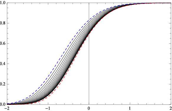
In this paper we consider the situation where at time t=0t=0 particles occupy the whole 2​ℤ2\mathbb{Z}, particles starting from 2​ℤ−2\mathbb{Z}_{-} have unit jump rate and the ones starting from 2​ℤ+2\mathbb{Z}_{+} have jump rate α\alpha. We consider large time tt and the critical scaling α−1=𝒪(t−1/3)\alpha-1={\cal O}(t^{-1/3}). In this situation the pieces of information from the two characteristics are strongly correlated and, at the same time, the system differs from the constant density case. Therefore we call this a critical scaling. We obtain the limiting process describing the fluctuations of the particles positions around the shock (see Theorem 2.2). We then perform a numerical study of the convergence of the distribution function to the one expected in the case of a shock with density jump of order one obtained in [18]. For the numerical evaluation we use the Matlab program developed by Bornemann [5] and we see that the convergence is surprisingly fast, see Figure 1.

As discussed in Section 2.3, a similar critical scaling, where particles starts from ℤ−\mathbb{Z}_{-} but the first nn particles have jump rate α\alpha has been considered in the context of last passage percolation. In the large time tt limit, the distribution function of a particle that is around the origin at time tt has a BBP distribution function [1, 11].

The rest of the paper is organized as follows. In Section 2 we define the model, discuss the macroscopic behavior, provide the main result, and finally present the numerical results. We also present the result in terms of a last passage percolation model. In Section 3 we provide the proof of the main theorem. In the appendix we give an explicit formula in terms of Airy function of the kernel appearing in the main theorem.

Acknowledgments

P.L. Ferrari was supported by the German Research Foundation via the SFB 1060–B04 project. P. Nejjar is grateful for the support of the Bonn International Graduate School (BIGS).

2 Model and results

We consider the totally asymmetric simple exclusion process and assign to each particle a label. We denote by xn​(t)∈ℤx_{n}(t)\in\mathbb{Z} the position of particle with label nn at time tt. The dynamics is as follows: each particle independently tries to jump to its right site and the jump occurs if that site is empty. The rate with which particle nn tries to jump from xn​(t)x_{n}(t) to xn​(t)+1x_{n}(t)+1 is denoted by vnv_{n}. The dynamics preserves the order of particle and we use the convention to label from right to left, i.e., xn​(t)>xn+1​(t)x_{n}(t)>x_{n+1}(t) for any n∈ℤn\in\mathbb{Z} and time tt. The process is well-defined since in a finite time no information is coming from ±∞\pm\infty (as one can see either from the graphical construction [22] or from the general Hille-Yoshida semigroup approach for interacting particle systems, see Section I.3-4 of [24]).

In this paper we consider the following specialization of the model:

xn​(0)=−2​n,n∈ℤ,vn={1,n>0,α,n≤0.\displaystyle x_{n}(0)=-2n,n\in\mathbb{Z},\quad v_{n}=\left\{\begin{array}[]{ll}1,&n>0,\\ \alpha,&n\leq 0.\end{array}\right.

As there are two jump rates involved, we call this model two-speed TASEP. Further, we call particles with label n≤0n\leq 0 α\alpha-particles and the ones with label n>0n>0 are called normal particles. We will be interested in the fluctuations of particle positions of normal particles which are around the shock created by the α\alpha-particles. First we discuss the macroscopic picture.

2.1 Macroscopic behavior

In the main result we describe the fluctuations with respect to the deterministic macroscopic behavior, given as follows. Under hydrodynamic scaling, the evolution of the particle density ϱ\varrho of the normal particles is governed by the Burgers equation

∂tϱ+∂xϱ⁡(1−ϱ)=0.\partial_{t}\varrho+\partial_{x}\varrho(1-\varrho)=0. (2.3)

The first normal particle is, however blocked by the last α\alpha-particle, which starts at the origin and moves with an average speed α/2\alpha/2. Therefore, the macroscopic density profile of the normal particles can be obtained by solving (2.3) for x∈(−∞,tα/2]x\in(-\infty,t\alpha/2] under the boundary condition ϱ⁡(t​α/2,t)=min⁡{α/2,1}\varrho(t\alpha/2,t)=\min\{\alpha/2,1\}. The system we consider corresponds to the initial condition ϱ⁡(x,0)=1/2\varrho(x,0)=1/2 for x≤0x\leq 0 and the macroscopic density profile of the normal particles is as follows: for α≥1\alpha\geq 1, there is a rarefaction fan given by

ϱ⁡(ξ​t,t)={1/2,for ​ξ≤0,(1−ξ)/2,for ​ξ∈[0,min⁡{1,α−1}],max⁡{0,1−α/2},for ​ξ∈[min⁡{1,α−1},α/2],\varrho(\xi t,t)=\left\{\begin{array}[]{ll}1/2,&\textrm{for }\xi\leq 0,\\ (1-\xi)/2,&\textrm{for }\xi\in[0,\min\{1,\alpha-1\}],\\ \max\{0,1-\alpha/2\},&\textrm{for }\xi\in[\min\{1,\alpha-1\},\alpha/2],\end{array}\right. (2.4)

while for α∈[0,1)\alpha\in[0,1) there is a shock moving with speed (α−1)/2(\alpha-1)/2,

ϱ⁡(ξ​t,t)={1/2,for ​ξ≤(α−1)/2,1−α/2,for ​ξ∈[(α−1)/2,α/2].\varrho(\xi t,t)=\left\{\begin{array}[]{ll}1/2,&\textrm{for }\xi\leq(\alpha-1)/2,\\ 1-\alpha/2,&\textrm{for }\xi\in[(\alpha-1)/2,\alpha/2].\end{array}\right. (2.5)

As a consequence, the particle with label n=⌊η​t⌋n=\lfloor\eta t\rfloor will be around the shock position if η≃(2−α)/4\eta\simeq(2-\alpha)/4.

2.2 Critical scaling regime

In this paper we focus at the critical regime where the discontinuity of the density is small. For a fixed a∈ℝa\in\mathbb{R} and a large observation time t≫1t\gg 1, we scale the jump rate of the α\alpha-particles critically, i.e., we consider

α=1−2a(t/2)−1/3.\alpha=1-2a(t/2)^{-1/3}. (2.6)

In view of the macroscopic description, particles with number given by (2−α)​t/4=t/4+a​(t/2)2/3(2-\alpha)t/4=t/4+a(t/2)^{2/3} is around the shock and its position is around −2​n+t/2=−2​a​(t/2)2/3-2n+t/2=-2a(t/2)^{2/3}. Unlike in the macroscopic shock studied in [18], where around the shock position particles are correlated over a t1/3t^{1/3} scale, in the present situation particles are correlated over a t2/3t^{2/3} scale. Therefore we consider the scaling11 1 In what follows we will not write the integer parts explicitly.

n⁡(u,t)=⌊t4+(a+u)​(t/2)2/3⌋,x⁡(u,t)=⌊−2​(a+u)​(t/2)2/3⌋,n(u,t)=\left\lfloor\frac{t}{4}+(a+u)(t/2)^{2/3}\right\rfloor,\quad x(u,t)=\left\lfloor-2(a+u)(t/2)^{2/3}\right\rfloor, (2.7)

and define the accordingly scaled particle position process by

u↦Xt​(u)=xn⁡(u,t)−x⁡(u,t)−(t/2)1/3.u\mapsto X_{t}(u)=\frac{x_{n(u,t)}-x(u,t)}{-(t/2)^{1/3}}. (2.8)

Our main analytic result is the limit process ℳa=limt→∞Xt{\cal M}_{a}=\lim_{t\to\infty}X_{t}.

Definition 2.1 (The limit process ℳa\mathcal{M}_{a}).

Define the extended kernel

Ka​(u1,ξ1,u2,ξ2)=−14​π​(u2−u1)​exp⁡(−(ξ2−ξ1)24​(u2−u1))​𝟙​(u2>u1)\displaystyle K_{a}(u_{1},\xi_{1};u_{2},\xi_{2})=-\frac{1}{\sqrt{4\pi(u_{2}-u_{1})}}\exp\left(-\frac{(\xi_{2}-\xi_{1})^{2}}{4(u_{2}-u_{1})}\right)\mathbbm{1}(u_{2}>u_{1}) (2.9)
+−1(2​π​i)2∫γ+dw∫γ−dzew3/3+(u2+a)​w2−ξ2​wez3/3+(u1+a)​z2−ξ1​z2​w(z−w)​(z+w)\displaystyle+\frac{-1}{(2\pi\mathrm{i})^{2}}\int_{\gamma_{+}}\mathrm{d}w\int_{\gamma_{-}}\mathrm{d}z\frac{e^{w^{3}/3+(u_{2}+a)w^{2}-\xi_{2}w}}{e^{z^{3}/3+(u_{1}+a)z^{2}-\xi_{1}z}}\frac{2w}{(z-w)(z+w)}
+1(2​π​i)2∫Γ+dw∫Γ−dzew3/3+(u2−a)​w2−w⁡(ξ2+4​a​u2)+4​u2​a2ez3/3+(u1−a)​z2−z⁡(ξ1+4​a​u1)+4​u1​a22​(w−2​a)(z+w)​(z−w+4​a).\displaystyle+\frac{1}{(2\pi\mathrm{i})^{2}}\int_{\Gamma_{+}}\mathrm{d}w\int_{\Gamma_{-}}\mathrm{d}z\frac{e^{w^{3}/3+(u_{2}-a)w^{2}-w(\xi_{2}+4au_{2})+4u_{2}a^{2}}}{e^{z^{3}/3+(u_{1}-a)z^{2}-z(\xi_{1}+4au_{1})+4u_{1}a^{2}}}\frac{2(w-2a)}{(z+w)(z-w+4a)}.

The curves can be chosen as follows. Let θ=max⁡{|u1|+|a|,|u2|+|a|}\theta=\max\{|u_{1}|+|a|,|u_{2}|+|a|\}. For any choice of r±,R±r_{\pm},R_{\pm} satisfying r+>−r−>θr_{+}>-r_{-}>\theta and −R−>R+>θ+4​|a|-R_{-}>R_{+}>\theta+4|a|, we can set γ±=r±+i​ℝ\gamma_{\pm}=r_{\pm}+\mathrm{i}\mathbb{R} and Γ±=R±+i​ℝ\Gamma_{\pm}=R_{\pm}+\mathrm{i}\mathbb{R} (oriented with increasing imaginary parts). The limit process ℳa\mathcal{M}_{a} is defined by its finite-dimensional distribution: for any given u1<u2<⋯<umu_{1}<u_{2}<\cdots<u_{m},

ℙ(⋂k=1m{ℳa(uk)≤sk})=det(𝟙−χsKaχs)L2​({u1,…,um}×ℝ)\mathbb{P}\left(\bigcap_{k=1}^{m}\{\mathcal{M}_{a}(u_{k})\leq s_{k}\}\right)=\det(\mathbbm{1}-\chi_{s}K_{a}\chi_{s})_{L^{2}(\{u_{1},\ldots,u_{m}\}\times\mathbb{R})} (2.10)

where χs​(uk,x)=𝟙​(x>sk)\chi_{s}(u_{k},x)=\mathbbm{1}(x>s_{k}). An explicit expression of KaK_{a} in terms of Airy functions is given in Appendix A.

With this definition we can state our main analytic result, proven in Section 3.

Theorem 2.2.

It holds

limt→∞Xt​(u)=ℳa​(u)\lim_{t\to\infty}X_{t}(u)=\mathcal{M}_{a}(u) (2.11)

in the sense of finite dimensional distributions.

Remark 2.3.

In some special cases or limits we recover previous known processes. For example:

  • (a)

    For a=0a=0 we have the flat TASEP and see the Airy1 process [8, 27]: ℳ0(u)=21/3𝒜1(2−2/3u){\cal M}_{0}(u)=2^{1/3}{\cal A}_{1}(2^{-2/3}u).

  • (b)

    When a→−∞a\to-\infty a rarefaction fan is created. At his left edge, ℳa{\cal M}_{a} becomes the Airy2→1 process [9]: lima→−∞ℳa​(u−a)=𝒜2→1​(u)\lim_{a\to-\infty}{\cal M}_{a}(u-a)={\cal A}_{2\to 1}(u). Inside the rarefaction fan ℳa{\cal M}_{a} becomes the Airy2 process [26]. For instance, in the middle of the rarefaction fan: lima→−∞ℳa​(u)+(u+a)2=𝒜2​(u)\lim_{a\to-\infty}{\cal M}_{a}(u)+(u+a)^{2}={\cal A}_{2}(u).

  • (c)

    For a>0a>0, there is a shock and ℳa{\cal M}_{a} is a transition process between two 𝒜1{\cal A}_{1} processes. Indeed, limM→∞ℳa(u±M)=21/3𝒜1(2−2/3u)\lim_{M\to\infty}{\cal M}_{a}(u\pm M)=2^{1/3}{\cal A}_{1}(2^{-2/3}u).

Further, when a→∞a\to\infty one should recover the macroscopic shock picture and by the result of [18] the one-point distribution should become a product of two F1F_{1} distributions, where F1F_{1} is the GOE Tracy-Widom distribution discovered first in random matrix theory [28]. More precisely, extrapolating the result of Corollary 2.5 in [18] (reported below for convenience) we conjecture that

lima→∞ℙ⁡(ℳa​(0)≤s)=(F1​(22/3​s))2.\lim_{a\to\infty}\mathbb{P}({\cal M}_{a}(0)\leq s)=(F_{1}(2^{2/3}s))^{2}. (2.12)

As the kernel KaK_{a} is not converging pointwise as a→∞a\to\infty (not even after an appropriate conjugation) we could not verify the conjecture analytically. The numerical studies presented in Section 2.4 below are in agreement with the conjecture and, moreover, show that the convergence as aa increases is quite fast.

Theorem 2.4 (Corollary 2.5 in [18]).

Let xn​(0)=−2​nx_{n}(0)=-2n for n∈ℤn\in\mathbb{Z}. For α<1\alpha<1 let η=2−α4\eta=\frac{2-\alpha}{4} and v=−1−α2v=-\frac{1-\alpha}{2}. Then it holds

limt→∞ℙ⁡(xη​t​(t)≥v​t−s​t1/3)=F1​(2​s)​F1​(2​s​σα),\lim_{t\to\infty}\mathbb{P}\left(x_{\eta t}(t)\geq vt-st^{1/3}\right)=F_{1}\left(2s\right)F_{1}\left(2s\sigma_{\alpha}\right), (2.13)

with σα=α1/3​(2−2​α+α2)1/3(2−α)2/3\sigma_{\alpha}=\frac{\alpha^{1/3}(2-2\alpha+\alpha^{2})^{1/3}}{(2-\alpha)^{2/3}}. Note that σα→1\sigma_{\alpha}\to 1 as α→1\alpha\to 1.

2.3 Last passage percolation

The limit process ℳa{\cal M}_{a} occurs in a related last passage percolation (LPP) model as well. To each site (i,j)(i,j) of ℤ2\mathbb{Z}^{2} we assign an independent random variable ω(i,j)\omega_{(i,j)} with

ω(i,j)∼exp⁡(vj).\omega_{(i,j)}\sim\exp(v_{j}). (2.14)

Further, to a TASEP initial condition {xn​(0),n∈ℤ}\{x_{n}(0),n\in\mathbb{Z}\} we assign the line

ℒ={(n+xn​(0),n)|n∈ℤ}.{\cal L}=\{(n+x_{n}(0),n)\,|\,n\in\mathbb{Z}\}. (2.15)

For a point (m,n)(m,n) on the right/above the line ℒ\cal L, the last passage time from ℒ{\cal L} to (m,n)(m,n) is defined by

Lℒ→(m,n):=maxπ:ℒ→(m,n)∑(i,j)∈πω(i,j),L_{{\cal L}\to(m,n)}:=\max_{\pi:{\cal L}\to(m,n)}\sum_{(i,j)\in\pi}\omega_{(i,j)}, (2.16)

where the maximum is taken over all up-right paths22 2 An up-right path π={π⁡(0),…,π⁡(n)}\pi=\{\pi(0),\ldots,\pi(n)\} is a sequence of points of ℤ2\mathbb{Z}^{2} such that π⁡(i+1)−π⁡(i)∈{(1,0),(0,1)}\pi(i+1)-\pi(i)\in\{(1,0),(0,1)\}, for i=0,…,n−1i=0,\ldots,n-1. from ℒ\cal L to (m,n)(m,n). The well-known connection between TASEP and LPP is

ℙ(⋂k=1r{xnk(t)≥mk−nk})=ℙ(⋂k=1r{Lℒ→(mk,nk)≤t}).\mathbb{P}\bigg(\bigcap_{k=1}^{r}\{x_{n_{k}}(t)\geq m_{k}-n_{k}\}\bigg)=\mathbb{P}\bigg(\bigcap_{k=1}^{r}\{L_{{\cal L}\to(m_{k},n_{k})}\leq t\}\bigg). (2.17)

In our model, we have ℒ={(−n,n),n∈ℤ}{\cal L}=\{(-n,n),n\in\mathbb{Z}\}. Consider the critical scaling

α=1−2a(2ℓ)−1/3,\alpha=1-2a(2\ell)^{-1/3}, (2.18)

and focus at the position

m⁡(v,ℓ)=ℓ−2​(v+a)​(2​ℓ)2/3,n=ℓ.m(v,\ell)=\ell-2(v+a)(2\ell)^{2/3},\quad n=\ell. (2.19)

Define the rescaled LPP time by

Lℓresc​(v):=Lℒ→(m⁡(v,ℓ),ℓ)−[4​ℓ−4​(v+a)​(2​ℓ)2/3]2​(2​ℓ)1/3.L^{\rm resc}_{\ell}(v):=\frac{L_{{\cal L}\to(m(v,\ell),\ell)}-\left[4\ell-4(v+a)(2\ell)^{2/3}\right]}{2(2\ell)^{1/3}}. (2.20)
Theorem 2.5.

It holds

limℓ→∞Lℓresc​(v)=ℳa​(v)\lim_{\ell\to\infty}L^{\rm resc}_{\ell}(v)=\mathcal{M}_{a}(v) (2.21)

in the sense of finite dimensional distributions.

In short, to prove Theorem 2.5, one starts with the relation (2.17) that gives the joint distributions of LℓrescL^{\rm resc}_{\ell} in terms of positions of TASEP particles at different times, varying around t=4​ℓt=4\ell on a ℓ2/3\ell^{2/3} scale only. By the slow-decorrelation phenomenon [17, 13] the fluctuations at different times are asymptotically the same as the fixed time fluctuations for points lying on special space-time directions (the characteristics). At fixed time, the result is exactly given by Theorem 2.2. The details of this procedure have been worked out for instance in [2, 12].

2.4 Numerical study

Here we numerically compute the distribution function of the process ℳa{\cal M}_{a}, given by a Fredholm determiant of the kernel KaK_{a}, as well as some of its basic statistics: Expectation, Variance, Skewness, Kurtosis. For the computation, we use the formula for KaK_{a} given in the Appendix A, since Airy functions are already implemented functions in Matlab, and apply Bornemann’s method for the evaluation of the Fredholm determinants, see [14], which is well-adapted for analytic kernels. Bornemann’s algorithm also comes with an error control that we used, see Section 4.4 of [14].
Refer to caption
Figure 1: The dashed lines are s↦F1​(2​s)s\mapsto F_{1}(2s) (the left one) and s↦F1​(2​s)2s\mapsto F_{1}(2s)^{2} (the right one), s∈[−2,2]s\in[-2,2]. The solid lines are the functions s↦Ga​(s)s\mapsto G_{a}(s) for a=0.1,0.2,…,1.8a=0.1,0.2,\ldots,1.8. For a=0a=0, G0​(s)=F1​(2​s)G_{0}(s)=F_{1}(2s), when aa grows larger, Ga​(s)G_{a}(s) approximates the macroscopic shock distribution F1​(2​s)2F_{1}(2s)^{2} as conjectured, see (2.22).

For simplicity, we study the validity of the conjecture in (2.12), i.e., we set u=0u=0. In principle, one could look also general uu, but then it has to be taken as a function of aa too (since in the unscaled process the correlation scale of the process changes from t2/3t^{2/3} to t1/3t^{1/3} as α\alpha varies from 11 to a value strictly less then 11).

To avoid to carry around a lot of 21/32^{1/3} factors, we rescale space by a factor 21/32^{1/3} so that the conjecture (2.12) writes

lima→∞ℙ⁡(ℳa​(0)≤s​21/3)=(F1​(2​s))2.\lim_{a\to\infty}\mathbb{P}({\cal M}_{a}(0)\leq s2^{1/3})=(F_{1}(2s))^{2}. (2.22)

We denote K~a​(ξ1,ξ2):=21/3​Ka​(0,21/3​ξ1,0,21/3​ξ2)\widetilde{K}_{a}(\xi_{1},\xi_{2}):=2^{1/3}K_{a}(0,2^{1/3}\xi_{1};0,2^{1/3}\xi_{2}). Remark that the special case a=0a=0 we have the Airy1 kernel, K~0​(ξ1,ξ2)=Ai⁡(ξ1+ξ2)\widetilde{K}_{0}(\xi_{1},\xi_{2})=\mathrm{Ai}(\xi_{1}+\xi_{2}). By (2.10) we have

Ga​(s):=ℙ⁡(ℳa​(0)≤s​21/3)=det(𝟙−χsc​K~a​χsc),χsc=𝟙(s,∞).\displaystyle G_{a}(s):=\mathbb{P}({\cal M}_{a}(0)\leq s2^{1/3})=\det(\mathbbm{1}-\chi_{s}^{c}\widetilde{K}_{a}\chi_{s}^{c}),\quad\chi_{s}^{c}=\mathbbm{1}_{(s,\infty)}. (2.23)

By Theorem 2.2, this is the t→∞t\to\infty limit of the rescaled position of a particle in the microscopic shock. As mentioned earlier, we let aa grow large so as to recover the macroscopic shock distribution, which for large but finite time tt would correspond to the choice a=(1−α)​t1/324/3a=\frac{(1-\alpha)t^{1/3}}{2^{4/3}}. Due to the numerical limitations discussed below, we will compute GaG_{a} and its basic statistics up to a=1.8a=1.8. Surprisingly, already for this relatively small value of aa, one is already quite close to the asymptotic behavior. The reason for this is the following. At first approximation, from the KPZ scalings, we know that the randomness that influences the statistical properties of particle positions around the shock lives in a t2/3t^{2/3} neighborhood of the characteristic lines that comes together at the shock (for a proof in a special case, see [23]) and the neighborhood should be quite tight to provide the super-exponential decay of the covariance for the Airy1 process [6]. Further, by a closer inspection near the end-points, we discover that at t1/3t^{1/3} distance from the shock, the neighborhood is only of order t1/3t^{1/3} as well [18, 19]. These two phenomena imply that the convergence will happen on aa of order 11.

Numerical Limitations

The limitation to a≤1.8a\leq 1.8 is due to the numerical difficulty of evaluating GaG_{a} for aa large. As aa grows, K~a\widetilde{K}_{a} has some terms which are of order 11 and one term which is (super-) exponentially diverging. More precisely, one has

(A.4)=e4​a3/3−2​a​(ξ1+ξ2)−(ξ2−ξ1)2/16​a−ln⁡(4​π​a)+ε0​(a)(A.3)=2−1/3Ai(2−1/3(ξ1+ξ2))e−a⁡(ξ2−ξ1)+ε1(a)(A.5)=2−1/3Ai(2−1/3(ξ1+ξ2))e−a⁡(ξ1−ξ2)+ε2(a)|(A.2)|≤cimaxλ≥0Ai(λ+ξi+a2),i=1,2.,\begin{aligned} &\eqref{divstrong}=e^{4a^{3}/3-2a(\xi_{1}+\xi_{2})-(\xi_{2}-\xi_{1})^{2}/16a-\ln(4\sqrt{\pi a})}+\varepsilon_{0}(a)\\ &\eqref{div1}=2^{-1/3}\mathrm{Ai}(2^{-1/3}(\xi_{1}+\xi_{2}))e^{-a(\xi_{2}-\xi_{1})}+\varepsilon_{1}(a)\\ &\eqref{div2}=2^{-1/3}\mathrm{Ai}(2^{-1/3}(\xi_{1}+\xi_{2}))e^{-a(\xi_{1}-\xi_{2})}+\varepsilon_{2}(a)\\ &\left|\eqref{vanishing}\right|\leq c_{i}\max_{\lambda\geq 0}\mathrm{Ai}(\lambda+\xi_{i}+a^{2}),\quad i=1,2.\end{aligned}, (2.24)

where |ε0​(a)|≤1/4​a|\varepsilon_{0}(a)|\leq 1/4a, and, for i=1,2i=1,2, |εi​(a)|≤maxλ≥0⁡Ai⁡(λ+ξi+a2)/a|\varepsilon_{i}(a)|\leq\max_{\lambda\geq 0}\mathrm{Ai}(\lambda+\xi_{i}+a^{2})/a and ci=∫0∞d​λ​Ai​(ξ3−i+a2+λ)c_{i}=\int_{0}^{\infty}\mathrm{d}\lambda\mathrm{Ai}(\xi_{3-i}+a^{2}+\lambda). This implies that when aa increases, the ratio between the bounded terms and the large term becomes smaller than 10−1610^{-16} machine precision and no reliable numerical evaluation is possible. In our case, already for a≥4a\geq 4, K~a\widetilde{K}_{a} (much less GaG_{a}) can no longer be computed in Matlab. For instance, Matlab computes G3​(s)=NaNG_{3}(s)={\rm NaN} for all tested ss, G2.5​(−1)=0.0838G_{2.5}(-1)=0.0838 with an error 0.00440.0044, whereas G1.8​(−2)=1.4879⋅10−4G_{1.8}(-2)=1.4879\cdot 10^{-4}, with an error 5.6831⋅10−95.6831\cdot 10^{-9}. We present the numerical computations until a=1.8a=1.8, since for higher values the error term in the Kurtosis becomes visible.

Generally, the computational error of Ga​(s)G_{a}(s) decreases as ss increases since then K~a​(ξ1,ξ2)\widetilde{K}_{a}(\xi_{1},\xi_{2}) needs to be computed only for small entries and the evaluation of GaG_{a} is easier (namely, the matrix whose determinant approximates GaG_{a} gets closer to the Identity matrix as ss increases, see (4.3) in [14]). The statistics of GaG_{a} were computed using the chebfun package (see [3]), in which GaG_{a} is represented by its polynomial interpolant in Chebyshev points, for our choice in n=4096n=4096 points.

In Figure 1 we plot F1​(2​s)=G0​(s)F_{1}(2s)=G_{0}(s), Ga​(s)G_{a}(s) for a∈{0.1,0.2,…,1.8}a\in\{0.1,0.2,\ldots,1.8\} and the conjectured a→∞a\to\infty limit, namely (F1​(2​s))2(F_{1}(2s))^{2}. A property which is apparent from Figure 1 is that GaG_{a} monotonically decreases towards F1​(2​s)2F_{1}(2s)^{2} as aa grows. Indeed, for all a,a′∈{0,…,1.8}a,a^{\prime}\in\{0,\ldots,1.8\}, and s∈{−2,−1.9,…,2}s\in\{-2,-1.9,\ldots,2\} we have

Ga(s)>F1(2s)2,Ga′(s)<Ga(s)ifa<a′.G_{a}(s)>F_{1}(2s)^{2},\quad G_{a^{\prime}}(s)<G_{a}(s)\quad{\rm if}\quad a<a^{\prime}. (2.25)

An analytic proof of this property does not seem to be trivial and is not available so far.

To further quantify the difference between F1.8F_{1.8} and F1(2⋅)2F_{1}(2\cdot)^{2} we computed

D⁡(a):=maxs=−2,−1.9,…,2⁡|F1​(2​s)2−G1.8​(s)|.D(a):=\max_{s=-2,-1.9,\ldots,2}|F_{1}(2s)^{2}-G_{1.8}(s)|. (2.26)
Refer to caption
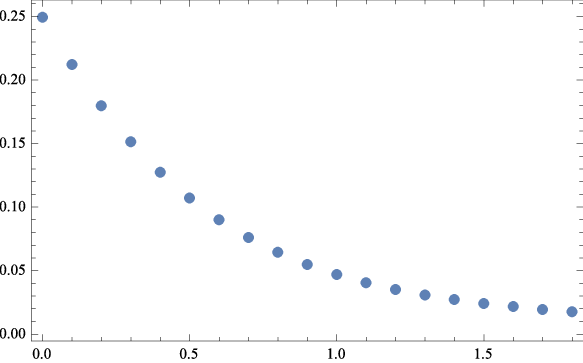
Figure 2: Plot of the function a↦D⁡(a)a\mapsto D(a) defined by (2.26). On this limited interval width for aa the convergence of the difference of the distribution functions close to exponentially fast.

(2.25) and (2.26) are compatible with the conjecture (2.22), but to have a further more reliable verification we study numerically the basis statistics too. The reason is that the distribution functions might be optically close but still be different. For example, the plots of the GUE and GOE Tracy-Widom distribution functions scaled to have both average 00 and variance 11, are almost indistinguishable. However, by looking at their skewness and kurtosis one can clearly differentiate between them.

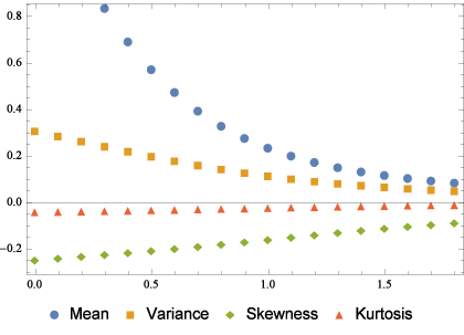
In Figure 3 we plot the basic statistics of GaG_{a} and compare them with those of F1(2⋅)2F_{1}(2\,\cdot)^{2}. The approximation is fastest for the expectation, and slowest for the kurtosis (though the observation window for aa is too small to quantify the different rates of convergence).
Refer to caption
Figure 3: Relative difference between the basic statistics of GaG_{a} and of the conjectured limiting distribution, F1(2⋅)2F_{1}(2\cdot)^{2}.

Finally, let us resume in Table 1 the basic statistics of GaG_{a} in comparison to F1(2⋅)2F_{1}(2\cdot)^{2}.

Expectation Variance Skewness Kurtosis
G0G_{0} −0.6033;144%-0.6033;144\% 0.4019;31%0.4019;31\% 0.2935;−25%0.2935;-25\% 3.1652;−4.3%3.1652;-4.3\%
G0.3G_{0.3} −0.4524;83%-0.4524;83\% 0.3816;24%0.3816;24\% 0.3028;−23%0.3028;-23\% 3.1811;−3.9%3.1811;-3.9\%
G0.6G_{0.6} −0.3632;47%-0.3632;47\% 0.3624;17%0.3624;17\% 0.3127;−20%0.3127;-20\% 3.1988;−3.3%3.1988;-3.3\%
G0.9G_{0.9} −0.3145;27%-0.3145;27\% 0.3466;13%0.3466;13\% 0.3240;−17%0.3240;-17\% 3.2184;−2.7%3.2184;-2.7\%
G1.2G_{1.2} −0.2889;17%-0.2889;17\% 0.3353;8.9%0.3353;8.9\% 0.3359;−14%0.3359;-14\% 3.2377;−2.1%3.2377;-2.1\%
G1.5G_{1.5} −0.2751;11%-0.2751;11\% 0.3277;6.4%0.3277;6.4\% 0.3469;−11%0.3469;-11\% 3.2540;−1.6%3.2540;-1.6\%
G1.8G_{1.8} −0.2670;8.2%-0.2670;8.2\% 0.3226;4.7%0.3226;4.7\% 0.3561;−9.1%0.3561;-9.1\% 3.2658;−1.3%3.2658;-1.3\%
𝑭𝟏(𝟐⋅)𝟐\boldsymbol{F_{1}(2\cdot)^{2}} −0.2468-0.2468 0.30800.3080 0.39170.3917 3.30863.3086
Table 1: Data of the basic statistics and their relative difference to the conjectured limit distribution F1(2⋅)2F_{1}(2\,\cdot)^{2} for a few values of aa.

3 Asymptotic analysis - Proof of Theorem 2.2

In Section 3.1 we derive the finite time kernel, whose Fredholm determinant gives us the joint distributions of TASEP particle positions, see Proposition 3.1. For the derivation we first need to consider the case of a finite number MM of α\alpha-particles and then take the M→∞M\to\infty limit. In Section 3.2 we then perform the asymptotic analysis and complete the proof of Theorem 2.2.

3.1 Finite time formula

Taking the limit of the situation with finitely many slow particles we obtain the following result.

Proposition 3.1.

Consider Two-Speed TASEP as defined in (2). Then the joint distribution of the positions of mm normal particles with labels 0<n1<n2<…<nm0<n_{1}<n_{2}<\ldots<n_{m} at time tt is given by

ℙ(⋂k=1m{xnk(t)>sk})=det(1−χsKχs)ℓ2​({n1,…,nm}×ℤ),\mathbb{P}\left(\bigcap_{k=1}^{m}\{x_{n_{k}}(t)>s_{k}\}\right)=\det(1-\chi_{s}K\chi_{s})_{\ell^{2}(\{n_{1},\ldots,n_{m}\}\times\mathbb{Z})}, (3.1)

with K=−ϕ+K1+K2K=-\phi+K^{1}+K^{2}, where χs(nk,x)=𝟙(−∞,sk](x)\chi_{s}(n_{k},x)=\mathbbm{1}_{(-\infty,s_{k}]}(x) and33 3 For a set SS, the notation ΓS\Gamma_{S} means a simple path anticlockwise oriented enclosing only poles of the integrand belonging to the set SS.

ϕ(n1,x1;n2,x2)=12​π​i∮Γ0d​ww(w−1)n1−n2wx1−x2+n1−n2𝟙{n1<n2},\phi(n_{1},x_{1};n_{2},x_{2})=\frac{1}{2\pi\mathrm{i}}\oint_{\Gamma_{0}}\frac{\mathrm{d}w}{w}\frac{(w-1)^{n_{1}-n_{2}}}{w^{x_{1}-x_{2}+n_{1}-n_{2}}}\mathbbm{1}_{\{n_{1}<n_{2}\}}, (3.2)
K1​(n1,x1,n2,x2)=\displaystyle K^{1}(n_{1},x_{1};n_{2},x_{2})= 1(2​π​i)2​∮Γ0d​v​∮Γ0,−vd​ww​et​w​(w−1)n1wx1+n1\displaystyle\frac{1}{(2\pi\mathrm{i})^{2}}\oint_{\Gamma_{0}}\mathrm{d}v\oint_{\Gamma_{0,-v}}\frac{\mathrm{d}w}{w}\frac{e^{tw}(w-1)^{n_{1}}}{w^{x_{1}+n_{1}}} (3.3)
×(1+v)x2+n2et⁡(v+1)​vn2​1+2​v(w+v)​(w−v−1),\displaystyle\times\frac{(1+v)^{x_{2}+n_{2}}}{e^{t(v+1)}v^{n_{2}}}\frac{1+2v}{(w+v)(w-v-1)},

and

K2​(n1,x1,n2,x2)=\displaystyle K^{2}(n_{1},x_{1};n_{2},x_{2})= −1(2​π​i)2​∮Γ0d​w​∮Γ0,α−1−wd​v​et​w​(w−1)n1wx1+n1+1​(1+v)x2+n2et⁡(v+1)​vn2\displaystyle\frac{-1}{(2\pi\mathrm{i})^{2}}\oint_{\Gamma_{0}}\mathrm{d}w\oint_{\Gamma_{0,\alpha-1-w}}\mathrm{d}v\frac{e^{tw}(w-1)^{n_{1}}}{w^{x_{1}+n_{1}+1}}\frac{(1+v)^{x_{2}+n_{2}}}{e^{t(v+1)}v^{n_{2}}} (3.4)
×1+2​v(v+w+1−α)​(w−v−α).\displaystyle\times\frac{1+2v}{(v+w+1-\alpha)(w-v-\alpha)}.

The system with finitely many slow particles has been already partially studied in [10]. There, it was shown that the distribution function of particles positions is given by a Fredholm determinant and the kernel was given. For a fixed M∈ℕM\in\mathbb{N}, consider TASEP with initial conditions and jump rates given by

xnM​(0)=2​(M−n),n∈ℕ,vnM={1,for ​n>M,α,for ​1≤n≤M.\displaystyle x_{n}^{M}(0)=2(M-n),\quad n\in\mathbb{N},\qquad v_{n}^{M}=\left\{\begin{array}[]{ll}1,&\textrm{for }n>M,\\ \alpha,&\textrm{for }1\leq n\leq M.\end{array}\right.

To distinguish this system with the one we want to study, i.e., M=∞M=\infty, we will index all quantities by a MM. Proposition 6 of [10] tells us that

ℙ(⋂k=1m{xnk+MM(t)>sk})=det(1−χsKMχs)ℓ2​({n1,…,nm}×ℤ),\mathbb{P}\left(\bigcap_{k=1}^{m}\{x_{n_{k}+M}^{M}(t)>s_{k}\}\right)=\det(1-\chi_{s}K^{M}\chi_{s})_{\ell^{2}(\{n_{1},\ldots,n_{m}\}\times\mathbb{Z})}, (3.7)

where the kernel kernel KMK^{M} has the decomposition

KM=−ϕ+K1+K2,M.\displaystyle K^{M}=-\phi+K^{1}+K^{2,M}. (3.8)

Here ϕ\phi and K1K^{1} are as in Proposition 3.1, while K2,MK^{2,M} is given by

K2,M​(n1,x1,n2,x2)=\displaystyle K^{2,M}(n_{1},x_{1};n_{2},x_{2})= 1(2​π​i)3​∮Γα−1d​v​∮Γ0,vd​z​∮Γ0,α−1−vd​ww​et​w​(w−1)n1wx1+n1\displaystyle\frac{1}{(2\pi\mathrm{i})^{3}}\oint_{\Gamma_{\alpha-1}}\mathrm{d}v\oint_{\Gamma_{0,v}}\mathrm{d}z\oint_{\Gamma_{0,\alpha-1-v}}\frac{\mathrm{d}w}{w}\frac{e^{tw}(w-1)^{n_{1}}}{w^{x_{1}+n_{1}}} (3.9)
×(1+z)x2+n2et​z​zn2​(w⁡(w−α)(v+1)​(v+1−α))M\displaystyle\times\frac{(1+z)^{x_{2}+n_{2}}}{e^{tz}z^{n_{2}}}\left(\frac{w(w-\alpha)}{(v+1)(v+1-\alpha)}\right)^{M}
×(1+2​z)​(2​v+2−α)(z−v)​(z+v+1)​(w−1−v)​(w+1−α+v).\displaystyle\times\frac{(1+2z)(2v+2-\alpha)}{(z-v)(z+v+1)(w-1-v)(w+1-\alpha+v)}.
Proof of Proposition 3.1.

First we note that

limM→∞ℙ(⋂k=1m{xnk+MM(t)>s})=ℙ(⋂k=1m{xnk(t)>s}).\lim_{M\to\infty}\mathbb{P}\left(\bigcap_{k=1}^{m}\{x_{n_{k}+M}^{M}(t)>s\}\right)=\mathbb{P}\left(\bigcap_{k=1}^{m}\{x_{n_{k}}(t)>s\}\right). (3.10)

This follows since xn+MM​(0)=xn​(0)x_{n+M}^{M}(0)=x_{n}(0) for all n≥−Mn\geq-M and by the fact that in TASEP the positions of the normal particles up to a fixed time tt depend only on finitely many other particles on the right with probability one, as is seen from a graphical construction of it. So it remains to show that the convergence in (3.11) holds also on the level of fredholm determinants.

First of all, as shown already in Corollary 8 of [10]), it holds

limM→∞KM​(n1+M,x1,n2+M,x2)=K⁡(n1,x1,n2,x2)\lim_{M\to\infty}K^{M}(n_{1}+M,x_{1};n_{2}+M,x_{2})=K(n_{1},x_{1};n_{2},x_{2}) (3.11)

pointwise. The reason being that for any M>(n1+x1+1)M>(n_{1}+x_{1}+1) the pole at w=0w=0 in (3.9) vanishes, in the limit of large MM we can integrate out explicitly the simple pole at w=α−1−vw=\alpha-1-v of the kernel K2,MK^{2,M} and it results in the kernel K2K^{2} given in Proposition 3.1.

To show the convergence of Fredholm determinants we use their series expansion expression, namely

det(𝟙−χs​KM​χs)ℓ2​({n1,…,nm}×ℤ)=∑n≥0(−1)nn!​∑i1,…,in=1m∑x1≤s1…​∑xn≤sndet[KM​(nik,xk,nil,xl)]1≤k,l≤n.\det(\mathbbm{1}-\chi_{s}K^{M}\chi_{s})_{\ell^{2}(\{n_{1},\ldots,n_{m}\}\times\mathbb{Z})}\\ =\sum_{n\geq 0}\frac{(-1)^{n}}{n!}\sum_{i_{1},\ldots,i_{n}=1}^{m}\sum_{x_{1}\leq s_{1}}\ldots\sum_{x_{n}\leq s_{n}}\det[K^{M}(n_{i_{k}},x_{k};n_{i_{l}},x_{l})]_{1\leq k,l\leq n}. (3.12)

It is easy to see that K1​(n1,x1,n2,x2)=0K^{1}(n_{1},x_{1};n_{2},x_{2})=0 for x1<−2​n1x_{1}<-2n_{1} since the pole at w=0w=0 vanishes after computing the residue at w=−vw=-v the pole at v=0v=0 vanishes. Similarly, K2,M​(n1,x1,n2,x2)=0K^{2,M}(n_{1},x_{1};n_{2},x_{2})=0 for x1<−n1x_{1}<-n_{1} since the pole at w=0w=0 vanishes. Further, in the term ϕ⁡(n1,x1,n2,x2)\phi(n_{1},x_{1};n_{2},x_{2}), if x2x_{2} is bounded from below, then for x1x_{1} small enough this term is also zero. This implies that the n×nn\times n determinant in (3.12) is strictly equal to zero if xi<−2​nmx_{i}<-2n_{m}. The physical reason for this is that if we consider the system with particle numbers bounded from above by nmn_{m}, then by TASEP dynamics particles can be present only in the region on the right of xnm​(0)=−2​nmx_{n_{m}}(0)=-2n_{m}. Consequently, the sums are finite and the by Hadamard bound |det[KM​(nik,xk,nil,xl)]1≤k,l≤n|≤Cn​nn/2|\det[K^{M}(n_{i_{k}},x_{k};n_{i_{l}},x_{l})]_{1\leq k,l\leq n}|\leq C^{n}n^{n/2} for some finite constant CC. Thus by dominated convergence we can take the limit M→∞M\to\infty inside the sum and the proof is completed. ∎

3.2 Scaling limit and asymptotics

With the finite time formula of Proposition 3.1 at hand, we can now proceed to prove the main result.

Proof of Theorem 2.2.

The proof is identical to the one of Theorem 2.5 in [7], given that the we have convergence of the (properly rescaled) kernel in a bounded set (Proposition 3.2), and good enough bounds to control the convergence of the Fredholm determinant by the use of dominated convergence. The strategy, nowadays standard, was first used by Tracy, Widom and Gravner in [21]. The bounds are contained in Propositions 3.3,  3.4, and 3.5 below. ∎

From now on, the uiu_{i} are some fixed real values. We first prove convergence to the limit kernel KaK_{a} and then provide integrable bounds. We consider the scaling

ni​(u,t)\displaystyle n_{i}(u,t) =t/4+(ui+a)​(t/2)2/3,\displaystyle=t/4+(u_{i}+a)\left(t/2\right)^{2/3}, (3.13)
xi​(u,t)\displaystyle x_{i}(u,t) =−2​(ui+a)​(t/2)2/3−ξi​(t/2)1/3.\displaystyle=-2(u_{i}+a)\left(t/2\right)^{2/3}-\xi_{i}\left(t/2\right)^{1/3}.

The ξi\xi_{i} measure the fluctuations in the (t/2)1/3(t/2)^{1/3} scale with respect to the macroscopic approximation given in (2.7). Accordingly, we define the rescaled kernel

Kresc​(u1,ξ1,u2,ξ2)=2x2−x1​(−1)n1−n2​(t/2)1/3​K​(n1,x1,n2,x2)K^{{\rm resc}}(u_{1},\xi_{1};u_{2},\xi_{2})=2^{x_{2}-x_{1}}(-1)^{n_{1}-n_{2}}\left(t/2\right)^{1/3}K(n_{1},x_{1};n_{2},x_{2}) (3.14)

and similarly for each component of the kernel.

Proposition 3.2 (Convergence on bounded sets).

For any fixed L>0L>0, we have

limt→∞Kresc​(u1,ξ1,u2,ξ2)=Ka​(u1,ξ1,u2,ξ2),\displaystyle\lim_{t\to\infty}K^{\rm resc}(u_{1},\xi_{1};u_{2},\xi_{2})=K_{a}(u_{1},\xi_{1};u_{2},\xi_{2}), (3.15)

uniformly for ξ1,ξ2\xi_{1},\xi_{2} in [−L,L][-L,L]. Here KaK_{a} is the kernel from Theorem 2.2.

Proof.

We start with ϕ\phi. The residue at 00 can be easily computed expanding (w−1)n1−n2(w-1)^{n_{1}-n_{2}} with the binomial formula and one readily obtains that ϕ⁡(n1,x1,n2,x2)=(−1)n1−n2​(x1−x2−1n2−n1−1)\phi(n_{1},x_{1};n_{2},x_{2})=(-1)^{n_{1}-n_{2}}{x_{1}-x_{2}-1\choose n_{2}-n_{1}-1}. It is then an easy computation to show that (see e.g. Proposition 7 of [9])

ϕresc​(u1,ξ1,u2,ξ2)→𝟙{u2>u1}4​π​(u2−u1)​exp⁡(−(ξ2−ξ1)24​(u2−u1)).\phi^{\rm resc}(u_{1},\xi_{1};u_{2},\xi_{2})\to\frac{\mathbbm{1}_{\{u_{2}>u_{1}\}}}{\sqrt{4\pi(u_{2}-u_{1})}}\exp\left(-\frac{(\xi_{2}-\xi_{1})^{2}}{4(u_{2}-u_{1})}\right). (3.16)

Next we consider K1K^{1}. We make the change of variables w→w+1w\to w+1, rename u=wu=w, and set τi=u1+a\tau_{i}=u_{1}+a and s~i=ξi\tilde{s}_{i}=\xi_{i}. Then, K1,rescK^{1,{\rm resc}} equals the kernel K^tresc\widehat{K}_{t}^{{\rm resc}} in (3.7) of [9]. The convergence of K^tresc\widehat{K}_{t}^{{\rm resc}} to the 𝒜2→1\mathcal{A}_{2\to 1} transition kernel is proven in Proposition 4 of [9], giving the first double integral of KaK_{a}, i.e., (A.2)+(A.3) in the integral representation of Appendix A.

Finally consider K2K^{2}. We have

K2,resc​(u1,ξ1,u2,ξ2)=−(t/2)1/3(2​π​i)2∮Γ−1du∮Γ0,α−2−udv1+2​v(v+u+2−α)​(u+1−v−α)×et​f0​(v)+(t/2)2/3​(a+u2)​f1​(v)+(t/2)1/3​ξ2​f2​(v)et​f0​(u)+(t/2)2/3​(a+u1)​f1​(u)+(t/2)1/3​ξ1​f2​(u)+f3​(u)K^{2,{\rm resc}}(u_{1},\xi_{1};u_{2},\xi_{2})\\ =-\frac{(t/2)^{1/3}}{(2\pi\mathrm{i})^{2}}\oint_{\Gamma_{-1}}\mathrm{d}u\oint_{\Gamma_{0,\alpha-2-u}}\mathrm{d}v\frac{1+2v}{(v+u+2-\alpha)(u+1-v-\alpha)}\\ \times\frac{e^{tf_{0}(v)+(t/2)^{2/3}(a+u_{2})f_{1}(v)+(t/2)^{1/3}\xi_{2}f_{2}(v)}}{e^{tf_{0}(u)+(t/2)^{2/3}(a+u_{1})f_{1}(u)+(t/2)^{1/3}\xi_{1}f_{2}(u)+f_{3}(u)}} (3.17)

with

f0​(v)\displaystyle f_{0}(v) =−v+14​ln⁡((1+v)/v),\displaystyle=-v+\frac{1}{4}\ln((1+v)/v), (3.18)
f1​(v)\displaystyle f_{1}(v) =−ln⁡(−4​v​(1+v)),\displaystyle=-\ln(-4v(1+v)),
f2​(v)\displaystyle f_{2}(v) =−ln⁡(2​(1+v)),\displaystyle=-\ln(2(1+v)),
f3​(v)\displaystyle f_{3}(v) =ln⁡(1+v).\displaystyle=\ln(1+v).

The poles and order of integration are different, but the exponential part (3.17) equals again the exponential part of K^tresc\widehat{K}_{t}^{{\rm resc}} in (3.7) of [9], so let us focus on the differences. The critical point of f0f_{0} is −1/2-1/2, and in Proposition 4 of [9] ℂ\mathbb{C} is divided in four regions DiD_{i} depending on the sign of Re⁡(v)+1/2\operatorname{Re}(v)+1/2 and of Re(f0(v)−f0(−1/2)))\mathrm{Re}(f_{0}(v)-f_{0}(-1/2))), see Figure 4.

Refer to caption
Figure 4: The signum of Re(f0(x+iy)−f0(−1/2))\operatorname{Re}(f_{0}(x+\mathrm{i}y)-f_{0}(-1/2)) is positive in D2D_{2} and D4D_{4} and negative in D1D_{1} and D3D_{3}.

For Γ0,α−2−u\Gamma_{0,\alpha-2-u} we may choose any simple anticlockwise oriented closed path passing through −1/2-1/2 and staying in D3D_{3}. Γ−1\Gamma_{-1} is restricted to stay in D2D_{2} except for a local modification in a t−1/3−t^{-1/3}-neighborhood of the critical point in order to satisfy α−2−Γ−1⊂Γ0,α−2−u\alpha-2-\Gamma_{-1}\subset\Gamma_{0,\alpha-2-u}. More precisely, Γ−1\Gamma_{-1} passes through −1/2−κ/t1/3-1/2-\kappa/t^{1/3} for some κ>24/3​a\kappa>2^{4/3}a, see Figure 5.

Refer to caption
Figure 5: The contours Γ−1\Gamma_{-1} and Γ0,α−2−u\Gamma_{0,\alpha-2-u} used for the pointwise convergence. The point in the middle is (−1/2,0)(-1/2,0). The vertical piece in Γ−1\Gamma_{-1} is of length of order t−1/3t^{-1/3}.

We will take Γ0,α−2−u\Gamma_{0,\alpha-2-u} to arrive in −1/2-1/2 with an angle φ∈(π/6,π/3)\varphi\in(\pi/6,\pi/3).

Define for δ>0\delta>0 the segments Γ0,α−2−uδ={v∈Γ0,α−2−u:|1/2+v|<δ}\Gamma_{0,\alpha-2-u}^{\delta}=\{v\in\Gamma_{0,\alpha-2-u}:|1/2+v|<\delta\} and Γ−1δ={u∈Γ−1:|1/2+u|<δ}\Gamma_{-1}^{\delta}=\{u\in\Gamma_{-1}:|1/2+u|<\delta\}. Denote by Σ\Sigma the part of the contours where v∉Γ0,α−2−uδv\notin\Gamma_{0,\alpha-2-u}^{\delta} and/or u∉Γ−1δu\notin\Gamma_{-1}^{\delta}. Then the integral is on

Σ+(Γ0,α−2−uδ∪Γ−1δ)=Γ0,α−2−u∪Γ−1\Sigma+(\Gamma_{0,\alpha-2-u}^{\delta}\cup\Gamma_{-1}^{\delta})=\Gamma_{0,\alpha-2-u}\cup\Gamma_{-1} (3.19)

On Σ\Sigma there exists a c0>0c_{0}>0 that Re(f0(v)−f0(−1/2))≤−c0\operatorname{Re}(f_{0}(v)-f_{0}(-1/2))\leq-c_{0} and/or Re(−f0(u)+f0(−1/2)≤−c0\operatorname{Re}(-f_{0}(u)+f_{0}(-1/2)\leq-c_{0}. Further exp(t(f0(−1/2−κ/t1/3)−f0(−1/2)))=𝒪(1)\exp(t(f_{0}(-1/2-\kappa/t^{1/3})-f_{0}(-1/2)))={\cal O}(1). Hence the contribution coming from Γ0,α−2−u∖Γα−2−uδ\Gamma_{0,\alpha-2-u}\setminus\Gamma_{\alpha-2-u}^{\delta} and Γ−1∖Γ−1δ\Gamma_{-1}\setminus\Gamma_{-1}^{\delta} is bounded by e−c0​t+𝒪⁡(t2/3)e^{-c_{0}t+{\cal O}(t^{2/3})}. Furthermore, on Σ\Sigma, |1+2​v(v+u+2−α)​(u+1−v−α)|≤C⁡(δ)\left|\frac{1+2v}{(v+u+2-\alpha)(u+1-v-\alpha)}\right|\leq C(\delta) with C⁡(δ)C(\delta) depending only on δ\delta. Hence we may bound the overall contribution of Σ\Sigma by

|∫Σ⋯|≤c1t1/3C(δ)e−tc0/4\left|\int_{\Sigma}\cdots\right|\leq c_{1}t^{1/3}C(\delta)e^{-tc_{0}/4} (3.20)

for some finite constant c1c_{1}. As we will show below, the contribution coming from Γ0,α−2−uδ\Gamma_{0,\alpha-2-u}^{\delta} and Γ−1δ\Gamma_{-1}^{\delta} is of order one, therefore the contribution of the integrals over Σ\Sigma is negligible in the t→∞t\to\infty limit.

Next consider the contribution from the integral over Γ0,α−2−uδ∪Γ−1δ\Gamma_{0,\alpha-2-u}^{\delta}\cup\Gamma_{-1}^{\delta}. Consider the change of variables

u=−1/2+(U−2a)/(4t)1/3,v=−1/2+(V−2a)/(4t)1/3u=-1/2+(U-2a)/(4t)^{1/3},\quad v=-1/2+(V-2a)/(4t)^{1/3} (3.21)

and denote Fi​(v)=et​f0​(v)+(t/2)2/3​(a+ui)​f1​(v)+(t/2)1/3​ξi​f2​(v)+(2−i)​f3​(v)F_{i}(v)=e^{tf_{0}(v)+(t/2)^{2/3}(a+u_{i})f_{1}(v)+(t/2)^{1/3}\xi_{i}f_{2}(v)+(2-i)f_{3}(v)}. Then by Taylor expansion we obtain

F2​(v)F1​(u)=\displaystyle\frac{F_{2}(v)}{F_{1}(u)}= 2​eV3/3+(u2−a)​V2−(ξ2+4​a​u2)​V+4​u2​a2eU3/3+(u1−a)​U2−(ξ1+4​a​u1)​U+4​u1​a2​e𝒪⁡(V2/t1/3)+𝒪⁡(V3/t1/3)+𝒪⁡(V4/t1/3)e𝒪⁡(U/t1/3)+𝒪⁡(U2/t1/3)+𝒪⁡(U3/t1/3)+𝒪⁡(U4/t1/3)\displaystyle 2\frac{e^{V^{3}/3+(u_{2}-a)V^{2}-(\xi_{2}+4au_{2})V+4u_{2}a^{2}}}{e^{U^{3}/3+(u_{1}-a)U^{2}-(\xi_{1}+4au_{1})U+4u_{1}a^{2}}}\frac{e^{{\cal O}(V^{2}/t^{1/3})+{\cal O}(V^{3}/t^{1/3})+{\cal O}(V^{4}/t^{1/3})}}{e^{{\cal O}(U/t^{1/3})+{\cal O}(U^{2}/t^{1/3})+{\cal O}(U^{3}/t^{1/3})+{\cal O}(U^{4}/t^{1/3})}} (3.22)

The control of the error term in (3.22) is (almost) identical to the one given in Proposition 4 of [9], we therefore omit it. The error term is of order 𝒪(t−1/3){\cal O}(t^{-1/3}). For the remaining part, denote γ+δ=(4​t)1/3​(Γ0,α−2−uδ+1/2)+2​a\gamma_{+}^{\delta}=(4t)^{1/3}(\Gamma_{0,\alpha-2-u}^{\delta}+1/2)+2a and γ−δ=(4​t)1/3​(Γ−1δ+1/2)+2​a\gamma_{-}^{\delta}=(4t)^{1/3}(\Gamma_{-1}^{\delta}+1/2)+2a . Any extension of finite length γ+δ,γ−δ\gamma_{+}^{\delta},\gamma_{-}^{\delta} gives an error of order (3.20). For |v||v| large, Re(f0(v)−f0(−1/2))\operatorname{Re}(f_{0}(v)-f_{0}(-1/2)) (resp. Re(−f0(v)+f0(−1/2))\operatorname{Re}(-f_{0}(v)+f_{0}(-1/2))) decays linearly along γ+δ\gamma_{+}^{\delta} (resp. γ−δ\gamma_{-}^{\delta}). Therefore also extending the curves to infinity creates an error of order e−c​te^{-ct} for some c>0c>0. We denote the resulting curves by γ+,γ−\gamma_{+},\gamma_{-} and we are thus left with

−1(2​π​i)2​∫γ−d​U​∫γ+𝑑V\displaystyle\frac{-1}{(2\pi\mathrm{i})^{2}}\int_{\gamma_{-}}\mathrm{d}U\int_{\gamma_{+}}\mathrm{d}V eV3/3+(u2−a)​V2−(ξ2+4​a​u2)​V+4​u2​a2eU3/3+(u1−a)​U2−(ξ1+4​a​u1)​U+4​u1​a2​2​(V−2​a)(V+U)​(U−V+4​a).\displaystyle\frac{e^{V^{3}/3+(u_{2}-a)V^{2}-(\xi_{2}+4au_{2})V+4u_{2}a^{2}}}{e^{U^{3}/3+(u_{1}-a)U^{2}-(\xi_{1}+4au_{1})U+4u_{1}a^{2}}}\frac{2(V-2a)}{(V+U)(U-V+4a)}. (3.23)

The integration paths can be deformed as in Definition 2.1 without errors (the minus factors comes from the change of orientation of one of the paths).

∎

For ϕ\phi, an integrable bound was already obtained in [9] (with ϕ\phi as binomial coefficient, see the beginning of the proof of Proposition 3.2).

Proposition 3.3 (Proposition 8 in [9]).

For any ξ1,ξ2\xi_{1},\xi_{2} in ℝ\mathbb{R} and u2−u1>0u_{2}-u_{1}>0 fixed, there exist a finite constants CC and t0t_{0}, such that for all t≥t0t\geq t_{0},

0≤ϕresc​(u1,ξ1,u2,ξ2)≤C​e−|ξ2−ξ1|.0\leq\phi^{\rm resc}(u_{1},\xi_{1};u_{2},\xi_{2})\leq C\,e^{-|\xi_{2}-\xi_{1}|}. (3.24)
Proposition 3.4 (Moderate deviations for K1,K2K^{1},K^{2}).

For any LL large enough, there are ε0\varepsilon_{0}, t0t_{0} such that for all 0<ε≤ε00<\varepsilon\leq\varepsilon_{0}, t≥t0t\geq t_{0}, there exists a finite constant CC such that

|K1,resc(u1,ξ1;u2,ξ2)+K2,resc(u1,ξ1;u2,ξ2)|≤Ce−(ξ1+ξ2)/2\left|K^{1,{\rm resc}}(u_{1},\xi_{1};u_{2},\xi_{2})+K^{2,{\rm resc}}(u_{1},\xi_{1};u_{2},\xi_{2})\right|\leq Ce^{-(\xi_{1}+\xi_{2})/2} (3.25)

for all ξ1,ξ2∈[−L,ε​t2/3]∖[−L,L]\xi_{1},\xi_{2}\in[-L,\varepsilon t^{2/3}]\setminus[-L,L].

Proof.

For K1,rescK^{1,{\rm resc}} the statement is Proposition 5 in [9]. For K2,rescK^{2,{\rm resc}}, we follow a similar strategy, but let us give the details. Define σi=ξit−2/32−1/3∈(0,ε]\sigma_{i}=\xi_{i}t^{-2/3}2^{-1/3}\in(0,\varepsilon] and denote the integrand by Gσ1,σ2​(u,v):=F2​(v)F1​(u)​(t/2)1/3​(1+2​v)(v+u+2−α)​(u+1−v−α)G_{\sigma_{1},\sigma_{2}}(u,v):=\frac{F_{2}(v)}{F_{1}(u)}\frac{(t/2)^{1/3}(1+2v)}{(v+u+2-\alpha)(u+1-v-\alpha)}. Let ℐ\mathcal{I} be an interval on which Γ−1,Γ0,α−2−u\Gamma_{-1},\Gamma_{0,\alpha-2-u} are parametrized. The analysis of Proposition 3.2 shows that for a constant CC

|K2,resc​(n1,0,n2,0)|≤∫ℐ2d​s​dr​|Γ−1′​(s)​Γ0,α−2−u′​(r)​G0,0​(Γ−1​(s),Γ0,α−2−u​(r))|≤C.|K^{2,{\rm resc}}(n_{1},0;n_{2},0)|\\ \leq\int_{\mathcal{I}^{2}}\mathrm{d}s\mathrm{d}r|\Gamma_{-1}^{\prime}(s)\Gamma_{0,\alpha-2-u}^{\prime}(r)G_{0,0}(\Gamma_{-1}(s),\Gamma_{0,\alpha-2-u}(r))|\leq C. (3.26)

If σi>0\sigma_{i}>0, we have an additional factor

exp⁡(−t​σ2​ln⁡(2+2​v))​exp⁡(t​σ1​ln⁡(2+2​u))\exp(-t\sigma_{2}\ln(2+2v))\exp(t\sigma_{1}\ln(2+2u)) (3.27)

in the integrand of (3.26). As we shall show in (b), (c), (e), (f) below, if we are not close to −1/2-1/2, then |(3.27)|≤e−(ξ1+ξ2)/2|\eqref{exfac}|\leq e^{-(\xi_{1}+\xi_{2})/2} and thus get the bound Ce−(ξ1+ξ2)/2Ce^{-(\xi_{1}+\xi_{2})/2}. Close to −1/2-1/2, we do a modification of one of the contours, depending on whether σ1≤σ2\sigma_{1}\leq\sigma_{2} or σ1≥σ2\sigma_{1}\geq\sigma_{2}, and then get the needed decay for (3.27).

In the σ1≥σ2\sigma_{1}\geq\sigma_{2} case, we modify Γ−1\Gamma_{-1} near the critical point −1/2-1/2 and show that in the unmodified region the decay is the same as in the case σ1=σ2=0\sigma_{1}=\sigma_{2}=0 case times an integrable factor. We then deal with the modified region and provide the needed decay there too. If σ1≤σ2\sigma_{1}\leq\sigma_{2}, we integrate out the residue at v=α−2−u,v=\alpha-2-u, and show the needed decay for it by modifying Γ−1\Gamma_{-1}. In the remaining integral we may then deform the contour Γ0,α−2−u\Gamma_{0,\alpha-2-u} to get the desired decay.

Case σ1≥σ2\sigma_{1}\geq\sigma_{2}. The paths Γ0,α−2−u\Gamma_{0,\alpha-2-u} and Γ−1\Gamma_{-1} are as in Figure 5 except that the distance of the vertical piece of Γ−1\Gamma_{-1} with respect to −1/2-1/2 is σ1/2+κ/t1/3\sqrt{\sigma_{1}}/2+\kappa/t^{1/3} instead of κ/t1/3\kappa/t^{1/3}. Near −1/2-1/2 we modify Γ−1\Gamma_{-1} by a vertical part Γvert\Gamma_{{\rm vert}} that passes through −1/2−μ-1/2-\mu with μ≪1\mu\ll 1 (see (3.28)) and which is symmetric w.r.t. the real line. As in Proposition 3.2 let φ∈(π/6,π/3)\varphi\in(\pi/6,\pi/3) be the angle with which Γ0,α−2−u\Gamma_{0,\alpha-2-u} leaves −1/2-1/2 and let κ>24/3​a\kappa>2^{4/3}a. The region D1D_{1} in Figure 4 leaves −1/2-1/2 with angle ±5π/6\pm 5\pi/6. Consequently, for Γvert\Gamma_{{\rm vert}} to end outside D1D_{1} and satisfy α−2−Γvert⊂Γα−2−u\alpha-2-\Gamma_{{\rm vert}}\subset\Gamma_{\alpha-2-u} we can choose (for tt large enough) its length as μ​b\mu b for some b∈(tan⁡(π/6),tan⁡(φ))b\in(\tan(\pi/6),\tan(\varphi)). Hence we define

Γvert={−1/2−(σ1/2+κ/t1/3)(1+iρ),ρ∈[−b,b]}.\Gamma_{{\rm vert}}=\{-1/2-(\sqrt{\sigma_{1}}/2+\kappa/t^{1/3})(1+\mathrm{i}\rho),\rho\in[-b,b]\}. (3.28)

(a) The choice of contours is such that

dist⁡(Γ0,α−2−u,Γ−1+1−α)\displaystyle{\rm dist}(\Gamma_{0,\alpha-2-u},\Gamma_{-1}+1-\alpha) ≥c3​σ1,\displaystyle\geq c_{3}\sqrt{\sigma_{1}}, (3.29)
dist⁡(−Γ0,α−2−u,Γ−1+2−α)\displaystyle{\rm dist}(-\Gamma_{0,\alpha-2-u},\Gamma_{-1}+2-\alpha) ≥c3​σ1.\displaystyle\geq c_{3}\sqrt{\sigma_{1}}.

for some constant c3=c3​(b,φ)>0c_{3}=c_{3}(b,\varphi)>0. This is at least the same order as for the contours in Proposition  3.2 where we had

dist⁡(Γ0,α−2−u,Γ−1+1−α)\displaystyle{\rm dist}(\Gamma_{0,\alpha-2-u},\Gamma_{-1}+1-\alpha) ≤(κ−24/3​a)/t1/3,\displaystyle\leq(\kappa-2^{4/3}a)/t^{1/3}, (3.30)
dist⁡(−Γ0,α−2−u,Γ−1+2−α)\displaystyle{\rm dist}(-\Gamma_{0,\alpha-2-u},\Gamma_{-1}+2-\alpha) ≤(κ−24/3​a)/t1/3.\displaystyle\leq(\kappa-2^{4/3}a)/t^{1/3}.

Hence (as in the σ1=σ2=0\sigma_{1}=\sigma_{2}=0 case) the |1+2​v(v+u+2−α)​(u+1−v−α)|\big|\frac{1+2v}{(v+u+2-\alpha)(u+1-v-\alpha)}\big| term does not create problems .

(b) The contour Γ0,α−2−u\Gamma_{0,\alpha-2-u} can be chosen such that |1+v||1+v| reaches its minimum at v=−1/2v=-1/2 so we can simply bound

|e−t​σ2​ln⁡(2​(1+v))|≤1.|e^{-t\sigma_{2}\ln(2(1+v))}|\leq 1. (3.31)

(c) Let u∈Γ−1∖Γvertu\in\Gamma_{-1}\setminus\Gamma_{{\rm vert}}. In the following, we set σ^1:=(σ1+2​κ/t1/3)2,\widehat{\sigma}_{1}:=(\sqrt{\sigma_{1}}+2\kappa/t^{1/3})^{2}, which is just a shift in the variable ξ1\sqrt{\xi_{1}}. Γ−1\Gamma_{-1} can be chosen such that on Γ−1∖Γvert\Gamma_{-1}\setminus\Gamma_{{\rm vert}} the maximum of |1+u||1+u| is reached at ρ=±b\rho=\pm b . For ε\varepsilon small enough

(2​|1+u|)2=1−2​σ^1+(b2+1)​σ^1≤1−σ1.(2|1+u|)^{2}=1-2\sqrt{\widehat{\sigma}_{1}}+(b^{2}+1)\widehat{\sigma}_{1}\leq 1-\sqrt{\sigma_{1}}. (3.32)

Therefore it holds

|et​σ1​ln⁡(2​(1+u))|≤et​σ1​ln⁡(1−σ1)/2≤e−ξ13/2/23/2+𝒪(tσ12)≤e−ξ13/2/4|e^{t\sigma_{1}\ln(2(1+u))}|\leq e^{t\sigma_{1}\ln(1-\sqrt{\sigma_{1}})/2}\leq e^{-\xi_{1}^{3/2}/2^{3/2}+{\cal O}(t\sigma_{1}^{2})}\leq e^{-\xi_{1}^{3/2}/4} (3.33)

for ε\varepsilon small enough.

(d) For the integral on Γvert\Gamma_{\mathrm{vert}}, it is an integral on [−b,b][-b,b] in the variable ρ\rho. Since Γvert′​(ρ)=(σ1/2+κ/t1/3)​i\Gamma_{{\rm vert}}^{\prime}(\rho)=(\sqrt{\sigma_{1}}/2+\kappa/t^{1/3})\mathrm{i}, this term multiplied by the t1/3t^{1/3} prefactor gives a term 𝒪⁡(ξ11/2){\cal O}(\xi_{1}^{1/2}). So it suffices to have a bound on the integrand that controls it. On Γvert\Gamma_{{\rm vert}} we use Taylor expansion around −1/2-1/2 (from which Γvert\Gamma_{{\rm vert}} is at most 𝒪⁡(ε){\cal O}(\sqrt{\varepsilon}) far away). The u−u-dependant part of the exponential term becomes

e−tf0(−1/2)+tσ^13/2(1+iρ)3/6−u1(t/2)2/3σ^1(1+iρ)2e−t​σ1​σ^1​(1+i​ρ)+𝒪⁡(t​σ^12).e^{-tf_{0}(-1/2)+t\widehat{\sigma}_{1}^{3/2}(1+\mathrm{i}\rho)^{3}/6-u_{1}(t/2)^{2/3}\widehat{\sigma}_{1}(1+\mathrm{i}\rho)^{2}}e^{-t\sigma_{1}\sqrt{\widehat{\sigma}_{1}}(1+\mathrm{i}\rho)+{\cal O}(t\widehat{\sigma}_{1}^{2})}. (3.34)

Now we take real parts in the exponent. We see that for LL large and ε\varepsilon small enough we have ξ13/2≫t​σ^12\xi_{1}^{3/2}\gg t\widehat{\sigma}_{1}^{2} and ξ13/2≫(2−1/6ξ1+2κ)2\xi_{1}^{3/2}\gg\,(2^{-1/6}\sqrt{\xi_{1}}+2\kappa)^{2}. We get the upper bound

|(3.34)|\displaystyle|\eqref{est}| ≤e−tf0(−1/2)+ξ13/2(−5/6−ρ2/2)e−u1​(2−1/6ξ1+2κ)222/3​(1−ρ2)e−ξ1​κ​21/3e𝒪⁡(t​σ^12)\displaystyle\leq e^{-tf_{0}(-1/2)+\xi_{1}^{3/2}(-5/6-\rho^{2}/2)}e^{-u_{1}\frac{(2^{-1/6}\sqrt{\xi_{1}}+2\kappa)^{2}}{2^{2/3}}(1-\rho^{2})}e^{-\xi_{1}\kappa 2^{1/3}}e^{{\cal O}(t\widehat{\sigma}_{1}^{2})} (3.35)
≤e−tf0(−1/2)−ξ13/2/4.\displaystyle\leq e^{-tf_{0}(-1/2)-\xi_{1}^{3/2}/4}.

The e−tf0(−1/2)e^{-tf_{0}(-1/2)} cancels exactly with the contribution coming from the integrand in the vv variable. Finally note that for LL large enough

e−ξ13/2/4≤e−ξ1L/4≤e−(ξ1+ξ2)/2.e^{-\xi_{1}^{3/2}/4}\leq e^{-\xi_{1}\sqrt{L}/4}\leq e^{-(\xi_{1}+\xi_{2})/2}. (3.36)

Case σ1≤σ2\sigma_{1}\leq\sigma_{2}. Here we integrate out the residue w=α−2−uw=\alpha-2-u and obtain

K2,resc​(n1,ξ1,n2,ξ2)=ℐ1−(t/2)1/3​1(2​π​i)2​∮Γ−1d​u​∮Γ0d​v​1+2​v(v+u+2−α)​(u+1−v−α)×et​f0​(v)+(t/2)2/3​(a+u2)​f1​(v)+(t/2)1/3​ξ2​f2​(v)et​f0​(u)+(t/2)2/3​(a+u1)​f1​(u)+(t/2)1/3​ξ1​f2​(u)+f3​(u),K^{2,{\rm resc}}(n_{1},\xi_{1};n_{2},\xi_{2})\\ =\mathcal{I}_{1}-(t/2)^{1/3}\frac{1}{(2\pi\mathrm{i})^{2}}\oint_{\Gamma_{-1}}\mathrm{d}u\oint_{\Gamma_{0}}\mathrm{d}v\frac{1+2v}{(v+u+2-\alpha)(u+1-v-\alpha)}\\ \times\frac{e^{tf_{0}(v)+(t/2)^{2/3}(a+u_{2})f_{1}(v)+(t/2)^{1/3}\xi_{2}f_{2}(v)}}{e^{tf_{0}(u)+(t/2)^{2/3}(a+u_{1})f_{1}(u)+(t/2)^{1/3}\xi_{1}f_{2}(u)+f_{3}(u)}}, (3.37)

where

ℐ1=(t/2)1/3​12​π​i​∮Γ−1d​u​et⁡(f0​(α−2−u)−f0​(u))​e(t/2)2/3​((a+u2)​f1​(α−2−u)−(a+u1)​f1​(u))×e(t/2)1/3​(ξ2​f2​(α−2−u)−ξ1​f2​(u))​e−f3​(u).\mathcal{I}_{1}=(t/2)^{1/3}\frac{1}{2\pi\mathrm{i}}\oint_{\Gamma_{-1}}\mathrm{d}ue^{t(f_{0}(\alpha-2-u)-f_{0}(u))}e^{(t/2)^{2/3}((a+u_{2})f_{1}(\alpha-2-u)-(a+u_{1})f_{1}(u))}\\ \times e^{(t/2)^{1/3}(\xi_{2}f_{2}(\alpha-2-u)-\xi_{1}f_{2}(u))}e^{-f_{3}(u)}. (3.38)

The contours Γ0\Gamma_{0} and Γ−1\Gamma_{-1} in the double integral in (3.37) satisfy α−2−Γ−1⊃Γ0\alpha-2-\Gamma_{-1}\supset\Gamma_{0} and Γ−1\Gamma_{-1} passes through the critical point −1/2-1/2. To provide the integrable bound for the double integral in (3.37), one does the same analysis as in the σ1≥σ2\sigma_{1}\geq\sigma_{2} case, except that the roles of Γ−1\Gamma_{-1} and Γ0\Gamma_{0}, and σ1\sigma_{1} and σ2\sigma_{2} are reversed: We modify Γ0\Gamma_{0} by a vertical part with distance (σ2+2​κ/t1/3)/2(\sqrt{\sigma}_{2}+2\kappa/t^{1/3})/2 to −1/2-1/2 and then go through the steps (a) to (d).

We have for Γ−1\Gamma_{-1} as in Figure 5, σ1=σ2=0\sigma_{1}=\sigma_{2}=0 and tt large enough the bound

ℐ1=(t/2)1/32​π​i​∮Γ−1|𝑑u|​|et​f0​(α−2−u)​e(t/2)2/3​(a+u2)​f1​(α−2−u)et​f0​(u)​e(t/2)2/3​(a+u1)​f1​(u)​ef3​(u)|≤c2.\mathcal{I}_{1}=\frac{(t/2)^{1/3}}{2\pi\mathrm{i}}\oint_{\Gamma_{-1}}|\mathrm{d}u|\,\bigg|\frac{e^{tf_{0}(\alpha-2-u)}e^{(t/2)^{2/3}(a+u_{2})f_{1}(\alpha-2-u)}}{e^{tf_{0}(u)}e^{(t/2)^{2/3}(a+u_{1})f_{1}(u)}e^{f_{3}(u)}}\bigg|\leq c_{2}. (3.39)

The bound (3.39) follows from the identity in (3.37) and the fact that respective bounds hold for K2,rescK^{2,{\rm resc}} and the double integral in (3.37).

For ℐ1\mathcal{I}_{1} we modify Γ−1\Gamma_{-1} near −1/2-1/2 by a vertical piece

Γvert={−1/2−σ2(1+iρ)/2,ρ∈[−b,b]}\Gamma_{{\rm vert}}=\{-1/2-\sqrt{\sigma_{2}}(1+\mathrm{i}\rho)/2,\rho\in[-b,b]\} (3.40)

where b>tan⁡(π/6)b>\tan(\pi/6).

Compared to σ1=σ2=0\sigma_{1}=\sigma_{2}=0, the integrand has the additional factor

exp⁡(t​σ2​f2​(α−2−u))​exp⁡(−t​σ1​f2​(u))\exp(t\sigma_{2}f_{2}(\alpha-2-u))\exp(-t\sigma_{1}f_{2}(u)) (3.41)

(e) We can choose the contour Γ−1\Gamma_{-1} such that |1+u|<1/2|1+u|<1/2 for all u∈Γ−1u\in\Gamma_{-1}. In particular for u∈Γ−1∖Γvertu\in\Gamma_{-1}\setminus\Gamma_{{\rm vert}} we may simply bound

|exp⁡(−t​σ1​f2​(u))|=exp⁡(t​σ1​ln⁡(2​|1+u|)≤1CLOSE.|\exp(-t\sigma_{1}f_{2}(u))|=\exp(t\sigma_{1}\ln(2|1+u|)\leq 1. (3.42)

(f) Furthermore, Γ−1\Gamma_{-1} may be chosen such that for u∈Γ−1∖Γvertu\in\Gamma_{-1}\setminus\Gamma_{{\rm vert}} the minimum of |α−1−u|=|u+24/3​a/t1/3||\alpha-1-u|=|u+2^{4/3}a/t^{1/3}| is reached at ρ=±b\rho=\pm b. For this uu we have

(2​|u+24/3​a/t1/3|)2=(1+27/3/t1/3+σ2)2+σ2​b2≥1+σ2,(2|u+2^{4/3}a/t^{1/3}|)^{2}=(1+2^{7/3}/t^{1/3}+\sqrt{\sigma_{2}})^{2}+\sigma_{2}b^{2}\geq 1+\sqrt{\sigma_{2}},

so that we get the bound for LL large and ε\varepsilon small

et​σ2​f2​(α−2−u)=e−tσ2ln((2|u+24/3a/t1/3|)2)/2e𝒪⁡(t​σ22)≤e−tσ23/2/4≤e−ξ23/2/6≤e−(ξ1+ξ2).e^{t\sigma_{2}f_{2}(\alpha-2-u)}=e^{-t\sigma_{2}\ln((2|u+2^{4/3}a/t^{1/3}|)^{2})/2}e^{{\cal O}(t\sigma_{2}^{2})}\leq e^{-t\sigma_{2}^{3/2}/4}\leq e^{-\xi_{2}^{3/2}/6}\leq e^{-(\xi_{1}+\xi_{2})}.

Now we deal with Γvert\Gamma_{{\rm vert}}. We write

α−2−u=−1/2+V1u=−1/2+V2\alpha-2-u=-1/2+V_{1}\quad u=-1/2+V_{2} (3.43)

with V2=−σ2(1+iρ)/2V_{2}=-\sqrt{\sigma_{2}}(1+\mathrm{i}\rho)/2 and V1=−V2−24/3/t1/3V_{1}=-V_{2}-2^{4/3}/t^{1/3}. Next we do Taylor around −1/2-1/2 in f0f_{0} and we first obtain

et⁡(f0​(α−2−u)−f0​(u))=e4​t​(V13−V23)/3​e𝒪⁡(t​σ22).e^{t(f_{0}(\alpha-2-u)-f_{0}(u))}=e^{4t(V_{1}^{3}-V_{2}^{3})/3}e^{{\cal O}(t\sigma_{2}^{2})}. (3.44)

We compute

Re⁡(4​t​V13/3)\displaystyle\operatorname{Re}(4tV_{1}^{3}/3) =−26/3+211/3σ2t1/3−24/3σ2t2/3(1−ρ2)+tσ23/2(1−3ρ2)/6.\displaystyle=-2^{6}/3+2^{11/3}\sqrt{\sigma_{2}}t^{1/3}-2^{4/3}\sigma_{2}t^{2/3}(1-\rho^{2})+t\sigma_{2}^{3/2}(1-3\rho^{2})/6. (3.45)

For LL large, the last term in (3.45) dominates, thus (3.45) reaches its maximum at ρ=0\rho=0. So we may bound

|(3.44)|≤eξ23/2​(1/(3​2)+c4​ε),|\eqref{mycal}|\leq e^{\xi_{2}^{3/2}(1/(3\sqrt{2})+c_{4}\sqrt{\varepsilon})}, (3.46)

with c4>0c_{4}>0 a constant.

As for f1f_{1}, by Taylor expansion around −1/2-1/2 we obtain

e(t/2)2/3​((a+u2)​f1​(α−2−u)−(a+u1)​f1​(u))=e(t/2)2/3​σ2​(1+i​ρ)2​(u2−u1)​e𝒪⁡(ξ2)​e𝒪⁡(t2/3​(V13−V23)).e^{(t/2)^{2/3}((a+u_{2})f_{1}(\alpha-2-u)-(a+u_{1})f_{1}(u))}=e^{(t/2)^{2/3}\sigma_{2}(1+\mathrm{i}\rho)^{2}(u_{2}-u_{1})}e^{{\cal O}(\sqrt{\xi_{2}})}e^{{\cal O}(t^{2/3}(V_{1}^{3}-V_{2}^{3}))}. (3.47)

Thus, for LL large we can bound

|(3.47)|≤ec5​ξ2,|\eqref{myf2}|\leq e^{c_{5}\xi_{2}}, (3.48)

for some constant c5>0c_{5}>0.

Finally, for f2f_{2} we obtain

e(t/2)1/3​(ξ2​f2​(α−2−u)−ξ1​f2​(u))\displaystyle e^{(t/2)^{1/3}(\xi_{2}f_{2}(\alpha-2-u)-\xi_{1}f_{2}(u))} =et​σ2​(−2​V1)​et​σ1​2​V2​e𝒪⁡(t​σ2​V12)​e(t​σ1​V22)\displaystyle=e^{t\sigma_{2}(-2V_{1})}e^{t\sigma_{1}2V_{2}}e^{{\cal O}(t\sigma_{2}V_{1}^{2})}e^{(t\sigma_{1}V_{2}^{2})} (3.49)
≤e−t​σ2​(1+i​ρ)​(σ2+σ1)​ec7​ξ2​ec8​ε​ξ23/2,\displaystyle\leq e^{-t\sqrt{\sigma_{2}}(1+\mathrm{i}\rho)(\sigma_{2}+\sigma_{1})}e^{c_{7}\xi_{2}}e^{c_{8}\sqrt{\varepsilon}\xi_{2}^{3/2}},

with c7>0c_{7}>0 and c8>0c_{8}>0 some constants. Therefore, for LL large and ε\varepsilon small enough we obtain

|(3.49)|≤e−ξ23/2/(22)|\eqref{myf3}|\leq e^{-\xi_{2}^{3/2}/(2\sqrt{2})} (3.50)

Now (3.50) dominates (3.46), (3.48) for LL large and ε\varepsilon small enough. So, putting together (e), (f) and (3.39), (3.46), (3.48), (3.50) we obtain the desired bound for |K2,resc||K^{2,{\rm resc}}|. ∎

Proposition 3.5 (Large deviations for K1,K2K^{1},K^{2}).

Let ε>0\varepsilon>0. Then, there is a finite constant CC such that for tt large enough we have

|K1,resc(u1,ξ1;u2,ξ2)+K2,resc(u1,ξ1;u2,ξ2)|≤Ce−(ξ1+ξ2)/2.\left|K^{1,{\rm resc}}(u_{1},\xi_{1};u_{2},\xi_{2})+K^{2,{\rm resc}}(u_{1},\xi_{1};u_{2},\xi_{2})\right|\leq Ce^{-(\xi_{1}+\xi_{2})/2}. (3.51)

for ξ1,ξ2≥ε​t2/3\xi_{1},\xi_{2}\geq\varepsilon t^{2/3}.

Proof.

The estimate for K1rescK_{1}^{{\rm resc}} is contained in Proposition 6 of  [9]. As in Proposition 3.4 we denote σi=ξi2−1/3t−2/3\sigma_{i}=\xi_{i}2^{-1/3}t^{-2/3} and distinguish the cases σ1≥σ2\sigma_{1}\geq\sigma_{2} and σ1≤σ2\sigma_{1}\leq\sigma_{2}.

Case σ1≥σ2\sigma_{1}\geq\sigma_{2}. We choose the same contours as in the moderate deviations regime for σ1≥σ2\sigma_{1}\geq\sigma_{2}, here with σ1=σ2=ε/2\sigma_{1}=\sigma_{2}=\varepsilon/2 (the additional shift by 2​κ/t1/32\kappa/t^{1/3} in Γvert\Gamma_{\mathrm{vert}} is however unnecessary for tt large enough). We write f0,σ​(v)=f0​(v)−σ​ln⁡(2​(1+v))f_{0,\sigma}(v)=f_{0}(v)-\sigma\ln(2(1+v)) so that

f0,σ=f0,ε/2​(v)−(σ2−ε/2)​ln⁡(2​(1+v)).f_{0,\sigma}=f_{0,\varepsilon/2}(v)-(\sigma_{2}-\varepsilon/2)\ln(2(1+v)). (3.52)

Thus, compared to the σ1=σ2=ε/2\sigma_{1}=\sigma_{2}=\varepsilon/2 case we have the additional factor

e−t⁡(σ2−ε/2)​ln⁡(2​(1+v))​et⁡(σ1−ε/2)​ln⁡(2​(1+u)).e^{-t(\sigma_{2}-\varepsilon/2)\ln(2(1+v))}e^{t(\sigma_{1}-\varepsilon/2)\ln(2(1+u))}. (3.53)

It suffices to bound |(3.53)||\eqref{addfac}| because the integrand for σ1=σ2=ε/2\sigma_{1}=\sigma_{2}=\varepsilon/2 is (uniformely for tt large enough) bounded in L1L^{1}. The choice of contours is such that |1+v||1+v| reaches its minimum at v=−1/2v=-1/2 and |1+u||1+u| its maximum at u=−1/2−ε/2/2u=-1/2-\sqrt{\varepsilon/2}/2. Using further σ1−ε/2≥σ1/2\sigma_{1}-\varepsilon/2\geq\sigma_{1}/2, we may bound

|(3.53)|≤et​σ1​ln⁡(1−ε/2)/2≤e−c9​t1/3​ξ1≤e−(ξ1+ξ2).|\eqref{addfac}|\leq e^{t\sigma_{1}\ln(1-\sqrt{\varepsilon/2})/2}\leq e^{-c_{9}t^{1/3}\xi_{1}}\leq e^{-(\xi_{1}+\xi_{2})}. (3.54)

for some constant c9>0c_{9}>0.

Case σ1≤σ2\sigma_{1}\leq\sigma_{2}. We again choose the same contours as in the moderate deviations regime for σ1≤σ2\sigma_{1}\leq\sigma_{2}, with σ2=σ1=ε/2\sigma_{2}=\sigma_{1}=\varepsilon/2 (again the additional shift by 2​κ/t1/32\kappa/t^{1/3} is unnecessary for tt large enough). We again integrate out the residue at v=α−2−uv=\alpha-2-u. In the double integral (3.37), with respect to σ1=σ2=ε/2\sigma_{1}=\sigma_{2}=\varepsilon/2 we get the same additional factor, which can now be bounded

e−t⁡(σ2−ε/2)​ln⁡(2​(1+v))​et⁡(σ1−ε/2)​ln⁡(2​(1+u))≤e−t⁡(σ2−ε/2)​ln⁡(1+ε/2)≤e−(ξ1+ξ2).e^{-t(\sigma_{2}-\varepsilon/2)\ln(2(1+v))}e^{t(\sigma_{1}-\varepsilon/2)\ln(2(1+u))}\leq e^{-t(\sigma_{2}-\varepsilon/2)\ln(1+\sqrt{\varepsilon/2})}\leq e^{-(\xi_{1}+\xi_{2})}. (3.55)

As for the residue (3.38), compared to σ1=σ2=ε/2\sigma_{1}=\sigma_{2}=\varepsilon/2 we have the additional term

et⁡(σ1−ε/2)​ln⁡(2​(1+u))​e−t⁡(σ2−ε/2)​ln⁡(2​(−u−24/3/t1/3))≤e−(ξ1+ξ2),e^{t(\sigma_{1}-\varepsilon/2)\ln(2(1+u))}e^{-t(\sigma_{2}-\varepsilon/2)\ln(2(-u-2^{4/3}/t^{1/3}))}\leq e^{-(\xi_{1}+\xi_{2})}, (3.56)

where the inequality holds since |2​(−u−24/3/t1/3)|≥1+ε/2|2(-u-2^{4/3}/t^{1/3})|\geq 1+\sqrt{\varepsilon/2} and |2​(1+u)|≤1|2(1+u)|\leq 1. ∎

Appendix A Kernel KaK_{a} in terms of Airy functions

Here we give the explicit form of KaK_{a} that we used for the numerical evaluation of GaG_{a} and its statistics.

Lemma A.1.

Denote ui,a=ui+au_{i,a}=u_{i}+a we have (with the conjugation transferred to the diffusion part)

Ka​(u1,ξ1,u2,ξ2)=conj−e23​u1,a3+u1,a​ξ1e23​u2,a3+u2,a​ξ2​e−(ξ2−ξ1)2/(4(u2−u1))4​π​(u2−u1)​𝟙​(u2>u1)\displaystyle K_{a}(u_{1},\xi_{1};u_{2},\xi_{2})\stackrel{{\scriptstyle\rm conj}}{{=}}-\frac{e^{\frac{2}{3}u_{1,a}^{3}+u_{1,a}\xi_{1}}}{e^{\frac{2}{3}u_{2,a}^{3}+u_{2,a}\xi_{2}}}\frac{e^{-(\xi_{2}-\xi_{1})^{2}/(4(u_{2}-u_{1}))}}{\sqrt{4\pi(u_{2}-u_{1})}}\mathbbm{1}(u_{2}>u_{1}) (A.1)
+∫0∞dλAi(ξ1+u1,a2+λ)Ai(ξ2+u2,a2+λ)eλ⁡(u2−u1)\displaystyle+\int_{0}^{\infty}\mathrm{d}\lambda\mathrm{Ai}(\xi_{1}+u_{1,a}^{2}+\lambda)\mathrm{Ai}(\xi_{2}+u_{2,a}^{2}+\lambda)e^{\lambda(u_{2}-u_{1})} (A.2)
+∫0∞dλAi(ξ1+u1,a2−λ)Ai(ξ2+u2,a2+λ)eλ⁡(2​a+u1+u2)\displaystyle+\int_{0}^{\infty}\mathrm{d}\lambda\mathrm{Ai}(\xi_{1}+u_{1,a}^{2}-\lambda)\mathrm{Ai}(\xi_{2}+u_{2,a}^{2}+\lambda)e^{\lambda(2a+u_{1}+u_{2})} (A.3)
−∫0∞dλAi(ξ1+u1,a2+λ)Ai(ξ2+u2,a2+λ)eλ⁡(4​a+u2−u1)\displaystyle-\int_{0}^{\infty}\mathrm{d}\lambda\mathrm{Ai}(\xi_{1}+u_{1,a}^{2}+\lambda)\mathrm{Ai}(\xi_{2}+u_{2,a}^{2}+\lambda)e^{\lambda(4a+u_{2}-u_{1})} (A.4)
+∫0∞dλAi(ξ1+u1,a2+λ)Ai(ξ2+u2,a2−λ)eλ⁡(2​a−u1−u2).\displaystyle+\int_{0}^{\infty}\mathrm{d}\lambda\mathrm{Ai}(\xi_{1}+u_{1,a}^{2}+\lambda)\mathrm{Ai}(\xi_{2}+u_{2,a}^{2}-\lambda)e^{\lambda(2a-u_{1}-u_{2})}. (A.5)
Proof.

The result is an easy computation that uses the identities

−12​π​i​∫δ+i​ℝd​v​ev3/3+x​v2+y​v=Ai⁡(x2−y)​e23​x3−x​y,\displaystyle\frac{-1}{2\pi\mathrm{i}}\int_{\delta+\mathrm{i}\mathbb{R}}\mathrm{d}ve^{v^{3}/3+xv^{2}+yv}=\mathrm{Ai}(x^{2}-y)e^{\frac{2}{3}x^{3}-xy}, (A.6)
1z=∫0∞d​λ​e−λ​z(z∈ℂ,Re⁡(z)>0),\displaystyle\frac{1}{z}=\int_{0}^{\infty}\mathrm{d}\lambda e^{-\lambda z}\qquad(z\in\mathbb{C},\,\operatorname{Re}(z)>0),

for any δ>max⁡{0,x}\delta>\max\{0,x\}. ∎

Remark A.2.

Alternatively, via the identity (A.6) of [9], one has

(A.3)\displaystyle\eqref{div1} =−∫−∞0dλeλ⁡(u2,a+u1,a)Ai(ξ1+u1,a2−λ)Ai(ξ2+u2,a2+λ)\displaystyle=-\int_{-\infty}^{0}\mathrm{d}\lambda e^{\lambda(u_{2,a}+u_{1,a})}\mathrm{Ai}(\xi_{1}+u_{1,a}^{2}-\lambda)\mathrm{Ai}(\xi_{2}+u_{2,a}^{2}+\lambda) (A.7)
+2−1/3Ai(2−1/3(ξ1+ξ2)+2−4/3(u1−u2)2)e−12​(u1,a+u2,a)​(ξ2+u2,a2−ξ1−u1,a2),\displaystyle+2^{-1/3}\mathrm{Ai}\left(2^{-1/3}(\xi_{1}+\xi_{2})+2^{-4/3}(u_{1}-u_{2})^{2}\right)e^{-\frac{1}{2}(u_{1,a}+u_{2,a})(\xi_{2}+u_{2,a}^{2}-\xi_{1}-u_{1,a}^{2})},

with an analogous formula for (A.5).

References

  • [1] J. Baik, G. Ben Arous, and S. Péché, Phase transition of the largest eigenvalue for non-null complex sample covariance matrices, Ann. Probab. 33 (2006), 1643–1697.
  • [2] J. Baik, P.L. Ferrari, and S. Péché, Limit process of stationary TASEP near the characteristic line, Comm. Pure Appl. Math. 63 (2010), 1017–1070.
  • [3] Z. Battles and L. Trefethen, An extension of Matlab to continuous functions and operators, SIAM J. Sci. Comp 25 (2004), 1743–1770.
  • [4] H. van Beijeren, Fluctuations in the motions of mass and of patterns in one-dimensional driven diffusive systems, J. Stat. Phys. 63 (1991), 47–58.
  • [5] F. Bornemann, On the numerical evaluation of Fredholm determinants, Math. Comput. 79 (2009), 871–915.
  • [6] F. Bornemann, P.L. Ferrari, and M. Prähofer, The Airy1 process is not the limit of the largest eigenvalue in GOE matrix diffusion, J. Stat. Phys. 133 (2008), 405–415.
  • [7] A. Borodin, P.L. Ferrari, and M. Prähofer, Fluctuations in the discrete TASEP with periodic initial configurations and the Airy1 process, Int. Math. Res. Papers 2007 (2007), rpm002.
  • [8] A. Borodin, P.L. Ferrari, M. Prähofer, and T. Sasamoto, Fluctuation Properties of the TASEP with Periodic Initial Configuration, J. Stat. Phys. 129 (2007), 1055–1080.
  • [9] A. Borodin, P.L. Ferrari, and T. Sasamoto, Transition between Airy1 and Airy2 processes and TASEP fluctuations, Comm. Pure Appl. Math. 61 (2008), 1603–1629.
  • [10] A. Borodin, P.L. Ferrari, and T. Sasamoto, Two speed TASEP, J. Stat. Phys. 137 (2009), 936–977.
  • [11] A. Borodin and S. Péché, Airy Kernel with Two Sets of Parameters in Directed Percolation and Random Matrix Theory, J. Stat. Phys. 132 (2008), 275–290.
  • [12] I. Corwin, P.L. Ferrari, and S. Péché, Limit processes of non-equilibrium TASEP, J. Stat. Phys. 140 (2010), 232–267.
  • [13] I. Corwin, P.L. Ferrari, and S. Péché, Universality of slow decorrelation in KPZ models, Ann. Inst. H. Poincaré Probab. Statist. 48 (2012), 134–150.
  • [14] F.Bornemann, On the numerical evaluation of distributions in random matrix theory: A review, Markov Processes Relat. Fields 16 (2010), 803–866.
  • [15] P.A. Ferrari, Shock fluctuations in asymmetric simple exclusion, Probab. Theory Relat. Fields 91 (1992), 81–101.
  • [16] P.A. Ferrari and L. Fontes, Current fluctuations for the asymmetric simple exclusion process, Ann. Probab. 22 (1994), 820–832.
  • [17] P.L. Ferrari, Slow decorrelations in KPZ growth, J. Stat. Mech. (2008), P07022.
  • [18] P.L. Ferrari and P. Nejjar, Anomalous shock fluctuations in tasep and last-passage percolation models, Probab. Theory Rel. Fields online first (2014).
  • [19] P.L. Ferrari and H. Spohn, Last branching in directed last passage percolation, Markov Process. Related Fields 9 (2003), 323–339.
  • [20] J. Gärtner and E. Presutti, Shock fluctuations in a particle system, Ann. Inst. H. Poincaré (A) 53 (1990), 1–14.
  • [21] J. Gravner, C.A. Tracy, and H. Widom, Limit theorems for height fluctuations in a class of discrete space and time growth models, J. Stat. Phys. 102 (2001), 1085–1132.
  • [22] T. Harris, Additive set-valued markov processes and pharical methods, Ann. Probab. 6 (1878), 355–378.
  • [23] K. Johansson, Shape fluctuations and random matrices, Comm. Math. Phys. 209 (2000), 437–476.
  • [24] T.M. Liggett, Interacting particle systems, Springer Verlag, Berlin, 1985.
  • [25] T.M. Liggett, Stochastic interacting systems: contact, voter and exclusion processes, Springer Verlag, Berlin, 1999.
  • [26] M. Prähofer and H. Spohn, Scale invariance of the PNG droplet and the Airy process, J. Stat. Phys. 108 (2002), 1071–1106.
  • [27] T. Sasamoto, Spatial correlations of the 1D KPZ surface on a flat substrate, J. Phys. A 38 (2005), L549–L556.
  • [28] C.A. Tracy and H. Widom, On orthogonal and symplectic matrix ensembles, Comm. Math. Phys. 177 (1996), 727–754.