Critical phenomena in one dimension from a Bethe ansatz perspective
Abstract
This article briefly reviews recent theoretical developments in quantum critical phenomena in one-dimensional (1D) integrable quantum gases of cold atoms. We present a discussion on quantum phase transitions, universal thermodynamics, scaling functions and correlations for a few prototypical exactly solved models, such as the Lieb-Liniger Bose gas, the spin-1 Bose gas with antiferromagnetic spin-spin interaction, the two-component interacting Fermi gas as well as spin-3/2 Fermi gases. We demonstrate that their corresponding Bethe ansatz solutions provide a precise way to understand quantum many-body physics, such as quantum criticality, Luttinger liquids, the Wilson ratio, Tan’s Contact, etc. These theoretical developments give rise to a physical perspective using integrability for uncovering experimentally testable phenomena in systems of interacting bosonic and fermonic ultracold atoms confined to 1D.
pacs
03.75.Ss, 03.75.Hh, 02.30.Ik, 05.30.RtI I. Introduction
I.1 Critical phenomena
Critical phenomena are found everywhere in nature, ranging from classical phase transitions driven by thermal fluctuations to quantum phase transitions driven by quantum fluctuations. Quantum critical phenomena describe universal scaling laws of thermodynamic properties for quantum many-body systems near a phase transition at low temperatures. In general, quantum fluctuations couple strongly with thermal fluctuations near a quantum critical point. When the thermal energy is less than the energy gap , physical quantities are dominated by quantum fluctuations. Here is the Boltzmann constant. On the other hand, when is larger than the energy gap, thermal fluctuations dominate the order parameter fluctuations and control the critical behaviour. The major focus of quantum criticality are the critical exponents and the universal scaling functions which control the thermodynamics of the critical matter between two stable phases near a critical point. Understanding criticality is still among the most challenging problems in condensed matter physics [1, 2].
For a second order quantum phase transition, the critical behaviour near the critical point is characterized by a divergent correlation length and the energy gap , which vanishes inversely proportional to the correlation length as . Here the dynamical critical exponent and correlation length exponent are universal and is a driving parameter, such as the chemical potential, magnetic field, interaction strength, etc. The dynamic critical exponent characterizes the typical time scale of how the energy gap approaches zero, i.e. . This leads to a phase coherence in the quantum critical regime. In this critical region, a universal scale-invariant description of the system is expected through the thermodynamic properties. These divergences present novel critical phenomena [1, 3, 4]. In this regard, the critical temperature of the quantum phase transition is .

One can understand general features of quantum criticality from the relation between quantum and classical phases transitions. For a continuous quantum phase transition, it is usual to an introduce imaginary time to act as an additional space dimension so that as , , i.e. the extension of the system in this direction is infinite as the temperature tends to zero. The time scale relates the th order of correlation length via with . Thus the quantum phase transition in space dimensions is related to a classical phase transition in space dimensions, see reviews [1, 4]. Both classical and quantum critical behaviour are governed by divergent correlation lengths. Phase transition driven by quantum fluctuation, such as the -transition occur at finite temperatures , however, their critical behaviour is treated as classical. In such case, the finite temperature phase boundaries separate thermally disordered and ordered phases from the quantum critical region.
One remarkable feature of criticality is universality. The universality class of quantum phase transitions is classified by critical exponents that solely depend on symmetry of the excitation spectrum and dimensionality. The critical exponents are the same for systems in the same universality class. There are various methods used to study critical behaviour of quantum many-body systems, such as the renormalization group approach [5, 6], continuum field theory and the quantum-classical mapping method [1]. Understanding quantum criticality and scalings in quantum many-body systems still imposes formidable theoretical difficulties. It is therefore highly desirable to present an exact treatment of quantum phase transitions. To this end, exactly solvable models of cold atoms, of the strongly correlated electrons and spins that exhibit quantum phase transitions provide a rigorous way to treat quantum phase transitions [7, 8, 9].
I.2 Quantum criticality in one dimension
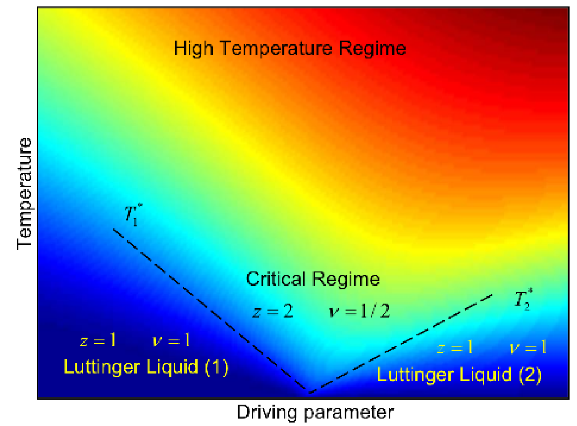
It is well known that 1D quantum systems exhibiting diverse phase transitions are a rich resource to study quantum criticality. In particular, the quasi-1D spin ladder models present rich quantum phase transitions induced by external magnetic fields [10]. Quantum criticality of 1D spin ladders is intimately related to the the SU(N) spin models with either integer or half odd integer spins. For even-leg spin ladders, the phase transition between the gapped and gapless phases is driven by the external magnetic field. The nature of the gapless phase illustrates the microscopic origin of criticality, see Fig. 1. When the spin gap is closed by an external field, the massive magnons of spin- states are restrained onto spin- states with a non-relativistic dispersion relation [7], . Here is the effective mass of magnons, is the energy gap and is the external magnetic field. Near the critical point, the magnons are not populated due to the strong magnetic field. Thus the magnons can be mapped onto the free-fermion universality class with dynamics exponent and and correlation length exponent . For the temperature below a crossover temperature , a single-component Luttinger liquid (LL) with linear dispersion is presented in the whole gapless regime, i.e. . Here and are the lower and upper critical fields, respectively. The physics of the gapless phase in one dimension is universally described by the Luttinger liquid with algebraic decay of the spin correlations at zero temperature, see experiments [11, 12, 13, 14, 15, 16]. For temperature , the correlation functions in LL phase decay exponentially. The LL parameters can be controlled directly by the external magnetic field. In a recent insightful experiment [17], this LL is shown to display a Fermi liquid nature at a renomalization fixed point. This marks an intrinsic connection between the two low energy theories: LL physics in 1D and Fermi liquid in higher dimensions. In contrast, spin triplet excitations in spin ladders in higher dimensions can be described as Bose-Einstein condensed (BEC) magnons [18].
In most of the integrable models, the eigenvalues can be obtained by means of the Bethe ansatz wave function. The Bethe ansatz wave function actually converts the Schrödinger equation of a many-body problem into a set of algebraic equations which are called the Bethe ansatz equations. These algebraic equations describe the roles of individual particles in the presence of many others. The summation of such complex individual roles often leads to a global coherent state, i.e. excitations can form a collective motion of spin and charge density waves with different velocities (behave like bosons) which are called the LL in spin and charge degrees of freedom.
These studies show that low temperature thermodynamics of the LL in the quantum disordered phase and collective thermal excitations in quantum critical regime have significantly different critical behaviour, see Fig. 2. The collective behaviour in the quantum critical regime is determined by the thermal excitations of the ground state. Modifying the Yang-Yang grand canonical thermodynamic approach [19], the equation of states of 1D many-body systems can be obtained in entire physical regimes. However, the Yang-Yang grand canonical description of the thermodynamics of integrable models is always much involved due to the complexity of microscopic roles. A new approach to treat thermodynamics of integrable systems [20, 8, 9] allows one to capture essential many-body physics in a rigorous way, including quantum criticality and quantum correlations.
The 1D spinless Lieb-Liniger gas [21, 22] and the spin-1/2 Fermi gas [23, 24, 25] are among the most extensively studied integrable many-body systems in quantum statistical mechanics. They exhibit novel quantum critical phenomena, and have had tremendous impact in quantum statistical mechanics. The quantum criticality of these models involves a universal crossover from the relativistic LLs with dynamic exponent and correlation exponent to free fermion quantum criticality with the dynamic exponent and correlation exponent , see Fig.2. In this figure, the dashed lines indicate crossover temperatures which separate the quantum critical regime with a nonrelativistic dispersion from a relativistic LL phases at low temperatures. In the critical region, both correlation length and thermal wave lengths are proportional to . Therefore, thermal and quantum fluctuations couple strongly at quantum criticality. In this scenario, recent breakthroughs in the experiments on trapped ultracold bosonic and fermionic atoms confined to one dimension has provided a better understanding of significant quantum statistical effects and quantum correlations in many-body systems, see review [22, 25]. In the present review, we briefly discuss quantum criticality and the universal nature of quantum liquids for these archetypical solvable models, i.e. Lieb-Liniger Bose gas, spin-1 Bose gas, the Gaudin-Yang model and large spin Fermi gases.
The paper is organised as follows. In Sec. II, we discuss quantum criticality and universal thermodynamics of the Lieb-Linger model. In Sec. III, quantum critical behaviour of the 1D spin-1 Bose gas with antiferromagnetic spin-spin interaction is discussed in terms of the grand canonical ensemble. In Sec. IV we discuss many-body critical phenomena and the Fermi liquid nature in the Yang-Gaudin model. Section V presents an outlook on quantum criticality of large spin Fermi gases and discusses new trends in exactly solvable systems.
II II. Quantum criticality of Bose gases
II.1 Lieb-Liniger model
The 1D Lieb-Liniger model [21] of interacting bosons is a prototypical Bethe ansatz integrable model, see the review [22, 26, 30]. The model is described by the Hamiltonian
| (1) |
in which spinless bosons, each of mass , are constrained by periodic boundary conditions on a line of length and is an effective one-dimensional coupling constant with scattering strength in a quasi-1D confinement. Here is the 1D scattering length with and the numerical constant [31]. The dimensionless interaction strength is defined by , where is the linear density.
Experimental studies of this model by using cold bosonic atoms over a wide range of tunable interaction strength between atoms have demonstrated the unique beauty of the Bethe ansatz integrability, see a feature review article [32]. These include the ferminization of the Tonks-Girardeau gas [33, 34, 35], quantum correlations [36, 37], thermolization [38], Yang-Yang thermodynamics [39, 40], the super Tonks-Girardeau gas [41], quantum phonon fluctuations [42, 43], elementary excitations [44], etc. There are more experimental developments with the Lieb-Liniger model, see review [22, 25].
Yang and Yang [19] introduced the particle-hole grand ensemble to describe the thermodynamics of the model in equilibrium, which is later called the thermodynamics Bethe ansatz (TBA) method by Takahashi [45]. At finite temperatures the equilibrium states become degenerate. Yang and Yang showed that true physical states can be determined by the minimisation conditions of Gibbs free energy subject to constraints on the roots of the Bethe ansatz equations, see a commentary in [46]. In terms of the dressed energy determined by the particle density and hole density with respect to the quasimomentum at finite temperature , the Yang-Yang equation is given by
| (2) |
where is the chemical potential, is the bare dispersion and kernel function . The dressed energy plays the role of excitation energy measured from the energy level , where is the Fermi-like momentum. The pressure are given in terms of the dressed energy by
| (3) |
Eq. (2) and (3) present a grand canonical description of Bethe ansatz equations for the integrable Lieb-Liniger Bose gas. It turns out that the Yang-Yang grand canonical description is an elegant way to analytically access thermodynamics, LL physics and quantum criticality [9, 47]. From the TBA equation (2), it is obvious that the pressure (3) reduces to several limiting cases, i.e. the classical Boltzmann gas with the de Broglie wavelength , free Fermi gas and free Bose gas
| (4) |
Where is the standard polylogarithm function. This result suggests that the TBA equation (2) encodes three statistics, Boltzmann statistics, Fermi-Dirac statistics and Bose-Einstein statistics in different limits.

Although it is generally believed that there does not exist a quantum phase transition at finite temperatures in this model, for grant canonical ensemble, there exists one critical point, i.e. chemical potential , which separates the vacuum from the filled “Fermi sea” of bosons at zero temperature. It is shown that the TBA equation (2) becomes dimensionless in term of a rescaled temperature , here we defined the interaction energy . At low temperatures, i.e. , the TBA equation (2) captures universal critical behaviour near . This can be clearly seen from the finite temperature phase digram of this model which was presented in see Fig.3. Here entropy in plane presents a universality class of quantum criticality associated quantum phase transition from vacuum into the LL phase. The right crossover temperature separates quantum critical regime with a nonrelativistic dispersion from the relativistic LL with exponent and correlation exponent . The regime and can be taken as a semiclassical gas, where the de Broglie wavelength is much smaller than the inter-particle mean spacing with the density . In this ideal gas phase, there is no ”Fermi surface”. The correlation behaves different from the algebraic behaviour in the LL phase [48].
Despite the equation (2) can be numerically solved for arbitrary strong interaction strength at all temperatures, understanding universal nature of such archetypical many-body model acquires additional analytical finite temperature thermodynamics. In [9], Guan and Batchelor calculated the thermodynamics of the model in analytic fashion using the polylog function. The pressure can be cast into the form
| (5) |
where
| (6) |
Here . This makes no need to numerically solve the integral equation (2) for critical phenomena at the temperatures below the degenerate temperature .
Further more, to the leading order, the free energy follows as the field theory form
| (7) |
where the central charge . For strong coupling regime, is the ground state energy per length and the sound velocity are given by
| (8) | |||||
| (9) |
This implies that for temperatures below a crossover value , the low-lying excitations have a linear relativistic dispersion relation, i.e. of the form . If the temperature exceeds this crossover value, the excitations involve free quasiparticles with nonrelativistic dispersion. This crossover temperature can be identified from the breakdown of linear temperature-dependent specific heat, i.e.
| (10) |
see the Fi. 4.

In the quantum critical regime, the density obeys the universal scaling form. It was proved [9] that the thermodynamic functions of this model such as the density and compressibility can be cast into the universal scaling forms [1, 3]
| (11) | |||||
| (12) |
with dimensionality . From the equation of state (5), the scaling function is
| (13) |
for which reads off the background density and the critical exponent with the correlation length exponent . The free fermion criticality revealed from (12) naturally comes from the fact that near the critical point the system has low density and strong interaction, i.e. Tonks-Girardeau regime. Meanwhile, the compressibility satisfies the scaling form (12) with and the background density .
In the realistic experiment, the quantum criticality (12) can be mapped out from the density profile of the trapped gas at finite temperature. Within the local density approximation, the chemical potentials in the equation of state (5) as well as in the TBA equation (3) are replaced by the local chemical potentials given by
| (14) |
Here the is the trapping center chemical potential which can be fixed by the total number in the trap. The external potential is defined as with harmonic frequency and the character length for the harmonic trap is . One can read off the dynamic exponent and the correlation length exponent from the density curves with a proper temperature scaling at different temperatures [50].
Moreover, the 1D integrable critical system, such as the LL, gives rise to the power law behaviour of long distance or long time asymptotics of correlation functions. Using the conformal field theory (CFT), which preserves angles, enables one to obtain asymptotic behaviour of correlation functions. For transformation and , the primary fields transform as
| (15) |
Where are two real numbers called the conformal weights of the field . The correlation functions of these primary fields were given as [51, 53]
| (16) |
If we set (), where is the Euclidean time and is the velocity of light. The two-point correlation function for primary fields with the conformal dimension becomes
| (17) |
The conformal dimensions can be read off from the finite-size corrections of low-lying excitations via Bethe ansatz solutions. Moreover, by replacing with in the conformal map , conformal invariance gives a universal form of correlation functions with exponential decay for a large distance asymptotic [53, 54]. The critical Hamiltonian can be approximately described by the conformal Hamiltonian which is described by the generators of underlying Virasoro algebra and the central charge . For , then the conformal dimensions characterizing the power law decay of the correlation functions at infinity depend continuously on the model parameters. In particular, the LL is specified by the central charge Virasoro algebra, for examaple, the Gaussian model [55, 56]. Close to criticality, the dispersion relations for 1D quantum systems are approximately linear. Conformal invariance predicts that the energy per unit length has a universal finite size scaling form where is the ground state energy per unit length for the infinite system and is a universal term related the conformal weights. Consequently, the calculation of the critical exponents of the critical models can reduce to calculation of low-lying excitation spectra. Thus the finite-size low-lying corrections to the ground state energy essentially determine the asymptotic behaviour of the correlation functions of the critical models, see [26, 57].

Although thermodynamics of the Lieb-Linger is accessible for whole temperature regime, the dynamic density-density correlation functions are difficult to calculate in analytical fashion [27]. Along this line, Caux and his coworkers have devoted systematic study on zero and finite temperature dynamical correlations [28, 29] based on the Bethe ansatz equations of the Lieb-Linger gas. The density-density correlation functions in Fourier space give the dynamical structure factor
| (18) |
with the density . At zero temperature, the dynamical structure factor can be represented as a sum of matrix elements of the density operator in the basis of Bethe eigenstate , i.e.
| (19) |
with . The static structure factor is given by . At finite temperature, density-density function becomes
| (20) |
where is the thermal equilibrium state. With the help of the Bethe ansatz solution and f-sum rule, the static dynamical factor at zero was plotted in terms of the interaction strength, see Fig. 5. The full dynamic correlations at finite temperatures have been studied recently in [29].
On the other hand, due to linear dispersion, the correlation functions of the system can be calculated within Bosonization approach [58, 22, 59]. The one-particle static density matrix is given by
Where the function and are dimensionless coefficients. is the linear density. In the thermodynamics limit, , . is the Luttinger parameter which determines the asymptotic behaviour of the correlation functions of the critical system. In thermodynamic limit, the leading order of one-particle correlation . One can observe that the oscillation terms become more important as the Luttinger parameter decreases. In strong coupling limit, the Luttinger parameter is given by [60]
| (21) |
The density-density correlation function is given by
In the Tonks-Girardeau limit, the density correlation function reads
| (22) |
It is particularly interesting that the condensate fraction of the Lieb-Liniger model displays finite-size critical scaling behaviour [61]. At , the Bose-Einstein condensation for the 1D Lieb-Linger gas with repulsive short-range interactions meets the Penrose and Onsager criterion by taking a particular large size limit. It is shown that if the interaction strength is given by a negative power of particle number , i.e. , the condensate fraction is nonzero and constant in various thermodynamic limits. Here is a density-independent amplitude and is an exponent. is the largest eigenvalue of the one-particle reduced density matrix, which can be numerically evaluated by the Bethe ansatz equations [61]. Thus the Lieb-Liniger gas does show Boson-Einstein condensation in the sense of Penrose and Onsager criterion.
Despite Lieb-Liniger is the simplest integrable model, it has rich many-body phenomena and gives deep insight into higher dimensional physics of many-body systems. The exact results for various observables of the Lieb-Liniger model at T=0 and at finite temperature were obtained by using field theory methods, i.e. the repulsive Lieb-Liniger Bose gas can be obtained as the nonrelativistic limit of the sinh-Gordon model [62, 63]. The local two- and three-body correlations have been calculated from the powerful field theory methods [64, 65]. In particular, Haller et al. [41] ] made an experimental breakthrough by observing a metastable highly excited gas-like phase Ð called the super Tonks-Girardeau gas Ð in the strongly attractive regime of bosonic Cesium atoms. The super Tonks-Girardeau gas was predicted theoretically by Astrakharchik et al. [66, 67] using Monte Carlo simulations and confirmed by Batchelor et al. [68] using the integrable interacting Bose gas with attractive interaction. The study of transition dynamics from Tonks-Girardeau gas [69] to attractive Tonks-Girardeau phase gives a further understanding of such metastable states in many-body systems [70]. This gas-like excitation state can be viewed as more strongly correlated Tonk-Girardeau gas with metastable criticality [71]. In that paper, the authors proved that the excited gas-like states in the super Tonks-Girardeau gas are more favourable in certain strongly attractive interaction regime in comparison with the excitations of the cluster states of different sizes.
In regard to the highly excited state, the splitting up of the Fermi sea of the 1D Lieb-Lininger gas displays interesting properties associated with multiple Fermi momenta [72]. In this regard, the Fermi sea splitting leads to consequences on the spectrum of such highly excited states with multiple Fermi seas. In particular, the dynamical structure factor displays threshold singularities at each edges of separated Fermi seas, see Fig. 6. The linearization of spectrum near each Fermi point also gives rise to the effective LL description of the Fermi sea splitting phenomena.

The Lieb-Liniger model provides a genuine setting to examine subtle many-body physics. The model presents the Tonks-Girardeau gas as the repulsion tends to infinity. In fact, the energy can be continuous in the limits . Such a novel connection at the results in a practicable quantum holonomy where the quantum states do not come back to the original ones after a cyclic changes of the interaction strength [73]. Beyond quantum holonomy, the complexification of the interaction and metastable quantum criticality of the supper Tonks-Girardeau gas [71] will further stimulate study of quantum liquid phase in excitations and non-Hermitian systems where the linear dispersion spectrum can be robust.
II.2 Spinor Bose gases
Large spin Bose gases have a rich phase diagram and exhibit various phases of quantum liquids [74] . The physics of spin-1, spin-2 and spin-3 bosons has been investigated in experiments with Na, 87Rb and 52Cr cold atoms. Spinor ultracold gases with large spins in one dimension present novel ferromagnetism and various spin liquids [22]. The spinor Bose gases with spin-independent short range interaction have a ferromagnetic ground state, [75, 76]. This nature was well invested in the two-component spinor Bose gas with spin-independent s-wave scattering [77, 78, 79] and the integrable multi-component Bose gases [83, 85]. At low energy level, the 1D two-component spinor Bose gas can be described by an effective Hamiltonian with spin-charge separation [80, 79], i.e. with charge density excitations and spin excitations
| (23) |
Where the sound velocity and is the Luttinger parameter in charge sector. and are the bosonic fields of density and phase satisfying the communication relation . The spin excitations can be described by the ferromagnetic Heisenberg chain with the effective coupling strength for strong coupling regime. Where is the pressure of the gas. In this strong coupling regime, i.e. , the specific heat exponent for the spinor Bose gas behaves as which is different from the Lieb-Liniger gas for which . In long wave length limit, the spin wave excitations over the ferromagnetic ground stat is given by [81, 82]. Here is the effective mass. For strong coupling, it is given by
| (24) |
We see that the effective mass takes the maximum value for . This means that by moving one boson with down spin, one has to move all the particles with up spins.
In contrast, the 1D spin-1 bosons with repulsive density-density and antiferromagnetic spin-exchange interactions [84, 86, 87, 88] exhibit either a spin-singlet paired ground state or a fully polarized ferromagnetic ground state. For the external field less than a lower critical field, the antiferromagnetic interaction leads to an effective attraction in the spin-singlet channel that gives rise to a quasi-condensate of singlet bosonic pairs. In this phase, the low energy physics can be characterized by a spin-charge separation theory of the LL describing the charge sector and a non-linear sigma model describing the spin sector [86]. It was shown that this model provides an integrable regularization of the nonlinear sigma model. On the other hand, the solely ferromagnetic quasi-condensate of fully polarized bosons occurs as the external field exceeds an upper critical field. Exact Bethe ansatz solution of this model provides deep insights into understanding competing ordering with quantum criticality [89, 90].
The Hamiltonian of the 1D spin-1 bosons with repulsive density-density and antiferromagnetic spin-exchange interactions reads [84]
| (25) |
that describes particles of mass confined in 1D to a length with -interacting type density-density and antiferromagnetic spin-exchange interactions between two atoms. In the above equations, is the spin-1 operator with -component . The interaction parameters and where the interaction strength is given by . Here represents the -wave scattering length in the total spin channels. stands for the Zeeman energy, where is the external field and the total spin in the -component. The model (25) has two conserved quantities, and the total particle number . In this model, the number of particles in a particular spin state is no longer conserved.

The model with antiferromagnetic spin-exchange interaction for is exactly solvable by the Bethe ansatz [84]. In grand canonical ensemble, thermodynamics of the model are determined by the the TBA equations (see [87] for details). In terms of the dressed energies , and for unpaired states, paired states and spin strings, the TBA equations read
| (26) | |||||
with . Here the symbol denotes the convolution , the functions are the same as the above and was given in [87].
The phase diagram of the model (25) presents a significant understanding of quantum phase transitions induced by any driving force, such as external fields, chemical potential, density and interaction strength. Exact solution of the model does provide precise determination of the phase diagram in an analytical way. The full phase diagram is presented in plane, see Fig. 7. The model exhibits three quantum phases at zero temperature: spin-singlet paired bosons , ferromagnetic spin-aligned bosons , and a mixed phase of the pairs and unpaired bosons . stands for the vacuum. The spin-singlet paired phase involves two types of pairs: pairs with different spin states and pairs of two bosons. The phase boundaries in the plane are essential for determining the quantum criticality of the model.
The model exhibits the ground state of either spin-singlet pairs or ferromagnetic fully-aligned bosons or co-existence of pairs and single bosons. The driving force like chemical potential and external field can drive the system from one ground state to another so that the associated quantum phase transition leads to universal critical phenomena. In canonical ensemble, the system presents a gapped phase for the external field less than a lower critical field . For the external field excesses a upper critical field , the fully- spin-aligned bosons form a ferromagnetic ground state. for an intermedium field, i.e. , the ground state gives the mixture of the pairs and single bosons of state . For strong coupling region the critical fields read
The quantum phase transitions driven by a magnetic field provide insight into large spin magnetism and universal criticality of the model. At low temperatures, the three zero temperature quantum phases, i.e., the phase of singlet pairs, ferromagnetic phase of spin-aligned atoms and the mixed phase of pairs and single atoms, could form the relativistic LL of bound pairs (), LL of single atoms () and a two-component LL () of paired and single atoms, respectively. This Luttinger liquid nature is evidenced from the universal form of the entropy
where the velocities can be calculated by the TBA equations (26) for full interaction strength. For strong coupling limit, one can obtain explicit forms of the velocities
Beyond crossover temperatures , the low energy LL physics breaks down, i.e. the dispersion of either bound pairs or unpaired single atoms becomes nonrelativistic. These critical fields and the crossover temperatures can be worked out in a straightforward way. These are obviously evidenced in the contour plot of the entropy in the plane, see Figure 8. The criticality of the spin-1 Bose gas are described by the free fermion criticality of two Tonks-Girardeau gases with masses and .

In the vicinity of the quantum critical points and , the system exhibits two different quantum critical regimes. The scaling functions of density and compressibility in the critical regime near the critical points and can be cast into the universal form (12) with the driving parameter of instead the chemical potential , see [89] Nevertheless, all thermodynamical properties like magnetization and susceptibility associated with the phase transitions driven by the magnetic field were rescaled to the universality class of quantum criticality of free fermions. It turns out that these universal thermodynamical properties can be used to map out the bulk phase diagram through the 1D trapped gas at finite temperatures [89]. By reformulating the equation of state within the local density approximation (LDA) with a replacement in which is the position and is the trapping frequency, the density profile and thermodynamical properties can be obtained for the trapped gas.
III IV. Probing Wilson ratio and Contact with criticality
III.1 Critical phenomena of the attractive Fermi gas
The 1D -function interacting spin-1/2 Fermi gas is a prototypical exactly solved model in literature. This model exhibits rich physics of interacting fermions in 1D: from few-body physics to many-body phenomena, including polarons, FFLO-like pairing, LL, quantum criticality, Fermi liquid signature, see a recent review [25]. Here we briefly discuss how exact solutions provide insights into the universal feature of Wilson ratio [131] and Tan’s contact [91].
In order to accommodate a general quantum liquid theory for the non-spin-charge separated mechanism, we briefly introduce a two-component attractive Fermi gas which was historically referred as Yang-Gaudin model [92, 93]. The quantum many-body Hamiltonian describes fermions of mass with external magnetic field
| (31) |
in which the Zeeman energy is given by . As being mentioned before, the effective 1D interaction strength can be tuned from the weakly interacting regime () to the strong coupling regime () via Feshbach resonances and confinement-induced resonances [31]. () is the contact repulsive (attractive) interaction. Usually, one defines the interaction strength as and dimensionless parameter for convenience. Here we denoted the total density , the magnetization , and the polarization , where is the linear density and is the length of the system.
The model was solved by Bethe ansatz [92, 93], where the Bethe ansatz wave numbers are the quasimomenta of fermions satisfying the Bethe ansatz equations
| (32) |
Here and , with spin-down fermions. The parameters are the rapidities for the internal spin degrees of freedom. The energies of the ground state and all excited states are given in terms of these quasimomenta, i.e. .

In the attractive interacting regime, at zero temperature, the quasimomenta of two atoms with different spin states form two-body bound states, i.e., , whereas the momenta of excess fermions are real in quasimomentum space. The distributions of these quaismomenta comprise the complexity of many-body physics. At the zero temperature and under an external magnetic field, the attractive Fermi gas have three different ground states: a fully-paired phase for the external field is less than the lower critical field , a fully-polarized ferromagnetic phase for the external field is greater than the upper crtical field , and the significant Fulde-Ferrel-Larkin-Ovchinnikov (FFLO) [95, 94] like pairing phase for a intermedium field . In the grand canonical ensemble, the phase diagram in the plane presents a universality class of criticality of the 1D interacting fermions, see Figure 9. Experimental measurement of phase diagram of two-component ultracold 6Li atoms trapped in an array of 1D tubes through the finite temperature density profiles confirms theoretical predictions [123]. The experimental developments on studying this one-dimensional interacting fermions [124, 125, 126] advance our understanding of many-body physics from integrability.
At zero temperature, the FFLO correlations [96, 97, 98, 99, 100, 101, 102, 103, 104, 105, 106, 107, 108, 109, 110, 111, 112] are the major concern from theory and experiment. From Bethe ansatz point of view, the low energy excitations correspond to changes in particle numbers (pairs or unpaired fermions) close to Fermi points. As a consequence, the system exhibits local scale invariance, i.e. conformal invariance. Thus various correlation functions can be analytically calculated using conformal field theory [114, 115, 116], for example the one particle Green’s function,
| (33) | |||
the charge density correlation function
| (34) | |||
and the pair correlation
| (35) | |||
In the above correlation functions, for strong coupling regime, the exponents can be given explicitly in [114, 115]. We observe that the leading order for the long distance asymptotics of the pair correlation function oscillates with wave number , where . The oscillation in pair correlation is caused by an imbalance in the densities of spin-up and spin-down fermions, i.e., , which gives rise to a mismatch in Fermi surfaces between both species of fermions. This spatial oscillation shares a similar signature as the Larkin-Ovchinikov (LO) pairing phase [94]. This can be regarded as the existence of a quasi-long range order. At finite temperatures, these correlations decay exponentially in 1D systems. The average distance between the pairs is the same order as between the unpaired fermions. The pairs lose dominating nature and the critical temperature is . Therefore the 1D analog of FFLO spacial oscillation nature in the pair correlation function is unable to probe through the trapped Fermi gas at finite temperatures. Nevertheless a quasi-1D systems that the fermions can tunneling from one tube to another would give rise to a finite critical temperature for the existence of the ordered phase at finite temperatures [117], see Fig. 10.

At finite temperatures, full thermodynamics of the model is determined by the TBA equations [45] that give rise to the universal quantum criticality. In the grand canonical ensemble, the grand partition function is written in terms of the Gibbs free energy with respect to the magnetic field , chemical potential and entropy . At finite temperatures, the density distribution functions of pairs, unpaired fermions and spin strings involve the densities of ‘particles’ and ‘holes’ , here for single excess fermions and bound pairs. The dressed energies, and characterize the excitation energites for paired and unpaired fermions. The equilibrium states are determined by the minimization condition of the Gibbs free energy that gives rise to the TBA equations
| (36) | |||||
The function is the ratio of the string densities. The same mathematical notations as used in previous spin-1 Bose gas. The function is given in [30]. The Gibbs free energy per unit length is given by where the effective pressures of the unpaired fermions and bound pairs are given by
with for unpaired fermions and for paired fermions. The TBA equations (36) indicate that the band energies of the bound pair and single particle depend on the changes of the pressures of bound pairs and excess fermions. The function originated from the two-body scattering amplitude encodes interaction effect. In these equations with proper expansion, one can obtain the similar first- and second-order Landau coefficients which reveal the forward scattering phase shift like the quasiparticle energies in Fermi liquid [118]. Later we shall briefly introduce such connection to the Wilson ratio in the attractive Fermi gas.
The phase diagram has been worked out by Orso [119] and by others [120, 121] using BA equations, which describe the ground state within a canonical ensemble. In terms of the dimensionless quantities , , and , where is the binding energy, the phase diagram is shown in Fig. 11. It consists of three phases: fully paired phase , ferromagnetic phase , and partially paired or (-like) phase. The system has spin population imbalance caused by a difference in the number of spin-up and spin-down atoms. These critical phase boundaries have been discussed in [8].

At low temperatures and strong coupling regime, the equation of states for the strongly attractive gas has been obtained by Guan and Ho in [8]. The analytical expression of the total pressure was presented for the regime and [8]. The dimensionless pressure of the system was found to be [8]
| (37) |
where
| (38) | |||||
| (39) |
Here
This term indicates that the spin degree of freedom ferromagnetically couples to the unpaired Fermi sea. In fact, this spin wave contribution to the function is negligible due to an exponentially small contributions at low temperatures. Although this equation of state (37) was derived in the regime for strong attraction and low temperatures, it presents a new theoretical scheme to treat quantum criticality of 1D ultracold Fermi gases with arbitrary interaction strength by employing analytical methods. The key observation is that the dimensionless form of the pressure of the system
| (40) |
can be expressed as a universal scaling form near quantum phase transitions
| (41) |
Where is the background pressure before quantum phase transition. In the second term is a dimensionless scaling function. The critical fields and present the phase boundaries in Fig. 11 [8]. In the above equations, are the dimensionless pressures of bound pairs and single fermions. The existence of the scaling form of Eq. (41) illustrates the microscopic origin of quantum criticality and provide analytic insight into continuum field theory that describes universal scaling theory in the vicinities of critical points. Thus the thermodynamical properties can be cast into universal scaling forms such as density and compressibility as presented in Eqs. (11) and (12). The density, compressibility, magnetization and susceptibility have the following scaling forms
| (42) | |||||
| (43) | |||||
| (44) | |||||
| (45) |
with the exponents and . The scaling functions and can be worked out explicitly from the TBA equations (36) in the region . From the equation of state (37), one can analytically examine quantum criticality of the model in an harmonic trap [122]. Here we demonstrate that the dimensionless susceptibility near the two critical points, i.e., in the vicinity of the critical points and , presents a universal scaling form
| (46) |
For strong attraction and near the lower critical point , there is no background susceptibility, i.e. . The constant with . In the above equations we used the dimensionless units and . The scaling form (46) reads off the universality class of quantum criticality of the dynamical critical exponent and correlation length exponent . We plot this scaling law of susceptibility near two critical points for fixed values of magnetic field in Fig. 12. In contrast, near the upper critical point , there is a background susceptibility. The universal form of susceptibility given in (46) with the following constants
maps out the quantum criticality with universal dynamical critical exponent and correlation length exponent for the phase transition from the FFLO to the normal free Fermi gas.

III.2 Wilson ratio in one dimension
In the scenario of universal low energy physics, Landau Fermi liquid theory [127, 128, 129] describes universal matter of quasiparticles in typical electronic metals, Kondo problem and He-3 liquid etc. The fermion excited outside the Fermi surface adiabatically evolves into a quaisparticle with the same charge, spin and momentum. These quasiparticles at the Fermi energy have an infinite lifetime. Even for these systems with strong interaction, such quasiparticle excitations still resemble the free fermions with a renomalized excitation energy . Here is the effective mass of quasiparticles and is the Femi momentum. Consequently, the effective magnetic moment and the mass of the quasiparticle are renomalized in terms of Landau parameters during the scattering process close to the surface. For forward scattering process, interaction just changes effective mass in the density of state. The specific heat increases linearly with the temperature as
| (47) |
because only the electrons within near the Fermi surface contribute to the specific heat. The susceptibility is independent of temperature since only the electrons within near the Fermi surface contribute to the magnetization. More explicitly,
| (48) |
In the above equations is the Landau parameter. We see that the specific heat and susceptibility only depend on the density of state and Landau parameters in forward scattering process. This universal nature is captured by a dimensionless constant, i.e. the Wilson ratio [130, 131], which is defined as the ratio of the magnetic susceptibility to specific heat divided by temperature ,
| (49) |
The effective mass was canceled out in this ratio. Thus the Wilson ratio is a constant at the renormalization fixed point of the interacting fermionic systems, despite it involves two thermodynamic properties. For example, most weakly correlated metals this ratio is a unity . It was proved that by Wilson [131] in the Kondo magnetic impurity problem in low temperatures.
In contrast, in 1D many-body systems the quasiparticle description breaks down due to the fact that all particles participate in the low energy physics. The main reason for this is that the elementary excitations in 1D are still eigenstates. Therefore one can not find a simple operator, acting on the ground state, to get an individual quasiparticle excitation, unlike that in higher dimensional Fermi liquid. The low-lying excitations in 1D actually form collective motion of bosons, i.e., the LL. In this regard, one can say “there will be no Fermi liquid in one dimension” [132]. However, the 1D system is critical in the gapless phase of LL, which is regarded as the critical phase at the renormalization fixed point. In such a low energy sector, elementary excitations close to the Fermi point in 1D systems essentially determine the critical behaviour and universal thermodynamics of the LL. Despite a breakdown of the quasiparticle description in 1D, the Fermi liquid nature can be retained in low energy sector [133, 118, 134]. Typical phenomenon of spin-charge separation in 1D interacting system is described by the effective Hamiltonian
| (50) |
where the effective Hamiltonians in spin and charge are given by
| (51) |
for . Here and obey the standard Bose commutation relations . The interaction term characterizes the backscattering process. The are the Luttinger parameters and are the sound velocities in charge and spin sectors, respectively. In term of spin-charge separation, the Wilson ratio at the fixed renormalization point reads
| (52) |
This naturally suggests that for noninteracting systems the ratio is unity and there does not exist spin-charge separation mechanism. However, for a strong repulsion, the spin transportation tends to zero so that the Wilson ratio tends to . This signature was numerically confirmed for the 1D Hubbard model by the Bethe ansatz solution [134]. It was recently pointed out [135] that the Wilson ratio quantifying interaction effects and spin fluctuations presents the universal nature of quantum liquids for both Fermi liquid and Luttinger liquid. Beyond the spin-charge separation scenario, the two important features of the Fermi liquid are retained for the renornalaization fixed point phase in 1D Fermi gases on a general ground, namely the specific heat is linearly proportional to temperature whereas the susceptibility is independent of temperature. Nevertheless, exact Bethe ansatz solutions would provide an alternative but a precise way to capture the nature of Fermi liquid. This study provides an intrinsic connection between the Fermi liquid and the LL.
In the context of cold atoms, the effective magnetic field depends on the chemical potential bias . The magnetization depends on the difference between the spin-up and -down fermion densities . In general, for the attractive interaction, the homogeneous system is described by two coupled Fermi gases of bound pairs and excess fermions in the charge sector and ferromagnetic spin-spin interaction ordering in the spin sector. At low temperatures, the ferromagnetic spin waves contributions to the low energy physics are marginal. In contrast to the spin-charge separation in repulsive Fermi gas, only the charge density fluctuations dominate the low energy physics for the attractive Fermi gas. In order to work out the susceptibility universality, we define two effective chemical potentials for bound pairs and excess fermions
| (53) |
Where the total chemical potential is given by and is the binding energy. For fixed total density, by definition, the susceptibility can be written in term of two charge susceptibilities
| (54) |
Where the charge susceptibilities of bound pairs and excess fermions were defined by . In the above equations, and are the densities of pairs and excess fermions. This relation is general and independent of integrability. This means that the two physical processes, i.e. the break of pairs and alignment of the spins, occur paralelly. The effective susceptibilities for the renormalization fixed point LL of bound pairs and the LL of excess fermions are expressed as
| (55) |
The density stiffness parameters are obtained from for a Galilean invariant system, with for excess fermions and for bound pairs. For the strongly interacting regime (), these density stiffness are given by [135]
Here and are the density of excess fermions and pairs, respectively.
For the TBA dressed energies have Fermi points at with for excess fermions and bound pairs, thus the Fermi velocities of unpaired fermions and bound pairs are defined as
| (59) |
with . Where are the density distribution functions for excess fermions and pairs. Thus the finite-size corrections to the ground state energy and finite temperature corrections to the free energy [121, 113]
| (60) |
indicates a universal critical scaling of conformal field theory with central change [54]. In the above equations is the ground state energy in thermodynamic limit. The exact expressions for the velocities can be found from the relation . These expressions (60) are universal in regard to the low energy sector and valid for arbitrary interaction regime. The low-lying excitations are decoupled into two massless excitations within Fermi seas of bound pairs and single excess fermions which are described by two Gaussian theories.
In the strong coupling limit, the velocities are given by
| (61) |
with . Here and . Consequently, the specific heat for the two-component LL is given by
| (62) |
This result is valid for arbitrary interaction strength. This linear -dependence of the specific heat is a characteristic of the two-component LL with linear dispersions in branches of pairs and single fermions. Deviation from this universal LL specific heat (62) indicates a breakdown of the linear temperature-dependent relation. This naturally defines the crossover temperature which charaterizes a universal crossover from a relativistic dispersion into a nonrelativistic dispersion [136, 113].
Moreover, from the LL free energy (60) one can check that the susceptibility is temperature independent in the phase of the two-component LL. The separation signature of the susceptibility (54) and specific heat (62) naturally suggests that the two branches of gapless excitations in the 1D FFLO-like phase form two collective LLs. Thus the low energy (long wavelength) physics of the strongly attractive Fermi gas is described by an effective Hamiltonian
| (63) | |||||
as long as the spin fluctuation is frozen out, see a discussion in [138]. Here the fields with are the density and current fluctuations for the pairs and unpaired fermions. In this case, the current-current interaction becomes irrelevant in the gapless phase. Thus the low energy physics of the FFLO-like phase is described by a renormalization fixed point of the two-component TTL class, where the interaction effect enters into the above collective velocities, or equally speaking that the effective masses of the two LLs are varied by the interaction.

The linear temperature-dependent nature of the specific heat and the temperature-independent susceptibility retain the important features of the Fermi liquid. The Wilson ratio of the attractive Fermi gas is given by
| (64) |
for the two-component LL phase in the attractive Fermi gas. This simple relation valid for a wide range of 1D spin-1/2 interacting fermionic systems. This result is universal in terms of the density stiffness and sound velocity for pairs b and excess single fermions u. Fig. 13 shows that at finite temperatures the contour plot of can map out not only the two-component LL phase but also the quantum criticality of the attractive Fermi gas. It is worth noting that Wilson ratio for the 1D attractive Fermi gas is significantly different from the ratio obtained for the field-induced gapless phase in the quasi-1D gapped spin ladder [17], where the gapless phase is a single-component LL [137, 118]. Again, deviation from the Wilson ratio (64) gives the crossover temperature separating the LL from the free fermion liquid near the critical points. In contrast to the phenomenological LL parameter, the Wilson ratio provides a testable parameter for quantifying universal nature of quantum liquids of interacting fermions in one, two and three dimensions.

III.3 Critical behaviour of Contact in one dimension
Universal relations which hold independently of the interaction strength always attract great deal of attention from theory and experiment. The universal quantity called contact which has been for the first time found in unitary Fermi gases by Tan [91] provides new insight into two-body correlations in short distance limit, i.e. with , where is the density operator at position and is the contact and. Tan’s contact, which measures the two-body correlation at short distances in dilute systems, also remarkably presents the universality of many-body systems of ultra cold atoms [149]. It connects various properties of the system, ranging from the tail of large momentum distribution as , thermodynamics , high frequency dynamic structure factor and adiabatic relation with the changes in the scattering length , see [139, 140, 141, 142, 143, 144]. Here is the scattering length. The significant feature of Contact is that it can be applied to any many-body system of interacting bosons and fermions in 1D, 2D and 3D and exists in normal phase and superfluid phase. Tan’s contact leads to immediate implications in cold atomic physics [145, 146, 147].
The study of Tan’s relation in 1D many-body systems provides essential information on local pair correlations [148]. Recent study on the universality of Contact for the spin-1/2 Fermi gas shows that Contact remarkably connects quantum criticality of many-body systems [149]. Tan’s adiabatic contact in 1D is defined [148]. In practice, it reads
| (65) |
It connects various thermodynamical properties of 1D many-body systems via the general thermodynamical relations
| (66) |
In the above equations is the energy eigenvalue, is the entropy and is the magnetization. This relation provides insightful connections of Contact to thermodynamical properties via
| (67) |
With the help of Eq. (37) we can prove the novel existence of universal scaling behaviour of the Contact. In grand canonical ensemble, the contact is given by
| (68) |
Here is the total local pair correlation and is the pressure per unit length.
From the scaling form of the pressure (41), we see that critical fields and essentially depend on the interaction. So that the contact defined by (68) must possess scaling behaviour like other thermodynamical properties such as density, compressibility, magnetization and susceptibility. It was found [149] that the universal scaling forms of the contact and its derivative with respect to the driven parameter (or ) read
| (69) | |||||
| (70) |
where () is the background contact (derivative of the contact) which is temperature independent. The constant depend on the critical values of and . In the above equations and are the dimensionless scaling functions. The critical phenomena of Contact (70) are valid for full interaction strength. The finite temperature Contact shows that the scaling form (69) with the dimension for the model read off the dynamic exponent and the correlation exponent [149]. Fig. 14 shows the universal scaling behaviour for the phase transitions from vacuum to the fully paired phase and from fully-polarized phase to the partially-polarized phase through the numerical solution of the TBA equations (36). The scaling behaviour of the derivative of Contact with respect to the driving parameter was demonstrated in connections to various physical properties, see [149]. This finding sheds light on the universal feature of Tan’s contact in connection to quantum criticality in low and higher dimensions. In particular, it provides insights into the study of critical behaviour of the Contact near the critical temperature for the unitary Fermi gas [146].
IV V. Outlook
| No. | |||||||
|---|---|---|---|---|---|---|---|
| (i) | |||||||
| (ii) | |||||||
| (iii) |
Quantum criticality provide a promising way to explore a broad range of novel phenomena and hidden symmetries of quantum many-body systems, for example, the 1D quantum Ising model with both a transverse field and a longitudinal field displays the largest exceptional group E8 symmetry [150, 151]. A pedagogical review of theoretical results for the Ising model universality class, including S-matrix, correlation functions, integrability breaking, etc, was discussed in terms of integrable field theory and critical phenomena [179]. This hidden E8 symmetry was dramatically demonstrated in experiment [152, 153]. In this scenario experiments on quantum criticality of ultracold atoms [154, 155, 156, 157] open up a new way to explore critical phenomena in quantum many-body systems. Here it is appropriate to quote the insightful perspective on quantum criticality remarked by Coleman and Schoefield [2]: “Quantum criticality may be a highly effective catalyst for the formation of new stable types of material behaviour, providing an important new route for the design and discovery of new classes of material Ó.
Moreover, integrability with cold atoms offers a precise method to treat quantum critical phenomena in many-body systems of bosons and fermions, see review [25]. Along this line, it is highly desirable to study quantum criticality of large spin systems with high symmetries in this exact manner. The large spin systems of cold atoms exhibit rich internal structures that may result in new quantum phases and multi-component LLs [158, 159, 160, 161, 162, 163]. In this regard, the spin-3/2 fermionic systems are likely to provide an ideal model towards a precise understanding of large spin non- symmetries.
The simplest high spin Hamiltonian [164, 165, 166, 167]
| (71) |
describes dilute spin-3/2 atomic gases of fermions with contact interaction constrained by periodic boundary conditions to a line of length . Here the summation is carried out for and . In the above equations projection operator projects the total spin- state onto spin- in the -direction of two colliding atoms and . The interaction strength in the channel is given by . It is remarkable that the model exhibits different spin symmetries , and while the integrability is preserved [168], see the Table I. This model has rich spin pairing states, i.e. spin- pairs with which lead to the Fulde-Ferrel-Larkin-Ovchinnikov like pair correlations and multi-component LLs for all interaction strength. These spin- pairs form two subspaces, with interaction strength and respectively

It is very interesting that the model exhibits FFLO-like pair correlation function in a mixed phase of pairs and single fermions of atoms
| (78) |
where , and are the densities of unpaired atoms and atomic pairs , respectively. The quantum criticality of the model for the phase transition from the vacuum into the FFLO phase is governed by the scaling functions
where is the Fermi-Dirac function and . Indeed the scaling functions of density and compressibility (IV) identify the dynamic critical exponent and correlation length exponent , see the Fig. 15. This preliminary study of quantum criticality of large spin fermionic systems opens a way to treat high spin phenomena in an analytical fashion. It is particularly interesting to probe Wilson ratio and Tan’s contact with quantum criticality of large spin systems.
Moreover, recent experimental developments with ultracold atoms provide exciting opportunities to test quantum dynamics of many-body systems. In particular, the quantum dynamics of mobile spin impurity give deep understanding of the motion of impurity and polaronic behaviour [169]. Microscopic observation of two magnon bound states helps one to understand quantum walks of magnons predicted by the Bethe ansatz solvable model [170, 171]. This research suggests further investigation of quantum quench dynamics of 1D interacting bosons and fermions. Essentially, in the 1D Lieb-Liniger gas of bosons, two types of excitations–Bogoliubov phonons and type II excitations, give rise to significantly different dynamics. The type II excitation is regarded as the quantum dark soliton [172]. Creating such type II excitations in the trapped gas would demonstrate unique 1D quantum dynamics through a 2D array of 1D tubes. Quantum quench dynamics of interacting fermions and bosons in 1D play an essential role in understanding nonequilibrium evolution of isolated systems beyond the usual thermal Gibbs mechanism [173]. The generalized Gibbs ensemble [174, 175, 176, 177, 178] is used in discussions of non-thermal distributions in isolated systems with conserved laws. Recently there have been several papers focusing on the study of quench dynamics in regard to the validity of the generalized Gibbs Ensemble (GGE), see [180, 181, 182, 183, 184], etc. This research has been becoming a new frontier in cold atoms and condensed matter physics. However, understanding thermalization of isolated many-body systems still imposes a big theoretical challenge.
Acknowledgment. The author thanks Tony Guttmann, Murray T Batchelor, Helen Perk, Angela Foerster, Jean-Sebastien Caux, Tetsuo Deguchi and zoran ristivojevic for discussions and help with proofreading. This work has been supported by the National Basic Research Program of China under Grant No. 2012CB922101 and NNSFC under grant numbers 11374331. He has been partially supported by the Australian Research Council. He acknowledges the Beijing Computational Science Research Center and KITPC, Beijing for their kind hospitality.
References
- [1] S. Sachdev, Quantum Phase transitions (Cambridge University Press, 1999).
- [2] P. Coleman and J. Schofield, Nature 433, 226 (2005).
- [3] M. P. A. Fisher, P. B. Weichman, G. Grinstein and D. F. Fisher, Phys. Rev. B 40, 546 (1989).
- [4] M. Vojta, Rep. Prog. Phys. 66 (2003) 2069.
- [5] K. G. Wilson, Phys. Rev. B 4, 3174 (1971); Phys. Rev. B 4, 3184 (1971).
- [6] T. Senthil, Phys. Rev. B 70, 144407 (2004).
- [7] Y. Maeda, C. Hotta and M. Oshikawa, Phys. Rev. Lett. 99, 057205 (2007).
- [8] X.-W. Guan and T.-L. Ho, Phys. Rev. A 84, 023616 (2011).
- [9] X.-W. Guan and M. T. Batchelor, J. Phys. A 44, 102001 (2011).
- [10] E. Dagotto and T. M. Rice, Science 271, 618 (1996).
- [11] M Klanjsek et al., Phys. Rev. Lett. 101, 137207 (2008).
- [12] Ch. Ruegg et al., Phys. Rev. Lett. 101, 247202 (2008).
- [13] B. Thielemann et al., Phys. Rev. B 79, 020408R (2009).
- [14] V. O. Garlea et al., Phys. Rev. Lett. 100, 037206 (2008).
- [15] A. Zheludev et al., Phys. Rev. Lett. 100, 157204 (2008).
- [16] B. C. Watson et al., Phys. Rev. Lett. 86, 5168 (2001).
- [17] K. Ninios et al., Phys. Rev. Lett. 108, 097201 (2012).
- [18] T. Giamarchi et al, Nature Phys. 4, 198 (2008).
- [19] C. N. Yang and C. P. Yang, J. Math. Phys. 10, 1115 (1969).
- [20] E. Zhao, X.-W. Guan, W. V. Liu, M. T. Batchelor and M. Oshikawa, Phys. Rev. Lett. 103, 140404 (2009).
- [21] E. H. Lieb and W. Liniger, Phys. Rev. 130, 1605 (1963).
- [22] M. A. Cazalilla, R. Citro, T. Giamarchi, E. Orignac and M. Rigol, Rev. Mod. Phys. 83, 1405 (2011).
- [23] C. N. Yang, Phys. Rev. Lett. 19, 1312 (1967).
- [24] M. Gaudin, Phys. Lett. A 24, 55 (1967).
- [25] X.-W. Guan, M. T. Batchelor and C. Lee, Rev. Mod. Phys. 85, 1633 (2013).
- [26] V. E. Korepin, A. G. Izergin and N. M. Bogoliubov, Quantum Inverse Scattering Method and Correlation Functions, Cambridge University Press (1993).
- [27] P. Calabrese and J.-S Caux, J. Stat. Mech. (2007) P08032.
- [28] J.-S Caux and P. Calabrese, Phys. Rev. A 74, 031605(R) (2006).
- [29] M. Panfil and J.-S Caux, Phys. Rev. A 89, 033605 (2014).
- [30] M. Takahashi, Thermodynamics of One-Dimensional Solvable Models, Cambridge University Press (1999).
- [31] M. Olshanii, Phys. Rev. Lett. 81, 938 (1998); V. Dunjko, V. Lorent and M. Olshanii, Phys. Rev. Lett. 86, 5413 (2001).
- [32] M. T. Batchelor, Int. J. Mod. Phys. B 28, 1430010 (2014).
- [33] P Paredes, et al. Nature (London) 429, 277 (2004).
- [34] T. Kinoshita, T. Wenger and D.S. Weiss, Science 305, 1125 (2004).
- [35] T. Kitagawa et al., Phys. Rev. Lett. 104, 255302 (2010).
- [36] T. Kinoshita, T. Wenger and D.S. Weiss, Phys. Rev. Lett. 95, 190406 (2005).
- [37] V. Guarrera, et al. Phys. Rev. A 86, 021601(R) (2012).
- [38] T. Kinoshita et al., Nature 440, 900 (2006).
- [39] A. H. van Amerongen et al.., Phys. Rev. Lett. 100, 090402 (2008).
- [40] A. Vogler et al. Phys. Rev. A 88, 031603(R) (2013).
- [41] E. Haller et al., Science 325, 1224 (2009).
- [42] J. Armijo, T. Jacqmin, K. V. Kheruntsyan and I. Bouchoule, Phys. Rev. Lett. 105, 230402 (2010).
- [43] J. Armijo, Phys. Rev. Lett. 108, 225306 (2012).
- [44] N. Fabbri, et al. arXiv:1406.2176.
- [45]
M. Takahashi, Prog. Theor. Phys. 46, 401 (1971);
M. Takahashi, Prog. Theor. Phys. 46, 1388 (1971);
M. Takahashi, Prog. Theor. Phys. 47, 69 (1972);
M. Takahashi, Prog. Theor. Phys. 50, 1519 (1973);
M. Takahashi, Prog. Theor. Phys. 52, 103 (1974). - [46] C. N. Yang, Selected papers 1945-1980, W. H. Freeman and Company (1983).
- [47] M. Wang et al., Phys. Rev. A 87, 043634 (2013).
- [48] F. Göhmann and V. E. Korepin, Phys. lett. A 260, 516 (1999).
- [49] Numerical solution of the TBA equation (2) was prepared by Dr. Xiangguo Yin from Center for optical quantum technologies, Hamburg University.
- [50] M.-S. Wang et al. Phys. Rev. A 87, 043634 (2013).
- [51] A. A. Belavin, A. M. Polyakov, and A. B. Zamolodchikov, Nucl. Phys. B 241, 333 (1984).
- [52] J. Voit, Rep. Prog. Phys. 58, 977 (1995).
- [53]
H. W. J. Blöte, J. L. Cardy, and M. P. Nightingale, Phys. Rev. Lett.
56, 742 (1986);
J. L. Cardy, Nucl. Phys. B 270, 186 (1986). - [54] I. Affleck, Phys. Rev. Lett. 56, 746 (1986).
- [55] F. D. M. Haldane, Phys. Lett. A 81, 153 (1981).
- [56] F. D. M. Haldane, J. Phys. C 14, 2589 (1981).
- [57] F.H.L. Essler, et.al. The One-Dimensional Hubbard Model (Cambridge University Press, Cambridge, 2005).
- [58] T. Giamarchi, Quantum Physics in one dimension, Oxford University Press, Oxford (2004).
- [59] M Cazalilla, J Phys. B, 37, S1 (2004).
- [60] Z. Ristivojevic, arXiv:1403.3415.
- [61] J. Sato, E. Kaminishi, and T. Deguchi, arXiv:1303.2775.
- [62] M. Kormos, G. Mussardo, and A. Trombettoni, Phys. Rev. A 81, 043606 (2010).
- [63] M. Kormos, G. Mussardo, and B. Pozsgay, JSAT/2010/P05014.
- [64] M. Kormos, G. Mussardo, and A. Trombettoni, Phys. Rev. Lett. 103, 210404 (2009).
- [65] M. Kormos, G. Mussardo, and A. Trombettoni, Phys. Rev. A 83, 013617 (2011).
- [66] G. E. Astrakharchik et al., Phys. Rev. Lett. 95, 190407 (2005).
- [67] G. E. Astrakharchik et al., Phys. Rev. Lett. 92, 030402 (2004).
- [68] M. T. Batchelor et al., J. Stat. Mech. L10001 (2005).
- [69] M. D. Girardeau, J. Math. Phys. 1, 516 (1960).
- [70] S. Chen, L. Guan, X. Yin, Y. Hao and X.-W. Guan, Phys. Rev. A 81, 031609(R) (2010).
- [71] M. Panfil, J. D. Nardis and J.-S. Caux, Phys, Rev. Lett. 110, 125302 (2013).
- [72] T. Fokkema, I. S. Eliëns and J.-S. Caux, Phys. Rev. A 89, 033637 (2014).
- [73] N. Yonezawa, A. Tanaka, and T. Cheon, Phys. Rev. A 87, 062113 (2013).
- [74] T.-L. Ho, Phys. Rev. Lett. 81, 742 (1998); T.-L. Ho and S. K. Yip, Phys. Rev. Lett. 84, 4031 (2000).
- [75] E. Eisenberg and E. H. Lieb, Phys. Rev. Lett. 89, 220403 (2002).
- [76] K. Yang and Y.-Q. Li, Int. J. Mod. Phys. B 17, 1027 (2003).
- [77] B. Sutherland, Phys. Rev. Lett. 20, 98 (1968).
- [78] Y.-Q. Li, S.-J. Gu, Z.-J. Ying and U. Eckern, Europhys. Lett. 61, 368 (2003).
- [79] X.-W. Guan, M. T. Batchelor and M. Takahashi, Phys. Rev. A 76, 043617 (2007).
- [80] K. A. Matveev and A. Furusaki, Phys. Rev. Lett. 101, 170403 (2008).
- [81] J. N. Fuchs, D. M. Gangardt, T. Keilmann and G. V. Shlyapnikov, Phys. Rev. Lett. 95, 150402 (2005).
- [82] M. T. Bachelor, M. Bortz, X.-W. Guan and N. Oelkers, J. Stat. Mech.: Theory and Experiment, JSTAT/2006/P03016.
- [83] C. N. Yang and Y.-Z. You, Chinese Phys. Lett. 28, 020503 (2011).
- [84] J. Cao, Y. Jiang and Y. Wang, Europhys. Lett. 79, 30005 (2007).
- [85] Y. Jiang, J. Cao and Y. Wang, J. Phys. A 44, 345001 (2011).
- [86] F. H. L. Essler, G. V. Shlyapnikov and A. M. Tsvelik, J. Stat. Mech. (2009) P02027.
- [87] J. Y. Lee, X.-W. Guan, M. T. Batchelor and C. Lee, Phys. Rev. A 80, 063625 (2009).
- [88] G. V. Shlyapnikov and A. M. Tsvelik, New J. Phys. 13, 065012 (2011).
- [89]
C. C. N. Kuhn, X. W. Guan, A. Foerster, and M. T. Batchelor, Phys. Rev. A 85, 043606 (2012);
C. C. N. Kuhn, X. W. Guan, A. Foerster, and M. T. Batchelor, Phys. Rev. A 86, 011605(R) (2012). - [90] H.-M. Wang and Y.-B. Zhang, Physical Review A, 88, 023626 (2013).
- [91] S. Tan, Ann. Phys., 323, 2952 (2008); 323, 2971 (2008); 323, 2987 (2008).
- [92] C. N. Yang, Phys. Rev. Lett. 19, 1312 (1967).
- [93] M. Gaudin, Phys. Lett. A 24, 55 (1967).
- [94] A. I. Larkin, and Yu. N., Ovchinnikov, Sov. Phys. JETP 20, 762 (1965).
- [95] P. Fulde, and R. A. Ferrell, Phys. Rev. 135, A550 (1964).
- [96] A. E. Feiguin and F., Heidrich-Meisner, Phys. Rev. B 76, 220508(R) (2007).
- [97] M. Tezuka and M. Ueda, Phys. Rev. Lett. 100, 110403 (2008).
- [98] M. M. Rizzi, Polini, M. A. Cazalilla, M. P. Tosi, and R. Fazio, Phys. Rev. B 77, 245105 (2008).
- [99] A. R. Lüscher, M Noack, and A. M. Läuchli, Phys. Rev. A 78, 013637 (2008).
- [100] G. G. Batrouni, M. H. Huntley, V. G. Rousseau, and R. T. Scalettar, Phys. Rev. Lett. 100, 116405 (2008).
- [101] S. K. Baur, J. Shumway, and E. J. Mueller, Phys. Rev. A 81, 033628 (2010).
- [102] M. M. Parish, M. M., S. K. Baur, E. J. Mueller, and D. A. House, Phys. Rev. Lett. 99, 250403 (2007).
- [103]
X.-J. Liu, H. Hu, and P. D. Drummond, Phys. Rev. A
76, 043605 (2007);
X.-J. Liu, H. Hu, and P. D. Drummond, Phys. Rev. A 78, 023601 (2008). - [104] E. Zhao, and W. V. Liu, Phys. Rev. A 78, 063605 (2008).
- [105] J. M. Edge, and N. R. Cooper, Phys. Rev. Lett. 103, 065301 (2009).
- [106] T. Datta, Eur. Phys. J. B 67, 197 (2009).
- [107] J. C. Pei, J. Dukelsky, and W. Nazarewicz, Phys. Rev. A 82, 021603 (2010).
- [108] J. P. A. Devreese, S. N. Klimin, and J. Tempere, Phys. Rev. A 83, 013606 (2011).
- [109] J. Kajala, J., F. Massel, and P. Tö rmä, Phys. Rev. A 84, 041601(R) (2011).
- [110] A.-H. Chen, and X. Gao, Phys. Rev. B 85, 134203 (2012).
- [111] C. J. Bolech et al., Phys. Rev. Lett. 109, 110602 (2012).
- [112] H. Lu, L. C. Baksmaty, C. J. Bolech and H. Pu, Phys. Rev. Lett. 108, 225302 (2012).
- [113] E. Zhao, X.-W. Guan, W. V. Liu, M. T. Batchelor and M. Oshikawa, Phys. Rev. Lett. 103, 140404 (2009).
- [114] J.-Y. Lee and X.-W. Guan, Nucl. Phys. B 853, 125 (2011).
- [115] P. Schlottmann and A. A. Zvyagin, Phys. Rev. B 85, 205129 (2012).
- [116] J.-Y. Lee, X.-W. Guan, K. Sakai and M. T. Batchelor, Phys. Rev. B 85, 085414 (2012).
- [117] N. M. Bogoliubov and V. E. Korepin, Int. J. Mod. Phys. B 3, 427 (1989).
- [118] Y.-P. Wang, Int. J. Mod. Phys. B 12, 3465 (1998).
- [119] G. Orso, Phys. Rev. Lett. 98, 070402 (2007).
- [120] H. Hu, X.-J. Liu and P. D. Drummond, Phys. Rev. Lett. 98, 070403 (2007).
- [121] X.-W. Guan, M. T. Batchelor, C. Lee and M. Bortz, Phys. Rev. B 76, 085120 (2007).
- [122] X.-G. Yin, X.-W. Guan, S. Chen, and M. T. Batchelor, Phys. Rev. A 84, 011602(R) (2011).
- [123] Y.-A. Liao, A. S. C. Rittner, T. Paprotta, W. Li, G. B. Partridge, R. G. Hulet, S. K. Baur, and E. J. Mueller, Nature 467, 567 (2010).
- [124] H. Moritz, T. Stöferle, K. Günter, M. Köhl, and T. Esslinger, Confinement Induced Molecules in a 1D Fermi Gas, Phys. Rev. Lett. 94, 210401 (2005).
- [125] G. Zürn, F. Serwane, T. Lompe, A. N. Wenz, M. G. Ries, J. E. Bohn, and S. Jochim, Fermionization of Two Distinguishable Fermions, Phys. Rev. Lett. 108, 075303 (2012).
- [126] A. N. Wenz, G. Zürn, S. Murmann, I. Brouzos, T. Lompe, S. Jochim, From Few to Many: Observing the Formation of a Fermi Sea One Atom at a Time Science 342, 457 (2013).
- [127] L. D. Landau, Sov. Phys. JETP 3, 920 (1956).
- [128] L. D. Landau, Sov. Phys. JETP 5, 101 (1957).
- [129] L. D. Landau, Sov. Phys. JETP 8, 70 (1958).
- [130] A. Sommerfeld, Z. Phys. 47, 1 (1928).
- [131] K. G. Wilson, Rev. Mod. Phys. 47, 773 (1975).
- [132] A. Georges and T. Giamarchi, arXiv:1308.2684.
- [133] H. J. Schulz, G. Cuniberti and P. Pieri, arXiv:cond-mat/9807366.
- [134] D. C. Johnston et al., Phys. Rev. B 61, 9558 (2000).
- [135] X.-W. Guan, X. G. Yin, A. Foerster, M. T. Batchelor, C. H. Lee, H. Q. Lin, Phys. Rev. Lett. 111, 130401 (2013).
- [136] Y. Maeda, C. Hotta and M. Oshikawa, Phys. Rev. Lett. 99, 057205 (2007).
- [137] H. J. Schulz, Int. J. Mod. Phys. B 5, 57 (1991).
- [138] T. Vekua, S. T. Matveenko and G. V. Shlyapnikov, JETP Lett. 90, 289 (2009).
- [139] E. Braaten, BCS-BEC Crossover and the Unitary Fermi Gas, Lecture Notes in Physics (Springer, 2011).
- [140] H. Hu, X.-J. Liu and P.D. Drummond, New J. Phys. 13, 035007 (2011).
- [141] E. V. H. Doggen, and J. J. Kinnunen, Phys. Rev. Lett. 111, 025302 (2013).
- [142] D. H. Smith, E. Braaten, D. Kang and L. Platter, Phys. Rev. Lett. 112, 110402 (2014).
- [143] Y. Yan and D. Blume, Phys. Rev. A 88, 023616 (2013).
- [144] G. B. Partridge, K. E. Strecker, R. I. Kamar, M. W. Jack and R. G. Hulet, Phys. Rev. Lett. 95, 020404 (2005).
- [145] J. T. Stewart, J. P. Gaebler, T. E. Drake and D. S. Jin, Phys. Rv. Lett. 104, 235301 (2010).
- [146] Y. Sagi, T. E. Drake, R. Paudel and D. S. Jin, Phys. Rev. Lett. 109, 220402 (2012).
- [147] S. Hoinka, M. Lingham, K. Fenech, H. Hu, C. J. Vale, J. E. Drut and S. Gandolfi, Phys. Rev. Lett. 110, 055305 (2013).
- [148] M. Barth and W. Zwerger, Ann. Phys. 326, 2544 (2011).
- [149] Y.-Y. Chen, Y.-Z. Jiang, X.-W. Guan, and Q. Zhou, arXiv:1405.2256.
- [150] A. B. Zamolodichikov, Int. J. Mod. Phys. A 04, 4235 (1989).
- [151] M. Henkel, and H. Saleur, J. Phys. A 22, L513 (1989).
- [152] R. Coldea et al. Science 327, 177 (2010).
- [153] C. M. Morris et al. Phys. Rev. Lett. 112, 137403 (2014).
- [154] N. Gemelke, X. Zhang, C.-L Hung, and C. Chin, Nature 460, 995 (2009).
- [155] C.-L. Huang, X. Zhang, N. Gemelke, and C. Chin, Phys. Rev. Lett. 104, 160403 (2010).
- [156] C.-L. Huang, X. Zhang, N. Gemelke, and C. Chin, Nature 470, 236 (2011).
- [157] X. Zhang, C.-L. Hung, S.-K. Tung, and C. Chin, Science 335, 1070 (2012).
- [158] T.-L. Ho and S. Yip, Phys. Rev. Lett. 82, 247 (1999).
- [159] S.-K. Yip and T.-L. Ho, Phys. Rev. A 59, 4653 (1999).
- [160] C. Wu, Phys. Rev. Lett. 91, 186402 (2003).
- [161] C. Honerkamp and W. Hofstetter, Phys. Rev. Lett. 92, 170403 (2004).
- [162] A. V. Gorshkov et al., Nature Phys. 6, 289 (2010).
- [163]
M. A. Cazalilla, A. F. Ho and M. Ueda, New J. Phys. 11, 103033 (2009);
M. A. Cazalilla and A. M. Rey, arXiv:1403.2792. - [164]
C. Wu, Phys. Rev. Lett. 95, 266404 (2005);
Mod. Phys. Lett. B 20, 1707 (2006). - [165] P. Lecheminant, E. Boulat and P. Azaria, Phys. Rev. Lett. 95, 240402 (2005).
- [166] D. Controzzi and A. M. Tsvelik, Phys. Rev. Lett. 96, 097205 (2006).
- [167]
Y. Jiang, J. Cao and Y. Wang, Europhys. Lett. 87, 10006 (2009);
J. Phys. A 44, 345001 (2011). - [168] Y. Jiang, X.-W. Guan, J. Cao and H.-Q. Lin, preprint 2014.
- [169] T. Fukuhara et al. Nature Physics 9, 235 (2013).
- [170] T. Fukuhara et al. Nature 502, 76 (2013).
- [171] Liu and Andrei, arXiv:1311.1118.
- [172] J. Sato, R. Kanamoto, E. Kaminishi and T. Deguchi, Phys. Rev. Lett. 108, 110401 (2012).
- [173] M. Rigol, V. Dunjko, V. Yurovsky and M. Olshanii, Phys. Rev. Lett. 98, 050405 (2007).
- [174] M. Rigol, V. Dunjko and M. Olshanii, Nature 452, 854 (2008).
- [175] J.-S. Caux and F. H. L. Essler, Phys. Rev. Lett. 110, 257203 (2013).
- [176] J. Nardis, B. Wouters, M. Brockmann, and J.-S. Caux, Phys. Rev. A. 89, 033601 (2014).
- [177] G. Goldstein and N. Andrei, arXiv:1405.6365.
- [178] G. Goldstein, N. Andrei, arXiv:1309.3471.
- [179] G. Delfino, J. Phys. A 37, R45 (2004).
- [180] B. Pozsgay, arXiv:1406.4613.
- [181] B. Wouters, et al. arXiv:1405.0172.
- [182] M. Brockmann, et al. arXiv:1408.5075.
- [183] B. Pozsgay, at al. arXiv:1405.2843.
- [184] G. Goldstein, N. Andrei, arXiv:1405.4224