Kepler and the Long Period Variables

Erich Hartig¹¹ 1 Joint lead author Affiliation: University of Vienna, Department of Astrophysics, Türkenschanzstrasse 17, A-1180 Vienna, Austria Email: erich.hartig@univie.ac.at Jennifer Cash¹ Affiliation: Department of Biological and Physical Sciences, South Carolina State University, P.O. Box 7024, Orangeburg, SC 29117,USA Email: jcash@physics.scsu.edu Kenneth H. Hinkle Affiliation: National Optical Astronomy Observatories
P.O. Box 26732, Tucson, AZ 85726 USA Email: hinkle@noao.edu Thomas Lebzelter Affiliation: University of Vienna, Department of Astrophysics, Türkenschanzstrasse 17, A-1180 Vienna, Austria Email: thomas.lebzelter@univie.ac.at Kenneth J. Mighell Affiliation: National Optical Astronomy Observatories
P.O. Box 26732, Tucson, AZ 85726 USA Email: mighell@noao.edu Donald K. Walter Affiliation: Department of Biological and Physical Sciences, South Carolina State University, P.O. Box 7296, Orangeburg, SC 29117,USA Email: dkw@physics.scsu.edu

Abstract

High precision Kepler photometry is used to explore the details of AGB light curves. Since AGB variability has a typical time scale on order of a year we discuss at length the removal of long term trends and quarterly changes in Kepler data. Photometry for a small sample of nine SR AGB stars are examined using a 30 minute cadence over a period of 45 months. While undergoing long period variations of many magnitudes, the light curves are shown to be smooth at the millimagnitude level over much shorter time intervals. No flares or other rapid events were detected on the sub-day time scale. The shortest AGB period detected is on the order of 100 days. All the SR variables in our sample are shown to have multiple modes. This is always the first overtone typically combined with the fundamental. A second common characteristic of SR variables is shown to be the simultaneous excitation of multiple closely separated periods for the same overtone mode. Approximately half the sample had a much longer variation in the light curve, likely a long secondary period. The light curves were all well represented by a combination of sinusoids. However, the properties of the sinusoids are time variable with irregular variations present at low level. No non-radial pulsations were detected. It is argued that the long secondary period variation seen in many SR variables is intrinsic to the star and linked to multiple mode pulsation.

Keywords:

stars: AGB and post-AGB – stars: variables – methods: data analysis

I INTRODUCTION

The General Catalog of Variable Stars lists multiple groups of pulsating variable stars of late spectral type with periods of several tens of days or longer. While historical divisions by period and spectral type were made in the absence of knowledge about stellar evolution, we now recognize that these long period variable (LPV) stars are evolved low- and intermediate-mass stars. During the red giant branch (RGB), asymptotic giant branch (AGB), and post-AGB phases stars are characterized by highly extended stellar envelopes providing the basis for long-period pulsation.

The variability time scale of LPVs requires monitoring over years to decades to properly describe the light changes. In the 1990s long term, rapid cadence monitoring of variable stars in selected fields occurred as a byproduct of ground-based photometric surveys searching for microlensing events. This data was transformative, providing large data sets of high quality light curves for stars in the Magellanic Clouds [73, 40, 33, 28]. The Magellanic Cloud variables are at a known distance, and hence have known luminosities, permitting the construction of period-luminosity (P-L) diagrams for a large sample of late-type stars. While previously a P-L relation had been known for the large amplitude LPVs, the Miras [20], period-luminosity relations for all late-type variables are apparent in the LMC data [61].

In this paper we focus on those LPVs that are luminous with periods of $\sim$ 100 days or longer but are not Miras. In the parlance of the Wood et al. [73] P-L relation these are sequence C and C’ [62]. In the classical variable star nomenclature these are semi-regular (SR) variables. The GCVS classification is unfortunately blurred across a large range of temperature and luminosity with SR variables found across a large part of the cool star P-L diagram. Here we will discuss those that have AGB luminosity. Other recent papers have discussed SR variables that are less luminous and are on the RGB [11, 64].

The improved P-L diagram results in new astrophysical challenges. The C and C’ variables are pulsating radially in the fundamental mode, a low overtone mode, or a combination of modes. The origin of AGB semi-regular behavior, both in cycle length and amplitude, remains unclear, but their light curves can in some cases be reproduced by the combination of several periods [35, 31, e.g.]. The major challenge, however, is an explanation of the long secondary periods (LSP) found in many of the overtone pulsators. With a typical time scale of several hundreds to thousands of days the secondary periods are significantly longer than the fundamental mode periods and therefore can not be explained by radial pulsation. Various solutions have been discussed, but a satisfactory explanation has yet to be found [47, e.g.].

One route to further understanding of these stars is precision, continuous photometric monitoring. Recent studies faced the typical problems of ground-based observations, time series of very limited length, of limited photometric accuracy, and observational gaps resulting from both diurnal and seasonal cycles. A space mission obtaining photometry continuously over a time span of several years is, therefore, clearly relevant. One of the many side benefits of the Kepler mission²² 2 http://kepler.nasa.gov/ was the

ortunity to obtain long and precise time series of variables, including LPVs with uninterrupted sampling extending over months.

Banyai et al. [2] presented the first extensive study on the variability of both RGB and AGB M giants using the long and continuous light curves provided by Kepler. In that paper the authors focused on the global characteristics of the light variations of these cool giants. Their study confirmed the presence of several pulsation modes based on the patterns seen in the Petersen diagram and it revealed a clear distinction between solar like oscillations and large amplitude, mira-like pulsations. This transition seems to appear at log P(days) $\sim$ 1.

The Kepler mission was optimized to search for planet transits, not slow variations spanning weeks to years. As a consequence, the aim of our paper is twofold. In the first part, we investigate the applicability of the Kepler data products to the construction of long base line light curves by combining individual data-sets of three months length. We will focus on a small sample of 12 stars, three of which have small amplitudes that are included especially to identify instrument specific effects. The light curves are then used in the second part of the paper to discuss the light change of SR variables on the basis of these uninterrupted and photometrically precise light curves.

II THE SAMPLE

The definition of the SR variable class limits the visual amplitude to less than 2.5 magnitudes. The mira variables are defined as having visual amplitude in excess of 2.5 magnitudes. Thus the SR class excludes the large amplitude, tip-AGB variables. The intent of our survey was to study AGB SR variables over as full a range of variability as possible. Unfortunely, most SR variables have not been extensively studied in the past. The better known objects have been assigned a subclass a or b reflecting a more or less regular light curve. However, many late-type stars have time series of ground based photometry that are too short or otherwise inadequate to classify the variability. The SRb class has been associated with LSP phenomenon. A sample spanning these variability classes was of special interest with the goal of seeing if actual differences existed between the subclasses.

The General Catalogue of Variable Stars [56, GCVS] list of variables in Lyrae and Cygnus was searched for late-type SR variables in the Kepler field. Other surveys, for instance the ASAS catalog [52], sample a much shorter time interval and were less useful in selecting a variety of variables. The two brightest SRs in the Kepler field are AF Cyg, an SRb with spectroscopically and photometrically studied LSP [24], and AW Cyg, a carbon-rich SRb variable. Observation of these two bright stars required special target pixel masks and hence were not included in our original target list. However, [2] selected AF Cyg as a target and developed a special pixel mask. We included that data. To represent the SRa class we identified V588 Lyr, V1670 Cyg, and V1766 Cyg. For the SRb class V1953 Cyg, EG Lyr, and BU Lyr were selected. We included two SR stars without sub-classifications, V1253 Cyg and V2412 Cyg.

Three low amplitude variable stars located in the field of the old open cluster NGC 6791 were analyzed to test the reduction process. The stars have periods in the range $\sim$ 10 - 20 d [44, 8, 45, 14] with amplitudes of less than 0.1 magnitude. The brevity of the ground based NGC 6791 survey results in fairly uncertain periods. The General Catalogue of Variable Stars [56, GCVS] classifies the test stars as red giants with semi-regular periods, i.e. stars that are likely members of sequence A or B in the LPV L-P diagram. The spectral types are correspondingly earlier than for the program stars with the test stars probably on the RGB.

Spectroscopy was carried out to determine the spectral types for the brighter of the program stars. The observations were made at the Kitt Peak National Observatory using the 4-meter Mayall telescope in May 2011 and the Coude Feed telescope in October 2010, March 2011 and May 2011. The resulting spectral type classifications can be found in Tables 1. When possible these are compared to the classifications found in the General Catalog of Variable Stars (GCVS). V616 Lyr was observed with the 4-meter only, V588 with both the 4-meter and the Coude Feed, and the other observations are from the Coude Feed. Spectral types and luminosity classes were assigned based on Jacoby et al. [29].

The spectral types for V616 Lyr, V588 Lyr, V1766 Cyg and V1953 Cyg are presented here for the first time. Our work compares favorably with the types in the GCVS for EG Lyr. However, we classified BU Lyr as M4-M5 III while the GCVS lists it as an M7 star. This could result from changes in the spectral type with the pulsation phase. This has been reported for semiregular variables by [48]. Phase dependent changes can be mitigated by repeated observations. EG Lyr, BU Lyr, and V1766 Cyg were observed on two or more dates separated by several weeks or months.

Six stars in Table 1 were too faint on the dates of our observations for spectroscopic work. Spectral types were derived from V-K colors. The reddening is not known for these stars so the corresponding spectral temperatures are likely too cool. These data show that all the program SR stars are, as expected, M stars (Table 1). The low amplitude test objects (Table 1) are earlier spectral types.

Table 1: Program Stars

Kepler	GCVS	Var.type	Sp.Type	Sp.Type
ID	Name	(GCVS)	(this study)	(literature)
2437359	V616 Lyr^b^bRed giant SR included as a data reduction test	SRS	G9 III
2569737	V607 Lyr^b^bRed giant SR included as a data reduction test	$\cdots$	K0^a^afrom NOMAD V-K using the spectral type – infrared color calibration of Tokunaga [69].
2570059	V621 Lyr^b^bRed giant SR included as a data reduction test	SRS	G8^a^afrom NOMAD V-K using the spectral type – infrared color calibration of Tokunaga [69].
3431126	EG Lyr	SRb	M4-5 III	M5 III
5176879	BU Lyr	SRb	M4-5 III	M7
5614021	V588 Lyr	SRa	M2 IIIe	$\cdots$
6127083	V1670 Cyg	SRa	M4 III^a^afrom NOMAD V-K using the spectral type – infrared color calibration of Tokunaga [69].	$\cdots$
7842386	V1766 Cyg	SRa	M3-5 III	$\cdots$
8748160	V1253 Cyg	SR:	M6 III^a^afrom NOMAD V-K using the spectral type – infrared color calibration of Tokunaga [69].	$\cdots$
9528112	AF Cyg	SRb	M5 III^a^afrom NOMAD V-K using the spectral type – infrared color calibration of Tokunaga [69].	M4 III
10034169	V2412 Cyg	SR	M7 III^a^afrom NOMAD V-K using the spectral type – infrared color calibration of Tokunaga [69].	$\cdots$
12215566	V1953 Cyg	SRb	M3 III	$\cdots$

III KEPLER DATA AND ANALYSIS

The Kepler Space telescope has an effective aperture of 0.95-meter, a primary mirror with 1.4 meter diameter, and a field-of-view (FOV) of 105 deg². It was positioned in an Earth-trailing heliocentric orbit with a 372.5 days period. The data discussed here is from the original Kepler mission to observe a section of the Cygnus region along the Orion arm centered on galactic coordinates (76.32 ^∘,+13.5 ^∘) or RA=19:22:40, Dec=+44:30:00 (2000). The photometer is an array of 42 charge coupled devices (CCDs), with each 50x25 mm CCD having 2200x1024 pixels. To prevent saturation the CCDs were read out every 6 seconds. The Kepler observatory has two observing modes, either the short cadence mode (SC) recording one image every 0.98 minutes or the long cadence mode (LC) recording one observation every 29.4 minutes. The data were downloaded in quarterly blocks divided in monthly sections. After each of the quarterly blocks the satellite was rotated so that the next quarter was observed with a different part of the CCD array. For our project we requested only the LC mode.

For the LC mode various data products can be downloaded. Details can be found in the Kepler Archive Manual³³ 3 http://archive.stsci.edu/kepler/manuals/archive_manual.pdf. Here is a brief summary of the data typically available for a star observed with Kepler:

•

Simple Aperture Photometry (SAP): In the Kepler Asteroseismic Science Consortium (KASC) archive these data are called RAW. The SAP data come with no correction of differences in the flux zero point between the quarterly observation blocks. Such differences stem from changes in the CCD pixels used, the use of different target masks, changes of the seasonal thermal conditions causing focus changes and changes of the zodiacal light.
•

Pre-search Data Conditioning (PDC or PDCSAP): These are preliminary light curves provided by the Kepler Science Operations Center Science Processing Pipeline. For searching for transiting planets various errors including systematic errors are corrected, flux outliers removed, and data gaps partially filled. The pipeline producing the PDC data removes all long time trends, so that these data are of limited use for the analysis of LPVs.
•

Target Pixel Data (TPD): The TPD deliver flux information for each pixel in the window on the CCD used to obtain the star’s brightness. The size of the window is neither the same for all stars nor necessarily constant for a given object. Formats between 4 $\times$ 3 to 13 $\times$ 59 pixels have been found for our sample stars. For the bright target AF Cyg a maximum window size of 15 $\times$ 587 pixels was used.
•

Superstamps: For two areas in the Kepler field, around the open clusters NGC 6791 and NGC 6819, a complete image is provided in LC mode. These “superstamps” are provided with the same sampling frequency as the TPD data.
•

Full Field Images (FFI): These were taken monthly at the end of an observation cycle.

Corrected flux light curves by the KASC working groups using their own specific pipelines for the data reduction are sporadically available.

III.1 Removing instrumental effects

III.1.1 Cotrending

To examine the shorter period astrophysical signals the instrumental effects that dominate the light curves first must be removed. In addition to zero point differences (above) there are also trends in the flux values within a quarter. One technique for removing these effects is ‘cotrending’, described in detail by Smith et al. [58], and based on the identification of common trends in a selected set of light curves on a given chip. Cotrending is most effective at removing instrumental signal while preserving astrophysical signal for periods of a few tens of days. For the LPVs in our set, with typical periods generally greater than 100 days, limitations of the cotrending algorithm preclude reliable results. The alternative way is to leave the trends in the light curve and try to identify and remove them during period search.

Tests with low amplitude variables show that the first three cotrending basis vectors for each individual quarter result in a good match to the instrumentally dominated overall shape of the light curve and the thermal features. This gives us confidence that cotrending is removing instrumental effects but not introducing significant errors into the light curve. Introduction of the fourth and fifth basis vector start to show overfitting of the light curves and loss of astronomical signal. However, once the individual quarters have been cotrended a significant difference between the median flux levels for each quarter remains. A significant limitation of cotrending for the LPV Kepler light curves lies in preserving and identifying very long period variations where the method typically results in ambiguous conclusions.

III.1.2 Linking the quarters

In contrast to other variable classes, the study of long period variables with Kepler requires a very precise linking of the various quarters. Errors introduced in linking the quarters can have a major impact on the derived long periods and their amplitudes. Unfortunately, this linking is hampered by the gaps of 0.9 to 3 days in time coverage that occur between the quarters. In some cases, where the star has not been observed continuously in all quarters, very large gaps can occur. Therefore, we focused in our study on the various approaches to close the gap between the quarters correctly and, if possible, in an objective, unambiguous, and easily reproducible way.

First, we consider SAP data. A first simple approach is to simply stick together the various quarters starting with the first one, always using the flux of the last data point of the previous quarter and the first data point of the following quarter. If cotrending was applied first, scaling of each quarter to the same median level can be used to reduce the discontinuities between the quarters. This approach is particularly helpful for faint targets where the increased scatter in the light curve complicates the scaling.

One source of the differences in the flux levels stems from the variable mask sizes used to extract the photometric data for the SAP light curves [18] and the quarterly change of the CCDs and their different characteristics. Fortunately, the Kepler archive also includes target pixel data (TPD) that allow one to check the automatically chosen mask for an individual star. As mentioned above, the size of the mask is not constant for the four quarters and is not always covering the target correctly. For illustration, we present some example TPD around the star V621 Lyr (KIC 2570059) in Figure 1. In the four quarters Q6 to Q9 we see a shift of the expected center of the star indicated by the black cross and the actual central pixel. Consequently the target mask, indicated by red squares, does not include the star’s center. Therefore, neither the SAP nor the PDC light curve show the correct light variation of this star. Using TPDs we could correct this mismatch, and by extracting the data from missing pixels in Q6 and Q9 from the superstamps segment 930 (see below) we could even complete the TPD data set. Furthermore we also extracted and added the missing quarters Q2 to Q5 and Q10 to Q13 to get a much longer time coverage for this star.

Refer to caption — Figure 1: V621 Lyr, KIC 2570059 Pixel Map of Q6 to Q9, the target mask is indicated by the red squares, the black cross gives the expected star location in KIC converted from the star’s celestial coordinates.

As a consequence of these mismatches we decided to use a flexible aperture introducing a threshold value to select the pixels included for each individual observation. The threshold value was based on the flux of pixels not belonging to the star, which typically have significantly lower values and show almost no variation. Depending on the star’s position in a crowded field or not threshold values between 45 to 220 e^-/s give the best results. In the case of the example shown in Figure 1, we see that there are four to eight more pixels significantly contributing to the total light, compared with the Kepler default target aperture. A careful definition of the aperture is therefore of critical importance to avoid systematic errors in the photometric data. Our approach permitted us to reduce strongly the influence of the telescope jitter on the extracted light curve. Figure 2 compares the result of our approach using TPD and the SAP data directly from the archive with and without amplitude rescaling.

Linking of the various quarters unambiguously can also remain a challenge in the case of the TPD data. A simple connecting, as described above, can lead to results that are likely incorrect. This problem occurs primarily for the gap between Q7 and Q8 which is much larger than the typical ones lasting for more than 15 days. Here we use the light curve shape from the nearby cycles shifted to lie over the gap to estimate the needed adjustment immediately after the gap.

The various sources producing the offset between quarters are a mixture of multiplicative and additive contributions that can not be disentangled. To estimate the resulting range of uncertainty we tested both approaches, i.e. a purely multiplicative and a purely additive correction. For the period determination, both methods give about the same results, but the amplitude variations are naturally different. For a low flux star like V621 Lyr the amplitude difference between rescaling using a multiplicative factor or using an additive constant is about $\pm$ 2%, whereas for a highly variable and high flux object like V1766 Cyg we notice changes up to 3.76%. In the following we assume that the major effects are of multiplicative nature and use this for scaling.

While the TPD achieves a better result in some cases problems can still occur. For instance, for Q6 to Q9 the row of pixels adjacent to the center of V621 Lyr is missing in the TPD data. In such cases the superstamps discussed in the next paragraph can provide a solution. Data for missing TPD observations also can be recovered from the superstamps. The superstamps for NGC 6791 consist of 20 images of 100 x 20 pixels in the format of the target pixel data at the 29.4 minute long cadence (LC) intervals. Several of our targets in the constellation Lyra have superstamp data available. We used these data to close gaps in the time coverage of the SAP and TPD light curves. To make sure we can combine the superstamp data with the other data sources we extracted quarter 10 data of V607 Lyr, where we have also TPD data for the same time. The agreement is excellent.

One disadvantage of this method lies in the TPD like structure of the superstamp data. For one complete set of 100 x 20 pixels only one quality flag is available, and in many cases it shows values far above the good quality limit of 1000. For the TPD analysis we ignored all observations with non-zero quality flags. For the superstamps the same restriction results in just a handful of observations in a quarter. An acceptable solution was found by accepting observations with a summed up quality flag up to 9000 and adding some additional formal checks. For instance we remove data with zeros in the date or flux and extreme outliers identified by a two-point difference function. A few obviously wrong data still in the light curve after these checks had to be removed manually.

Our analysis revealed that the best way to construct complete and reliable light curves from the Kepler data for long period variables is to apply a mix of methods combining various types of data provided in the Kepler archive. In difference to the work of Banyai et al. [2] we use TPD data instead of SAP data in our analysis.

III.2 Light curve analysis

III.2.1 Fourier methods

As a primary period search method we used classical Fourier analysis combined with a least square method optimization provided by the Period04 software package [41]. The search was limited to a maximum frequency of 0.2 cycles per day, i.e. a lower period limit of 5 days. Up to 4 periods were used to fit the light change. While this upper limit for the number of periods included in the model fit was set somewhat arbitrarily, it was well motivated by our experience that including further periods usually does not lead to a significant improvement of the fit. Furthermore, in many of our sample SRVs we observed a clear drop of the S/N ratio for additional periods in the Fourier power spectrum (see also Table 3). However, the existence of further significant periods cannot be totally excluded. The Fourier analysis was done on the light curves without co-trending.

III.2.2 Autocorrelation

In addition to Fourier analysis, other methods have proven useful in light curve analysis, revealing additional information beyond the periods present in the light curves [68]. For stars with part of the fundamental group description including irregularities in the light curve autocorrelation and related self-correlation methods have been found to be useful in quantifying the cycle-to-cycle variation in addition to the finding the dominate period [50, 49]. A regularly periodic light curve will have strong correlations for time lags that are multiples of the period with the strength of the peak correlation staying high over many cycles. Semi-regular stars will generally have a strong correlation for the first few multiples of the period but the coefficient drops off over time. The persistence of the autocorrelation can then be used as an indicator of the regularity present in a semi-regular star. Light curves which have multiple periods will tend to have weaker autocorrelation peaks although there can be complex patterns emerging from the beat phenomena between the dominate periods.

We performed an autocorrelation analysis based on the algorithm of Box & Jenkins [7]. The traditional autocorrelation routine requires a perfectly evenly spaced time series, therefore we used an autocorrelation routine adapted for astronomical time series developed by Matthew Templeton at the AAVSO (private communication). For the longer period SR stars, we used a lag timing step of 0.5 days and maximum lag times up to 1000 days. While lag times larger than half of the total data range have more limited accuracy, we include these longer lag times for some stars as an indication of the possible longer term behavior but always recognizing that the accuracy is diminished. The autocorrelation coefficient can range from +1.0 for a perfectly correlated signal to -1.0 for a perfectly anti-correlated signal [68]. In this analysis we consider a strong correlation to be one with a peak coefficient above 0.75 while levels below 0.25 are classified as weak correlation. In our analysis of these stars, the periods found using autocorrelation are generally in agreement with the periods found through Fourier analysis but we additionally comment of the regularity in the light curves as measured through the strength and persistence of the autocorrelation coefficient.

III.3 Test Sample

The resulting periods (numbers of brackets give the S/N ratio derived from the Fourier analysis) and supplemental data for each star are listed in Table 2. In the text we will refer to the periods as P1 to P4, listed left to right in the tables, with P1 having the largest amplitude. Transformation of Kepler fluxes into Kepler magnitudes was done using the relation given on the Kepler webpage⁴⁴ 4 http://keplerscience.arc.nasa.gov/CalibrationSN.shtml.

Previous analyses of Kepler data [2, e.g.] identified a signal of approximately one year length in most light curves. This so called ‘‘Kepler-year” of 372.5 days length has an origin that has not been fully explained. It is obviously related to the orbital motion of the satellite. Focus changes due to a varying satellite temperature are a possible cause⁵⁵ 5 Kepler Data Release Notes 14: http://archive.stsci.edu/kepler/release-notes/release_notes14. This could be augmented by seasonal variations of the background zodiacal light. The Kepler-year is prominent in our test sample variables which have low amplitudes. However, for the program stars, all of which have large amplitudes, the Kepler-year has either a minor impact or could not be detected at all. We performed additional test reductions on stars in Fig. 5 of Banyai et al. [2] showing the Kepler year. Using TPD data instead of SAP data, the Kepler-year variations disappeared in five of eight stars and thus could be partly an artifact introduced by the SAP reduction pipeline. A detailed investigation of this difference could shed more light on the origin of this feature in the Kepler light curves but is beyond the scope of the present paper.

Table 2: Test Data Results.

Kepler	GCVS	GCVS	P1 (S/N^a^aS/N of the peak in Fourier power spectrum.)	P2 (S/N)	P3 (S/N)	P4 (S/N)
ID	Name	Period [d]	[d]	[d]	[d]	[d]
2437359	V616 Lyr	20.9	370.11 (8)	189.10 (1)	long	16.5 (1)
2569737	V607 Lyr	9.6	371.31 (14)	185.36 (6)	487.38 (4)	13.54 (3)
2570059	V621 Lyr	10	365.31 (7)	841: (3)	long	$\cdots$

III.3.1 V616 Lyr = NGC 6791 V73 = KID 2437359

A combination of a long trend ( $>$ 5000 d) and P1 $=$ 370.11 d, resulting from Fourier analysis, gives an excellent fit to the light curve (Fig. 3). Adding P2 $=$ 189.1 d, which is approximately half the value of P1, gives a visible improvement. However, P1 is very close to the Kepler year and P1 and P2 are almost certainly not intrinsic variations of the star. Cotrending was very effective in removing this long period. Also obvious in the data is a very short period of $\sim$ 16 days. Mochejska et al. [44] and Bruntt et al. [8] found similar periods. Autocorrelation and Fourier analysis both show that the 16-16.5 d period is not a single period. The typical full amplitude of the 16 d period variation is around 0.01 magnitudes with the amplitude changing over time.

III.3.2 V607 Lyr = NGC 6791 V97 = KID 2569737

The strongest signal resulting from Fourier analysis is a 372 days (P1) period. The fit can be improved by adding essentially the half value of P1, P2 $=$ 185.36 d, and P3 $=$ 487.38 d. Since P1 is very close to the Kepler year, P1 and P2 are almost certainly not intrinsic to the star. The origin of P3 is not clear. As with V616 the data contain an obvious very low amplitude variation (P4). In the case of V607 Lyr the period is $\sim$ 13.5 days. P4 agrees with the 13.6 d period from the ground-based data of Mochejska et al. [45] but differs from the 9.6 day value of Bruntt et al. [8]. The typical full amplitude of the oscillation is roughly 0.01 mag with the amplitude changing with time. The light curve shown in Figure 4 contains a gap over quarters 11 and 12 when it was not observed as a target aperture with Kepler. We filled that gap using superstamp data as described in Sect. III.1.2. It is interesting to note that the short period variation is much less obvious in these data. A reason for this difference is not understood yet.

III.3.3 V621 Lyr = NGC 6791 V99 = KID 2570059

The amplitude of the Kepler light curve (Fig. 5) is rather small. A one year period (365.31 d, P1) is very clear but could be identical with the Kepler year. A combination of P1, P2 $=$ 841.33 days, and a long time trend, clearly exceeding the total length of our time series, gives a very good fit to the Kepler light curve. P2 and and the additional long time trend are not well defined. To further examine the data we applied cotrending to the SAP light curves for the individual quarters. A satisfactory cotrend fit required the first five cotrending basis vectors in this case since the third and fourth basis vector still seemed to show some of the original unwanted thermal features. The cotrend fits matched the shape of the variations of V621 Lyr very well. Autocorrelation and Fourier analysis of the cotrended light curves reveal no significant short period signals. The very small amplitude $\sim$ 10 d variations reported by Bruntt et al. [8] and Mochejska et al. [45] were not present in agreement with the results published by De Marchi et al. [14]. The Kepler data for V621 Lyr contain no intrinsic variations, i.e. at the time of the Kepler mission this object was not a variable star.

III.3.4 Summary of Test Results

In the three very low amplitude test stars the Kepler-year artifact provides the dominant signal. Figure 6 shows the TPD light curves for the three low amplitude test stars and the zoomed and shifted Kepler background⁶⁶ 6 A calibrated on flight sky background is taken from a pixel mask per CCD and the stars values are calculated by a polynomial expression [10]. The background consists mainly of two parts: the seasonal variation of the background flux which is due to the changing zodiacal light signal and secondly the additionally diffuse starlight from faint background stars [10, Figure 6 of]. extracted from V607 Lyr. The Kepler-year periods in these stars differ by at most 2% from the nominal Kepler-year period of 372.5 days with amplitudes of less than 0.3 Kepmag. The Kepler-year signals are not in phase and all have specific Kepler-year distortions even when recorded on the same CCD. This agrees with the findings on the Kepler-year of Banyai et al. [2].

In addition to the 372.5 d Kepler year our data are frequently better fit by including an instrumental period of a half Kepler-year and periods longer than the Kepler-year. In addition, a long time trend at the 0.1 Kepler magnitude scale with a period not defined in the 4 years of Kepler data is seen in all three stars. In the test stars we were able to detected intrinsic periods in the range 13 to 20 days with amplitudes as small as 0.005 Kepler magnitude.

IV PROGRAM STAR ANALYSIS

Here the analysis of the individual program stars is discussed. We include brief summaries of what we know about these stars from the literature. The resulting periods and supplemental data for each star are listed in Table 3.

Table 3: Program Star Results.

Kepler	GCVS	Period		P1 (S/N)^a^aS/N of the peak in Fourier power spectrum.	P2 (S/N)	P3 (S/N)	P4 (S/N)
ID	Name	GCVS [d]	ASAS [d]	[d]	[d]	[d]	[d]
3431126	EG Lyr	236	$\cdots$	228.9 (16)	258.2 (13)	137.7 (5)	$\cdots$
5176879	BU Lyr	259	$\cdots$	156.5 (32)	158.9 (31)	347.5 (6)	$\cdots$
5614021	V588 Lyr	$\cdots$	$\cdots$	116.4 (9)	217.9 (9)	198.3 (6)	$\cdots$
6127083	V1670 Cyg	188	193	187.2 (17)	94.0 (4)	$\cdots$	$\cdots$
7842386	V1766 Cyg	$\cdots$	113.7	122.2 (6)	754.0 (6)	104.2 (4)	$\cdots$
8748160	V1253 Cyg	$\cdots$	187	197.2 (13)	857.4 (3)	99.4 (2)	$\cdots$
9528112	AF Cyg	92.5, 175.8, 941.2	$\cdots$	177.4 (6)	1867. (8)	93.6 (5)	441.3 (3)
10034169	V2412 Cyg	250	$\cdots$	255.9 (16)	241.2 (8)	140.4 (2)	$\cdots$
12215566	V1953 Cyg	$\cdots$	95.2	163.1 (6)	847.5 (6)	93.4 (4)	$\cdots$

IV.1 EG Lyr (KID 3431126)

Preston et al. [54] found that EG Lyr had an M5 III spectrum and rejected the earlier identification as an RV Tau variable. Miller [43] classified EG Lyr (using the alias VV 221) as a LPV with an uncertain period of 267 days. The 4th edition of the GCVS [32] reclassified EG Lyr as an SRb star with a period of $\sim$ 236 days. Wahlgren [71] found the colors to be in agreement with an M6 III. The ASAS observations of EG Lyr cover about two cycles with a period roughly consistent with the GCVS value. However, ASAS classified the star as aperiodic.

The Kepler data show a strong light variation (see Fig. 7) but the periodicity is not obvious. The full amplitude of the oscillations, from minimum to maximum, range from about 0.2 to 0.8 magnitudes. In general the peaks in the light curves are fairly narrow across the whole light curve. The minima are fairly narrow in the first half of the light curve but become much wider with evidence of greater structure in the second half of the light curve.

Three periods, P1=228.9 d, P2=258.24 d, and P3=137.74 d, give a reasonably good fit and predict the times of the observed maxima and minima as well as the overall shape of the light curve. After subtraction of the periods the residuals suggest the existence of a long time trend, considerably longer than the observed time series, and a short period with a length around 78 days but without a strict periodicity. Autocorrelation analysis similarly shows a strong correlation at 238 days with a less well resolved period at 140 days. The GCVS period of 236 d is a good match to the autocorrelation period and falls between our Fourier periods P1 and P2 providing overall good agreement on the period length.

IV.2 BU Lyr (KID 5176879)

BU Lyr was initially identified as a variable by Ross [55] from a one magnitude difference in brightness measure 20 years apart. It subsequently was identified by Neugebauer & Leighton [46] as a bright near-IR star, $K=$ 2.95, with an infrared index $(I-K)=$ 4.39. Zverev & Makarenko [81] confirm that this is a very late-type star with a spectral type of M7 and a stable mean period of 259 days. The light curve appeared to have a double maximum. The brightness of the main maximum is fairly stable but the brightness and phase of the second maximum and the minima is variable. However, ASAS observations of BU Lyr show variability without a clear periodic pattern and this survey classified BU Lyr an aperiodic variable. The GCVS classifies BU Lyr as an SRb variable with a visual amplitude of 1.4 magnitude.

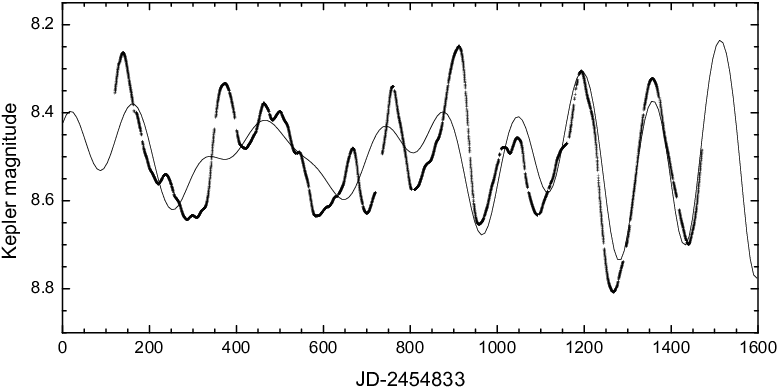
The Kepler light curve looks irregular (see Fig. 8) but the amplitude is quite large. Typical variations are in the general range of 0.3 magnitudes with variations just over 0.5 magnitudes for the full light curve. Autocorrelation analysis suggests a weakly correlated period of about 150 days. Fourier analysis of the data set gives two periods very close together: 156.52 d (P1) and 158.90 d (P2). Adding a variation on a time scale of about one year (P3) reproduces some aspects of the light curve including the correct prediction of most of the maximum and minimum times. However, much of the shape is not properly reproduced. No clear periodicity is visible in the residuals after subtracting P1 to P3. The double maximum structure reported by Zverev & Makarenko [81] is not seen in the Kepler data. Instead, the brightness of the maxima and minima seems to change in an irregular way. Similarly we do not see a 259 d period. The residuals O-C over the time span of our Kepler observations suggest a tendency towards an increasing period.

IV.3 V588 Lyr (KID 5614021)

Dahlmark [12] identified V588 Lyr as a possible Mira of period 221 days and a range from 12.5 magnitudes to 14.0 magnitudes. The GCVS lists V588 Lyr as an SRa variable. ASAS observations found it to be aperiodic with no clear light curve shape at the time of observation.

The Kepler light curve of V588 Lyr (Fig. 9) shows strong oscillations covering slightly over 1.1 Kepler magnitude of variation with individual maxima and minima levels varying considerably from cycle to cycle. During the time of observation the maxima and minima had alternate bright and faint cycles. The combination of two periods resulting from a Fourier analysis, P1(116.39 d) and P2 (217.93 d), permits a fit to the alternating depths, and the autocorrelation analysis agrees with these periods with even peaks more strongly correlated than the odd peaks. The addition of P3 (198.33 d) slightly improves the result but a few maxima/minima are not well reproduced. The residuals do not suggest the presence of an additional long period trend or further short periods, but rather non-sinusoidal variations and additional cycle-to-cycle irregularities. P2 is almost identical to the value given by Dahlmark [12].

IV.4 V1670 Cyg (KID 6127083)

Hoffleit and Sands [57] classified V1670 Cyg as an SR star with a period of 187.5 days. Dahlmark [12] rediscovered V1670 Cyg classifying it as a 191 day Mira with a visual magnitude ranging from 12.4 – 15.0. ASAS found V1670 Cyg to be quasi-periodic with a period of 193 days and visual amplitude of 1.99 magnitudes.

The light change observed by Kepler (Fig. 10) is very regular except for a very bright maximum at the beginning of the time series and a second bright maximum shortly before the end of our time series. There are variations in the depth of the minima from cycle to cycle. Autocorrelation indicates a strong correlation at a period of 187.5 days. Fourier analysis gives a single period of 187.19 d (P1), consistent with the autocorrelation analysis. Subtracting P1 from the light curve reveals a further, rather regular change corresponding to P2 (94.01 d) which is very close to half of P1. No further periodicity was found in the residuals. P1 is in nice agreement with the literature values for the period.

IV.5 V1766 Cyg (KID 7842386)

Huruhata [27] found V1766 Cyg to be a fairly regular SRa variable with a period of 119 days and a visual light range between 10.3 and 11.5 magnitudes. V1766 is classified as an MS star [65]. Based on infrared colors Wang and Chen [72] suggests that V1766 Cyg is an extrinsic S-star, i.e. its enrichment in s-process elements results from mass transfer from a more massive companion. ASAS lists the star as quasi-periodic with a period of 113.7 days and a visual amplitude of 0.80 mags.

In this case, periodicity is not very strongly expressed in the Kepler light curve (Fig. 11). Typical variations are generally in the range of 0.2 magnitudes with variations just over 0.4 magnitudes for the full light curve. Autocorrelation analysis suggests periods of 111 d and 120 d with only moderate to weak correlation. The Fourier diagram shows several peaks around 100 days period, a combination of 122.25 d (P1) and 104.21 d (P3) reproduces at least some features of the light curve. They are close to the ASAS value of 113.7 d. Double maxima are present, so we suspect that variations on a somewhat shorter time scale are present but they do not show up clearly in the Fourier diagram. A long time trend, which we fit with a period of 754 d (P2), seems to be present as well.

IV.6 V1253 Cyg (KID 8748160)

Dahlmark [12] found an uncertain period for V1253 Cyg of 188 to 226 days with a $V$ magnitude range of 11.8 to less than 15th and provided a a classification of SR. Pigulski et al. [52] list the star as quasi-periodic with a period of 187 days.

The Kepler light curve (Fig. 12) shows the brightness of the maxima and minima vary smoothly with time and a bump on the ascending branch. The data set is somewhat shorter than the others covering quarters Q6 through Q15. Autocorrelation suggests a strong correlation with a period of 196.5 d. Using Fourier analysis the times of maxima and minima can be reproduced very well with a single period of 197.15 d (P1). The changing maximum and minimum brightness and the bump can be qualitatively reproduced by adding a long period of 857.39 d (P2) and 99.35 d (P3). P2 is, of course, very poorly defined due to the limited length of the Kepler time series. P1 is not very far off the GCVS value. P3 is approximately half the period length of P1. Its S/N in the Fourier spectrum is only 2.

IV.7 AF Cyg (KID 9528112)

Fleming [15] noted that the bright (7.4 – 9.4 mag) M5 star now referred to as AF Cyg was variable. The spectral type at maximum light was confirmed M 5 III by Keenan [30]. The variability has been extensively studied over the last 100 years. The principal period is $\sim$ 93 d. Houk [26] first commented on the long secondary period (LSP) of 960 days. Using AAVSO data Mattei et al. [42] found periods of 92.9 and 165.9 d. An analysis of four sets of visual observations by Kiss et al. [35] confirmed the periods of 93 and 163 d and also confirmed a LSP of 921 d. The GCVS lists periods of 92.5, 175.8, and 941.2 days. Andronov & Chinarova [1] discuss the instabilities observed in the historic light curve. These include alternating dominance of the 93 and 176 d periods, intervals of regularly strong–weak maxima, and variations in times of the 93 day maximum from 79.4 to 97.4 d. For the data analyzed they found a dominant 94.2 d period with clusters of other periods present. Hinkle et al. [24] observed AF Cyg spectroscopically and derived an ‘orbital’ period of 926 $\pm$ 36 d matching the LSP. However, they note that the orbits for all LSP systems look the same so the motion is likely not orbital in origin. Glass & van Leeuwen [21] provide a parallax of 4.53 $\pm$ 0.64 mas which allows rough placement on a period luminosity diagram.

The Kepler light curve of AF Cyg (Fig. 13) shows a non-strict alternation of strong and weak maxima that could be interpreted as secondary maxima. The lack of a strict periodicity of this phenomenon suggests that instead this is an interplay of two excited periods of comparable amplitude with a period ratio close to an integer value. Several minor bumps are also present in particular on the descending part of the light curve. The light curve appears to have a long time variation exceeding the length of our monitoring. The typical amplitude of the light change is 0.5 mag in the Kepmag system.

A Fourier analysis reveals 4 main periods, and their combination gives a reasonable fit of the Kepler light curve although some deviations remain. The short term variability is accounted for by P1 (177.4 d) and P3 (93.6)̣. These two periods show a ratio close to 2, and thus agree with the above mentioned suspicion on the origin for the alternating bright and weak maxima. The long time change is represented by a period of 1867 d (P2). While P2 is a strong contributor to the light curve it is not adequately sampled. A further significant improvement of the fit can be achieved by including a fourth period of 441.3 d. Similar length periods were seen in the test data and may be related to the Kepler year. Autocorrelation analysis contains significant structure indicating evidence of multiple periods that are beating against each other. The highest correlation occurs at roughly 186 days but there are clearly indications of other periods present. Increasing anti-correlation between 800-1000 days is consistent with the longer period of 1867 days shown in the Fourier analysis.

For AF Cyg, which has been very well studied from the ground, we note the agreement of the two well sampled Kepler short periods with the literature periods (93 and 176 d) and the disagreement of the poorly sampled Kepler long periods (441 and 1867 d) with the literature period (941 d). The 941 d period is not apparent in the Kepler data. A Fourier analysis on the residual light curve after the removal of P1 through P4 gives an unclear pattern of additional frequencies between 0 and 0.03 cycles per day (c/d) and no significant peaks for frequencies above 0.03 c/d.

IV.8 V2412 Cyg (KID 10034169)

The variability of V2412 Cyg was discovered in 2001 as a part of the MISAO Project [80] but the only additional information was a possible coincidence with NSVS 5651487 [77]. NSVS 5651487 has a light curve with an $\sim$ 250 day period. ASAS [52] lists V2412 Cyg as aperiodic. The GCVS lists a 250 day period for the star and an SR: classification.

The Kepler time series for V2412 Cyg is not continuous (see Fig. 14). This star was observed from quarter Q2 through quarter Q6, then again during quarters Q8 and Q9, and finally in quarter Q14. In part the gaps are due to the placement of V2412 Cyg on the failed Kepler Module 3. The large gaps make it extremely difficult to determine an accurate flux level after each of these gaps. The behavior during the five continuous quarters gives us some clues to the proper treatment for this star. During these quarters we have strong oscillations covering over 1.5 Kepler magnitudes. The shifts to adjust for discontinuities between these continuous quarters were relatively small. We assume that the corrections in flux for quarters Q8 and Q14 would also be relatively small and we leave them uncorrected.

Times of maxima and minima can be reproduced reasonably well using one period of 255.91 d (P1) only. Variations in the brightness of the maxima and minima can be fitted nicely using a beat period of 241.19 d (P2). A third period of 140.42 d (P3) comes with a somewhat low S/N ratio, but including it helps to reduce the residuals significantly. The light curve shows an asymmetric oscillation with a steeper descent into minima than the rise to maxima and a slight bump in the ascending side which seems to shift its position from cycle to cycle. Including period P3 partly compensates for these bumps in the rising branches although some difference remains. Unfortunately an enticing wiggle in the ascending side during quarter Q14 $(\mbox{JD}-2454833\approx 1325)$ is cut off before the star reaches maximum sometime during the missing quarter Q15. P1 and P2 are both close to the GCVS value of 250 days.

IV.9 V1953 Cyg (KID 12215566)

Geßner [19] found that V1953 Cyg had slow semiregular variations with a photographic amplitude of 14.8-15.6 mag and a period of $\sim$ 150 days. The GCVS classifies V1953 Cyg as an SRb. The ASAS observations of V1953 Cyg list the star as quasi-periodic with a period of 95.2 days.

Although the Kepler measured light curve for V1953 Cyg (Fig. 15) looks quite irregular with a typical full amplitude of 0.4 mag, a combination of only three periods of 163.07 d (P1), 847.51 d (P2), and 93.41 d (P3) permits a fit to its main shape. P2 is poorly defined. Many details of the light curve, however, cannot be reproduced properly. A Fourier analysis on the residuals gives a number of peaks of similar amplitude between 500 and 50 days. Autocorrelation analysis finds a moderately correlated period of 179.5 days, but the correlation decays rapidly indicating that no single period dominates the light curve signal. P3 is similar to the ASAS period. P1 may be identical to the 150 d variation seen by Geßner [19].

V DISCUSSION

The Kepler data provide a new way to explore AGB pulsation through continuous, high-precision, photometric time-series spanning multiple years without significant interruption. Diurnal and seasonal effects in ground-based data result in time series that are too short or too fragmented for proper handling of the complex variability patterns observed in stars with very long periods [31, e.g.]. We were interested in exploring the various radial modes involved in SR pulsation, looking for long secondary periods, and searching for the existence of any low amplitude, short period events or pulsations. For the latter goal we were especially interested in looking for any periods that might be attributable to non-radial pulsations.

The Kepler data, of course, have limitations. Interruptions of the Kepler time series observations occurred due to telescope rotation every three months. SR variables have periods of order months to years [56] and extracting periods longer than a Kepler quarter posed special challenges in data reduction. Linking the quarters is surprisingly complicated due to a number of effects that can introduce photometric errors and we have explored optimum and non-subjective techniques for the construction of light curves spanning the whole Kepler monitoring time span. Another unfortunate reality of Kepler data, impacting this paper as well as the planet search goal of the mission, is that most of the stars observed are moderately faint. As a consequence most of the variable stars are not among the best studied objects of their classes. In spite of these problems, we find good agreement with the main periods detected in the Kepler data and ground-based results including the ASAS data set (see Table 3). The differences appear to be astrophysical and we will discuss them below.

V.1 Physical origins of pulsation

Physical interpretation of the observed pulsational behavior of red giants has been a topic of research and debate for several decades. Recent results for low luminosity red giants, based also on Kepler data [5, 3, 22], suggest that solar-like oscillations are observed in these stars. For the red giants less luminous than the RGB-tip, three parallel P-L-sequences are detected [59] that can be interpreted as radial low overtone modes plus non-radial (l=1) and (l=2) p-modes [67]. Asteroseismology using short cadence Kepler data provided the possibility of identifying core helium burning red giants on the basis of frequency separation of gravity modes [6].

Above the RGB tip where the classical long period variables are found the pulsation behavior is different. In the more luminous stars with their larger light and velocity amplitudes, the role of non-radial modes for the observed (semi-)periodic behavior is expected to be comparably low [74, e.g.], although some recent results by Stello et al. [64] may initiate a new discussion on this question. Various observational studies, more recently by Banyai et al. [2] and Kiss and Bedding [34], have demonstrated the difference in the variability behavior between RGB stars and the more luminous AGB stars. As pointed out by Xiong and Deng [79], stability analysis of pulsation modes in red giants shows a change from higher overtone radial modes in low luminosity red variables to lower overtone radial modes in the more luminous ones. This is in agreement with observations from globular cluster giants [39]. Model calculations, in particular of Wood and collaborators [75, and references therein], find the variability of the more luminous stars dominated by radial modes that are self-excited rather than stochastically excited. Coupling between convection and oscillations has been identified as the most likely excitation mechanism [79]. Buchler et al. [9] find that irregular pulsations are driven by energy exchange between two nonadiabatic modes in a 2:1 resonance.

Pulsation models nicely reproduce the period-luminosity sequences of luminous red giants [60, e.g.] in terms of a sequence of the fundamental radial mode and several low order overtone modes. The only exception is sequence D, the long secondary periods, which we will discuss in more detail below. The observed amplitudes in our program stars place them in the group of luminous red variables. The periods and parallax of AF Cyg demonstrate this unambiguously [21]. Hence we will focus on radial pulsation modes in this paper. Wood and Olivier [75] find that strange modes may develop in red giants beside the normal radial modes, but that they are always damped and thus should not be visible beside the normal radial modes on the upper giant branch. However, they might affect the period shown by a radial mode.

V.2 Decomposition of the Light Curve

The Kepler light curves typically appear at first examination very complex. However, in all our stars the combination of two or three periods was sufficient to predict the times of maxima and minima correctly. The exception is BU Lyr where this is correct for only the second half of the Kepler data set. However, in most cases a single period was not sufficient. This implies, as others have concluded, that even behavior classified irregular is multiperiodic [38].

For the detailed fitting of the complex light change shapes we used a combination of several periods. The continuity and the high photometric precision lowered the noise level in the Fourier power spectra significantly compared with ground-based surveys. In some cases, the observed changes in amplitudes and period lengths could be traced reasonably well, while in other stars the large residuals remained after subtraction of three to four frequencies, just like in the case of stars well observed from the ground. This is in agreement with other studies that note an irregular component in the light curves [70].

The two independent period search methods we applied lead to very similar results for period fits to the light curve. The period detection is robust for up to four periods at the precision and time span of the Kepler data. There are differences between the periods detected in our study and values in the literature based on different data sets for the same star. To explore this further, we downloaded the ASAS data set for one of our stars, V1953 Cyg, from the ASAS website⁷⁷ 7 http://www.astrouw.edu.pl/asas/, January 2014..

We selected V1953 Cyg because its light curve is one of the most irregular ones in our sample. The fit produced using our Kepler derived periods can be used to model almost all maxima and minima in the ASAS data set correctly and the combination of three periods reproduces a remarkable fraction of the changes in amplitude and period length. Naturally, the photometric uncertainties of the ASAS measurements are much larger than those of the Kepler measurements. Therefore, it is not possible to test the quality of the fit of the artificial light curve with similar precision.

In the ASAS data base V1953 Cyg is listed with a period of 95.2 d although the phased light curve using this period shows considerable scatter. Our Fourier analysis of the same ASAS data gives a period of 95.1 d as the first peak. An analysis of the residuals results in a second period of 66.1 d. The third period is a long period with almost 600 d length. The Kepler data show a third peak at 93.4 d and a second peak at 847.5 d. There is no Fourier peak visible in the ASAS data at the prime 163.1 d Kepler peak. Attempting to fit the Kepler light curve using the three periods derived from the ASAS light curve does not result in a good fit.

We find that the periods derived for semiregular variables are always connected to the star’s behavior at a specific time interval but are not necessarily transferable to a different data set observed at a different time. To identify the dominant period(s) of an SR variable an analysis of several pieces of the light curve obtained in different years seems to be necessary.

V.3 Pulsation Mode and Multiple Periods in the Same Mode

Multiple periods in SR variables are known from ground-based data. The Kepler light curves of the SR variables provide extremely clear examples. The multiple periods are manifested in three ways. Most of the program stars have two pulsation modes present that are separated by roughly a factor of two (Table 3). Historical light curves show that the dominant mode can switch between the two excited modes [9]. In 30 – 50 % of stars a third long period that is $\sim$ 9 $\pm$ 4 times longer than the dominant period can also be present [73]. In addition, each of the two pulsation modes can be composed of multiple periods spanning a small range of values [9, 59]. The result is that for any given epoch the resulting light curve can appear irregular or quite periodic.

An excellent example is the SRa variable V1766 Cyg which is described in the literature as fairly regular with a period of 119 days [27]. This is the one star star in our program that does not have a second mode present. Nonetheless during the time of the Kepler observations the light curve appears to be fairly irregular. This is due to the presence of a number of periods spanning the range from 104 to 122 d. On the other hand, two stars in our sample had SR: or SRb classifications, V1253 Cyg and V2412 Cyg, which imply that historically the light curves have been irregular (or badly sampled). These stars do indeed have multiple modes/periods but during the interval of the Kepler observations light curves were quite regular.

Time variations in the periods of late-type stars pulsating in multiple modes are well known from comparisons of observed and average periods. Changes in the strengths of radial modes also are a feature of type II Cepheids and RV Tauri stars [53]. In these stars as well as in LPVs variations of this type have been attributed to chaotic processes [9]. Using combined sinusoid fits to the LPV light curves from space missions like Kepler or COROT with a limited number of periods will not result in vastly different insight over ground-based analysis of these objects but does produce more reliable secondary periods. A substantial collection of high precision data could form the basis for testing statistical models of interior processes in LPVs [9, see for example].

The ASAS catalog [52] of variable stars in the Kepler field lists a total of 947 variables. Of these approximately 43% are in the ASAS category QPER. The QPER category consists mainly of SR variables, many with short periods, although we find that some of our program stars are classified as APER. Miras make up another 6 percent of the ASAS catalog variables. Figure 16 shows the period distribution of the QPER and Mira classes. A period distribution is the projection of the period-luminosity diagram onto the period axis. We are unable to produce a period-luminosity diagram since the luminosities of the Kepler field stars are unknown. For most of the program stars the dominant period is around 200 days with a shorter period of around 100 days. The longer periods match the long period SR distribution which is shared by the Miras. The Miras are fundamental mode pulsators [63]. The figure suggests that for most, if not all, of the program stars the long period is a fundamental mode.

To explore the periodicity patterns detected in our semiregular variables the period ratios are shown on a Petersen diagram in Figure 17. The Petersen diagram sets the ratio of the longer to the shorter period in relation to the longer period [51]. This approach has become widely used for the study of large sets of LPV light curve data [73, 63, e.g.]. In our Figure 17 we see a clustering of data points at period ratios of 1.1 and around 1.8. The ratios with the very long periods have been excluded. We show the theoretical ratios from fundamental mode (P0) and low overtone mode pulsation models (Pn) given in Figure 4 of Wood et al. [73]. The period ratios around 1.8 fall between the theoretical sequences for fundamental to first overtone mode and first to third overtone mode, respectively. All our sample SRVs with the exception of V1766 Cyg are found in that region with a pair of periods. Our result is consistent with the Petersen diagram presented in [73] for long period variables in the LMC. In analogy to their result we conclude that most of the SRVs in our sample are fundamental mode pulsators which also have the first overtone mode excited.

The period ratios clustering around 1.1, i.e. pairs of periods very close together, are not the result of two different low order radial pulsation modes [63, cf.]. Soszyński et al. [59] detected that about 35 % of the LMC semiregular variables in the OGLE database show such a behavior. In analogy to similar observations found in RR Lyr stars and Cepheids, these authors attribute such periods to non-radial oscillations. However, non-radial oscillations of the size required for M giant SR variability would result in unrealistic distortions [74, 47]. Non-radial modes also are not expected to provide significant velocity variations Wood et al. [74]. In the case of AF Cyg the velocity amplitude is $\sim$ 5 km s^-1. Similar results are found for the related stellar sample presented by Lebzelter & Hinkle [37].

Bedding et al. [4], while excluding non-radial oscillations as the origin of multiperiodic behavior, pointed out that the clustering of peaks in the Fourier power spectra of some LPVs has a striking similarity to the power spectra seen for stochastically excited pulsators like our sun. These are peaks from the same pulsation mode but with slightly different periods. However, Buchler et al. [9] point out that the low mass and high luminosity of AGB stars rules out a stochastic origin and favored chaotic pulsation dynamics arising from nonlinear interaction between two resonant pulsation modes. The light curves show that these peaks can co-exist or come and go without changing the overall brightness. Fox & Wood [16] noted a possible connection to convection. This has been discussed by Buchler et al. [9], Xiong and Deng [79] and most recently by Soszyński & Wood [62]. Soszyński & Wood [62] note that convection carries most of the energy through most of the envelope but is poorly modeled resulting in large computational uncertainties.

V.4 Long Secondary Period

As noted in the introduction the SR variables exhibit long secondary period (LSP) variations which have periods longer than the fundamental and typically $\sim$ 8 – 10 times longer than the dominant pulsation period [47]. While these long periods have been known for a long time [26, and references therein], LSP became an astrophysical problem when Wood et al. [73] identified period-luminosity sequences covering fundamental and overtone radial modes, as well as an LSP sequence, in MACHO observations of LMC AGB stars. Stars with LSP are multimode pulsators with a low overtone pulsation. In the AGB stars these are SR variables.

Recent surveys of luminous red giants by Soszyński et al. [60] and Fraser et al. [17] show that LSP is common. Soszyński et al. [60] suggests very low amplitude LSPs exist in up to 50% of variable AGB stars. The Kepler mission proved too brief to reliably measure LSP for any star. However, in agreement with Soszyński et al. [60] about half of our light curve fits require a long period of a few hundred days length. In the case of V1953 Cyg an LSP of $\sim$ 600 d is detectable from ground-based data. We tentatively identify LSPs of 800+ days for this star and 700+ days and 800+ days for V1766 Cyg and V1253 Cyg, respectively. These stars appear indistinguishable from the other SRVs in terms of global parameters like color. Among the SRVs with a long period in our sample, only one (V1766 Cyg) shows in addition a pair of periods of very similar length (104 and 122 days). The other four stars with such pairs of periods do not show an LSP, however, three of them show a third period about half the length of the two similar periods. The third period of BU Lyr is approximately two times larger than its pair of periods.

AF Cyg is well known from ground based observations to have a LSP [26]. In our data it shows an interesting characteristic of LSP not previously reported. The ground based LSP is $\sim$ 960 d which is also seen spectroscopically [24]. However we can not fit, even by attempting to force a fit by hand, this period to the Kepler data. On the other hand a period of roughly half the LSP is present. In the few stars where the LSP has been monitored spectroscopically the LSP is never the dominant photometric signal but is the dominant spectroscopic signal [24, 25]. Archival photometry of these stars suggests that the LSP can at times be difficult to observe.

The physical cause of LSPs remains unknown [47]. No clear non-radial modes were detected in our data in agreement with the previous discussion. Other investigators have excluded a number of other causes with remaining explanations including star spots [74] and long-period convective cycles [66]. Long-period convective cycles were mentioned as a possible cause discussed above for multiple periods in overtone modes. The requirement of dual mode pulsation for a long period suggests that the mode switching mechanism is involved with the long period. Coupling between convection and oscillation in SR pulsation has been invoked by both Buchler et al. [9] and Xiong and Deng [79]

The large amplitude LPV variables are Miras and these have been proven to be fundamental single-mode variables [63]. Soszyński et al. [63] also find that most SRVs are double mode variables with the fundamental mode and first overtone simultaneously excited. Our data similarly show most SRVs pulsating in two modes. As discussed in Soszyński & Wood [62] AGB stars evolve through instability stages from overtone mode pulsation to fundamental mode pulsation as the luminosity increases. The Miras in the LMC sample investigated by Wood et al. [73], Soszyński et al. [63] and others are single-mode variables and do not have an LSP. Since the SR class contains fundamental mode pulsators, the implication is that either LSP behavior limits the amplitude of pulsation or that a large pulsation amplitude somehow excludes LSP. Both explanations require that LSPs are an intrinsic feature of an AGB star related to overtone pulsation. This agrees with the conclusion reached by Wood & Nicholls [76] using other lines of evidence.

V.5 Very short period variations in LPVs

The 30 minute sample interval of the Kepler observations permits a search for rapid outbursts or very short time variations that have been discussed for LPVs on the basis of Hipparcos data [13]. A detailed search by eye of the program star Kepler light curves for such outbursts lasting between hours to a few days did not result in any detections. The time around the transition between two quarters was excluded. This result adds to other recent studies of this phenomenon that also did not detect such variations [36, 78]. We support the conclusion of these works that outbursts of duration less than a day in long period variables are very rare events.

VI CONCLUSIONS

Kepler data requires considerable care in reduction when used for multi-year high precision photometry. The technical problems have been discussed at length and solutions are presented. The resulting light curves of the SR variables are remarkably featureless at high time resolution and high precision. No variations were detected on ‘rapid’ time scales of one day or shorter. We have undertaken various types of period analysis on the data. While many of the light curves appear irregular the analysis shows this to be the result of combining two or three regular periods, suggesting that even the most irregular late-type variables are multiperiodic SR variables.

Multiperiodicity is a ubiquitous property of the SR variables that we analyzed. Using a Petersen diagram the SR variables in the current sample can be shown to be fundamental plus first overtone multimode radial pulsators. The multiple periods of the program stars are not solely the result of pulsation in more than one mode. These stars are in fact multiperiodic in three ways: They are generally pulsating in both the fundamental and an overtone mode. They have multiple periods in the dominant pulsation mode. Approximately half of the stars also have a long secondary period 8 to 10 times the length of the dominant pulsation period. The strong connection between LSP and multimode overtone pulsation suggests that LSP is related to the convective processes that drive mode switching and multiperiod modes in SR variables.

One of our goals was to use Kepler data to compare the different subclasses of SR variables. All the sample stars are multiperiodic with no apparent differences between the SRa, SRb, or SR: subclasses. We interpret the apparent regularity of some light curves as the result of constructive interference between beating periods. The implication, which is not surprising, is that the SR classification scheme is very insensitive to the location of a variable in the P-L diagram. When Gaia data becomes available it will be possible to place the Milky Way LPVs on the P-L diagram. Mira variables have been separated from the SR variable by pulsation amplitude but are also single mode pulsators. Previously SR variables have been seen as simply low amplitude versions of the fundamental mode mira pulsators [23] but this is clearly an incomplete description. It will be of interest to see how the extensively studied late-type variables fit on a P-L diagram where multimode versus single mode and large amplitude versus small amplitude variables can be compared.

The work of TL has been supported by the Austrian Science Fund under project number P23737-N16. EH thanks Mark Taylor for STILTS support. We wish to thank Steve Howell for his helpful comments and for providing the Mayall 4 m spectra. We also thank the Kitt Peak directors for their allocations of time on the Coude Feed telescope. Finally, we acknowledge the undergraduate students at SCSU who participated in the initial analysis of the Kepler data. Support to SCSU was provided through the NSF PAARE award AST-0750814 and NASA Kepler awards NNX11AB82G and NNX13AC24G. The National Optical Astronomy Observatory is operated by the Association of Universities for Research in Astronomy (AURA) under cooperative agreement with the National Science Foundation.

References

[1] Andronov, I.L. & Chinarova, L.L. 2012, arXiv:1212.6708
[2] Banyai, E., Kiss, L.L., Bedding, T.R., et al. 2013, MNRAS, 436, 1576
[3] Beck, P.G., Bedding, T.R., Mosser, B., et al. 2011, Science, 332, 205
[4] Bedding, T.R., Kiss, L.L., Kjeldsen, H., et al. 2005, MNRAS, 361, 1375
[5] Bedding, T.R., Huber, D., Stello, D., et al. 2010, ApJ, 713, L176
[6] Bedding, T.R., Mosser, B., Huber, D., et al. 2011, Nature, 471, 608
[7] Box, G.E.P., Jenkins, G.M. 1976, “Holden-Day Series in Time Series Analysis”, Revised ed., San Francisco: Holden-Day
[8] Bruntt, H., Grundahl, F., Tingley B., et al. 2003, A&A, 410, 323
[9] Buchler, J. R., Kolláth, Z., Cadmus, R. R. Jr. 2004, ApJ, 613, 532
[10] Caldwell, D.A., van Cleve, J.E., Jenkenis, J.M., et al. 2010, SPIE, 7731, 30
[11] Christensen-Dalsgaard, J., Kjeldsen, H., & Mattei, J.A. 2001, ApJ, 562, L141
[12] Dahlmark, L. 2000, IBVS, 4898, 1.
[13] de Laverny, P., Mennessier, M.O., Mignard, F., Mattei, J.A. 1998, A&A, 330, 169
[14] De Marchi, F., Poretti, E., Montalto, M., et al. 2007, A&A, 471, 515
[15] Fleming, W., & Pickering, E.C. 1910, Harvard Obs. Circular 158, 1
[16] Fox, M.W. & Wood, P.R. 1982, ApJ, 259, 198
[17] Fraser, O. J., Hawley S. L., Cook K. H., 2008, AJ, 136, 1242
[18] Garcia, R.A., Hekker, S., Stello, D., et al. 2011, MNRAS, 414, L6
[19] Geßner, H. 1988, Mitt.Veränderliche Sterne, 11, 150.
[20] Glass, I.S. & Lloyd Evans, T. 1981, Nature, 291, 303
[21] Glass, I.S. & van Leeuwen, F. 2007, MNRAS, 378, 1543
[22] Hekker, S., Mazumdar, A. 2013, Proc. IAU Sym 301, eds. J.A. Guzik, W.J. Chaplin, G. Handler, A.Pigulski, p.325
[23] Hinkle, K.H., Lebzelter, T., Scharlach, W.W.G. 1997, AJ, 114, 2686
[24] Hinkle, K.H., Lebzelter, T., Joyce, R., & Fekel, F. 2002, AJ, 123, 1002
[25] Hinkle, K.H., Fekel, F.C., & Joyce, R.R. 2009, ApJ, 692, 1360
[26] Houk, N. 1963, AJ, 68, 253
[27] Huruhata, M. 1983, IBVS, 2400, 1.
[28] Ita, Y., Tababé, T., Matsunaga, N., et al. 2004, MNRAS, 347, 720
[29] Jacoby, G. H., Hunter, D. A. and Christian, C. A. 1984, ApJS, 56, 257
[30] Keenan, P.C. 1966 ApJS, 13, 333
[31] Kerschbaum, F., Lebzelter, T., Lazaro, C. 2001, A&A, 375, 527
[32] Kholopov, P.N. ed. 1985, General Catalogue of Variable Stars, 4th ed, (Moscow:Nauka)
[33] Kiss, L.L. & Bedding, T.R. 2003, MNRAS, 343, L79
[34] Kiss, L.L., Bedding, T.R. 2004, MNRAS, 347, L83
[35] Kiss, L.L., Szatmáry, K., Cadmus, R.R., Jr., Mattei, J.A. 1999, A&A, 346, 542
[36] Lebzelter, T. 2011, A&A, 530, A35
[37] Lebzelter, T., Hinkle, K.H. 2002, A&A, 393, 563
[38] Lebzelter, T. & Obbrugger, M. 2009, AN, 330, 390
[39] Lebzelter, T., & Wood, P.R. 2005, A&A, 441, 1117
[40] Lebzelter, T., Schultheis, M., & Melchior, A.L. 2002, A&A, 393, 573
[41] Lenz, P., Breger, M. 2005, CoAst, 146, 53
[42] Mattei, J. A., Foster, G., Hurwitz, L. A., Malatesta, K. H., Willson, L. A., & Mennessier, M. O. 1997, in Hipparcos Venice ’97, ed. B. Battrick (ESA SP-402) (ESA: Noordwijk), 269
[43] Miller, W. 1969, Ricerche Astronomiche, 7, 459.
[44] Mochejska, B., Stanek, K., & Kaluzny, J. 2003, AJ, 125, 3175
[45] Mochejska, B., Stanek, K., Sasselov, D. et al. 2005, AJ, 129, 2856
[46] Neugebauer, G., Leighton, R.B. 1969, “Two-micron Sky Survey”, NASA SP-3047 (Washington:NASA)
[47] Nicholls, C.P., Wood, P.R., Cioni, M.-R. L., & Soszyński, I. 2009, MNRAS, 399, 2063
[48] Percy, J. R. 2007, Understanding Variable Stars (Cambridge: Cambridge Univ. Press), Chapter 6, p. 167
[49] Percy, J.R., Esteves, S., Lin, A., et al. 2009, JAVSO, 37, 71
[50] Percy, J. & Mohammed, F. 2004, JAVSO, 32, 9
[51] Petersen, J.O. 1973, A&A, 27, 89
[52] Pigulski, A., Pojmanski, G., Pilecki, B., Szczygiel, D. 2009, Acta Astronomica, 59, 33
[53] Pollard, K. R., Alcock, C., Allsman, R. A. et al. 2000, in IAU Coll. 176 “The Impact of Large-Scale Surveys on Pulsating Star Research”, eds. L. Szabados & D. Kurtz., ASP Conference Series, 203, 89
[54] Preston, G., Krzeminski, W., Smak, J., Williams, J. 1963, ApJ, 137, 401
[55] Ross, F. 1928, AJ, 38, 144
[56] Samus N.N., Durlevich O.V., Kazarovets E V., et al., 2007-2012, General Catalogue of Variable Stars, VizieR Online Data Catalog
[57] Sands, S. 1978, JAVSO, 7, 79
[58] Smith, J.C., Stumpe, M.C., Van Cleve, J.E., et al. 2012, PASP, 124, 1000
[59] Soszyński, I., Udalski, A., Kubiak, M., et al. 2004, Acta Astronomica, 54, 129
[60] Soszyński, I., Dziembowski, W. A., Udalski, A., et al. 2007, Acta Astronomica, 57, 201
[61] Soszyński, I., et al., 2009, Acta Astron., 59, 239
[62] Soszyński, I. & Wood, P.R. 2013, ApJ, 763, 103
[63] Soszyński, I., Wood, P.R., Udalski, A. 2013, ApJ, 779, 167
[64] Stello, D., Compton, D.L., Bedding, T., et al. 2014, ApJ, 788, L10
[65] Stephenson, C.B. 1984, PW&SO, 3, 1
[66] Stothers, R.B. 2010, ApJ, 725, 1170
[67] Takayama, M., Saio, H., Ita, Y. 2013, MNRAS, 431, 3189
[68] Templeton, M. 2004, JAVSO, 32, 41
[69] Tokunaga, A.T. 2000, in “Astrophysical Quantities” A.N. Cox ed. (Springer-Verlag:New York), p. 152
[70] Turner, D.G., Berdnikov, L.N., Percy, J.R., Abdel-Sabour Abdel-Latif, M. 2010, Odessa Astronomical Publications, 23, 129
[71] Wahlgren, G. 1992, AJ, 104, 1174
[72] Wang, X.H., Chen, P.S. 2002, A&A, 387, 129
[73] Wood, P.R., Alcock, C., Allsman, R.A., et al. 1999, in “Asymptotic Giant Branch Stars”, T. Le Bertre, A. Lèbre, & C. Waelkens eds. Proc. IAU Symposium 191, 151
[74] Wood, P.R., Olivier, E.A., Kawaler, S.D. 2004, ApJ, 604, 800
[75] Wood, P.R., Olivier, E.A. 2014, MNRAS, 440, 2576
[76] Wood, P.R. & Nicholls, C.P. 2009, ApJ, 707, 573
[77] Woźniak, P.R., Vestrand, W.T., Akerlof, C.W., et al. 2004a, AJ, 127, 2436
[78] Woźniak, P.R., McGowan, K.E., Vestrand, W.T. 2004b, ApJ, 610, 1038
[79] Xiong, D.R., Deng, L. 2007, MNRAS, 378, 1270
[80] Yoshida, S., Ohkura, N., Kadota, K., 2004, Misao Project Variable Stars Catalogue (www.aerith.net/misao/public/MisV.dat)
[81] Zverev, M.S. & Makarenko, E.N. 1979, Premennye Zvezdy Prilozhenie (Variable Stars, Supplement), 3, No. 17, 431