CAPRI: Efficient Inference of Cancer Progression Models from Cross-sectional Data
Abstract
We devise a novel inference algorithm to effectively solve the cancer progression model reconstruction problem. Our empirical analysis of the accuracy and convergence rate of our algorithm, CAncer PRogression Inference (CAPRI), shows that it outperforms the state-of-the-art algorithms addressing similar problems.
Motivation:
Several cancer-related genomic data have become available (e.g., The Cancer Genome Atlas, TCGA) typically involving hundreds of patients. At present, most of these data are aggregated in a cross-sectional fashion providing all measurements at the time of diagnosis.
Our goal is to infer cancer “progression” models from such data. These models are represented as directed acyclic graphs (DAGs) of collections of “selectivity” relations, where a mutation in a gene A “selects” for a later mutation in a gene B. Gaining insight into the structure of such progressions has the potential to improve both the stratification of patients and personalized therapy choices.
Results:
The CAPRI algorithm relies on a scoring method based on a probabilistic theory developed by Suppes, coupled with bootstrap and maximum likelihood inference. The resulting algorithm is efficient, achieves high accuracy, and has good complexity, also, in terms of convergence properties. CAPRI performs especially well in the presence of noise in the data, and with limited sample sizes. Moreover CAPRI, in contrast to other approaches, robustly reconstructs different types of confluent trajectories despite irregularities in the data.
We also report on an ongoing investigation using CAPRI to study atypical Chronic Myeloid Leukemia, in which we uncovered non trivial selectivity relations and exclusivity patterns among key genomic events.
Availability:
CAPRI is part of the TRanslational ONCOlogy R package and is
freely available on the web at:
http://bimib.disco.unimib.it/index.php/Tronco
Contact:
daniele.ramazzotti@disco.unimib.itdaniele.ramazzotti@disco.unimib.it
1 Introduction
Analysis and interpretation of the fast-growing biological data sets that are currently being curated from laboratories all over the world require sophisticated computational and statistical methods.
Motivated by the availability of genetic patient data, we focus on the problem of reconstructing progression models of cancer. In particular, we aim to infer the plausible sequences of genomic alterations that, by a process of accumulation, selectively make a tumor fitter to survive, expand and diffuse (i.e., metastasize). Along the trajectories of progression, a tumor (monotonically) acquires or “activates” mutations in the genome, which, in turn, produce progressively more “viable” clonal subpopulations over the so-called cancer evolutionary landscape (cfr., [1, 2, 3]).
Knowledge of such progression models is very important for drug development and in therapeutic decisions. For example, it has been known that for the same cancer type, patients in different stages of different progressions respond differently to different treatments.
Several datasets are currently available that aggregate diverse cancer-patient data and report in-depth mutational profiles, including e.g., structural changes (e.g., inversions, translocations, copy-number variations) or somatic mutations (e.g., point mutations, insertions, deletions, etc.). An example of such a dataset is The Cancer Genome Atlas (TCGA) (cfr., [4])). These data, by their very nature, only give a snapshot of a given tumor sample, mostly from biopsies of untreated tumor samples at the time of diagnoses. It still remains impractical to track the tumor progression in any single patient over time, thus limiting most analysis methods to work with cross-sectional data11 1 Unlike longitudinal studies, these cross-sectional data are derived from samples that are collected at unknown time points, and can be considered as “static”..
To rephrase, we focus on the problem of cancer progression models reconstruction from cross-sectional data. The problem is not new and, to the best of our knowledge, two threads of research starting in the late 90’s have addressed it. The first category of works examined mostly gene-expression data to reconstruct the temporal ordering of samples (cfr., [5, 6]). The second category of works looked at inferring cancer progression models of increasing model-complexity, starting from the simplest tree models (cfr. [7]) to more complex graph models (cfr., [8]); see the next subsection for an overview of the state of the art. Building on our previous work described in [9] we present a novel and comprehensive algorithm of the second category that addresses this problem.

The new algorithm proposed here is called CAncer PRogression Inference (CAPRI) and is part of the TRanslational ONCOlogy (TRONCO) package (cfr., [10]). Starting from cross-sectional genomic data, CAPRI reconstructs a probabilistic progression model by inferring “selectivity relations”, where a mutation in a gene A “selects” for a later mutation in a gene B. These relations are depicted in a combinatorial graph and resemble the way a mutation exploits its “selective advantage” to allow its host cells to expand clonally. Among other things, a selectivity relation implies a putatively invariant temporal structure among the genomic alterations (i.e., events) in a specific cancer type. In addition, these relations are expected to also imply “probability raising” for a pair of events in the following sense: Namely, a selectivity relation between a pair of events here signifies that the presence of the earlier genomic alteration (i.e., the upstream event) that is advantageous in a Darwinian competition scenario increases the probability with which a subsequent advantageous genomic alteration (i.e., the downstream event) appears in the clonal evolution of the tumor. Thus the selectivity relation captures the effects of the evolutionary processes, and not just correlations among the events and imputed clocks associated with them. As an example, we show in (Figure 1) the selectivity relation connecting a mutation of egfr to the mutation of cdk.
Consequently, an inferred selectivity relation suggests mutational profiles in which certain samples (early-stage patients) display specific alterations only (e.g., the alteration characterizing the beginning of the progression), while certain other samples (e.g., late-stage patients) display a superset subsuming the early mutations (as well as alterations that occur subsequently in the progression).
Various kinds of genomic aberrations are suitable as input data, and include somatic point/indel mutations, copy-number alterations, etc., provided that they are persistent, i.e., once an alteration is acquired no other genomic event can restore the cell to the non-mutated (i.e., wild type) condition22 2 For instance, epigenetic alterations such as methylation and alterations in gene expression are not directly usable as input data for the algorithm. Notice that the selection of the relevant events is beyond the scope of this work and requires a further upstream pipeline, such as that provided, for instance, in [11, 3]..
The selectivity relations that CAPRI reconstructs are ranked and subsequently further refined by means of a hybrid algorithm, which reasons over time, mechanism and chance, as follows. CAPRI’s overall scoring methods combine topological constraints grounded on Patrick Suppes’ conditions of probabilistic causation (see e.g., [12]), with a maximum likelihood-fit procedure (cfr., [13]) and derives much of its statistical power from the application of bootstrap procedures (see e.g., [14]). CAPRI returns a graphical model of a complex selectivity relation among events which captures the essential aspects of cancer evolution: branches, confluences and independent progressions. In the specific case of confluences, CAPRI’s ability to infer them is related to the complexity of the “patterns” they exhibit, expressed in a logical fashion. As pointed out by other approaches (cfr., [15]), this strategy requires trading off complexity for expressivity of the inferred models, and results in two execution modes for the algorithm: supervised and unsupervised, which we discuss in details in Sections 2 and 3.
In Section 3 (Methods) we show that CAPRI enjoys a set of attractive properties in terms of its complexity, soundness and expressivity, even in the presence of uniform noise in the input data – e.g., due to genetic heterogeneity and experimental errors. Although many other approaches enjoy similar asymptotic properties, we show that CAPRI can compute accurate results with surprisingly small sample sizes (cfr., Section 4). Moreover, to the best of our knowledge, based on extensive synthetic data simulations, CAPRI outperforms all the competing procedures with respect to all desirable performance metrics. We conclude by showing an application of CAPRI to reconstruct a progression model for atypical Chronic Myeloid Leukemia (aCML) using a recent exome sequencing dataset, first presented in [16].
1.1 State of the Art
For an extensive review on cancer progression model reconstruction we refer to the recent survey by [17]. In brief, progression models for cancer have been studied starting with the seminal work of [18] where, for the first time, cancer progression was described in terms of a directed path by assuming the existence of a unique and most likely temporal order of genetic mutations. [18] manually created a (colorectal) cancer progression from a genetic and clinical point of view. More rigorous and complex algorithmic and statistical automated approaches have appeared subsequently. As stated already, the earliest thread of research simply sought more generic progression models that could assume tree-like structures. The oncogenetic tree model captured evolutionary branches of mutations (cfr., [7, 19]) by optimizing a correlation-based score. Another popular approach to reconstruct tree structures appears in [20]. Other general Markov chain models such as, e.g., [21] reconstruct more flexible probabilistic networks, despite a computationally expensive parameter estimation. In [9], we introduced an algorithm called CAncer PRogression Extraction with Single Edges (CAPRESE), which, based on its extensive empirical analysis, may be deemed as the current state-of-the-art algorithm for the inference of tree models of cancer progression. It is based on a shrinkage-like statistical estimation, grounded in a general theoretical framework, which we extend further in this paper. Other results that extend tree representations of cancer evolution exploit mixture tree models, i.e., multiple oncogenetic trees, each of which can independently result in cancer development (cfr., [22]). In general, all these methods are capable of modeling diverging temporal orderings of events in terms of branches, although the possibility of converging evolutionary paths is precluded.
To overcome this limitation, the most recent approaches tends to adopt Bayesian graphical models, i.e., Bayesian Networks (BN). In the literature, there have been two initial families of methods aimed at inferring the structure of a BN from data (cfr., [13]). The first class of models seeks to explicitly capture all the conditional independence relations encoded in the edges and will be referred to as structural approaches; the methods in this family are inspired by the work on causal theories by Judea Pearl (cfr., [23, 24, 25, 26]). The second class – likelihood approaches – seeks a model that maximizes the likelihood of the data (cfr., [27, 28, 29]).
A more recent hybrid approach to learn a BN which combines the two families above by constraining the search space of the valid solutions and, then, fitting the model with likelihood maximization (see [15, 8, 30]). A further technique to reconstruct progression models from cross-sectional data was introduced in [31], in which the transition probabilities between genotypes are inferred by defining a Moran process that describes the evolutionary dynamics of mutation accumulation. In [32] this methodology was extended to account for pathway-based phenotypic alterations.
2 Approach
In what follows, we denote with and the observed marginal and conditional probability of an event, whose complement is denoted with the diacritical mark (macron).
A probabilistic model of selective advantage.
Central to CAPRI’s score function is Suppes’ notion of probabilistic causation (cfr., [12]), which can be stated in the following terms: a selectivity relation33 3 Suppes presents the relation in terms of causality; however, we avoid Suppes’ terminology as we build on just two of his many axioms, which only give rise to the notion of prima-facie causality. among two observables and if (1) occurs earlier than – temporal priority (tp) – and (2) if the probability of observing raises the probability of observing , i.e., – probability raising (pr). The definition of probability raising subsumes positive statistical dependency and mutuality (see, e.g., [9]). Note that the resulting relation (also, called prima facie causality) is purely observational and remains agnostic to the possible mechanistic cause-effect relation involving and .
While Suppes’ definition of probabilistic causation has known limitations in the context of general causality theory (see discussions in, e.g., [33, 34]), in the context of cancer evolution, this relation appropriately describes various features of selective advantage in somatic alterations that accumulate as tumor progresses.
Thus, in our framework, we implement the temporal priority among events – condition (1) – as , because it is intuitively sound to assume that the (cumulative) genomic events occurring earlier are the ones present in higher frequency in a dataset. In addition, condition (2) is implemented as is, that is by requiring that for each pair of observables and directly connected, is verified. Taken together, these conditions gives rise to a natural ordering relation among events, written “” and read as “ has a selective influence on .” This relation is a necessary but not sufficient condition to capture the notion of selective advantage, and additional constraints need to be imposed to filter spurious relations. Spurious correlations are both intrinsic to the definition (e.g., if then also , which could be spurious) and to the model we aim at inferring, because data is finite as well as corrupted by noise.
Building on this framework, we devise inference algorithms that capture the essential aspects of heterogeneous cancer progressions: branching, independence and convergence – all combining in a progression model.
| temporal priority | |
|---|---|
| path | |
| branch | and |
| temporal priority | |
| co-occurrence | and and |
Progression patterns.
The complexity of cancer requires modeling multiple non-trivial patterns of its progression: for a specific event, a pattern is defined as a specific combination of the closest upstream events that confers a selective advantage.
As an example, imagine a clonal subpopulation becoming fit – thus enjoying expansion and selection – once it acquires a mutation of gene , provided it also has previously acquired a mutation in a gene in the upstream / pathway. In terms of progression, we would like to capture the trajectories: and precedes (where denotes the absence of an event in the gene).
To establish this analysis formally, we augment our model of selection in a tumor with a language built from simple propositional logic formulas using the usual Boolean connectives: namely, “and” (), “or” () and “xor” (). These patterns can be described by formulæ in a propositional logical language, which can be rendered in Conjunctive Normal Form (CNF). A CNF formula has the following syntax: , where each is a disjunctive clause over a set of literals, each literal representing an event or its negation. Given this (rather obvious) pattern representation, we write the conditions for selectivity with patterns as
| (1) |
with respect to the example above, patterns 44 4 Note that the conjunction in our setting is interpreted differently from the classical notion (and the one adopted in e.g., [8]) since implies and in our framework. See also [17]. Moreover, note that the scope of this study is intentionally kept limited from further generalization of formulæ i.e., we will not consider statements of the form , where the rightmost argument is a formula too. could be and
In our framework the problem of reconstructing a probabilistic graphical model of progression reduces to the following: for each input event , assess a set of selectivity patterns , filter the spurious ones, and combine the rest in a direct acyclic graph (DAG)55 5 A DAG is formed by a set of nodes and oriented edges connecting one node to another, such that there are no directed loops among them. See SI Section 1 for a technical definition., augmented with logical symbols. Notice that while we broke down the progression extraction into a series of sub-tasks, the problem remains complex: patterns are unknown, potentially spurious, and exponential in formula size; data is noisy; patterns must allow for ‘‘imperfect regularities’’, rather than being strict66 6 This statement implies that there could be samples – i.e., patients – contradicting a pattern which still remains valid at a population level. For this reason a pattern is sometimes called a “noisy and”.. To summarize, in our setting we can model complex progression trajectories with branches (i.e., events involved in various patterns), independent progressions (i.e., events without common ancestors) and convergence (via CNF formulas). The framework we introduce here is highly versatile, and to the best of our knowledge, it infers and checks more complex claims than any cancer progression algorithms described thus far (cfr.,[7, 8, 9]).
3 Methods

Building on the framework described in the previous section, we now describe the implementation of CAPRI’s building blocks. Notice that, in general, the inference of cancer progression models requires a complex data processing pipeline, as summarized in Figure 3; its architecture optimally exploits CAPRI’s efficiency.
Assumptions.
CAPRI relies on the following assumptions: Every pattern is expressible as a propositional CNF formula; All events are persistent, i.e., an acquired mutation cannot disappear; All relevant events in tumor progression are observable, with the observations describing the progressive phenomenon in an essential manner (i.e., closed world assumption, in which all events ‘driving’ the progression are detectable); All the events have non-degenerate observed probability in ; All events are distinguishable, in the following sense: input alterations produce different profiles across input samples. Assumptions - relate to the framework derived in previous section, while imposes an onerous burden on the experimentalists, who must select the relevant genomic events to model77 7 Theoretically, this assumption - common to other Bayesian learning problems - is necessary to prove CAPRI’s ability to extract the exact model in the optimal case of infinite samples. Practically, as all relevant events are hardly selectable a priori and sample size is finite, further statistics can be used to select the most relevant driver alterations – see also Section 4, Results and Discussion. Nonetheless, CAPRI can provide significant results even if this assumption is not or cannot be verified.. Assumption relates instead to the statistical distinguishability of the input events (see the next section on CAPRI’s Data Input). .
Trading Complexity for Expressivity.
To automatically extract the patterns that underly a progression model, one may try to adopt a brute-force method of enumerating and testing all possibilities. This strategy is computationally intractable, however, since the number of (distinct) (sub)formulæ grows exponentially with the number of events included in the model. Therefore, we need to exploit certain properties of the relation whenever possible, and trade expressivity for complexity in other cases, as explained below.
Note that singleton and co-occurrence () types of patterns are amenable to compositional reasoning: if then, for any , . This observation leads to the following straightforward strategy of evaluating every conjunctive (and henceforth singleton) relation using a pairwise-test for the selectivity relation (see Figure 2).
Unfortunately, it is easy to see that this reasoning fails to generalize for CNF patterns: e.g., when the pattern contains disjunctive operators (). As an example, consider pattern , in a cancer where progression to is more prevalent than and . In this case, considering sub-formulas only we might find but miss because the probability of mutated is smaller than that of , thus invalidating condition of relation . Notice that in extreme situations, when the data is very noisy, the algorithm may even “invert” the selectivity relation to .
This difficulty is not a peculiarity of our framework, but rather intrinsic to the problem of extracting complex “causal networks” (cfr., [23, 24, 34]). To handle this situation, CAPRI adapts a strategy that trades complexity for expressivity: the resulting inference procedure, Algorithm 1, can be executed in two modes: unsupervised and supervised. In the former, inferred patterns of confluent progressions are constrained to co-occurrence types of relations, in the latter CAPRI can test more complex patterns, i.e., disjunctive or “mutual exclusive” ones, provided they are given as prior hypotheses. In both cases, CAPRI’s complexity – studied in next sections – is quadratic both in the number of events and hypotheses.
Data Input (Step 1).
CAPRI (cfr., Algorithm 1) requires an input set of events, i.e., genomic alterations, and cross-sectional samples, represented as a dataset in an binary matrix , in which an entry if the event was observed in sample , and otherwise. Assumption is satisfied when all columns in differ - i.e., the alteration profiles yield different observations.
Optionally, a set of input hypotheses , where each is a well-formed88 8 Formally, we require that , where represents the usual syntactical ordering relation among atomic events and formulas, and disallows for example . CNF formula. Note that we advise that the algorithm be used in the following regime 99 9 In the current biomedical setting, the number of samples () is usually in the hundreds, while number of possible mutations () and hypotheses (), absent any pre-processing, could be large, thus violating the assumption; in these cases, we rely on various commonly used pre-preprocessing filters to limit to driver mutations, and to simple hypotheses involving the driver mutations. However, in the future as the number of samples increases, we envision a more agnostic application. : .
Data Preprocessing (Lifting, step 2).
When input hypotheses are provided (e.g., by a domain expert), CAPRI first performs a lifting operation over to permit direct inference of complex selectivity relations over a joint representation, which involve input events as well as the hypotheses. Lifting operation evaluates each input CNF formula – for all input hypotheses in – and outputs a lifted matrix to be processed further as in step 1. As an example, consider hypothesis lifted input matrix is:
Note that the first row (profile ) contradicts the hypothesis, while all other rows support it.
Selectivity Topology (steps 3, 4, 5).
We exploit a compositional approach to test CNF hypotheses as follows: the disjunctive relations are grouped, and treated as if they were individual objects in . For example, when a formula where is considered, we assess as whether and hold – with the proviso that we treat as an individual event. Formally, with we denote the disjunctive clauses in a CNF formula.
Nodes in the reconstruction are all input events together with all the disjunctive clauses of each input formula .
Edges in the reconstructed DAG are patterns that satisfy both conditions (1) and (2) of the selectivity relation . Formally, CAPRI includes an edge between two nodes and only if both and are strictly positive. Note that can be both a disjunctive clause as well as a singleton event. A function assigns a parent to each node that is not an input formula. Note that this approach works efficiently by nature of the lifted representation of . The reconstructed DAG contains all the true positive patterns, with respect to , plus spurious instances of which CAPRI subsequently removes in step 6 (cfr., the Supplementary Material for a proof of this statement).
Note that can be readily interpreted as a probabilistic graphical model, once it is augmented with a labeling function , where is the set of nodes – i.e., the genetic alterations – such that is the independent probability of observing mutation in a sample, whenever all of its parent mutations (i.e., ) are observed (if any). Thus induces a distribution of observing a subset of events in a set of samples (i.e., a probability of observing a certain mutational profile in a patient).
Maximum Likelihood Fit (step 6).
As the selectivity relation provides only a necessary condition, we must filter out all of its spurious instances that might have been included in (i.e., the possible false positives).
For any selectivity structure, spurious claims contribute to a reduction in the likelihood-fit relative to true patterns. Thus, a standard maximum-likelihood fit can be used to select and prune the selectivity DAG (including a regularization term to avoid over-fitting1010 10 In principle other regularisation strategies common to Bayesian learning could be used, e.g., Akaike information criterion (see [29] and references therein). In this paper, we prefer to work with BIC which, in general, trades model complexity to reduce false positives rate.). Here, we adopt the Bayesian Information Criterion (BIC), which implements Occam’s razor by combining log-likelihood fit with a penalty criterion proportional to the of the DAG size via Schwarz Information Criterion (see [27]). The BIC score is defined as follows.
| (2) |
Here, is the lifted input matrix, denotes the number of samples and is the number of parameters in the model . Because, in general, depends on the number of parents each node has, it is a good metric for model complexity. Moreover, since each edge added to increases model complexity, the regularization term based on favors graphs with fewer edges and, more specifically, fewer parents for each node.
At the end of this step, and the labeling function are modified accordingly, based on the result of BIC regularization. By collecting all the incoming edges in a node it is possible to extract the patterns, which have been selected by CAPRI as the positive ones.
| (3) |
Inference Confidence: Bootstrap and Statistical Testing.
To infer confidence intervals of the selectivity relations , CAPRI employs bootstrap with rejection resampling as follows, by estimating a distribution of the marginal and joint probabilities. For each event, CAPRI samples with repetitions rows from the input matrix (bootstrapped dataset), CAPRI next estimates the distributions from the observed probabilities, and finally, CAPRI rejects values which do not satisfy and , and iterates restarting from . We stop when we have, for each distribution, at least values (in our case ). Any inequality (i.e., checking temporal priority and probability raising) is estimated using the non-parametric Mann-Whitney U test1212 12 The Mann-Whithney U test is a rank-based non-parametric statistical hypothesis test that can be used as an alternative to the Student’s t-test and is particularly useful if data are not normally distributed. with -values set to . We compute confidence -values for both temporal priority and probability raising using this test, which need not assume Gaussian distributions for the populations.
Once a DAG is inferred both parametric and non-parametric bootstrapping methods can be used to assign a confidence level to its respective pattern and to the overall model. Essentially, these tests consist of using the reconstructed model (in the parametric case), or the probabilities observed in the dataset (in the non-parametric case) to generate new synthetic datasets, which are then reused to reconstruct the progressions (see, e.g., [35] for an overview of these methods). The confidence is estimated by the number of times the DAG or any instance of is reconstructed from the generated data.
Complexity, Correctness and Expressivity.
CAPRI has the following asymptotic complexity (Theorem 1, SI Section 2):
Without input hypotheses the execution is self-contained and polynomial in the size of .
In addition to the above cost, CAPRI tests input hypotheses of at a polynomial cost in the size of . In this case, however, its complexity may range over many orders of magnitude depending on the structural complexity of the input set consisting of hypotheses.
An empirical analysis of the execution time of CAPRI and the competing techniques on synthetic datasets is provided in the SI, Section 3.5.
CAPRI is a sound and complete algorithm, and its expressivity in terms of the inferred patterns is proportional to the hypothesis set which, in turn, determines the complexity of the algorithm. With a proper set of input hypothesis, CAPRI can infer all (and only) the true patterns from the data, filtering out all the spurious ones (Theorem 2, SI Section 2).Without hypotheses, besides singleton and co-occurrence, no other patterns can be inferred (see Figure 2). Also, some of these claims might be spurious in general for more complex (and unverified) CNF formula (Theorem 3, SI Section 2).
4 Results and Discussion

To determine CAPRI’s relative accuracy (true-positives and false-negatives) and performance compared to the state-of-the-art techniques for network inference, we performed extensive simulation experiments. From a list of potential competitors of CAPRI, we selected: Incremental Association Markov Blanket (IAMB, [26]), the PC algorithm (see [25]), Bayesian Information Criterion (BIC, [27]), Bayesian Dirichlet with likelihood equivalence (BDE, [28]) Conjunctive Bayesian Networks (CBN, [8]) and Cancer Progression Inference with Single Edges (CAPRESE, [9]). These algorithms constitute a rich landscape of structural methods (IAMB and PC), likelihood scores (BIC and BDE) and hybrid approaches (CBN and CAPRESE).
Also, we applied CAPRI to the analysis of an atypical Chronic Myeloid Leukemia dataset of somatic mutations — with data based on [16].
4.1 Synthetic data
We performed extensive tests on a large number of synthetic datasets generated by randomly parametrized progression models with distinct key features, such as the presence/absence of: branches, confluences with patterns of co-occurrence, independent progressions (i.e., composed of disjoint sub-models involving distinct sets of events). Accordingly, we distinguish four classes of generative models with increasing complexity and the following features:
| trees | forests | connected DAGs | disconnected DAGs | |
| (1) | ✓ | ✓ | ✓ | ✓ |
| (2) | ✗ | ✗ | ✓ | ✓ |
| (3) | ✗ | ✓ | ✗ | ✓ |
The choice of these different type of topologies is not a mere technical exercise, but rather it is motivated, in our application of primary interest, by heterogeneity of cancer cell types and possibility of multiple cells of origin.
To account for biological noise and experimental errors in the data we introduce a parameter which represents the probability of each entry to be random in , thus representing a false positive () and a false negative rate (): . The noise level complicates the inference problem, since samples generated from such topologies will likely contain sets of mutations that are correlated but causally irrelevant.
To have reliable statistics in all the tests, distinct progression models per topology are generated and, for each model, for every chosen combination of sample set size and noise rate , different datasets are sampled (see SI Section 3 for our synthetic data generation methods).
Algorithmic performance was evaluated using the metrics Hamming distance (HD), precision and recall, as a function of dataset size, and . HD measures the structural similarity among the reconstructed progression and the generative model in terms of the minimum-cost sequence of node edit operations (inclusion and exclusion) that transforms the reconstructed topology into the generative one1313 13 This measure corresponds to the sum of false positives and false negative and, for a set of events, is bounded above by when the reconstructed topology contains all the false negatives and positives.. Precision and recall are defined as follows: precision = TP/(TP + FP) and recall = TP/(TP + FN), where TP are the true positives (number of correctly inferred true patterns), FP are the false positives (number of spurious patterns inferred) and FN are the false negatives (number of true patterns that are not inferred ). The closer both precision and recall are to , the better.
In Figure 4 we show the performance of CAPRI and of the competing techniques, in terms of Hamming distance, on datasets generated from models with events and all the four different topologies. In particular, we show the performance: in the case of noise-free datasets, i.e., and different values of the sample set size and in the case of a fixed sample set size, (size that is likely to be found in currently available cancer databases, such as TCGA (cfr., [4])) and different values of the noise rate . As is evident from Figure 4 CAPRI outperforms all the competing techniques with respect to all the topologies and all the possible combinations of noise rate and sample set size, in terms of average Hamming distance (with the only exception of CAPRESE in the case of tree and forests, which displays a behavior closer to CAPRI’s). The analyses on precision and recall display consistent results (SI Section 3). In other words, we demonstrate on the basis of extensive synthetic tests that CAPRI requires a much lower number of samples than the other techniques in order to converge to the real generative model and also that it is much more robust even in the presence of significant amount of noise in the data, irrespective of the underlying topology.
See SI Section 3 for a more complete description of the performance evaluation for all the analyzed combinations of parameters. There, we have shown that CAPRI is highly effective when the co-occurrence constraint on confluences is relaxed to disjunctive patterns, even if no input hypotheses are provided, i.e., . This result hints at CAPRI’s robustness to infer patterns with imperfect regularities. Finally, we also show that CAPRI is effective in inferring synthetic lethality relations in this case using the operator as introduced in Section 2, Approach; when a combination of mutations in two or more genes leads to cell death, while separately, the mutations are viable. In this case, candidate relations are directly input as .
4.2 Atypical Chronic Myeloid Leukemia (aCML)
As a case study, we applied CAPRI to the mutational profiles of aCML patients described in [16]. Through exome sequencing, the authors identify a recurring missense point mutation in the SET-binding protein 1 (setbp1) gene as a novel aCML marker.
Among all the genes present in the dataset by Piazza et al., we selected those either mutated - considered any mutation type - in at least of the input samples ( patients), or hypothesised to be part of a functional aCML progression pattern in the literature 1414 14 Two hard exclusivity patterns - i.e., mutual exclusivity with “xor” - were tested, involving the mutations of: genes asxl1 and sf3b1 (see [36]), which is present in the inferred progression model in Figure 5, and genes tet2 and idh2 (see [37]). The syntax in which the patterns are expressed is in the SI, Section 4.. The input dataset with selected events is shown in Figure 5; notice that somatic mutations are categorised as indel, missense point and nonsense point as in [16]. In Figure 5 we show the model reconstructed by CAPRI (supervised mode, execution time seconds) on this dataset, with confidence assessed via non-parametric bootstrap iterations. The model highlights several non trivial selectivity relations involving genomic events relevant to aCML development.
First, CAPRI predicts a progression involving mutations in setbp1, asxl1 and cbl, consistently with the recent study by [38], in which these genes were shown to be highly correlated and possibly functioning in a synergistic manner for aCML progression. Specifically, CAPRI predicts a selective advantage relation between missense point mutations in setbp1 and nonsense point mutations in asxl1. This is in line with recent evidence from [39] suggesting that setbp1 mutations are enriched among asxl1-mutated myelodysplastic syndrome (MDS) patients, and in-vivo experiments point to a driver role of setbp1 for that leukemic progression. Interestingly, our model seems also to suggest a different role of asxl1 missense and nonsense mutation types in the progression, yet more extensive studies (e.g., prospective or systems biology explanation) are needed to corroborate this hypothesis.
Among the hypotheses given as input to CAPRI, the algorithm seems to suggest that the exclusivity pattern among asxl1 and sf3b1 mutations selects for cbl missense point mutations. The role of the asxl1/sf3b1 exclusivity pattern is consistent with the study of [36] which shows that, on a cohort of 479 MDS patients, mutations in sf3b1are inversely related to asxl1 mutations.
Also, in [40] it was recently shown that asxl1 mutations, in patients with MDS, myeloproliferative neoplasms (MPN) and acute myeloid leukemia, most commonly occur as nonsense and insertion/deletion in a clustered region adjacent to the highly conserved PHD domain (see [41]) and that mutations of any type eventually result in a loss of asxl1 expression. This observation is consistent with the exclusivity pattern among asxl1 mutations in the reconstructed model, possibly suggesting alternative trajectories of somatic evolution for aCML (involving either asxl1 nonsense or indel mutations).
Finally, CAPRI predicts selective advantage relations among tet2 and ezh2 missense point and indel mutations. Even though the limited sample size does not allow to draw definitive conclusions on the ordering of such alterations, we can hypothesize that they may play a synergistic role in aCML progression. Indeed, [42] suggests that the concurrent loss of ezh2 and tet2 might cooperate in the pathogenesis of myelodysplastic disorders, by accelerating the overall tumor development, with respect to both MDSs and overlap disorders (MDS/MPN).
5 Conclusions
The reconstruction of cancer progression models is a pressing problem, as it promises to highlight important clues about the evolutionary dynamics of tumors and to help in better targeting therapy to the tumor (see e.g., [43]). In the absence of large longitudinal datasets, progression extraction algorithms rely primarily on cross-sectional input data, thus complicating the statistical inference problem.
In this paper we presented CAPRI, a new algorithm (and part of the TRONCO package) that attacks the progression model reconstruction problem by inferring selectivity relationships among “genetic events” and organizing them in a graphical model. The reconstruction algorithm draws its power from a combination of a scoring function (using Suppes’ conditions) and subsequent filtering and refining procedures, maximum-likelihood estimates and bootstrap iterations. We have shown that CAPRI outperforms a wide variety of state-of-the-art algorithms. We note that CAPRI performs especially well in the presence of noise in the data, and with limited sample size. Moreover we note that, unlike other approaches, CAPRI can reconstruct different types of confluent trajectories unaffected by the irregularities in the data – the only limitation being our ability to hypothesize these patterns in advance. We also note that CAPRI’s overall algorithmic complexity and convergence properties do offer several tradeoffs to the user.
Successful cancer progression extraction is complicated by tumor heterogeneity: many tumor types have molecular subtypes following different progression patterns. For this reason, it can be advantageous to cluster patient samples by their genetic subtype prior to applying CAPRI. Several tools have been developed that address this clustering problem (e.g., Network-based stratification [44] or COMET from [45]). A related problem is the classification of mutations into functional categories. In this paper, we have used genes with deleterious mutations as driving events. However, depending on other criteria, such as the level of homogeneity of the sample, the states of the progression can represent any set of discrete states at varying levels of abstraction. Examples include high-level hallmarks of cancer proposed by [46, 47], a set of affected pathways, a selection of driving genes, or a set of specific genomic aberrations such as genetic mutations at a more mechanistic level.
We are currently using CAPRI to conduct a number of studies on publicly available datasets (mostly from TCGA, [4]) in collaboration with colleagues from various institutions. In this work we have shown the results of the reconstruction on the aCML dataset published by [16], and in SI Section 4 we include a further example application on ovarian cancer ([48]), as well as a comparative study against the competing techniques. Furthermore, we are currently extending our pipeline in order to include pre-processing functionalities, such as patient clustering and categorization of mutations/genes into pathways (using databases such as the KEGG database (see [49]) and functionalities from tools like Network-based clustering, due to [44].
Encouraged by CAPRI’s ability to infer interesting relationships in a complex disease such as aCML, we expect that in the future CAPRI will help uncover relationships to aid our understanding of cancer and eventually improve targeted therapy design.
Acknowledgements
This research was funded by the NSF grants CCF-0836649 and CCF-0926166 and by Regione Lombardia (Italy) under the research projects RetroNet through the ASTIL Program [12-4-5148000-40]; U.A 053 and Network Enabled Drug Design project [ID14546A Rif SAL-7] Fondo Accordi Istituzionali 2009.
We also thank Francesca Ciccarelli, King’s College London, UK, and others for suggesting the “selectivity advantage” terminology. We would also like to thank all the participants of the Workshop and School on Cancer, Systems and Complexity held on Lake Como, Italy for many fruitful discussions there (csac.lakecomoschool.org). Finally, we are also indebted to Rocco Piazza, Università degli Studi di Milano Bicocca, Italy, for all the data, insights and patience in explaining to us the biology of aCML.
References
- [1] L. M. Merlo, J. W. Pepper, B. J. Reid, and C. C. Maley, “Cancer as an evolutionary and ecological process,” Nature Reviews Cancer, vol. 6, no. 12, pp. 924–935, 2006.
- [2] S. Huang, I. Emberg, and S. Kauffman, “Cancer attractors: a systems view of tumors from a gene network dynamics and developmental perspective.,” Semin Cell Dev Biol, vol. 20, no. 7, pp. 869–76, 2009.
- [3] B. Vogelstein, N. Papadopoulos, V. E. Velculescu, S. Zhou, L. A. Diaz, and K. W. Kinzler, “Cancer genome landscapes,” Science, vol. 339, no. 6127, pp. 1546–1558, 2013.
- [4] NCI and the NHGRI, “The Cancer Genome Atlas,” 2005.
- [5] P. M. Magwene, P. Lizardi, and J. Kim, “Reconstructing the temporal ordering of biological samples using microarray data,” Bioinformatics, vol. 19, no. 7, pp. 842–850, 2003.
- [6] A. Gupta and Z. Bar-Joseph, “Extracting dynamics from static cancer expression data,” Computational Biology and Bioinformatics, IEEE/ACM Transactions on, vol. 5, no. 2, pp. 172–182, 2008.
- [7] R. Desper, F. Jiang, O.-P. Kallioniemi, H. Moch, C. H. Papadimitriou, and A. A. Schäffer, “Inferring tree models for oncogenesis from comparative genome hybridization data,” Journal of computational biology, vol. 6, no. 1, pp. 37–51, 1999.
- [8] M. Gerstung, M. Baudis, H. Moch, and N. Beerenwinkel, “Quantifying cancer progression with conjunctive bayesian networks,” Bioinformatics, vol. 25, no. 21, pp. 2809–2815, 2009.
- [9] L. Olde Loohuis, G. Caravagna, A. Graudenzi, D. Ramazzotti, G. Mauri, M. Antoniotti, and B. Mishra, “Inferring tree causal models of cancer progression with probability raising,” PloS one, vol. 9, no. 12, p. e115570, 2014.
- [10] M. Antoniotti, G. Caravagna, A. Gradenzi, I. Korsunsky, L. Mattia, L. Olde Loohuis, G. Mauri, B. Mishra, and D. Ramazzotti, “The TRONCO package for translational oncology,” 2014. Available at standard R repositories.
- [11] D. Tamborero, A. Gonzalez-Perez, C. Perez-Llamas, J. Deu-Pons, C. Kandoth, J. Reimand, M. S. Lawrence, G. Getz, G. D. Bader, L. Ding, and N. Lopez-Bigas, “Comprehensive identification of mutational cancer driver genes across 12 tumor types,” Sci. Rep., vol. 3, 10 2013.
- [12] P. Suppes, A Probabilistic Theory of Causality. North-Holland Publishing Company, 1970.
- [13] D. Koller and N. Friedman, Probabilistic Graphical Models: Principles and Techniques - Adaptive Computation and Machine Learning. The MIT Press, 2009.
- [14] B. Efron, The Jackknife, the Bootstrap and Other Resampling Plans, vol. 38 of CBMS-NSF Regional Conference Series in Applied Mathematics. SIAM, 1982.
- [15] N. Beerenwinkel, N. Eriksson, and B. Sturmfels, “Conjunctive bayesian networks,” Bernoulli, pp. 893–909, 2007.
- [16] R. Piazza, S. Valletta, N. Winkelmann, S. Redaelli, R. Spinelli, A. Pirola, L. Antolini, L. Mologni, C. Donadoni, E. Papaemmanuil, S. Schnittger, D.-W. Kim, J. Boultwood, F. Rossi, G. Gaipa, G. P. De Martini, P. Francia di Celle, H. G. Jang, V. Fantin, G. R. Bignell, V. Magistroni, T. Haferlach, E. M. Pogliani, P. J. Campbell, A. J. Chase, W. J. Tapper, N. C. P. Cross, and C. Gambacorti-Passerini, “Recurrent setbp1 mutations in atypical chronic myeloid leukemia,” Nature genetics, vol. 45, no. 1, pp. 18–24, 2013.
- [17] N. Beerenwinkel, R. F. Schwarz, M. Gerstung, and F. Markowetz, “Cancer evolution: mathematical models and computational inference,” Systematic biology, p. syu081, 2014.
- [18] B. Vogelstein, E. R. Fearon, S. R. Hamilton, S. E. Kern, A. C. Preisinger, M. Leppert, A. M. Smits, and J. L. Bos, “Genetic alterations during colorectal-tumor development,” New England Journal of Medicine, vol. 319, no. 9, pp. 525–532, 1988.
- [19] A. Szabo and K. Boucher, “Estimating an oncogenetic tree when false negatives and positives are present,” Mathematical biosciences, vol. 176, no. 2, pp. 219–236, 2002.
- [20] R. Desper, F. Jiang, O.-P. Kallioniemi, H. Moch, C. H. Papadimitriou, and A. A. Schäffer, “Distance-based reconstruction of tree models for oncogenesis,” Journal of Computational Biology, vol. 7, no. 6, pp. 789–803, 2000.
- [21] M. Hjelm, M. Höglund, and J. Lagergren, “New probabilistic network models and algorithms for oncogenesis,” Journal of Computational Biology, vol. 13, no. 4, pp. 853–865, 2006.
- [22] N. Beerenwinkel, J. Rahnenführer, M. Däumer, D. Hoffmann, R. Kaiser, J. Selbig, and T. Lengauer, “Learning multiple evolutionary pathways from cross-sectional data,” Journal of computational biology, vol. 12, no. 6, pp. 584–598, 2005.
- [23] J. Pearl, Probabilistic reasoning in intelligent systems: networks of plausible inference. Morgan Kaufmann, 1988.
- [24] J. Pearl, Causality: models, reasoning and inference, vol. 29. Cambridge Univ Press, 2000.
- [25] P. Spirtes, C. N. Glymour, and R. Scheines, Causation, prediction, and search, vol. 81. MIT press, 2000.
- [26] I. Tsamardinos, C. F. Aliferis, A. R. Statnikov, and E. Statnikov, “Algorithms for large scale markov blanket discovery.,” in FLAIRS Conference, vol. 2003, pp. 376–381, 2003.
- [27] G. Schwarz, “Estimating the dimension of a model,” The annals of statistics, vol. 6, no. 2, pp. 461–464, 1978.
- [28] D. Heckerman, D. Geiger, and D. M. Chickering, “Learning bayesian networks: The combination of knowledge and statistical data,” Machine learning, vol. 20, no. 3, pp. 197–243, 1995.
- [29] A. M. Carvalho, “Scoring functions for learning bayesian networks,” Inesc-id Tec. Rep, 2009.
- [30] N. Misra, E. Szczurek, and M. Vingron, “Inferring the paths of somatic evolution in cancer,” Bioinformatics, p. btu319, 2014.
- [31] C. S.-O. Attolini, Y.-K. Cheng, R. Beroukhim, G. Getz, O. Abdel-Wahab, R. L. Levine, I. K. Mellinghoff, and F. Michor, “A mathematical framework to determine the temporal sequence of somatic genetic events in cancer,” Proceedings of the National Academy of Sciences, vol. 107, no. 41, pp. 17604–17609, 2010.
- [32] Y.-K. Cheng, R. Beroukhim, R. L. Levine, I. K. Mellinghoff, E. C. Holland, and F. Michor, “A mathematical methodology for determining the temporal order of pathway alterations arising during gliomagenesis,” PLoS computational biology, vol. 8, no. 1, p. e1002337, 2012.
- [33] C. Hitchcock, “Probabilistic causation,” in The Stanford Encyclopedia of Philosophy (E. N. Zalta, ed.), Stanford University, winter 2012 ed., 2012.
- [34] S. Kleinberg, Causality, probability, and time. Cambridge University Press, 2012.
- [35] B. Efron, Large-scale inference: empirical Bayes methods for estimation, testing, and prediction, vol. 1. Cambridge University Press, 2010.
- [36] C.-C. Lin, H.-A. Hou, W.-C. Chou, Y.-Y. Kuo, S.-J. Wu, C.-Y. Liu, C.-Y. Chen, M.-H. Tseng, C.-F. Huang, F.-Y. Lee, et al., “Sf3b1 mutations in patients with myelodysplastic syndromes: The mutation is stable during disease evolution,” American journal of hematology, vol. 89, no. 8, pp. E109–E115, 2014.
- [37] M. E. Figueroa, O. Abdel-Wahab, C. Lu, P. S. Ward, J. Patel, A. Shih, Y. Li, N. Bhagwat, A. Vasanthakumar, H. F. Fernandez, et al., “Leukemic idh1 and idh2 mutations result in a hypermethylation phenotype, disrupt tet2 function, and impair hematopoietic differentiation,” Cancer cell, vol. 18, no. 6, pp. 553–567, 2010.
- [38] M. Meggendorfer, U. Bacher, T. Alpermann, C. Haferlach, W. Kern, C. Gambacorti-Passerini, T. Haferlach, and S. Schnittger, “Setbp1 mutations occur in 9% of mds/mpn and in 4% of mpn cases and are strongly associated with atypical cml, monosomy 7, isochromosome i (17)(q10), asxl1 and cbl mutations,” Leukemia, vol. 27, no. 9, pp. 1852–1860, 2013.
- [39] D. Inoue, J. Kitaura, H. Matsui, H. Hou, W. Chou, A. Nagamachi, K. Kawabata, K. Togami, R. Nagase, S. Horikawa, et al., “Setbp1 mutations drive leukemic transformation in asxl1-mutated mds,” Leukemia, 2014.
- [40] O. Abdel-Wahab, M. Adli, L. M. LaFave, J. Gao, T. Hricik, A. H. Shih, S. Pandey, J. P. Patel, Y. R. Chung, R. Koche, et al., “Asxl1 mutations promote myeloid transformation through loss of prc2-mediated gene repression,” Cancer cell, vol. 22, no. 2, pp. 180–193, 2012.
- [41] V. Gelsi-Boyer, V. Trouplin, J. Adélaïde, J. Bonansea, N. Cervera, N. Carbuccia, A. Lagarde, T. Prebet, M. Nezri, D. Sainty, et al., “Mutations of polycomb-associated gene asxl1 in myelodysplastic syndromes and chronic myelomonocytic leukaemia,” British journal of haematology, vol. 145, no. 6, pp. 788–800, 2009.
- [42] T. Muto, G. Sashida, M. Oshima, G. R. Wendt, M. Mochizuki-Kashio, Y. Nagata, M. Sanada, S. Miyagi, A. Saraya, A. Kamio, et al., “Concurrent loss of ezh2 and tet2 cooperates in the pathogenesis of myelodysplastic disorders,” The Journal of experimental medicine, vol. 210, no. 12, pp. 2627–2639, 2013.
- [43] L. Olde Loohuis, A. Witzel, and B. Mishra, “Cancer hybrid automata: Model, beliefs & therapy,” Information and Computation, vol. 236, no. 0, pp. 68 – 86, 2014.
- [44] M. Hofree, J. P. Shen, H. Carter, A. Gross, and T. Ideker, “Network-based stratification of tumor mutations,” Nature methods, vol. 10, no. 11, pp. 1108–1115, 2013.
- [45] M. Leiserson, H.-T. Wu, F. Vandin, and B. Raphael, “Comet: A statistical approach to identify combinations of mutually exclusive alterations in cancer,” In Proceedings of the 19th Annual Research in Computational Biology Conference (RECOMB), 2015.
- [46] D. Hanahan and R. A. Weinberg, “The hallmarks of cancer,” Cell, vol. 100, no. 1, pp. 57–70, 2000.
- [47] D. Hanahan and R. A. Weinberg, “Hallmarks of cancer: the next generation,” Cell, vol. 144, no. 5, pp. 646–674, 2011.
- [48] T. Knutsen, V. Gobu, R. Knaus, H. Padilla-Nash, M. Augustus, R. L. Strausberg, I. R. Kirsch, K. Sirotkin, and T. Ried, “The interactive online sky/m-fish & cgh database and the entrez cancer chromosomes search database: Linkage of chromosomal aberrations with the genome sequence,” Genes, Chromosomes and Cancer, vol. 44, no. 1, pp. 52–64, 2005.
- [49] M. Kanehisa and S. Goto, “Kegg: kyoto encyclopedia of genes and genomes,” Nucleic acids research, vol. 28, no. 1, pp. 27–30, 2000.
- [50] M. Scutari, “Learning bayesian networks with the bnlearn r package,” Journal of Statistical Software, 2010.
- [51] “Hidden conjunctive bayesian networks.” http://www.silva.bsse.ethz.ch/cbg/software/ct-cbn.
- [52] D. Margaritis, Learning Bayesian Network Model Structure from Data. PhD thesis, School of Computer Science, Carnegie-Mellon University, Pittsburgh, PA., 2003.
- [53] H. S. Farahani and J. Lagergren, “Learning oncogenetic networks by reducing to mixed integer linear programming,” PLoS ONE, 2013.
Appendix A Models inferred with CAPRI
We define a progression DAG as a directed acyclic graph , where is the set of nodes (e.g., selected from a universe of mutations or propositional formulas) and is a function, which associates with each node its parents . We wish to study the cases where such a DAG can be seen as a “model” for the following classes of selectivity patterns, expressed in conjunctive normal form (CNF). The symbol stands for the selectivity relation.
Definition 1 (DAG patterns).
A is a model for models the patterns
where is a CNF formula (each clause is one of two kinds: either an atomic event or a disjunction of events).
Each DAG induces a distribution of observing a subset of events in a set of samples (i.e., a probability of observing a certain mutational profile in the context of our application).
Definition 2 (DAG-induced distribution).
Let be a DAG and a labeling function, generates a distribution where the probability of observing events is
| (4) |
whenever , , and otherwise.
Notice that this definition, as expected, is equivalent to the one used in [15] and retains a tree-induced distribution such as those used in [9, 7, 19]. Further, notice that a sample which contains an event but not all of its parents has a zero probability, thus subsuming the conjunctive interpretation of DAGs, as the result of compositional reasoning to infer co-occurrence patterns. These kinds of samples, which represent “irregularities” with respect to , might be generated when adding false positives/negatives to the sampling strategy.
Appendix B Theorems
The statements and proofs of the theorems mentioned in the main text follow.
B.1 Complexity
Let denote the universe of all possible patterns over a set of events, as before. Since is exponential in , then the following theorem holds.
Theorem 1 (Asymptotic complexity).
Let and where , and let be the nodes in the DAG returned by CAPRI, the worst case time and space complexity (ignoring the cost of bootstrap) of building a selectivity topology is:
- •
time and space, if ;
- •
time and space, if and (i.e., there are sufficiently many samples to characterize the input hypotheses);
- •
time and space, if .
Thus, the overall complexity of CAPRI is one of the above, as suitable in each case, plus the complexity of likelihood fit with regularization.
Proof.
Recall that , and , thus has entries. We now analyze the complexity of CAPRI step-by-step.
- •
The cost of lifting depends on the input set , if it is both in time and space since .
For non-empty sets, it is necessary to evaluate entries, after each hypothesis is evaluated. Given that every has at worst events included, its evaluation cost is at most , even if lazy evaluation is performed. Thus, the cost of lifting is , for a single bootstrap, which amplifies the bootstrap cost, as discussed in the previous section, and does so in a multiplicative fashion. In terms of space, if the overhead is if one copies in , otherwise.
- •
The cost of computing the parent function for the DAG requires a pair-wise calculation of the probabilistic scores, plus the cost of testing the relation1515 15 Relation represents the usual syntactical ordering relation among atomic events, e.g., , , and formulas, e.g., .. Let , where is the set of nodes in the DAG returned by CAPRI. The score matrices for temporal priority and probability raising are , i.e., have columns for both atomic events and the disjunctive patterns in the formulas of , since CAPRI disregards patterns of the form and (differently, it would have been ). With the simplest membership test algorithm, checking whether an atomic event is present in a patterns is logarithmic in the size of the pattern, if we lexicographically order its atomic events, thus bounded from above by . Thus if we perform lazy evaluation for the total number of comparison to select the parent function is at most
yielding a cost in time and space, if is small (it is if ), otherwise. In terms of space, the complexity is , for a general .
- •
As explained in CAPRI’s definition, sometimes, albeit extremely rarely, a few extra operations might have to be performed when degenerate scores and loops are present. The procedure we suggested in CAPRI’s definition requires sorting plus scan, thus its worst-case time complexity is . Clearly, as this term is omitted in the worst-case complexity analysis of the steps discussed above, this unlikely scenario does not alter the complexity of the algorithm.
- •
Note that the cost of this analysis does not include the cost of BIC/likelihood - or any regularization strategy one might adopt, as spelled out in the theorem statement1616 16 Since in the current version of CAPRI, the likelihood fit is computed by a hill climbing heuristic algorithm, the overall cost of CAPRI is still polynomial..
The overall complexity follows, since:
- •
then the major cost is that of evaluating since usually , thus . With regard to space, the only cost is that of book-keeping the scores.
- •
Let and , in this case since and, under the mild assumption that and that and are not relevant (in size) for and , then which is the cost of lifting; thus is in time. Similarly, it follows that .
- •
By computations similar to those carried out, it is indeed possible to see that , which is clearly finite since is, grows double-exponentially in size with (i.e. the number of -ary boolean functions, defined over the atomic events in any pattern, possibly with negated literals). Thus the bound follows.
∎
B.2 Correctness and expressivity
Let be the set of true patterns, which we seek to infer. Here, we investigate the relation between and the patterns retrieved by CAPRI, as a function of sample size and error present as false positives/negatives, which are assumed to occur at rates and .
Hereafter, denotes the set of patterns, implicit in the DAG returned by our algorithm for an input set and a matrix ; we write this fact as . We prove the following theorems1717 17 These results assume a BIC regularisation but hold for any convergent regularization score..
Theorem 2 (Soundness and completeness).
Let the sample size and the data be uniformly randomly corrupted by false positives and negatives rates . If the given input is a superset of the true patterns, then CAPRI reconstructs exactly the true patterns in , that is, .
Proof.
We first prove the case with , that is, the case where data have no noise. Some notations, used below: we denote with true patterns (i.e. in ), and with false ones. We divide the proof into several steps:
- •
First, we show that a selectivity DAG contains all the true patterns, which is
By the event-persistence property usually valid for cancer genomes (fixating mutations are present in the progeny of a clone) the occurring times satisfy which, in a frequentist sense, implies . In addition, it holds by construction that when , thus , which is strictly positive since and are, and that , thus . Notice that by hypothesis.
- •
Now, we show that it might contain also spurious patterns, which is
These are of two types: sub-formulas spurious or topologically spurious (which include transitivities, as we may recall). For the former case note that
but satisfies both temporal priority and probability raising. Also, consider any other and note that even this might satisfy both temporal priority and probability raising. For the latter case, it might be that there exists some other such that, it is positively statistically correlated to a real pattern, and that might satisfy Suppe’s conditions as well.
Thus, for any such that
where is a set of spurious patterns. We now examine the relation holding between the selectivity DAG and its modification performed via BIC. The derivations shown in the following hold regardless of the type of regularization which enjoys convergency.
We denote these DAGs as and .
-
First, we show that all true patterns in are in , i.e.
Note that, although in general , for the true patterns the following holds: , when ; it is the maximum value for this joint probability, thus ensuring the maximum-likelihood fit. Thus the pattern is maintained in .
-
Second, we need to show that if but present in , there exists a pattern , which is present in and in and any is not in .
Note that , as above. Instead, since it is spurious, hence , thus the likelihood fit of is maximal with respect to any of the patterns .
To extend the proof to with uniform noise, it suffices to note that the marginal and joint probabilities change monotonically as a consequence of the assumption that the noise is uniform. Thus, all inequalities used in the preceding proof still hold, which concludes the proof. ∎
Notice that if it could be assumed that characterizes well, then all true patterns would be in , and the corollaries below follows immediately.
Corollary 1 (Exhaustivity).
Assuming the same hypothesis as the theorem agove, .
Corollary 2 (Least Fixed Point).
is the lfp of the monotonic transformation
Since a direct application of this theorem incurs a prohibitive computational cost, it only serves to idealize the ultimate power of the framework we have proposed. That is, the theorem only states that CAPRI is able to select only the true patterns asymptotically (in the sample size), regardless of how the putative hypotheses size grows, e.g., in the worst-case exponentially. It also clarifies that the algorithm is able to “filter out” all the spurious patterns (true negatives), and produces the true positives more and more reliably as a function of the computational and data resources.
Now we restrict our attention to co-occurrence types of patterns so as to enable a fair comparison with [15]. We denote with the set of all possible such patterns, and we prove the following
Theorem 3 (Inference of co-occurrence patterns).
Suppose ; as before, let the sample size and let the data be uniformly corrupted by false positives and negatives rates . Then only co-occurrence patterns on atomic events are inferred, which are either true or spurious for general CNF formulas. That is: if then . Furthermore,
- 1.
are true patterns and
- 2.
For any other pattern there exist such that screens off from .
Proof.
Consider the proof of the previous theorem. In this case, we are dealing with formulas such that , i.e., formulas do not have any disjunctive component. All the derivations for Theorem 2 can be carried out in this context, notice that: formulas considered in step of such a proof are those which are purely conjunctive and correctly inferred. Similarly, formulas in are those that screen off the false patterns, but are incorrectly present in . ∎
This theorem states that, even if one is neither willing to pay the cost of augmenting CAPRI’s input with patterns nor able to find any suitable one, the algorithm is still capable of inferring singleton and conjunctive instances of relation, whose members are either true or part of a more complex types of patterns that fall outside CAPRI’s scope. An immediate corollary of these two theorems is that CAPRI works as specified, when it is fed with all possible co-occurrence patterns.
Corollary 3.
Under the hypothesis of the above theorems, .
In practice, this algorithm, though still exponential, is certainly less computationally intensive. For instance, when using than with , it can trade off computational complexity against expressivity of the inferred patterns.
Appendix C Results: synthetic data
Setting for comparison.
The performance of all the algorithms were evaluated empirically with four different types of topologies: trees, forests, DAGs without disconnected components and DAGs with disconnected components. Irrespective of the topology considered, we exclusively used atomic events, which implies that either singleton or co-occurrence patterns were used in the experiments. Based on Corollary 3, it sufficed to run CAPRI with . This strategy is consistent with the fact that our algorithm can infer more general formulas if an input “set of putative causes, ” is given in addition – a fact which, without the care taken, could have unfairly and favorably biased our analysis in the more general situation. For the sake of completeness, however, we also tested specific CNF formulas, as shown in the next sections.
Type topologies are DAGs constrained to have nodes with a unique parent; condition further restricts such DAGs to have no disconnected components, meaning that all nodes are reachable from a starting root . Practically, condition satisfies for , and , while in we allow more roots to be present. This kind of topologies can be reconstructed with either ad-hoc algorithms [9, 7, 19] or general DAG-inference techniques [25, 26, 15, 27, 28]. Type topologies are DAGs which have either a unique starting node , or a set of independent sub-DAGs. Similarly, condition satisfies for , and , while in we allow more roots to be present, as it was in . This kind of topologies are not reconstructible with tree-specific algorithms, and thus only algorithms in [25, 26, 15, 27, 28] could be used for comparison. The algorithm for the synthetic data generation is described in the following paragraph.
Generating synthetic data.
Let be the number of events we want to include in a DAG and let , , . A DAG without disconnected components (i.e. an instance of type topology) with maximum depth and where each node has at most parents (i.e. , for ) is generated as follows:
When an instance of type topology is to be generated, we repeat the above algorithm to create its constituent DAGs. In this case, if multiple DAGs are generated, each one with randomly sampled events we require that . When instances of type topology are required , and by iterating multiple independent sampling instances of type topology are generated. When required DAGs were sampled, these are used to generate an instance of the input matrix for the reconstruction algorithms.
C.1 Performance with different topologies and small datasets
Here we estimate the performance of CAPRI for datasets with sizes that are likely to be found in currently available cancer databases, such as The Cancer Genome Atlas, TCGA [4], i.e. samples, and events. The results are shown in Figure 6, for topologies and , and Figure 7, for topologies and . There, we show all the results obtained by running the algorithm with bootstrap resampling, although results (data not shown) without this pre-processing leave the conclusions unaffected.
Results suggest a trend, as to be expected: namely, performance degrades as noise increases and sample size diminishes. However, it is particularly interesting to notice that, in various settings, CAPRI almost converges to a perfect score even with these small datasets. This happens for instance with type topologies, where the Hamming distance almost drops to for . In general, it is also clear that reconstructing forests is easier than trees, when the same number of events is considered. This is a consequence of the fact that, once is fixed, forests are likely to have less branches since every tree in the forest has less nodes. When reconstructing type topologies, instead, the convergence-speed of CAPRI to lower Hamming distance is slower, as one might reasonably expect. In fact, in those settings the distance never drops below , and more samples would be required to get a perfect score. We consider this to be a remarkable result, when compared to the worst-case Hamming distance value of . Panels of Figure 7 also suggest that disconnected DAGs are easier to reconstruct than connected ones, when a fixed number of events is considered. Similarly to the above, this could be credited to the fact that the size of the conjunctive claims is generally smaller, for fixed . With respect to the precision and recall scores, one may note that CAPRI seems to be quite robust to noise, since the loss in the score-values appear nearly unaffected by any increase in the noise parameter.
C.2 Comparison with other reconstruction techniques
We compare now with state-of-the-art approaches mentioned in the main text1818 18 Classic versions of the IAMB and PC algorithm were further subjected to log-likelihood optimization to assign a direction to all of the computed non-oriented edges. This additional feature is necessary to permit a fair comparison against various structural approaches, which, otherwise, would be penalized with a worse Hamming distance, since these algorithms, in principle, can return non-oriented edges. Note that progression models, by their very nature, consist only of oriented structures., which we divide into three categories: structural - Incremental Association Markov Blanket (IAMB) and PC algorithm -, likelihood - Bayesian Information Criterion (BIC) and Bayesian Dirichlet (BDE) and hybrid - Conjunctive Bayesian Networks (CBN) and Cancer Progression Inference with Single Edges (CAPRESE). For all the algorithms we used their standard r implementations: for IAMB, BDE and BIC we used package bnlearn [50], for the PC algorithm we used package pcalg, for CAPRESE we used TRONCO [10] (first release) and for CBN we used h-cbn [51].
Clearly, other algorithms exist in the literature, but we selected those which satisfied at least one of the following criteria: earlier, they have proven to be more effective in inferring “causal” claims, i.e., they are considered the best algorithms to infer “causal networks” (i.e., IAMB and PC); they regularize the Bayesian over-fit (i.e., BDE and BIC); they assume a prior (i.e. BDE) or they were developed specifically for cancer progression inference (i.e., CBN and CAPRESE). Prominent among the ones absent in this study are the following: Grow and Shrink [52], which preliminary analysis have shown to be very similar to IAMB, and the DiProg algorithm [53], which unrealistically requires advanced knowledge of input error rate to reconstruct a model; note that this kind of information is not generally available a priori.
Notice that we selected all the algorithms capable of inferring generic DAGs but CAPRESE [9], which can only be applied to infer trees or forests (i.e., type topologies). In the literature there exist other approaches specifically tailored for such topologies, e.g., [7, 19]; however, since in [9] it is shown that CAPRESE performs better than other approaches, we assume no loss of information in restricting our study. We place CAPRI in the Hybrid category, though we clearly compare its performance with all the other approaches in order to quantify its suitability for reconstruction of all classes of topologies, as defined earlier.
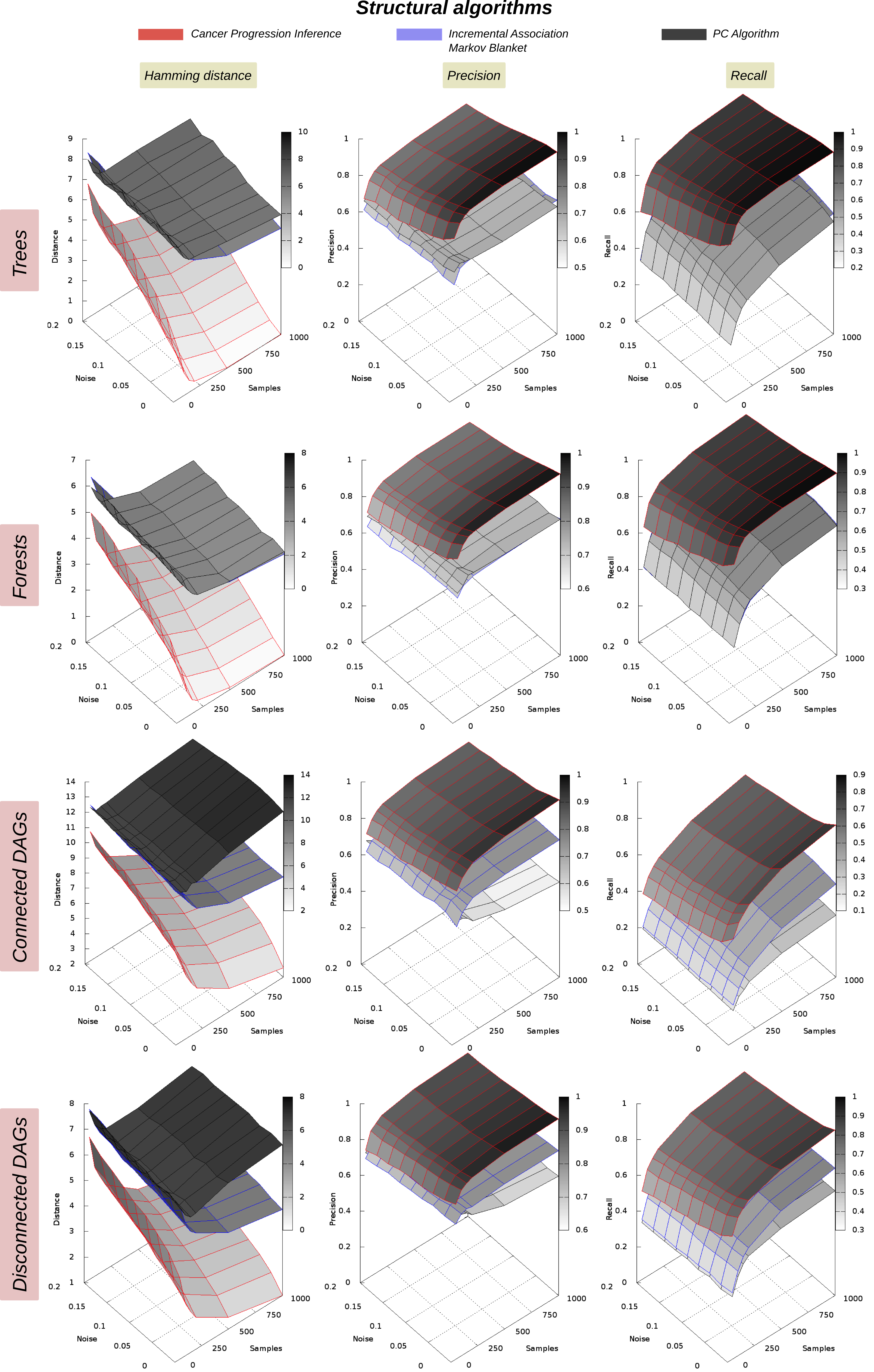
The general trend is summarized in Figure 8, where we rank all of these algorithms according to their median performance, estimated as a function of noise and sample size, and provide the parameters used for comparison. In Figure 9, we compare CAPRI with the structural approaches (IAMB and PC). In Figure 10, we compare it with the likelihood approaches (BIC and BDE) and, finally, in Figure 11, we compare it with the hybrid algorithms. We remark that, because of the high computational cost of running CBNs, which relies on a nested Expectation-Maximization algorithm with Simulated Annealing, the number of ensembles performed is limited to for CBNs, while it is for all other algorithms. Though this strategy provides less robust statistics for CBNs (i.e., less “smooth” performance surfaces), it is still sufficiently accurate to indicate the general comparative trends and relative performance efficiency.
C.3 Reconstruction without hypotheses: disjunctive patterns
Recall that our algorithm expects as input all the hypothesized patterns to infer more expressive logical formulas, i.e., hypotheses with pure CNF formulas or even disjunctive patterns over atomic events. Nonetheless, it is instructive to investigate its performance under two specific conditions, especially to clarify the robustness with respect to imperfect regularities (the, e.g, “noisy and”): namely, without hypotheses () and for datasets sampled from topologies with disjunctive patterns.
To generate the input dataset, we have to modify the generative procedure used for the other tests, thus reflecting the switch from co-occurrence to disjunctive patterns. This task is actually rather simple, since we just change the labeling function to account for the probability of picking any subset of the clauses in the disjunctive pattern, while omitting the others. We use DAGs with events and disjunctive patterns with at most atomic events involved, which is a reasonable size, given the events considered. Clearly, this setting is generally harder than the one shown in Figures 9– 11, thus we expect performance to be somewhat inferior. Here we compare CAPRI with all the algorithms used so far, and we show the result of this comparison in Figure 12, where , as noted earlier. The plot clearly confirms the trends suggested by previous analyses: namely, CAPRI infers the correct patterns more often than the others. Note also that the performance is measured on the reconstructed topology only, since, without input hypotheses, the algorithm evaluates only co-occurrence types of patterns, and does not allow different types of relations (e.g. disjunctions) to be inferred automatically. However, as anticipated, observed performance improvement is now much lower, and the Hamming distance fails to rise above . Furthermore, convergence to optimal performance was not observed for , and it appears not to be reachable even for (at least so, when no hypotheses are used). It is also possible that, as and the number of maximum disjunctive patterns increase, the result could be an even less satisfactory speed of convergence.
C.4 Reconstruction with hypotheses: synthetic lethality
We wondered whether CAPRI would be able to infer synthetic lethality relations, when these are directly hypothesized in the input set . We started with a test of the simplest form: e.g., for a set of events , where we force progression from to to be preferential, i.e. it appears with probability, whereas to does so with only probability, thus implying that samples involving will be more abundant than those involving . Despite this being the smallest possible synthetically lethal pattern, the goal was to estimate the probability of such a pattern being robustly inferable, when , and its dependence on the sample size and noise. We measured the performance of all the algorithms, with an input lifted according to the pattern so that all algorithms start with the same initial pieces of information. The performance metric estimates how likely an edge from to could be found in the reconstructed structures.
We show the results of this comparison in Figure 13. We note that CAPRI succeeds in inferring the synthetic lethality relation more frequently than of the times, irrespective of the noise and sample size used. More precisely, with the algorithm infers the correct pattern under any execution, thus suggesting that CAPRI, with the correct input hypotheses, is able to infer complicated structures, many of which could have high biological significance. Naturally, it would be reasonably expected that the performance of any of these algorithms would drop, were the target relations part of a bigger model.
C.5 Execution time
We report an evaluation of the execution time for all the algorithms we tested, but CBN - which computation time is more than one order of magnitude higher than the competing techniques. Two distinct settings of experiments were used: Setting : events, samples, noise; Setting : , , . Results account for the average time of execution as of randomly generated topologies (one dataset sampled per topology). Time unit is second and the test was performed on a MacBook with GHz Intel i7 processor, Gb of RAM and Yosemite 10.9 OS.
To allow a fair comparison of CAPRI against the other algorithms we both executed the algorithm with and without bootstrap preprocessing, in order to asses the prima facie condition (Mann-Withney U test being performed in the former case). Execution timings are sorted according to mean time.
| Setting A () | mean | median | standard deviation |
|---|---|---|---|
| CAPRESE | |||
| BIC | |||
| IAMB | |||
| CAPRI without bootstrap | |||
| BDE | |||
| PC | |||
| CAPRI with bootstrap |
| Setting B () | mean | median | standard deviation |
|---|---|---|---|
| CAPRESE | |||
| BIC | |||
| IAMB | |||
| CAPRI without bootstrap | |||
| BDE | |||
| PC | |||
| CAPRI with bootstrap |
Appendix D Biological examples
D.1 Atypical Chronic Myeloid Leukemia
Input hypotheses for CAPRI (supervised mode)
By fetching the literature we selected the following patterns to input as CAPRI’s hypotheses:
-
“exclusivity among asxl1 and sf3b1 mutations” [36]:
(asxl1 Nonsense point asxl1 Ins/del ) sf3b1 Missense point
-
“exclusivity among tet2 and idh2 mutations” [37]:
(tet2 Nonsense point tet2 Missense point tet2 Ins/del ) idh2 Missense point
These patterns were used to build CAPRI’s hypotheses which were tested against all events which do not appear in the above pattern itself, e.g., pattern (1) was tested against all input events but those involving asxl1 and sf3b1 genes.
As shown in the main text, among all, the following hypothesis gets selected by CAPRI
(asxl1 Nonsense point asxl1 Ins/del ) sf3b1 Missense point cbl Missense point
aCML progression model with different techniques
In Figure 14 one can find the progression models reconstructed on the the aCML dataset [16], with 3 different algorithms: CAPRESE, BIC and IAMB. These three techniques were chosen for this comparative study because of the overall better performance on synthetic tests (see Section 3.2-3.4 of the SI). The reconstruction obtained with CAPRI can be found in Figure 5 in the main text. For a biological interpretation of the results please refer to Section 4.2 in the main text.
Note that all the progression model share some specific selective advantage relations, yet being substantially different. Relations involving setbp1 and asxl1 and those involving tet2 and ezh2 are, in fact, inferred by all the four algorithms, yet with different confidences and, sometimes, edge direction. In addition, IAMB does not include cbl in the path involving setbp1 and asxl1, and none of the algorithms but CAPRI can infer the complex pattern involving asxl1 mutations of both types and sf3b1 (Figure 5 in the main text). Finally, note that IAMB and BIC are often not able to disambiguate the edge direction and this represent a major limit of these techniques with respect to CAPRI and CAPRESE.
D.2 Ovarian cancer
Ovarian cancer progression model with different techniques
We analyzed an ovarian cancer dataset reporting chromosome-level amplifications and deletions detected via Comparative Genome Hybridization in [48]. Similar to the case of aCML, we used 4 different techniques to infer a progression models for events included in the dataset: CAPRI (unsupervised), CAPRESE, BIC and IAMB. Models and input dataset are shown in Figure 15. Like with aCML extraction, the progression models share only some of the inferred relations. Among the most relevant differences is the conjunctive pattern inferred by CAPRI between the loss on chromosome 5q () and the gain on chromosome 8q () which is predicted to select for a loss on ; note also the aforementioned limitation of BIC and IAMB in disambiguating the direction of some of the inferred relations. Note that CAPRI infers a co-occurrence pattern of selective advantage which is not input a priori as hypothesis - unsupervised execution. In summary, CAPRI displays a better overall confidence on the reconstructed model.


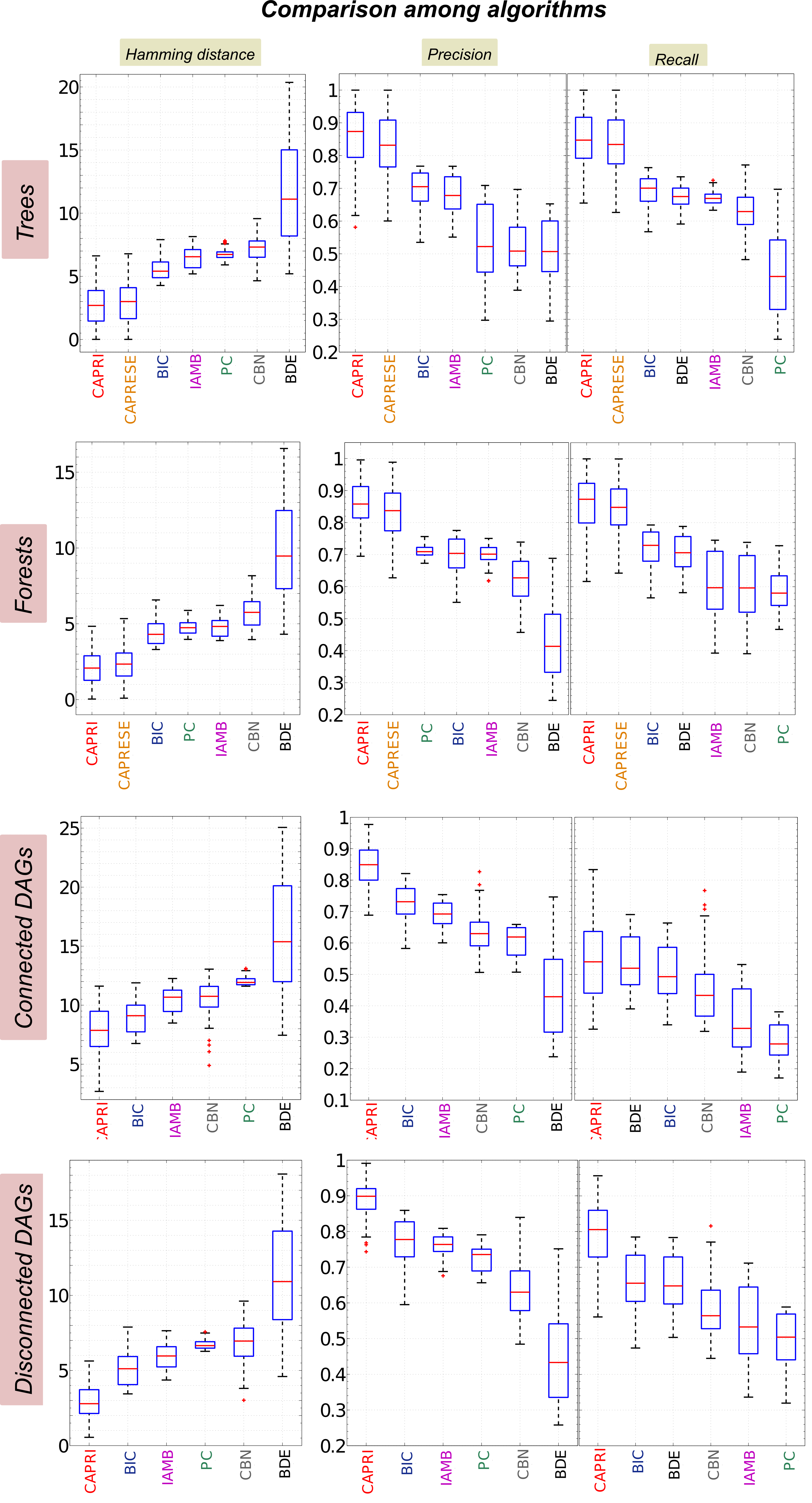
| Parameter values | ||
|---|---|---|
| number of events | ||
| number of samples | ||
| rate of false positives and negatives | (- noise rate) | |
| ensemble size | ( for CBN) | |