High-precision quark masses and QCD coupling
from $n_{f}=4$ lattice QCD

Bipasha Chakraborty Affiliation: SUPA, School of Physics and Astronomy, University of Glasgow, Glasgow, G12 8QQ, UK C. T. H. Davies Affiliation: SUPA, School of Physics and Astronomy, University of Glasgow, Glasgow, G12 8QQ, UK G. C. Donald Affiliation: Institut für Theoretische Physik, Universität Regensburg, 93040 Regensburg, Germany R. J. Dowdall Affiliation: DAMTP, University of Cambridge, Wilberforce Road, Cambridge, CB3 0WA, UK B. Galloway Affiliation: SUPA, School of Physics and Astronomy, University of Glasgow, Glasgow, G12 8QQ, UK P. Knecht Affiliation: SUPA, School of Physics and Astronomy, University of Glasgow, Glasgow, G12 8QQ, UK J. Koponen Affiliation: SUPA, School of Physics and Astronomy, University of Glasgow, Glasgow, G12 8QQ, UK G. P. Lepage Email: g.p.lepage@cornell.edu Affiliation: Laboratory for Elementary-Particle Physics, Cornell University, Ithaca, NY 14853, USA C. McNeile Affiliation: School of Computing and Mathematics and Centre for Mathematical Science, Plymouth University, Plymouth PL4 8AA, United Kingdom HPQCD Collaboration Affiliation:

4 December 2014

Abstract

We present a new lattice QCD analysis of heavy-quark pseudoscalar-pseudoscalar correlators, using gluon configurations from the MILC collaboration that include vacuum polarization from $u$ , $d$ , $s$ and $c$ quarks ( $n_{f}=4$ ). We extract new values for the QCD coupling and for the $c$ quark’s $\mathrm{\overline{MS}}$ mass: $\alpha_{\mathrm{\overline{MS}}}(M_{Z},n_{f}=5)=0.11822(74)$ and $m_{c}(3\,\mathrm{GeV},n_{f}=4)=0.9851(63)$ GeV. These agree well with our earlier simulations using $n_{f}=3$ sea quarks, vindicating the perturbative treatment of $c$ quarks in that analysis. We also obtain a new nonperturbative result for the ratio of $c$ and $s$ quark masses: $m_{c}/m_{s}=11.652(65)$ . This ratio implies $m_{s}(2\,\mathrm{GeV},n_{f}=3)=93.6(8)$ MeV when it is combined with our new $c$ mass. Combining $m_{c}/m_{s}$ with our earlier $m_{b}/m_{c}$ gives $m_{b}/m_{s}=52.55(55)$ , which is several standard deviations (but only 4%) away from the Georgi-Jarlskop prediction from certain GUTs. Finally we obtain an $n_{f}=4$ estimate for $m_{b}/m_{c}=4.528(54)$ which agrees well with our earlier $n_{f}=3$ result. The new ratio implies $m_{b}(m_{b},n_{f}=5)=4.162(48)$ GeV.

pacs

11.15.Ha,12.38.Aw,12.38.Gc

I Introduction

The precision of lattice QCD simulations has increased dramatically over the past decade, with many calculations now delivering results with 1–2% errors or less. Such precision requires increasingly accurate values for the fundamental QCD parameters: the quark masses and the QCD coupling. Accurate QCD parameters are important for non-QCD phenomenology as well. For example, theoretical uncertainties in several of the most important Higgs branching fractions are currently dominated by uncertainties in the heavy-quark masses (especially $m_{b}$ and $m_{c}$ ) and the QCD coupling [*[Forareviewsee][]Lepage:2014fla].

In this paper we present new lattice results for $m_{c}$ , $m_{c}/m_{s}$ , $m_{s}$ , $m_{b}/m_{c}$ , $m_{b}$ , and $\alpha_{s}$ . In a previous paper [2] we obtained 0.6%-accurate results for the masses and coupling by comparing continuum perturbation theory with nonperturbative lattice-QCD evaluations of current-current correlators for heavy-quark currents. Current-current correlators are particularly well suited to a perturbative analysis because non-perturbative effects are suppressed by four powers of $\Lambda_{\mathrm{QCD}}/2m_{h}$ where $m_{h}$ is the heavy-quark mass. Our earlier simulations treated $u$ , $d$ and $s$ sea quarks nonperturbatively ( $n_{f}=3$ ), while assuming that contributions from $c$ and heavier quarks can be computed using perturbation theory. Here we test the assumption that heavy-quark contributions are perturbative by repeating our analysis with lattice simulations that treat the $c$ quark nonperturbatively ( $n_{f}=4$ in the simulation).

In Section 2 we present our new $n_{f}=4$ lattice-QCD analysis of current-current correlators, leading to new results for the heavy-quark masses and the QCD coupling. We introduce an improved procedure that gives smaller errors and simplifies the analysis. We also demonstrate how our Monte Carlo data correctly reproduce the running of the $\mathrm{\overline{MS}}$ masses and coupling. In Section 3, we use the same simulations to calculate a new nonperturbative result for the ratio of the $c$ to $s$ quark masses, $m_{c}/m_{s}$ . In Section 4, we use these simulations to calculate the mass ratio $m_{h}/m_{c}$ for heavy quarks with masses $m_{h}$ between $m_{c}$ and $m_{b}$ . We express the ratio as a function of the heavy quark’s pseudoscalar mass $m_{\eta_{h}}$ . We extrapolate our result to $m_{\eta_{h}}=m_{\eta_{b}}$ to obtain a new nonperturbative estimate for $m_{b}/m_{c}$ . In Section 5, we summarize our conclusions, derive new values for the $s$ and $b$ masses, and present our thoughts about further work in this area. We also include, in Appendix A, a detailed discussion about how the coupling constant, quark masses, and the lattice spacing depend upon sea-quark masses in our approach. Our current analysis includes $u/d$ sea-quark masses down to physical values, so we are able to analyze this in far more detail than before. Finally, Appendix B briefly summarizes $n_{f}=4$ results obtained using our previous methods [2].

II Lattice Results

Our new analysis follows our earlier work [2], but with a simpler and more accurate method for connecting current correlators to $\mathrm{\overline{MS}}$ masses. In particular, this method allows us to determine the $\mathrm{\overline{MS}}$ $c$ mass at multiple scales, from correlators with different heavy-quark masses, providing a new test of our use of continuum perturbation theory. While the lattice spacings are not as small as before, our new analysis treats $c$ -quarks in the quark sea nonperturbatively. We also use the substantially more accurate HISQ discretization for the sea-quark action [3], in place of the ASQTAD discretization in our earlier analysis, and a more accurate method for setting the lattice spacing. The gluon action is also improved over our earlier analysis, as it now includes ${\cal O}(n_{f}\alpha_{s}a^{2})$ corrections [4]. Our new results also have more statistics, and include ensembles with $u/d$ masses very close to the physical value.

II.1 Heavy-Quark Correlator Moments

As before, we compute (temporal) moments

G_{n}\equiv\sum_{t}(t/a)^{n}G(t)

(1)

of correlators formed from the pseudoscalar density operator of a heavy quark, $j_{5}\equiv\overline{\psi}_{h}\gamma_{5}\psi_{h}$ :

G(t)=a^{6}\sum_{\mathbf{x}}(am_{0h})^{2}\langle 0|j_{5}(\mathbf{x},t)j_{5}(0,0)|0\rangle.

(2)

Here $m_{0h}$ is the heavy quark’s bare mass (from the lattice QCD lagrangian), $a$ is the lattice spacing, time $t$ is Euclidean and periodic with period $T$ , and the sum over spatial positions $\mathbf{x}$ sets the total three-momentum to zero. We again reduce finite-lattice spacing, tuning and perturbative errors by replacing the moments in our analysis with reduced moments:

\tilde{R}_{n}\equiv\left\{\begin{aligned} &G_{4}/G^{(0)}_{4}&&\text{for $n=4$,}\\ &\frac{1}{m_{0c}}\left(G_{n}/G^{(0)}_{n}\right)^{1/(n-4)}&&\text{for $n\geq 6$,}\end{aligned}\right.

(3)

where $G^{(0)}_{n}$ is the moment in lowest-order weak-coupling perturbation theory using the lattice regulator, and $m_{0c}$ is the bare mass of the $c$ quark.

Low- $n$ moments are dominated by short-distance physics because the correlator is evaluated at zero total energy, which is well below the threshold for on-shell hadronic states: the threshold is at $E_{\mathrm{threshold}}=m_{\eta_{h}}$ where

\mbox{2.9\,GeV}\leq m_{\eta_{h}}<\mbox{6.6\,GeV}

(4)

for our range of masses $m_{0h}$ . Furthermore, the moments are independent of the ultraviolet cutoff when $n\geq 4$ . Applying the Operator Product Expansion (OPE) to the product of currents in the correlator, we can therefore write our $n=4$ reduced moment in terms of continuum quantities,

$\displaystyle\tilde{R}_{4}\to\,$	$\displaystyle r_{4}(\alpha_{\mathrm{\overline{MS}}},\mu)\left\{1+\vphantom{\sum_{q=u,d,s}\frac{\langle m_{q}\overline{\psi}_{q}\psi_{q}\rangle}{(2m_{h})^{4}}}\right.$
	$\displaystyle+d_{4}^{\mathrm{cond}}(\alpha_{\mathrm{\overline{MS}}},\mu)\frac{\langle\alpha_{s}G^{2}/\pi\rangle_{\mathrm{eff}}}{(2m_{h})^{4}}$
	$\displaystyle\left.+\tilde{d}_{4}^{\mathrm{cond}}(\alpha_{\mathrm{\overline{MS}}},\mu)\sum_{q=u,d,s}\frac{\langle m_{q}\overline{\psi}_{q}\psi_{q}\rangle_{\mathrm{eff}}}{(2m_{h})^{4}}+\cdots\right\},$	(5)

in the continuum limit ( $a\to 0$ ). Here $\alpha_{\overline{\mathrm{MS}}}$ is the $\mathrm{\overline{MS}}$ coupling at scale $\mu$ , and $m_{h}$ is the $\mathrm{\overline{MS}}$ $h$ -quark mass. Heavy-quark condensates are absorbed into the gluon condensate [5]. We will retain terms only through the gluon condensate in what follows since its contribution is already very small and contributions from other condensates will be much smaller. We discuss the precise meaning of $\langle\alpha_{s}G^{2}/\pi\rangle_{\mathrm{eff}}$ below. Reduced moments with $n\geq 6$ can be written:

	$\displaystyle\tilde{R}_{n}\to\,$	$\displaystyle\frac{r_{n}(\alpha_{\mathrm{\overline{MS}}},\mu)}{m_{c}(\mu)}\left\{1\vphantom{\frac{\langle\alpha_{s}G^{2}/\pi\rangle}{(2m_{h})^{4}}}\right.$
		$\displaystyle+\left.d_{n}^{\mathrm{cond}}(\alpha_{\mathrm{\overline{MS}}},\mu)\frac{\langle\alpha_{s}G^{2}/\pi\rangle_{\mathrm{eff}}}{(2m_{h})^{4}}+\cdots\right\},$		(6)

where $m_{c}(\mu)$ is the $\mathrm{\overline{MS}}$ mass of the $c$ quark. The continuum expressions for $\tilde{R}_{n}$ should agree with tuned lattice simulations up to finite-lattice-spacing errors of $\mathcal{O}((am_{h})^{2}\alpha_{s})$ . The perturbative expansions for the coefficient functions $r_{n}$ are known through third order: see Table 1 and [6, 7, 8, 9, 10]. The expansions for $d_{n}^{\mathrm{cond}}$ are known through first order [11].

Table 1: Perturbation theory coefficients for

r_{n}

with

n_{f}=4

sea quarks, where the heaviest sea quark has the same mass

m_{h}

as the valence quark (that is, the quark used to make the currents in the current-current correlator). Coefficients are defined by

r_{n}=1+\sum_{j}r_{nj}\alpha_{\mathrm{\overline{MS}}}^{j}(\mu)

where

\mu=m_{h}(\mu)

. These coefficients are derived in [6, 7, 8, 9, 10].

$n$	$r_{n1}$	$r_{n2}$	$r_{n3}$
4	$0.7427$	$0.0088$	$-0.0296$
6	$0.6160$	$0.4976$	$-0.0929$
8	$0.3164$	$0.3485$	$0.0233$
10	$0.1861$	$0.2681$	$0.0817$

Parameter $\mu$ sets the scale for $m_{c}$ and for $\alpha_{\mathrm{\overline{MS}}}$ in $r_{n}$ . As in our previous paper, we take

\mu=3m_{h}(\mu)

(7)

in order to improve the convergence of perturbation theory. In fact, however, our method is almost completely independent of the choice of $\mu$ , by design. We can reexpress $\mu$ in terms of the $\mathrm{\overline{MS}}$ mass of the $c$ quark,

\mu=3m_{c}(\mu)\frac{m_{0h}}{m_{0c}},

(8)

since ratios of quark masses are regulator independent: that is,

\frac{m_{0h}}{m_{0c}}=\frac{m_{h}(\mu)}{m_{c}(\mu)}

(9)

up to $a^{2}$ errors (for any $\mu$ ).

Our reduced moments differ for $n\geq 6$ from our earlier work: here we multiply by $1/m_{0c}$ in Eq. (3) instead of $m_{\eta_{h}}/2m_{0h}$ . The ratio of $G$ s in $\tilde{R}_{n\geq 6}$ introduces a factor of $m_{0h}/m_{h}(\mu)$ . This becomes $1/m_{c}(\mu)$ when multiplied by $1/m_{0c}$ (by Eq. (9)). Consequently we can use moments calculated with any heavy-quark mass $m_{0h}$ to estimate the $\mathrm{\overline{MS}}$ $c$ mass (at $\mu=3m_{h}(\mu)$ ). Consistency among $m_{c}$ s coming from different $m_{0h}$ values is an important test of the formalism.

We could have used the bare mass of any quark, in place of $m_{0c}$ , in Eq. (3). Then the $n\geq 6$ moments would give values for the $\mathrm{\overline{MS}}$ mass of that quark. Alternatively we could leave the quark mass factor out, in which case these moments give the factors $Z_{m}(\mu)$ that convert any bare lattice quark mass into the corresponding $\mathrm{\overline{MS}}$ mass at scale $\mu$ . Heavy-quark current-current correlators, as used here, provide an alternative to RI-mom [12] and similar methods for determining both light and heavy quark masses.

The new definition for the reduced moments simplifies our analysis since the variation of factor $m_{c}(\mu)$ with $\mu$ is well known from perturbative QCD. The $m_{\eta_{h}}$ dependence of the analogous factor ( $m_{\eta_{h}}/2m_{h}$ ) in the old analysis is unknown a priori, and so must be modeled in the fit. We analyzed our data using the old definitions; the results, which agree with the results we find with the new methods, are described briefly in Appendix B.

II.2 Lattice Simulations

Table 2: Simulation parameters for the gluon ensembles used in this paper [13, 14], with lattice spacings of approximately 0.15, 0.12, 0.09 and 0.06 fm, and various combinations of sea-quark masses. The parameters for each simulation are: the inverse lattice spacing in units of

w_{0}=0.1715(9)

fm, the spatial

L

and temporal

T

lattice lengths, the number of gluon configurations

N_{\mathrm{cf}}

(each with multiple time sources), the bare sea-quark masses in lattice units (

am_{0\ell},am_{0s},am_{0c}

), and the tuned bare

s

and

c

quark masses in GeV. The tuned

s

and

c

masses gives physical values for the

\eta_{s}

and

\eta_{c}

mesons, respectively. The

\ell

mass is the average of the

u

and

d

masses, which are set equal in our simulations.

Z_{m}(\mu)

is the ratio of the

\mathrm{\overline{MS}}

quark mass

m_{q}(\mu,n_{f}=4)

to the corresponding bare (lattice) mass

m_{0q}

(see Section II.4). The last two entries for each ensemble indicate the degree to which the sea-quark masses are detuned (see Appendix A).

ensemble	$\quad w_{0}/a$	$L/a$	$T/a$	$N_{\mathrm{cf}}$	$am_{0\ell}$	$am_{0s}$	$am_{0c}$	$m_{0s}^{\mathrm{tuned}}$	$m_{0c}^{\mathrm{tuned}}$	$Z_{m}(3\,\mathrm{GeV})$	$\delta m_{uds}^{\mathrm{sea}}/m_{s}$	$\delta m_{c}^{\mathrm{sea}}/m_{c}$
1	1.1119(10)	16	48	1020	0.01300	0.0650	0.838	0.0895(7)	1.138(4)	0.866(5)	0.228(16)	$-0$ .058(8)
2	1.1272(7)	24	48	1000	0.00640	0.0640	0.828	0.0890(7)	1.130(4)	0.872(6)	0.046(14)	$-0$ .050(8)
3	1.1367(5)	36	48	1000	0.00235	0.0647	0.831	0.0885(7)	1.125(4)	0.876(5)	$-0$ .048(13)	$-0$ .034(8)
4	1.3826(11)	24	64	300	0.01020	0.0509	0.635	0.0866(7)	1.057(3)	0.933(6)	0.236(16)	$-0$ .044(8)
5	1.4029(9)	32	64	300	0.00507	0.0507	0.628	0.0861(7)	1.051(3)	0.938(6)	0.067(14)	$-0$ .035(8)
6	1.4149(6)	48	64	200	0.00184	0.0507	0.628	0.0857(7)	1.047(3)	0.941(6)	$-0$ .040(13)	$-0$ .024(8)
7	1.9330(20)	48	96	300	0.00363	0.0363	0.430	0.0823(9)	0.977(3)	1.009(6)	0.104(11)	$-0$ .021(8)
8	1.9518(7)	64	96	304	0.00120	0.0363	0.432	0.0818(7)	0.973(3)	1.013(6)	$-0$ .011(13)	$-0$ .003(8)
9	2.8960(60)	48	144	333	0.00480	0.0240	0.286	0.0778(7)	0.912(3)	1.080(7)	0.365(19)	0.045(9)

To extract the coupling constant and $c$ mass from simulations, we use the simulations to compute nonperturbative values for the reduced moments $\tilde{R}_{n}$ with small $n\geq 4$ and a range of heavy-quark masses $m_{0h}$ . We vary the lattice spacing, so we can extrapolate to zero lattice spacing, and the sea-quark masses, so we can tune the masses to their physical values.

The gluon-field ensembles we use come from the MILC collaboration and include $u$ , $d$ , $s$ , and $c$ quarks in the quark sea [13, 14]. The parameters that characterize these ensembles are given in Table 2. The highly accurate HISQ discretization [3] is used here for both the sea quarks and the heavy quarks in the currents used to create the correlators. This discretization was designed to minimize $(am_{h})^{2}$ errors for large $m_{h}$ . Our previous work used HISQ quarks in the currents, but a less accurate discretization (ASQTAD) for the sea quarks.

We also quote tuned values for the bare $s$ and $c$ quark masses in Table 2. These are the quark masses that give the physical values for the $\eta_{s}$ and $\eta_{c}$ masses, as discussed in Appendix A.1. This is the bare $c$ mass we use in Eq. (3) for $\tilde{R}_{n}$ .

Table 3: Simulations results for

\eta_{h}

masses and reduced moments with various bare heavy-quark masses

am_{0h}

and gluon ensembles (first column, see Table 2). Only data for

am_{0h}\leq 0.8

are used in fits to the correlators.

	$am_{0h}$	$\quad am_{\eta_{h}}$	$\tilde{R}_{4}$	$\tilde{R}_{6}$	$\tilde{R}_{8}$	$\tilde{R}_{10}$
1	0.826	2.22510(10)	1.1627(1)	0.937(3)	0.885(3)	0.856(3)
	0.888	2.33188(9)	1.1477(1)	0.937(3)	0.893(3)	0.867(3)
2	0.818	2.21032(6)	1.1643(0)	0.943(3)	0.890(3)	0.860(3)
3	0.863	2.28770(4)	1.1528(0)	0.947(3)	0.900(3)	0.872(3)
4	0.645	1.83976(11)	1.1842(2)	0.986(3)	0.915(3)	0.874(2)
	0.663	1.87456(12)	1.1783(2)	0.988(3)	0.919(3)	0.880(2)
5	0.627	1.80318(8)	1.1896(1)	0.989(3)	0.915(3)	0.874(2)
	0.650	1.84797(8)	1.1819(1)	0.992(3)	0.921(3)	0.881(2)
	0.800	2.13055(7)	1.1409(1)	1.001(3)	0.951(3)	0.920(3)
6	0.637	1.82225(5)	1.1860(1)	0.994(3)	0.921(3)	0.880(2)
7	0.439	1.34246(4)	1.2134(1)	1.013(3)	0.921(3)	0.877(2)
	0.500	1.47051(4)	1.1886(1)	1.029(3)	0.946(3)	0.903(3)
	0.600	1.67455(4)	1.1565(1)	1.048(3)	0.978(3)	0.939(3)
	0.700	1.87210(4)	1.1315(0)	1.059(3)	1.002(3)	0.968(3)
	0.800	2.06328(3)	1.1118(0)	1.064(3)	1.019(3)	0.991(3)
8	0.433	1.32929(3)	1.2160(1)	1.015(3)	0.922(3)	0.877(2)
	0.500	1.47012(3)	1.1885(0)	1.033(3)	0.950(3)	0.906(2)
	0.600	1.67418(3)	1.1564(0)	1.052(3)	0.982(3)	0.943(3)
	0.700	1.87177(2)	1.1315(0)	1.063(3)	1.006(3)	0.972(3)
	0.800	2.06297(2)	1.1117(0)	1.068(3)	1.023(3)	0.995(3)
9	0.269	0.88525(5)	1.2401(4)	1.011(3)	0.913(3)	0.869(2)
	0.274	0.89669(5)	1.2368(4)	1.014(3)	0.917(3)	0.873(2)
	0.400	1.17560(5)	1.1752(2)	1.068(3)	0.985(3)	0.944(3)
	0.500	1.38750(4)	1.1440(2)	1.094(3)	1.023(3)	0.985(3)
	0.600	1.59311(4)	1.1204(1)	1.112(3)	1.051(3)	1.017(3)
	0.700	1.79313(4)	1.1018(1)	1.122(3)	1.073(3)	1.043(3)
	0.800	1.98751(3)	1.0867(1)	1.127(3)	1.088(3)	1.063(3)
	0.900	2.17582(3)	1.0823(0)	1.399(4)	1.246(3)	1.169(3)
	1.000	2.35773(3)	1.0284(0)	1.442(4)	1.295(4)	1.215(3)

In Table 3 we list our simulation results for the $\eta_{h}$ mass and the reduced moments for various bare quark masses $am_{0h}$ on various ensembles. Results from different values of $am_{0h}$ on the same ensemble are correlated; we include these correlations in our analysis. The $am_{\eta_{h}}$ values are computed from Bayesian fits of multi-state function

\sum_{j=1}^{10}b_{j}\left(e^{-m_{j}t}+e^{-m_{j}(T-t)}\right)

(10)

to the correlators $G(t)$ for $t\geq 8$ , where $T$ is the temporal length of the lattice [15]. The fitting errors are small for $am_{\eta_{h}}$ and have minimal impact on our final results.

The fractional errors in the $\tilde{R}_{n}$ for $n\geq 6$ are 20–40 times larger than those for $\tilde{R}_{4}$ . This is because of the factor of $1/m_{0c}^{\mathrm{tuned}}$ used in Eq. (3) to define these moments. As mentioned above, we could have used bare masses for other quarks in this definition, to obtain values for their $\mathrm{\overline{MS}}$ masses. Heavy-quark masses like $m_{0c}$ , however, can usually be tuned more accurately than light-quark masses, as discussed in Appendix A. Masses for other quarks can be obtained from the $c$ mass and nonperturbatively determined quark mass ratios, as we show for the $s$ and $b$ masses in the next two sections.

As in our previous paper, we limit the maximum size of $am_{h}$ in our analysis: we require $am_{h}\leq 0.8$ . This keeps $a^{2}$ errors smaller than 10%.

We determine the lattice spacing by measuring the Wilson flow parameter $w_{0}/a$ on the lattice (Table 2) [16]. From previous simulations [17], we know that

w_{0}=0.1715(9)\,\mathrm{fm},

(11)

which we combine with our measured values of $w_{0}/a$ to obtain the lattice spacing for each ensemble (Appendix A). This approach is far more accurate than that used in our earlier paper, which relied upon the $r_{1}$ parameter from the static-quark potential.

II.3 Fitting Lattice Data

Our goal is to find values for $\alpha_{\mathrm{\overline{MS}}}(\mu)$ and $m_{c}(\mu)$ that make the theoretical results (from perturbation theory) for the reduced moments $\tilde{R}_{n}$ (Eqs. (5–6)) agree with the nonperturbative results from our simulations. We do this by simultaneously fitting results from all of our lattice spacings and quark masses for moments with $4\leq n\leq 10$ . To get good fits, we must correct the continuum formulas in Eqs. (5–6) for several systematic errors in the simulation. We fit the lattice data using the following corrected form:

$\displaystyle\tilde{R}_{n}$	$\displaystyle=\left.\begin{cases}1&\mbox{for $n=4$}\\ 1/\xi_{m}m_{c}(\xi_{\alpha}\mu)&\mbox{for $n\geq 6$}\end{cases}\right\}$	(12)
	$\displaystyle\times r_{n}(\alpha_{\mathrm{\overline{MS}}}(\xi_{\alpha}\mu),\mu)$	(13)
	$\displaystyle\times\left(1+d_{n}^{\mathrm{cond}}\frac{\langle\alpha_{s}G^{2}/\pi\rangle}{(2m_{h})^{4}}\right)$	(14)
	$\displaystyle\times\left(1+d_{n}^{h,c}\frac{m_{0h}^{2}-m_{0c}^{2}}{m_{0h}^{2}}\right)$	(15)
	$\displaystyle+\left(\frac{am_{\eta_{h}}}{2.26}\right)^{2}\sum_{i=0}^{N}c_{i}(m_{\eta_{h}},n)\left(\frac{am_{\eta_{h}}}{2.26}\right)^{2i}.$	(16)

We use a Bayesian fit with priors for every fit parameter [15]. The priors are a priori estimates for the parameters based upon theoretical expectations and previous experience, especially from our earlier, very similar $n_{f}=3$ analysis. In each case we test our choice of prior width against the Empirical Bayes criterion [15], which in effect uses fluctuations in the data to suggest natural widths for priors. None of our priors is narrower than this optimal width, and most are wider, which leads to more conservative errors.

We now explain each part of the lattice formula in turn.

II.3.1 Detuned Sea-quark Masses

The terms $\alpha_{\mathrm{\overline{MS}}}(\xi_{\alpha}\mu)$ and $\xi_{m}m_{h}(\xi_{\alpha}\mu)$ in $\tilde{R}_{n}$ are the $\mathrm{\overline{MS}}$ coupling and heavy-quark mass for detuned sea-quark masses; see Eqs. (68) and (78) in Appendix A. Scale $\mu$ is chosen so that

\mu=3\,\xi_{m}m_{c}(\xi_{\alpha}\mu)\frac{m_{0h}}{m_{0c}}=3\,m_{h}(\mu,\delta m^{\mathrm{sea}}).

(17)

Scale factors $\xi_{\alpha}$ and $\xi_{m}$ are defined in Appendix A, which discusses how $\mathrm{\overline{MS}}$ couplings and masses are affected by sea-quark masses. The coefficients $g_{\alpha}$ , $g_{m}$ …in $\xi_{\alpha}$ and $\xi_{m}$ are treated as fit parameters, with priors taken from the output of the fits described in the appendix.

The light sea-quark masses enter linearly in $\xi_{\alpha}$ and $\xi_{m}$ , because of (nonperturbative) chiral symmetry breaking. Quark mass dependence also enters through the perturbation theory for the moments ( $r_{n}$ ), but is quadratic in the mass and therefore negligible for light quarks.

II.3.2 $\mu$ Dependence

The scale $\mu$ enters Eqs. (12)–(16) through the coupling constant $\alpha_{\mathrm{\overline{MS}}}(\xi_{\alpha}\mu)$ and the $c$ mass $m_{c}(\xi_{\alpha}\mu)$ . We parameterize the coupling and mass in the fit by specifying their values at $\mu=5$ GeV with fit parameters $\alpha_{0}$ and $m_{0}$ ,

	$\displaystyle\alpha_{\mathrm{\overline{MS}}}(5\,\mathrm{GeV},n_{f}=4)=\alpha_{0}$
	$\displaystyle m_{c}(5\,\mathrm{GeV},n_{f}=4)=m_{0},$		(18)

whose priors are

\displaystyle\alpha_{0}=0.21\pm 0.02,\quad m_{0}=0.90\pm 0.10.

(19)

Our previous analysis gave $0.2134(24)$ and $0.8911(56)$ for these parameters, so the priors are broad. The coupling and mass for other values of $\mu$ are obtained by integrating (numerically) their evolution equations from perturbative QCD, starting from the values at $\mu=5$ GeV:

$\displaystyle\mu^{2}\frac{d\alpha_{\mathrm{\overline{MS}}}(\mu)}{d\mu^{2}}=$	$\displaystyle-\beta_{0}\alpha_{\mathrm{\overline{MS}}}^{2}(\mu)-\beta_{1}\alpha_{\mathrm{\overline{MS}}}^{3}-\beta_{2}\alpha_{\mathrm{\overline{MS}}}^{4}$
	$\displaystyle-\beta_{3}\alpha_{\mathrm{\overline{MS}}}^{5}-\beta_{4}\alpha_{\mathrm{\overline{MS}}}^{6},$	(20)
$\displaystyle\frac{d\log m_{h}(\mu)}{d\log\mu^{2}}=$	$\displaystyle-\gamma_{0}\alpha_{\mathrm{\overline{MS}}}(\mu)-\gamma_{1}\alpha_{\mathrm{\overline{MS}}}^{2}-\gamma_{2}\alpha_{\mathrm{\overline{MS}}}^{3}$
	$\displaystyle-\gamma_{3}\alpha_{\mathrm{\overline{MS}}}^{4}-\gamma_{4}\alpha_{\mathrm{\overline{MS}}}^{5}.$	(21)

The first four coefficients on the right-hand-sides of these equations are known from perturbation theory [18, 19, 20, 21]. In each case, we treat the fifth coefficient as a fit parameter whose prior’s width equals the root-mean-square average of the first four parameters:

\displaystyle\beta_{4}=0\pm\sigma_{\beta},\quad\gamma_{4}=0\pm\sigma_{\gamma}.

(22)

Neither $\beta_{4}$ nor $\gamma_{4}$ has signficant impact on our final results.

II.3.3 Truncated Perturbation Theory

The Wilson coefficient function $r_{n}$ (Eq. (13)) has a perturbative expansion of the form

r_{n}(\alpha_{\mathrm{\overline{MS}}},\mu)\equiv 1+\sum_{j=1}^{N_{\mathrm{pth}}}r_{nj}(\mu)\alpha_{\mathrm{\overline{MS}}}^{j}.

(23)

The perturbative coefficients $r_{nj}$ are known through third order, and are given for $\mu=m_{h}(\mu)$ in Table 1.

The lack of perturbative coefficients beyond third order is our largest single source of systematic error. Our data are sufficiently precise that higher-order terms are relevant. Furthermore the relative importance of the higher-order terms varies with quark mass, as $\alpha_{\mathrm{\overline{MS}}}$ varies with $\mu=3m_{h}$ . Therefore we include the higher-order terms in our analysis with coefficients that we fit to account for variations with quark mass. As in our earlier analysis, we note that the known perturbative coefficients are small and relatively uncorrelated from moment to moment and order to order for $\mu=m_{h}$ , leading us to adopt fit priors

r_{nj}(\mu=m_{h})=0\pm 1

(24)

for the $n>3$ coefficients at $\mu=m_{h}$ . We double the width of these priors relative to our previous analysis because the fit suggested that some higher-order coefficients are larger here (especially for $n=4$ ).

We set $N_{\mathrm{pth}}=15$ terms in the expansion, although our results are essentially unchanged once 8 or more terms are included (or 5 with $\mu=m_{h}$ ). As before we use renormalization group equations to express the coefficients $r_{nj}(\mu=3m_{h})$ in terms of the coefficients $r_{nj}(\mu=m_{h})$ from Table 1 and Eq. (24). This procedure generates (correlated) priors for the unknown coefficients at $\mu=3m_{h}$ that account for renormalization-group logarithms. The procedure makes our results largely independent of $\mu$ : our results change by less than a third of a standard deviation as $\mu$ is varied over the interval $2m_{h}\leq\mu\leq 10m_{h}$ .

II.3.4 Nonperturbative Effects; Finite-Volume Corrections

We use the Operator Product Expansion (OPE) in Eqs. (5–6) to separate short-distance from long-distance physics. In principle, the perturbative coefficients in $r_{n}(\alpha_{\mathrm{\overline{MS}}},\mu)$ above should have subtractions coming from the higher-order terms in the OPE expansion:

r_{n}\to r_{n}\left(1-d_{n}^{\mathrm{cond}}\frac{\langle\alpha_{s}G^{2}/\pi\rangle^{(\lambda)}_{\mathrm{pth}}}{(2m_{h})^{4}}-\cdots\right)

(25)

where $\lambda$ is a fixed cutoff scale in the perturbative regime, say $\lambda=1$ GeV, and $\langle\alpha_{s}G^{2}/\pi\rangle^{(\lambda)}_{\mathrm{pth}}$ and $d_{n}^{\mathrm{cond}}$ are computed in perturbation theory to the same order as $r_{n}$ . These subtractions come from perturbative matching, and remove contributions to $r_{n}$ due to low-momentum gluons ( $q\!\leq\!\lambda$ ), thereby also removing infrared renormalons order-by-order in perturbation theory. The size of the subtraction depends upon the detailed definition of $\alpha_{s}(G^{(\lambda)})^{2}$ . This procedure is completely unambiguous given a specific definition for this operator, but we have not included the subtraction in $r_{n}$ since it is negligible for any reasonable definition at our low orders of perturbation theory. For example, a simple momentum-space cutoff, that keeps $q^{2}<\lambda^{2}$ , gives [22]

\langle\alpha_{s}G^{2}\rangle^{(\lambda)}_{\mathrm{pth}}=\frac{3\alpha_{s}}{2\pi^{3}}\,\lambda^{4},

(26)

which ranges from 0.001 to 0.019 $\mathrm{GeV}^{4}$ for $\lambda$ s between 500 Mev and 1 GeV. This would change $r_{n}$ by no more than 0.1–0.4% at $m_{h}=m_{c}$ and much less at our higher $m_{h}$ s.

Not surprisingly, perturbative estimates of the condensate value (Eq. (26)) are similar in size to nonperturbative estimates of the condensate value. So it is simpler for us to combine the subtraction in Eq. (25) with the condensate itself to form an effective condensate value [23]:

\langle\alpha_{s}G^{2}\rangle_{\mathrm{eff}}\equiv\langle\alpha_{s}G^{2}\rangle^{(\lambda)}-\langle\alpha_{s}G^{2}\rangle^{(\lambda)}_{\mathrm{pth}}

(27)

In our fits we take $\langle\alpha_{s}G^{2}\rangle_{\mathrm{eff}}$ as a fit parameter with prior

\langle\alpha_{s}G^{2}\rangle_{\mathrm{eff}}=0.0\pm 0.012,

(28)

and we approximate $m_{h}\approx m_{\eta_{h}}/2.26$ in the condensate correction (because $m_{b}(m_{b})\approx m_{\eta_{b}}/2.26$ ). Our results are completely unchanged if the width of this prior is ten times larger. In either case we obtain a value for the effective condensate of order $0.002$ with errors of a similar size. This is completely consistent with expectations, and it reduces condensate contributions to the moments to 0.01–0.05% at $m_{h}=m_{c}$ , and much less at higher $m_{h}$ — negligible at our level of precision.

This procedure is sensible at our level of precision. As precision increases, however, there is a point where it becomes important to remove renormalon corrections from the coefficients in $r_{n}$ . Otherwise $j!$ factors in $j^{\mathrm{th}}$ order, coming from infrared renormalons, cause perturbation theory to diverge. A simple analysis [*[See, forexample, ][]Shifman:2013uka] indicates that perturbation theory starts to diverge at order $j\sim 2/(\beta_{0}\alpha_{\mathrm{\overline{MS}}})$ , which is around $8^{\mathrm{th}}$ order for our analysis. Consequently we expect the impact of infrared renormalons to be negligible at $3^{\mathrm{rd}}$ order.

Perturbation theory is not the whole story even if infrared renormalons are removed. The OPE separates short-distances from long-distances, but the short-distance coefficients $r_{n}$ , $d_{n}^{\mathrm{cond}}$ … have nonperturbative contributions, for example, from small instantons [22]. It is also possible that the OPE is an asymptotic expansion and does not converge ultimately, although recent results suggest it might converge [25, 26]. Whatever the case, such effects are expected to appear at even higher orders than infrared renormalons, and so are completely negligible at our level of precision.

Condensates, renormalons, small instantons, etc. afflict all perturbative analyses at some level of precision. Our analysis is particularly insensitive to such effects because the leading nonperturbative contributions are suppressed by four powers of $\Lambda_{\mathrm{QCD}}/(2m_{h})$ .

Note finally that the coefficient functions, being short-distance, are insensitive to errors caused by the finite volume of the lattice. While the finite volume can affect the value of $\langle\alpha_{s}G^{2}\rangle_{\mathrm{eff}}$ , the impact on our results is negligible since the condensate itself is negligible. We verified this by recalculating the reduced moments for emsemble 5 in Table 2 with spatial lattice sizes of $L/a=24$ and 40 (ensemble 5 uses 32). The moments for different volumes agree to within statistical errors of order 0.01%. The same is true for the measured values of $m_{\eta_{c}}$ from these ensembles; finite volume effects will be smaller still for $m_{\eta_{h}}$ .

II.3.5 $m_{0h}-m_{0c}$ Correction

Our results are also affected by the difference between the $c$ mass $m_{0c}$ used in the sea, and the mass of the heavy quark $m_{0h}$ used to make the currents in the current-current correlator. The perturbative calculations we use assume $m_{0c}=m_{0h}$ , but we want to study a range of $m_{0h}$ values with fixed $m_{0c}$ . The correction enters in ${\cal O}(\alpha_{s}^{2})$ , is quadratic in the mass difference for small differences, and goes to a (small) constant as $m_{0h}\to\infty$ . Therefore we correct for it using (Eq. (15))

\tilde{R}_{n}\to\tilde{R}_{n}\left(1+d_{n}^{h,c}\frac{m_{0h}^{2}-m_{0c}^{2}}{m_{0h}^{2}}\right)

(29)

where $h_{n}$ is a fit parameter with a prior of $0\pm 0.03$ . The width 0.03 is ten times larger than the correct value (from perturbation theory) in the $m_{0h}\to\infty$ limit. It is twice as wide as the width indicated by the Empirical Bayes criterion [15]. We also tried fits where $d_{n}^{h,c}$ was replaced by a spline function of $m_{\eta_{h}}$ . These give similar results but with larger errors (especially for $\alpha_{\mathrm{\overline{MS}}}$ ).

II.3.6 Finite Lattice Spacing Errors

The final modification in our formula for $\tilde{R}_{n}$ corrects for errors caused by the finite lattice spacings used in the simulations. We write

\tilde{R}_{n}\to\tilde{R}_{n}+\delta\tilde{R}_{n}

(30)

where

\delta\tilde{R}_{n}\equiv\left(\frac{am_{\eta_{h}}}{2.26}\right)^{2}\sum_{i=0}^{N}c_{i}^{(n)}(m_{\eta_{h}})\left(\frac{am_{\eta_{h}}}{2.26}\right)^{2i}

(31)

and again $m_{\eta_{h}}/2.26$ is a proxy for the quark mass. We parameterize the $m_{\eta_{h}}$ dependence of the $c_{i}^{(n)}(m_{\eta_{h}})$ using cubic splines with knots, at

m_{\mathrm{knots}}\equiv\mbox{\lx@text@lbrace 2.9, 3.6, 4.6, 7.9\lx@text@rbrace\,GeV},

(32)

that come from the analysis in Section IV. We set

c_{i}^{(n)}(m)=c_{0i}^{(n)}+\delta c_{i}^{(n)}(m)

(33)

with the following fit parameters and priors:

$\displaystyle c_{0i}^{(n)}$	$\displaystyle=0\pm 1/n$
$\displaystyle\delta c_{i}^{(n)}(m)$	$\displaystyle=0\pm 0.10/n$	$\displaystyle m\in m_{\mathrm{knots}}$
$\displaystyle\delta c_{i}^{(n)\prime}(m)$	$\displaystyle=0\pm 0.10/n$	$\displaystyle m=2.9\,\mathrm{GeV}.$	(34)

These priors are again conservative since the Empirical Bayes criterion [15] suggests priors that are half as wide. We take $N=20$ but our results are insensitive to any $N\geq 10$ .

II.4 $n_{f}=4$ Lattice Results

We fit all of the reduced moments from our simulation data — with lattice spacings from 0.12 fm to 0.06 fm, and $n=4$ , 6, 8 and 10 in Table 3 — simultaneously to formula (12–16) by adjusting fit parameters described in the previous sections. The fit is excellent with a $\chi^{2}$ per degree of freedom of 0.51 for 92 pieces of data ( $p$ -value is 1.0).

The fit has two key physics outputs. One is a new result for the running coupling constant:

\alpha_{\mathrm{\overline{MS}}}(5\,\mathrm{GeV},n_{f}=4)=0.2128(25).

(35)

To compare with our old determination and other determinations, we use perturbation theory to add $b$ quarks to the sea [27], with $m_{b}(m_{b})=4.164(23)$ GeV [2], and evolve to the $Z$ mass (91.19 GeV) to get

\alpha_{\mathrm{\overline{MS}}}(M_{Z},n_{f}=5)=0.11822(74).

(36)

This agrees well with $0.1183(7)$ from our $n_{f}=3$ analysis [2]. It also agrees well with the current world average 0.1185(6) from the Particle Data Group [*[][and2013partialupdateforthe2014edition.]Agashe:2014kda].

The second important physics output is the $c$ quark’s mass, whose value at $\mu=5$ GeV is a fit parameter:

m_{c}(\mu,n_{f}=4)=\begin{cases}0.8905(56)\,\mathrm{GeV}&\mu=5\,\mathrm{GeV}\\ 0.9851(63)\,\mathrm{GeV}&\mu=3\,\mathrm{GeV}\\ 1.2715(95)\,\mathrm{GeV}&\mu=m_{c}(\mu),\end{cases}

(37)

where we have used Eq. (21) to evolve our result to other scales for comparison with other determinations. These again agree well with our previous $n_{f}=3$ analysis [2], which gave 0.986(6) GeV for the mass at 3 GeV. The errors for $m_{c}(3\,\mathrm{GeV})$ and $\alpha_{\mathrm{\overline{MS}}}(M_{Z})$ are correlated, with correlation coefficient 0.19.

We use our result from $m_{c}$ to calculate the mass renormalization factors

Z_{m}(\mu)\equiv\frac{m_{c}(\mu)}{m_{0c}}

(38)

that relate $\mathrm{\overline{MS}}$ masses to bare lattice masses for each configuration. These factors can be used to convert the bare mass for any quark to its $\mathrm{\overline{MS}}$ equivalent. We tabulate these results, with $\mu=3$ GeV, for our configurations in Table 2. These $Z_{m}$ values are much more accurate than can be obtained from order $\alpha_{s}$ lattice QCD perturbation theory [29], but they agree qualitatively and suggest that higher-order corrections from lattice perturbation theory are small.

Our results confirm that a perturbative treatment of $c$ quarks in the sea, as in our previous paper, is correct, at least to our current level of precision.

Our result at $\mu=m_{c}$ has a larger error because $\alpha_{\mathrm{\overline{MS}}}$ in the mass evolution equation (Eq. (21)) becomes fairly large at that scale ( $\alpha_{\mathrm{\overline{MS}}}\approx\!0.4$ ) and quite sensitive to uncertainties in its value. We use the coupling from our fit for this evolution. Were we instead to use the Particle Data Group’s (more accurate) $\alpha_{\mathrm{\overline{MS}}}$ , our value for $m_{c}(m_{c})$ would be

m_{c}(m_{c},n_{f}=4)=1.2733(76)\,\mathrm{GeV}.

(39)

In any case, it is probably better to avoid such low scales, if possible.

Note that our $c$ mass comes from moments whose heavy-quark mass varies from $m_{h}=m_{c}$ to $m_{h}=3m_{c}$ . Each (nonperturbative) $\tilde{R}_{n}$ with $n\geq 6$ , for each heavy-quark mass $m_{h}$ , gives an independent estimate of the $c$ mass:

m_{c}(3m_{h})=\frac{r_{n}(\alpha_{\mathrm{\overline{MS}}}(3m_{h}),\mu=3m_{h})}{\tilde{R}_{n}}.

(40)

The extent to which these estimates agree with each other is shown in Figure 1, where the nonperturbative results (data points) are compared with our best-fit result for $m_{c}(5\,\mathrm{GeV})$ evolved perturbatively to other scales using Eq. (21) (gray band). As expected, finite $a^{2}$ errors are larger for smaller values of $n$ and larger values of $m_{h}$ [30, 2]. Taking account of these errors, agreement between different determinations of the mass is excellent.

Refer to caption — Figure 1: The $c$ quark mass $m_{c}(\mu=3m_{h})$ as determined from moments with heavy-quark masses ranging from $m_{c}$ to $2.9\,m_{c}$ . The data points show results obtained by substituting nonperturbative simulation values for $\tilde{R}_{n}$ into Eq. (40), after correcting for mistunings of the sea-quark masses (using the fit). Errors are about the size of the plot symbols, or smaller. Results are shown for three lattices spacings: 0.12 fm (green points, through $m_{h}/m_{c}=1.2$ ), 0.09 fm (blue points, through $m_{h}/m_{c}=1.8$ ), and 0.06 fm (red points, through $m_{h}/m_{c}=2.9$ ). The dotted lines show our fits to these data points. The gray band shows the values expected from our best-value $m_{c}(5\,\mathrm{GeV})=0.8905(56)$ GeV evolved perturbatively to the other scales.

Table 4: Error budget [*[TheprecisedefinitionofourerrorbudgetsisdescribedinAppendix~Aof][]Bouchard:2014ypa] for the

c

mass, QCD coupling, and the ratios of quark masses

m_{c}/m_{s}

and

m_{b}/m_{c}

from the

n_{f}=4

simulations described in this paper. Each uncertainty is given as a percentage of the final value. The different uncertainties are added in quadrature to give the total uncertainty. Only sources of uncertainty larger than 0.05% have been listed.

	$m_{c}(3)$	$\alpha_{\mathrm{\overline{MS}}}(M_{Z})$	$m_{c}/m_{s}$	$m_{b}/m_{c}$
Perturbation theory	0.3	0.5	0.0	0.0
Statistical errors	0.2	0.2	0.3	0.3
$a^{2}\to 0$	0.3	0.3	0.0	1.0
$\delta m^{\mathrm{sea}}_{uds}\to 0$	0.2	0.1	0.0	0.0
$\delta m^{\mathrm{sea}}_{c}\to 0$	0.3	0.1	0.0	0.0
$m_{h}\neq m_{c}$ (Eq. (15))	0.1	0.1	0.0	0.0
Uncertainty in $w_{0}$ , $w_{0}/a$	0.2	0.0	0.1	0.4
$\alpha_{0}$ prior	0.0	0.1	0.0	0.0
Uncertainty in $m_{\eta_{s}}$	0.0	0.0	0.4	0.0
$m_{h}/m_{c}\to m_{b}/m_{c}$	0.0	0.0	0.0	0.4
$\delta m_{\eta_{c}}$ : electromag., annih.	0.1	0.0	0.1	0.1
$\delta m_{\eta_{b}}$ : electromag., annih.	0.0	0.0	0.0	0.1
Total:	0.64%	0.63%	0.55%	1.20%

The dominant sources of error for our results are listed in Table 4. The most important systematics are due to the truncation of perturbation theory and our extrapolation to $a^{2}=0$ . As in our previous analysis, the $a^{2}$ extrapolations are not large, as is clear from Figure 1 and also Figure 2. Also the dependence of our results on the light sea-quark masses is quite small and independent of the lattice spacing, as illustrated by Figure 3.

Our results change by $\sigma/3$ if we fit only the $n=4$ and 6 moments, but the errors are 35% larger. Leaving out $n=4$ , instead, leaves the $c$ mass almost unchanged, but increases the error in the coupling by 60% (with the same central value). We limit our analysis to heavy quark masses with $am_{0h}\leq 0.8$ , as in our previous analysis. Reducing that limit to $0.7$ , for example, has no impact on the central values of results and increases our errors only slightly (less than 10%).

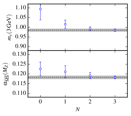
We tested the reliability of our error estimates for the perturbation theory by refitting our data using only a subset of the known perturbative coefficients. The results are presented in Fig. 4, which shows values for $m_{c}(3\,\mathrm{GeV})$ and $\alpha_{\mathrm{\overline{MS}}}(M_{Z})$ from fits that treat perturbative coefficients beyond order $N$ as fit parameters, with priors as in Eq. (24). Results from different orders agree with each other, providing evidence that our estimates of truncation errors are reliable. This plot also shows the steady convergence of perturbation theory as additional orders are added.

As a further test of perturbation theory, we refit our nonperturbative data treating the leading perturbative coefficients, $\gamma_{0}$ and $\beta_{0}$ , in the evolution equations for the mass (Eq. (21)) and coupling (Eq. (20)) as fit parameters with priors of $0\pm 1$ . The fit gives

\gamma_{0}=0.292(19)\quad\quad\beta_{0}=0.675(54),

(41)

in good agreement with the exact results of $0.318$ and $0.663$ , respectively. So our nonperturbative results for the correlators show clear evidence for the evolution of $m_{c}(\mu)$ and $\alpha_{\mathrm{\overline{MS}}}(\mu)$ as $\mu=3m_{h}$ varies from $3m_{c}$ to $9m_{c}$ .

III $m_{c}/m_{s}$ from $n_{f}=4$

As discussed above (Section II.1), we can use lattice QCD to extract ratios of $\mathrm{\overline{MS}}$ quark masses completely nonperturbatively [32], since ratios of quark masses are scheme and scale independent: for example,

\left.\frac{m_{0c}}{m_{0s}}\right|_{\mathrm{lat}}=\left.\frac{m_{c}(\mu,n_{f})}{m_{s}(\mu,n_{f})}\right|_{\mathrm{\overline{MS}}}+{\cal O}((am_{c})^{2}\alpha_{s}).

(42)

While ratios of light-quark masses can be obtained from chiral perturbation theory, only lattice QCD can produce nonperturbative ratios involving heavy quarks. These ratios are very useful for checking mass determinations that rely upon perturbation theory, as illustrated in [2]. They also allow us to leverage precise values of light-quark masses from very accurately determined heavy-quark masses.

In [32] we used nonperturbative simulations, with $n_{f}=3$ sea quarks, to determine the $s$ quark’s mass from the $c$ quark’s mass and the ratio $m_{c}/m_{s}$ . We repeat that analysis here, but now for $n_{f}=4$ sea quarks, using the tuned values of the bare $s$ and $c$ masses for each of our lattice ensembles: $am_{0s}^{\mathrm{tuned}}$ and $am_{0c}^{\mathrm{tuned}}$ in Table 2, respectively. We expect

	$\displaystyle\frac{am_{0c}^{\mathrm{tuned}}}{am_{0s}^{\mathrm{tuned}}}=$	$\displaystyle\,\frac{m_{c}}{m_{s}}\left(1+h_{m}\frac{\delta m_{uds}^{\mathrm{sea}}}{m_{s}}+h_{a^{2},m}\frac{\delta m_{uds}^{\mathrm{sea}}}{m_{s}}\left(\frac{m_{c}}{\pi/a}\right)^{2}\right.$
		$\displaystyle\left.+h_{1}\alpha_{s}(\pi/a)\left(\frac{m_{c}}{\pi/a}\right)^{2}+\sum_{j=2}^{N_{a^{2}}}h_{j}\left(\frac{m_{c}}{\pi/a}\right)^{2j}\right),$		(43)

where again we ignore $\delta m_{c}^{\mathrm{sea}}$ and $\delta m^{2}$ dependence since they are negligible. We fit the data from Table 2 using this formula with the following fit parameters and priors:

	$\displaystyle h_{m}$	$\displaystyle=0\pm 0.1,$	$\displaystyle h_{a^{2},m}$	$\displaystyle=0\pm 0.1,$		(44)
	$\displaystyle h_{1}$	$\displaystyle=0\pm 6,$	$\displaystyle h_{j}$	$\displaystyle=0\pm 2\quad(j>1).$		(45)

The extrapolated value $m_{c}/m_{s}$ is also a fit parameter. We set $N_{a^{2}}=5$ , but get identical results for any $N_{a^{2}}\geq 2$ .

The result of this fit is presented in Fig. 5, which shows the $a^{2}$ dependence of the lattice results. The sensitivity of our new results to $a^{2}$ is about half what we saw in our previous analysis. Our new fit is excellent and gives a final result for the mass ratio of:

\frac{m_{c}(\mu,n_{f})}{m_{s}(\mu,n_{f})}=11.652(65).

(46)

The leading sources of error in this result are listed in Table 4. These are dominated by statistical errors and uncertainty in the $\eta_{s}$ mass. Many other potential sources of error, such as uncertainties in the lattice spacing, largely cancel in the ratio.

Note that the discussion in Appendix A and Eq. (78), in particular, imply that the leading effect of mistuned sea-quark masses cancels in ratios of quark masses. This is substantiated by our fit which makes parameter $h_{m}$ negligibly small ( $-0.0080(34)$ ). Setting $h_{m}=0$ shifts our result for $m_{c}/m_{s}$ by only $\sigma/7$ .

Our result is a little more than a standard deviation lower than the recent result, $11.747(19)\binom{+59}{-43}$ , computed by the Fermilab/MILC collaboration (using many of the same configurations we use) [33]. Our analysis uses a different scheme for tuning the lattice spacing and quark masses, which leads to the lack of sea-quark mass dependence in $m_{c}/m_{s}$ discussed just above. The absence of sea-mass dependence is apparent from Fig. 5, where the clusters of data points correspond to ensembles with the same bare lattice coupling but different sea-quark masses. This figure can be compared with Fig. 6 in [33], which shows much larger sea-mass dependence. Both approaches should agree when extrapolated to zero lattice spacing and the physical sea-quark masses.

IV $m_{h}/m_{c}$ from $m_{\eta_{h}}$

An analysis similar to that in the previous section allows us to relate heavy-quark masses $m_{h}$ to the $h\overline{h}$ pseudoscalar mass $m_{\eta_{h}}$ with data from Table 3. This can be used, for example, to estimate the $b$ mass by extrapolating to $m_{\eta_{b}}$ .

Here we fit the lattice mass ratios $m_{0h}/m_{0c}^{\mathrm{tuned}}$ to the following function of $m_{\eta_{h}}$ from the simulation:

	$\displaystyle\frac{m_{h}}{m_{c}}$	$\displaystyle=\frac{m_{\eta_{h}}}{m_{\eta_{c}}}\sum_{n=0}^{N}f_{n}(m_{\eta_{h}})\left(\frac{am_{\eta_{h}}}{4}\right)^{2n}$
		$\displaystyle+f_{\mathrm{sea}}(\eta_{h})\frac{m_{\eta_{h}}}{m_{\eta_{c}}}\frac{\delta m_{uds}^{\mathrm{sea}}}{m_{s}}\left(\frac{am_{\eta_{h}}}{4}\right)^{2}$		(47)

where $N=20$ , although any $N>3$ gives the same result. Here $f_{n}(m_{\eta_{h}})$ and $f_{\mathrm{sea}}(m_{\eta_{h}})$ are cubic splines with knots at

m_{\mathrm{knots}}=\{2.9,3.6,4.6,7.9\}\,\mathrm{GeV}.

(48)

The maximum and minimum knots correspond to the maximum and minimum values of $m_{\eta_{h}}$ , while the locations of the internal knots were obtained by treating those locations as fit parameters. Each $f$ is parameterized by

f(m)=f_{0}+\delta f(m)

(49)

and fit parameters

$\displaystyle f_{0}$	$\displaystyle=0\pm 1$
$\displaystyle\delta f(m)$	$\displaystyle=0\pm 0.15$	$\displaystyle\quad m$	$\displaystyle\in m_{\mathrm{knots}}$
$\displaystyle\delta f^{\prime}(m)$	$\displaystyle=0.15\pm 0.15$	$\displaystyle\quad m$	$\displaystyle=2.9\,\mathrm{GeV}.$	(50)

We reduce the priors for the leading $a^{2}$ errors by a factor of $1/3$ since these errors are suppressed by $\alpha_{s}$ in the HISQ discretization. The choice of priors for the spline parameters is motivated by results from [2] (see Figure 4 in that paper).

The fit is excellent with a $\chi^{2}$ per degree of freedom of 0.44 for 29 pieces of data: see the top panel in Figure 6. Finite lattice spacing errors are much smaller for this quantity than for the moments, and it is again largely independent of mistunings in the sea-quark masses. Extrapolating to $m_{\eta_{b}}$ gives

m_{b}/m_{c}=4.528(54)

(51)

which agrees with our $n_{f}=3$ result of $4.51(4)$ , but with larger errors [2]. Our new $n_{f}=4$ data go down to lattice spacings of $0.06$ fm; our earlier analysis also had results at $0.045$ fm.

The bottom panel of Figure 6 compares our new $n_{f}=4$ data with $n_{f}=3$ results obtained from fits to the current-current correlators [2]. The agreement is excellent, showing again that $n_{f}=3$ and $n_{f}=4$ are consistent with each other.

V Conclusions and Outlook

The initial extractions of quark masses from heavy-quark current-current correlators relied upon experimental data from $e\overline{e}$ annihilation [34, 35]. Our analysis here, like the two that preceded it [30, 2], replaces experimental data with nonperturbative results from tuned lattice simulations.

Lattice simulations offer several advantages over experiment for this kind of calculation [1]. For one thing, simulations are easier to instrument than experiments and much more flexible. Thus we can generate lattice “data” not just for vector-current correlators, but for any heavy-quark current or density; we optimize our simulations by using the pseudoscalar density instead of the vector current. Experiment provides results for only two heavy-quark masses — $m_{c}$ and $m_{b}$ — but we can produce lattice data for a whole range of masses between $m_{c}$ and $m_{b}$ . This means that $\alpha_{\mathrm{\overline{MS}}}(\mu)$ varies continuously, by almost a factor of two, in our analysis since $\mu\propto m_{h}$ . Here we use this variation to estimate and bound uncalculated terms in perturbation theory, providing much more reliable estimates of perturbative errors than the standard procedure of replacing $\mu$ by $\mu/2$ and $2\mu$ . (Our analysis is essentially independent of $\mu$ .) Nonperturbative contributions are also strongly dependent upon $m_{h}$ , and therefore more readily bound if a range of masses is available; they are negligible in our analysis.

In this paper, we have redone our earlier $n_{f}=3$ analysis [2] using simulations with $n_{f}=4$ sea quarks: $u$ , $d$ , $s$ and $c$ . Our new results,

	$\displaystyle m_{c}(3\,\mathrm{GeV},n_{f}=4)$	$\displaystyle=0.9851(63)\,\mathrm{GeV}$		(52)
	$\displaystyle\alpha_{\mathrm{\overline{MS}}}(M_{Z},n_{f}=5)$	$\displaystyle=0.11822(74),$		(53)

agree well with our earlier results of $0.986(6)$ GeV and $0.1183(7)$ , suggesting that contributions from $c$ quarks in the sea are reliably estimated using perturbation theory (as expected). Our $c$ mass is about $1.8\sigma$ lower than the recent result from the ETMC collaboration, also using $n_{f}=4$ simulations but with a different method [36]: they get $m_{c}(m_{c})=1.348(42)$ GeV, compared with our $n_{f}=4$ result of 1.2715(95) GeV.

We updated our earlier $n_{f}=3$ analysis [32] of the ratio $m_{c}/m_{s}$ of quark masses using our $n_{f}=4$ data. This is a relatively simple analysis of data from Table 2. Our new value is:

\frac{m_{c}(\mu,n_{f})}{m_{s}(\mu,n_{f})}=11.652(65).

(54)

It agrees well with our previous result $11.85(16)$ , but is much more accurate. We compare our new result with others in Fig. 7.

We obtain a new estimate for the $s$ mass by combining our new result for $m_{c}/m_{s}$ with our new estimate of the $c$ mass (Eq. (52), converted from $n_{f}=4$ ):

m_{s}(\mu,n_{f}=3)=\begin{cases}93.6(8)\,\mathrm{MeV}&\mu=2\,\mathrm{GeV}\\ 84.7(7)\,\mathrm{MeV}&\mu=3\,\mathrm{GeV}.\end{cases}

(55)

Values for $m_{s}(\mu,n_{f}=4)$ are smaller by about 0.2 MeV. Our new result agrees with our previous analysis and also with other recent $n_{f}=3$ or 4 analyses:

	$\displaystyle m_{s}(2\,\mathrm{GeV})$	$\displaystyle=\begin{cases}92.4(1.5)\,\mathrm{MeV}&\mbox{HPQCD~\cite[cite]{[\@@bibref{Number}{Davies:2009ih}{}{}]}},\\ 99.6(4.1)\,\mathrm{MeV}&\mbox{ETMC~\cite[cite]{[\@@bibref{Number}{Carrasco:2014cwa}{}{}]},}\\ 95.5(1.9)\,\mathrm{MeV}&\mbox{Durr~\emph{et al}~\cite[cite]{[\@@bibref{Number}{Durr:2010vn}{}{}]},}\\ \end{cases}$
	$\displaystyle m_{s}(3\,\mathrm{GeV})$	$\displaystyle=83.5(2.0)\,\mathrm{MeV}\quad\mbox{RBC/UKQCD~\cite[cite]{[\@@bibref{Number}{Arthur:2012opa}{}{}]}}.$		(56)

Finally, we have also updated our previous ( $n_{f}=3$ ) nonperturbative analysis of $m_{b}/m_{c}$ using our new $n_{f}=4$ data. We obtain:

\frac{m_{b}(\mu,n_{f})}{m_{c}(\mu,n_{f})}=4.528(54),

(57)

which agrees with our previous result of 4.51(4) [2]. Combining this result with our new value for $m_{c}$ (Eq. (52)) gives

m_{b}(m_{b},n_{f}=5)=4.162(48).

(58)

This again agrees with our earlier result of 4.164(23) GeV, but with larger errors. We can also multiply our results for $m_{b}/m_{c}$ and $m_{c}/m_{s}$ to obtain

\frac{m_{b}(\mu,n_{f})}{m_{s}(\mu,n_{f})}=52.55(55).

(59)

This is almost four standard deviations (but only 4%) away from the result predicted by the Georgi-Jarlskog relationship [41] for certain classes of grand unified theory: the Georgi-Jarlskog relationship says that $m_{b}/m_{s}$ should equal $3m_{\tau}/m_{\mu}=50.45$ .

The prospects for improving our results over the next decade are good. Detailed meta-simulations, described in [1], indicate that errors from our analysis can be pushed below 0.25% by a combination of higher-order perturbation theory, and, especially, smaller lattice spacings (0.045, 0.03 and 0.023 fm) — both improvements that are quite feasible over a decade [1]. There are also many other promising approaches within lattice QCD. Several exist already for extracting the QCD coupling: see, for example, [42, 43, 44, 45, 46, 47]. One can also use simulations of other renormalized quantities, such as the $m_{h}\overline{\psi}_{h}\gamma_{5}\psi$ vertex function, to compute quark masses [12].

Small lattice spacings are particularly important for the $b$ mass, because lattice spacing errors are typically of order $(am_{b})^{2}$ . One approach is to use highly-improved relativistic actions for the $b$ quarks, like the HISQ action used here. As shown in [3], all but one of the ${\cal O}(a,a^{2})$ operators that arise in the Symanzik improvement of a quark action are suppressed by extra factors of the heavy-quark velocity: factors of $(v/c)^{2}$ for mesons made of heavy quarks, and $v/c$ for mesons made of a combination of heavy and light quarks. The one operator that does not have extra suppression is $\sum_{\mu}\overline{\psi}\gamma^{\mu}(D^{\mu})^{3}\psi$ , which violates Lorentz invariance and so is easily tuned nonperturbatively using the meson dispersion relation. This is the strategy adopted in the HISQ discretization we use here. The extra factors of $v/c$ suppress $(am_{b})^{2}$ errors by an extra order of magnitude, beyond the suppression, by a power of $\alpha_{s}$ , coming from tree-level corrections for $a^{2}$ errors in HISQ.

$(am_{b})^{2}$ errors can be avoided completely by using effective field theories like NRQCD [48] or the Fermilab formalism [49] for $b$ dynamics. Such approaches should be sufficiently accurate provided they are corrected to sufficiently high order in $(v_{b}/c)^{2}$ . Our recent NRQCD analysis of $m_{b}$ , using current-current correlators, is encouraging [50].

Overall the prospects are excellent for continued improvement.

Acknowledgements.

We are grateful to the MILC collaboration for the use of their gauge configurations and code. We thank S. King and D. Toussaint for useful conversations. Our calculations were done on the Darwin Supercomputer as part of STFC’s DiRAC facility jointly funded by STFC, BIS and the Universities of Cambridge and Glasgow. This work was funded by STFC, the Royal Society, the Wolfson Foundation and the National Science Foundation.

Appendix A Sea-Quark Mass Dependence

In this appendix we discuss the dependence of the $\mathrm{\overline{MS}}$ coupling and heavy-quark masses on the sea-quark masses. We vary the $u/d$ sea-quark mass in our simulations to help us assess systematic errors associated with tuning that mass. In addition, the precision with which the $s$ and $c$ sea-quark masses have been tuned varies by several percent over the various ensembles we use. These detunings shift the $\mathrm{\overline{MS}}$ coupling and masses. We need to understand how they are shifted in order to extract results for $\alpha_{\mathrm{\overline{MS}}}$ and $m_{h}$ with physical sea-quark masses.

It is essential when discussing detuned sea-quark masses to be specific about what is held fixed as the quark masses are shifted from their physical values. An obvious choice is to fix both the lattice spacing $a$ and the bare coupling $\alpha_{\mathrm{lat}}$ in the lattice lagrangian, while varying the quark masses. We find it more convenient, however, to explore a slightly different manifold in theory space by fixing $\alpha_{\mathrm{lat}}$ and the value of the Wilson-flow parameter $w_{0}$ .

Lattice simulations are done for particular values of the bare coupling constant (and bare quark masses), but with all dimensional quantities expressed in units of the lattice spacing (lattice units). This removes explicit dependence on the lattice spacing from the simulation, so we can run the simulation without knowing the lattice spacing. To extract physics, however, we must determine the lattice spacing (from the simulation) and convert all simulation results from lattice units to physical units. In our simulations, we calculate the lattice spacing by measuring the value of $a/w_{0}$ in the simulation, and multiplying it by the known value of $w_{0}$ for physical sea-quark masses (that is, 0.1715(9) fm). As a result the lattice spacing becomes (weakly) dependent upon the sea-quark masses since $w_{0}$ is affected by sea quarks.

This procedure is convenient because the lattice spacing for a given ensemble is determined using information from only that ensemble, thereby decoupling the analyses of different ensembles to a considerable extent. As we discuss below there is an added benefit when vacuum polarization from $c$ (or heavier) quarks is included in the simulation, as we do here: heavy quarks automatically decouple from low-energy physics (like $w_{0}$ [*[Perturbationtheorysuggeststhattheimportantscalesin~$w_0$areoforder$Q_w_0=1/\sqrt{8w^2_0}≈400$MeV.See][]Luscher:2010iy]). With our procedure, physical quantities that probe energy scales smaller than $2m_{c}$ — that is, almost everything studied with lattice QCD today — are essentially independent of $m_{c}$ , which means that they are completely unaffected by tuning errors in $m_{c}$ . This would not be the case if we fixed the lattice spacing instead of $w_{0}$ , since it is small variations in the lattice spacing that correct for mistuning in $m_{c}$ .

It is also very convenient that we set the lattice spacing using a flavor singlet quantity. Because $w_{0}$ is a flavor singlet, the leading sea-mass dependence induced in the lattice spacing is analytic (linear) in the quark mass and small; in particular, there are no chiral logarithms [52]. One consequence is that leading-order chiral perturbation theory for physical quantities ( $f_{\pi}$ , $f_{D_{s}}$ …) is unchanged from standard treatments except for shifts (that are easily accommodated) in the coefficients of certain analytic terms.

In this appendix we show how the $\mathrm{\overline{MS}}$ coupling and heavy-quark mass depend upon the sea-quark masses in our simulations. This dependence implies sea-quark mass dependence in the lattice spacing and the heavy quark’s bare mass, which we then use to determine some of the parameters involved. Finally we review heavy-quark decoupling, and estimate the parameters for $c$ -mass dependence using first-order perturbation theory.

A.1 Tuning Bare Quark Masses

We define tuned values for the bare $c$ and $s$ masses on each ensemble by adjusting those masses to give physical values in simulations for the $\eta_{c}$ and $\eta_{s}$ masses. The tuned values are listed in Table 2.

The current experimental value for the $\eta_{c}$ mass is 2.9836(7) GeV [28]. In our analysis, we remove electromagnetic corrections from this value, and adjust its error to account for $c\overline{c}$ annihilation, since neither effect is in our simulations [53, 54]. We use:

m_{\eta_{c}}^{\mathrm{phys}}=2.9863(27)\,\mathrm{GeV}.

(60)

We compute the tuned $c$ mass $m_{0c}^{\mathrm{tuned}}$ by linear interpolation using $\eta_{h}$ masses from the simulation (Table 3) for heavy-quark masses $m_{0h}$ in the vicinity of $m_{0c}$ . In a few cases we have results for only a single value of $m_{0h}$ ; then we compute the tuned $c$ mass using estimates of $dm_{\eta_{c}}/dm_{0c}$ from other ensembles with (almost) the same lattice spacing.

Note that the uncertainty in $m_{0c}^{\mathrm{tuned}}$ is usually smaller than that in $am_{0c}^{\mathrm{tuned}}$ . This is a peculiar feature of heavy-quark masses in lattice simulations (see, for example, [55]). It follows from the formula for the linear interpolation that defines the tuned mass in terms of a nearby mass:

m_{0c}^{\mathrm{tuned}}=(am_{0c})a^{-1}+\frac{dm_{0c}}{dm_{\eta_{c}}}\left(m_{\eta_{c}}^{\mathrm{phys}}-(am_{\eta_{c}})a^{-1}\right)

(61)

where $am_{\eta_{c}}$ is the simulation result for the $\eta_{c}$ mass (in lattice units) when the $c$ quark has mass $am_{0c}$ . Here $dm_{0c}/dm_{\eta_{c}}$ is obtained from simulation results for a few nearby $c$ masses. The uncertainty in $a^{-1}$ is usually larger than the uncertainties in the other lattice quantities, but here $a^{-1}$ is multiplied by

(am_{0c})-(am_{\eta_{c}})\frac{dm_{0c}}{dm_{\eta_{c}}}

(62)

which would vanish if $m_{\eta_{c}}=2m_{0c}$ . This cancellation is only partial for real masses, but it doesn’t occur at all if Eq. (61) is multiplied on both sides by $a$ to give a formula for $am_{0c}^{\mathrm{tuned}}$ . As a result, fractional errors are roughly $3\times$ smaller for $m_{0c}^{\mathrm{tuned}}$ .

The $\eta_{s}$ is an $s\overline{s}$ pseudoscalar particle where the valence quarks are (artificially) not allowed to annihilate; its physical mass is determined in lattice simulations from the masses of the pion and kaon [17]:

m_{\eta_{s}}^{\mathrm{phys}}=0.6885(22)\,\mathrm{GeV}

(63)

This mass is defined for use in lattice simulations and needs no further corrections for electromagnetism. We tune the $s$ mass by simulating with a nearby bare mass $m_{0s}$ to obtain the corresponding $\eta_{s}$ mass, and then extracting the tuned mass using:

m_{0s}^{\mathrm{tuned}}=m_{0s}\left(\frac{m_{\eta_{s}}^{\mathrm{phys}}}{m_{\eta_{s}}}\right)^{2}.

(64)

Our $\eta_{s}$ data are presented in Table 5, which shows that the tuned mass is quite insensitive to small variations in $m_{0s}$ . We do not have $\eta_{s}$ results for ensemble 7; there the tuned $s$ mass is based on an interpolation between results from ensemble 8 and another ensemble that has similar parameters but with $am_{0\ell}=0.0074$ .

Table 2 shows that $m_{0c}^{\mathrm{tuned}}$ is more accurate than $m_{0s}^{\mathrm{tuned}}$ . This is because the uncertainties in the value of the lattice spacing have a smaller impact on the $c$ mass because the cancellation described above only happens for heavy quarks (where $m_{\eta_{h}}\approx 2m_{0h}$ ).

Table 5: Simulation results for the

\eta_{s}

mass

am_{\eta_{s}}

corresponding to different values of the bare

s

mass

am_{0s}

and different gluon ensembles. The ensembles are described in Table 2, although we use many more configurations for our

\eta_{s}

analysis than are indicated there. Estimates for the tuned bare

s

mass (Eq. (64)) are also given.

ensemble	$am_{0s}$	$\quad am_{\eta_{s}}$	$am_{0s}^{\mathrm{tuned}}$
1	0.0705	0.54024(15)	0.0700(9)
	0.0688	0.53350(17)	0.0700(9)
	0.0641	0.51511(16)	0.0700(9)
2	0.0679	0.52798(9)	0.0686(8)
	0.0636	0.51080(9)	0.0687(8)
3	0.0678	0.52680(8)	0.0677(8)
4	0.0541	0.43138(12)	0.0545(7)
	0.0522	0.42358(11)	0.0545(7)
5	0.0533	0.42637(6)	0.0533(7)
	0.0507	0.41572(14)	0.0534(7)
	0.0505	0.41474(8)	0.0534(7)
6	0.0527	0.42310(3)	0.0527(6)
	0.0507	0.41478(4)	0.0527(6)
8	0.0360	0.30480(4)	0.0364(4)
9	0.0231	0.20549(8)	0.0234(3)

We set the $u$ and $d$ masses equal to their average,

m_{\ell}\equiv\frac{m_{u}+m_{d}}{2},

(65)

and set $m_{\ell}$ equal to the tuned $s$ mass (above) divided by the physical value of the quark mass ratio [33]

\frac{m_{s}}{m_{\ell}}=27.35(11).

(66)

A.2 $\alpha_{\mathrm{\overline{MS}}}(\mu,\delta m^{\mathrm{sea}})$ and $a(\delta m^{\mathrm{sea}})$

The beta function in the $\mathrm{\overline{MS}}$ scheme is, by definition, independent of sea-quark masses. Thus the coupling’s evolution is unchanged by detuned sea-quark masses —

\frac{d\alpha_{\mathrm{\overline{MS}}}(\mu,\delta m^{\mathrm{sea}})}{d\log\mu^{2}}=\beta(\alpha_{\mathrm{\overline{MS}}}(\mu,\delta m^{\mathrm{sea}}))

(67)

— but mass dependence enters through the low-energy starting point for that evolution implied by the scale-setting procedure used in the lattice simulation. Such mass dependence can enter only through an overall renormalization of the scale parameter $\mu$ :

\alpha_{\overline{\mathrm{MS}}}(\mu,\delta m^{\mathrm{sea}})=\alpha_{\mathrm{\overline{MS}}}(\xi_{\alpha}\mu)

(68)

where

\displaystyle\alpha_{\mathrm{\overline{MS}}}(\mu)

\displaystyle\equiv\alpha_{\mathrm{\overline{MS}}}(\mu,\delta m^{\mathrm{sea}}=0)

(69)

is the $\mathrm{\overline{MS}}$ coupling for physical sea-quark masses. The scale factor,

	$\displaystyle\xi_{\alpha}\equiv 1$	$\displaystyle+g_{\alpha}\frac{\delta m_{uds}^{\mathrm{sea}}}{m_{s}}+g_{a^{2},\alpha}\frac{\delta m_{uds}^{\mathrm{sea}}}{m_{s}}\left(\frac{m_{c}}{\pi/a}\right)^{2}$
		$\displaystyle+g_{c,\alpha}\frac{\delta m_{c}^{\mathrm{sea}}}{m_{c}}+{\cal O}(\delta m^{2}),$		(70)

depends upon the differences between the masses $m_{q}$ used in the simulation and the tuned values of those masses $m_{q}^{\mathrm{tuned}}$ (Table 2 and Sec. A.1):

	$\displaystyle\delta m_{uds}^{\mathrm{sea}}$	$\displaystyle\equiv\sum_{q=u,d,s}\left(m_{q}-m_{q}^{\mathrm{tuned}}\right)$		(71)
	$\displaystyle\delta m_{c}^{\mathrm{sea}}$	$\displaystyle\equiv m_{c}-m_{c}^{\mathrm{tuned}}.$		(72)

Function $\alpha_{\mathrm{\overline{MS}}}(\xi_{\alpha}\mu)$ satisfies the standard evolution equation (Eq. (67)) because $\xi_{\alpha}$ is independent of $\mu$ .

We work to first order in $\delta m^{\mathrm{sea}}$ because higher-order terms are negligible in our simulations. As suggested above, he leading-order dependence is particularly simple because we use iso-singlet mesons ( $\eta_{c}$ and $\eta_{s}$ ) to set the $c$ and $s$ masses; in particular, there are no chiral logarithms of the $u/d$ mass in leading order.

We expect coefficients $g_{\alpha}$ and $g_{a^{2},\alpha}$ in $\xi_{\alpha}$ to be of order $1/10$ since corrections linear in light-quark masses must be due to chiral symmetry breaking and so should be of order $\delta m^{sea}/\Lambda$ where $\Lambda\approx 10m_{s}$ . As we discuss below, $g_{c,\alpha}$ can be estimated from perturbation theory and is again of order $1/10$ . We treat these coefficients as fit parameters in our analysis, with priors:

g_{\alpha}=0\pm 0.1,\quad g_{a^{2},\alpha}=0\pm 0.1,\quad g_{c,\alpha}=0\pm 0.1.

(73)

The rescaling factor $\xi_{\alpha}$ is closely related to the dependence of the lattice spacing on the sea-quark masses used in the simulation. The lattice spacing is primarily a function of the bare coupling $\alpha_{\mathrm{lat}}$ used in the lattice action, but it also varies with the sea-quark masses, in our scheme, when the bare coupling is held constant. As discussed above, this is because of sea-mass dependence in the quantity used to define the lattice spacing, $a/w_{0}$ in our case. The relationship with $\xi_{\alpha}$ can be understood by examining the $\mathrm{\overline{MS}}$ coupling at scale $\mu=\pi/a$ . There it is related to the bare coupling by a perturbative expansion,

	$\displaystyle\alpha_{\mathrm{\overline{MS}}}(\pi/a,\delta m^{\mathrm{sea}})$	$\displaystyle=\alpha_{\mathrm{\overline{MS}}}(\xi_{\alpha}\pi/a)$
		$\displaystyle=\alpha_{\mathrm{lat}}+\sum_{n=2}^{\infty}c_{n}^{\mathrm{\overline{MS}}}\,\alpha_{\mathrm{lat}}^{n},$		(74)

that is mass-independent up to corrections of ${\cal O}((am_{c})^{2}\alpha_{s})$ , which are negligible in our analysis. This formula implies that $\alpha_{\mathrm{\overline{MS}}}(\xi_{\alpha}\pi/a)$ is constant if $\alpha_{\mathrm{lat}}$ is, and therefore that $\xi_{\alpha}/a$ must be constant as well. Consequently the lattice spacing must vary with $\delta m^{\mathrm{sea}}$ like

\displaystyle a(\delta m^{\mathrm{sea}})\approx\xi_{\alpha}\,a_{\mathrm{phys}}

(75)

if the bare coupling is held constant, where $a_{\mathrm{phys}}$ is the lattice spacing when the sea-quark masses are tuned to their physical values — that is, $a_{\mathrm{phys}}\equiv a(\delta m^{\mathrm{sea}}=0)$ .

We use this variation in the lattice spacing to read off the parameters in $\xi_{\alpha}$ . Our simulation results fall into four groups of gluon ensembles, with lattice spacings around 0.15 fm, 0.12 fm, 0.09 fm and 0.06 fm. Each group corresponds to a single value of the bare lattice coupling $\alpha_{\mathrm{lat}}$ , and several different values of light sea-quark mass. Within a single group, then, the values we obtain for $a/w_{0}$ from our simulations should vary as

(a/w_{0})_{\mathrm{sim}}=\xi_{\alpha}\times(a/w_{0})_{\mathrm{phys}},

(76)

where the parameters $g_{\alpha}$ , $g_{a^{2},\alpha}$ and $g_{c,\alpha}$ in $\xi_{\alpha}$ (Eq. (70)) are the same for all four groups of data.

We fit our simulation results for $a/w_{0}$ , simultaneously for all four groups, as functions of $g_{\alpha}$ , $g_{a^{2},\alpha}$ and $g_{c,\alpha}$ . We also treat the value of $(a/w_{0})_{\mathrm{phys}}$ for each group as a fit parameter. The resulting fit is shown in Fig. 8 where we plot

\frac{(a/w_{0})_{\mathrm{sim}}}{(a/w_{0})_{\mathrm{phys}}}

versus $\delta m^{\mathrm{sea}}_{uds}/m_{s}$ .

The fit is excellent, and shows that $g_{\alpha}=0.082(8)$ . Our fit is not very sensitive to $g_{a^{2},\alpha}$ and $g_{c,\alpha}$ — their impact on $\xi_{\alpha}$ is too small — and gives results for these that are essentially the same as the prior values.

A.3 $m_{h}(\mu,\delta m^{\mathrm{sea}})$ and $m_{0c}(\delta m^{\mathrm{sea}})$

The evolution equations for the heavy quark’s $\mathrm{\overline{MS}}$ mass are unchanged by sea-mass detunings:

\frac{d\log(m_{h}(\mu,\delta m^{\mathrm{sea}}))}{d\log\mu^{2}}=\gamma_{m}(\alpha_{\mathrm{\overline{MS}}}(\mu,\delta m^{\mathrm{sea}}))

(77)

Consequently any sea-mass dependence must enter through rescalings:

m_{h}(\mu,\delta m^{\mathrm{sea}})=\xi_{m}m_{h}(\xi_{\alpha}\mu)

(78)

where $\xi_{\alpha}$ is defined above (Eq. (70)), $\xi_{m}$ is independent of $\mu$ , and

m_{h}(\mu)\equiv m_{h}(\mu,\delta m^{\mathrm{sea}}=0)

(79)

is the $\mathrm{\overline{MS}}$ mass for physical sea-quark masses. We parameterize $\xi_{m}$ similarly to $\xi_{\alpha}$ but allowing for the coefficients to depend upon the heavy-quark mass:

	$\displaystyle\xi_{m}=1$	$\displaystyle+\frac{g_{m}}{(m_{\eta_{h}}/m_{\eta_{c}})^{\zeta}}\frac{\delta m_{uds}^{\mathrm{sea}}}{m_{s}}$
		$\displaystyle+\frac{g_{a^{2},m}}{(m_{\eta_{h}}/m_{\eta_{c}})^{\zeta}}\frac{\delta m_{uds}^{\mathrm{sea}}}{m_{s}}\left(\frac{m_{c}}{\pi/a}\right)^{2}+\cdots$		(80)

Again we expect $g_{m}$ and $g_{a^{2},m}$ to be of order $1/10$ , and we treat them as fit parameters with priors:

g_{m}=0\pm 0.1,\quad g_{a^{2},m}=0\pm 0.1.

(81)

We parameterize the dependence on heavy-quark mass with the factors $(m_{\eta_{h}}/m_{\eta_{c}})^{\zeta}$ where $\zeta$ is a fit parameter with prior:

\zeta=0\pm 1.

(82)

The sea-mass dependence in $\xi_{m}$ comes from the quantity used to tune the heavy-quark mass in simulations. We tune these masses to give the correct physical mass for $\eta_{h}$ — that is, the mass obtained when the sea-quark masses are tuned to their physical values and the lattice spacing is set to zero. This means that any sea-mass dependence in $m_{\eta_{h}}$ is pushed into the rescaling factor $\xi_{m}$ in Eq. (78). The physical size of $\eta_{h}$ mesons decreases as $m_{\eta_{h}}$ increases, and this decreases the coupling with light sea-quarks. Thus we expect $\zeta>0$ in Eq. (80); our fit finds $\zeta=0.3(1)$ .

In principle, $\xi_{m}$ should depend upon $\delta m_{c}^{\mathrm{sea}}$ , as well as $\delta m_{uds}^{\mathrm{sea}}$ . Perturbation theory, however, indicates that this dependence is negligible in our simulations. Thus we have omitted such terms from $\xi_{m}$ . We have verified that they are negligible by comparing fits that include $\delta m_{c}^{\mathrm{sea}}$ terms with the fit without them.

The rescaling factor $\xi_{m}$ is closely related to the sea-mass dependence of the heavy quark’s bare mass, in much the same way $\xi_{\alpha}$ is related to the lattice spacing. The bare mass $m_{0h}$ is proportional to the $\mathrm{\overline{MS}}$ mass evaluated at $\mu=\pi/a$ :

	$\displaystyle m_{0h}$	$\displaystyle\propto m_{h}(\pi/a,\delta m^{\mathrm{sea}})$
		$\displaystyle\propto\xi_{m}m_{h}(\xi_{\alpha}\pi/a).$		(83)

Since $\xi_{\alpha}/a$ is sea-mass independent, we see that $m_{h0}$ is proportional to $\xi_{m}$ ,

m_{0h}(\delta m^{\mathrm{sea}})=\xi_{m}m_{0h}^{\mathrm{phys}},

(84)

when the sea-quark masses are varied while holding the bare coupling fixed.

This variation can be used to determine the parameters in $\xi_{m}$ , again in analogy to the previous section. As discussed in the previous section, our ensembles fall into four groups each corresponding to a different value of the bare coupling constant $\alpha_{\mathrm{lat}}$ . The masses $am_{0c}^{\mathrm{tuned}}$ for each ensemble in Table 2 are tuned to give the physical $\eta_{c}$ mass for that ensemble. Therefore, within each group of ensembles, we expect

am_{0c}^{\mathrm{tuned}}=\xi_{\alpha}\xi_{m}\times(am_{0c})_{\mathrm{phys}}

(85)

where $(am_{0c})_{\mathrm{phys}}$ is the value for properly tuned sea-quark masses.

We fit our simulation results for $am_{0c}^{\mathrm{tuned}}$ as functions of $g_{m}$ , $g_{a^{2},m}$ , $g_{\alpha}$ , $g_{a^{2},\alpha}$ , and $g_{c,\alpha}$ . We use best-fit values from the fit in the previous section as priors for the last three of these fit parameters. The values of $(am_{0c})_{\mathrm{phys}}$ for the different groups of ensembles are also fit parameters.

The resulting fit is shown in Fig. 9, where we plot $am_{0c}^{\mathrm{tuned}}/(am_{0c})_{\mathrm{phys}}$ as a function of $\delta m_{uds}^{\mathrm{sea}}/m_{s}$ . The fit is excellent and shows that $g_{m}=0.035(5)$ , while $g_{a^{2},m}$ is essentially unchanged from its prior value (because our data are not sufficiently accurate).

A.4 $c$ Quarks and Decoupling

Heavy quarks decouple from low-energy physics, and therefore variations in $\delta m_{c}^{\mathrm{sea}}$ should have no impact on physics (like $w_{0}$ ) that probes momentum scales smaller than $m_{c}$ . We can, however, introduce (apparent) violations of the decoupling theorem through the scheme used to set the lattice spacing. In particular, decoupling is violated by any scheme that holds the lattice spacing fixed (together with the bare coupling $\alpha_{\mathrm{lat}}$ ) as $\delta m_{c}^{\mathrm{sea}}$ is varied. On the contrary, decoupling is preserved by schemes that hold a low-energy ( $<2m_{c}$ ) quantity like $w_{0}$ fixed, instead of the lattice spacing ¹¹ 1 Dimensionless ratios of low-energy quantities are independent of the lattice-spacing scheme, and must be independent of $m_{c}$ by the decoupling theorem. This means that a scheme that makes any one low-energy quantity — for example, $w_{0}$ — independent of $m_{c}$ makes all other low-energy quantities independent of $m_{c}$ as well, thereby preserving decoupling..

The difference between these schemes arises because the running of the QCD coupling is modified in a detuned theory for scales between $m_{c}^{\mathrm{sea}}$ and $m_{c}^{\mathrm{sea}}+\delta m_{c}^{\mathrm{sea}}$ , resulting in a mismatch between low and high energy values of the coupling. Physics below $m_{c}$ is determined by the $n_{f}=3$ coupling constant, which, by decoupling, should be independent of $\delta m_{c}^{\mathrm{sea}}$ .

To see how this works, we examine lowest-order perturbation theory where

\alpha_{s}^{(n_{f})}(\mu)=\frac{2\pi}{\beta(n_{f})\log(\mu/\Lambda^{(n_{f})})}

(86)

with $\beta(n_{f})\equiv 11-2n_{f}/3$ , and

\displaystyle\alpha_{s}^{(3)}(\mu)=\alpha_{s}^{(4)}(\mu,\delta m_{c}^{\mathrm{sea}})

(87)

at $\mu=m_{c}+\delta m_{c}^{\mathrm{sea}}$ . Here $\Lambda^{(3)}$ must be independent of $\delta m_{c}^{\mathrm{sea}}$ , by decoupling, while $\Lambda^{(4)}$ must vary with $\delta m_{c}^{\mathrm{sea}}$ to cancel the effect of the shift in the match point $\mu=m_{c}+\delta m_{c}^{\mathrm{sea}}$ . It is straightforward to show that

	$\displaystyle\Lambda^{(4)}(\delta m_{c}^{\mathrm{sea}})$	$\displaystyle\approx m_{c}\left(\frac{\Lambda^{(3)}}{m_{c}}\right)^{\beta(3)/\beta(4)}\left(1-\frac{2}{25}\frac{\delta m_{c}^{\mathrm{sea}}}{m_{c}}\right)$
		$\displaystyle\approx\Lambda^{(4)}_{\mathrm{phys}}\times\left(1-\frac{2}{25}\frac{\delta m_{c}^{\mathrm{sea}}}{m_{c}}\right)$		(88)

where $\Lambda^{(4)}_{\mathrm{phys}}$ is the value for physical sea-quark masses. Thus the decoupling theorem requires that

\alpha_{s}^{(4)}(\mu,\delta m_{c}^{\mathrm{sea}})=\alpha_{s}^{(4)}\left(\mu\times\left(1+\frac{2}{25}\frac{\delta m_{c}^{\mathrm{sea}}}{m_{c}}\right)\right).

(89)

By comparing with Eqs. (68) and (70), we see that

g_{c,\alpha}=\frac{2}{25}+{\cal O}(\alpha_{s}),

(90)

and, therefore, that the lattice spacing varies with $\delta m_{c}^{\mathrm{sea}}$ (Eq. (75)).

There is an analogous effect in the heavy-quark mass, but the mass dependence in $\xi_{m}$ is suppressed by $\alpha_{s}^{2}$ and so is negligible in our analysis.

This analysis shows that a constant lattice spacing is incompatible with the decoupling theorem. The scheme we use avoids this problem by allowing the lattice spacing to vary with $\delta m_{c}^{\mathrm{sea}}$ , while holding the value of $w_{0}$ constant (as required by the decoupling theorem applied to $w_{0}$ itself). The violation of the decoupling theorem in the former case is only apparent; results from all schemes should agree when the sea-quark masses are tuned to their physical values.

Appendix B Previous Method

Table 6: Simulations results for

\eta_{h}

masses and reduced moments

R_{n}

(old definition) with various bare heavy-quark masses

am_{0h}

and gluon ensembles (first column, see Table 2). Data from gluon ensembles 1–3 are not listed because they were not used in the analysis in Appendix B.

	$am_{0h}$	$\quad am_{\eta_{h}}$	$R_{4}$	$R_{6}$	$R_{8}$	$R_{10}$
4	0.645	1.83976(11)	1.1842(2)	1.4857(2)	1.3785(1)	1.3179(1)
	0.663	1.87456(12)	1.1783(2)	1.4755(2)	1.3732(1)	1.3148(1)
5	0.627	1.80318(8)	1.1896(1)	1.4944(1)	1.3825(1)	1.3201(1)
	0.650	1.84797(8)	1.1819(1)	1.4813(1)	1.3759(1)	1.3162(1)
	0.800	2.13055(7)	1.1409(1)	1.4012(1)	1.3304(1)	1.2880(1)
6	0.637	1.82225(5)	1.1860(1)	1.4882(1)	1.3793(1)	1.3181(0)
7	0.439	1.34246(4)	1.2134(1)	1.5122(1)	1.3758(1)	1.3089(0)
	0.500	1.47051(4)	1.1886(1)	1.4782(1)	1.3586(1)	1.2968(0)
	0.600	1.67455(4)	1.1565(1)	1.4282(1)	1.3334(0)	1.2801(0)
	0.700	1.87210(4)	1.1315(0)	1.3827(0)	1.3089(0)	1.2647(0)
	0.800	2.06328(3)	1.1118(0)	1.3401(0)	1.2834(0)	1.2482(0)
8	0.433	1.32929(3)	1.2160(1)	1.5153(1)	1.3772(0)	1.3099(0)
	0.500	1.47012(3)	1.1885(0)	1.4777(1)	1.3582(0)	1.2965(0)
	0.600	1.67418(3)	1.1564(0)	1.4279(0)	1.3331(0)	1.2799(0)
	0.700	1.87177(2)	1.1315(0)	1.3824(0)	1.3087(0)	1.2645(0)
	0.800	2.06297(2)	1.1117(0)	1.3399(0)	1.2832(0)	1.2480(0)
9	0.269	0.88525(5)	1.2401(4)	1.5182(4)	1.3711(2)	1.3046(2)
	0.274	0.89669(5)	1.2368(4)	1.5139(3)	1.3686(2)	1.3028(1)
	0.400	1.17560(5)	1.1752(2)	1.4312(2)	1.3199(1)	1.2660(1)
	0.500	1.38750(4)	1.1440(2)	1.3854(2)	1.2943(1)	1.2465(1)
	0.600	1.59311(4)	1.1204(1)	1.3464(1)	1.2734(1)	1.2316(1)
	0.700	1.79313(4)	1.1018(1)	1.3107(1)	1.2535(1)	1.2183(1)
	0.800	1.98751(3)	1.0867(1)	1.2771(1)	1.2328(0)	1.2046(0)

The analysis in our previous ( $n_{f}=3$ ) paper used a different definition for the reduced moments with $n\geq 6$ :

R_{n\geq 6}=\frac{m_{\eta_{h}}}{2m_{0h}}\left(G_{n}/G_{n}^{(0)}\right)^{1/(n-4)}

(91)

instead of Eq. (3). As a result these moments equal $z(m_{\eta_{h}},\mu)\,r_{n}(\alpha_{\mathrm{\overline{MS}}},\mu)$ in perturbation theory where

z(m_{\eta_{c}},\mu)\equiv\frac{m_{\eta_{h}}}{2m_{h}(\mu)}

(92)

replaces $z_{c}(\mu)$ , which is defined at the $c$ mass instead of $m_{h}$ . Fits to these moments give both the coupling and the function $z(m_{\eta_{h}},\mu)$ , from which the $c$ and $b$ masses can be extracted.

We analyzed our data using the old definition, parameterizing the $m_{\eta_{h}}$ dependence of $z(m_{\eta_{c}},\mu)$ with a cubic spline. The values for the $R_{n}$ moments used are given in Table 6. We obtained results that agree with the results obtained from our new method to within a standard deviation, but are not quite as accurate:

	$\displaystyle\alpha_{\mathrm{\overline{MS}}}(5\,\mathrm{GeV},n_{f}=4)$	$\displaystyle=0.2148(29)$		(93)
	$\displaystyle m_{c}(3\,\mathrm{GeV},n_{f}=4)$	$\displaystyle=0.9896(69).$		(94)

The older method is more complicated because it attempts to determine the coupling at the same time as it determines the functional dependence of $z(m_{\eta_{h}},\mu=3m_{h})$ . In the new method, $z(m_{\eta_{h}},\mu=3m_{h})$ is replaced by $z_{c}(\mu)$ , whose dependence on $\mu$ is known a priori from perturbative QCD.

References

[1] G. P. Lepage, P. B. Mackenzie, and M. E. Peskin, (2014), arXiv:1404.0319 [hep-ph] .
[2] C. McNeile, C. Davies, E. Follana, K. Hornbostel, and G. Lepage (HPQCD Collaboration), Phys.Rev. D82, 034512 (2010), arXiv:1004.4285 [hep-lat] .
[3] E. Follana et al. (HPQCD Collaboration, UKQCD Collaboration), Phys.Rev. D75, 054502 (2007), arXiv:hep-lat/0610092 [hep-lat] .
[4] A. Hart, G. von Hippel, and R. Horgan (HPQCD Collaboration), Phys.Rev. D79, 074008 (2009), arXiv:0812.0503 [hep-lat] .
[5] M. A. Shifman, A. Vainshtein, and V. I. Zakharov, Nucl.Phys. B147, 385 (1979).
[6] K. Chetyrkin, J. H. Kuhn, and C. Sturm, Eur.Phys.J. C48, 107 (2006), arXiv:hep-ph/0604234 [hep-ph] .
[7] R. Boughezal, M. Czakon, and T. Schutzmeier, Phys.Rev. D74, 074006 (2006), arXiv:hep-ph/0605023 [hep-ph] .
[8] A. Maier, P. Maierhofer, and P. Marqaurd, Phys.Lett. B669, 88 (2008), arXiv:0806.3405 [hep-ph] .
[9] Y. Kiyo, A. Maier, P. Maierhofer, and P. Marquard, Nucl.Phys. B823, 269 (2009), arXiv:0907.2120 [hep-ph] .
[10] A. Maier, P. Maierhofer, P. Marquard, and A. Smirnov, Nucl.Phys. B824, 1 (2010), arXiv:0907.2117 [hep-ph] .
[11] D. J. Broadhurst, P. Baikov, V. Ilyin, J. Fleischer, O. Tarasov, et al., Phys.Lett. B329, 103 (1994), arXiv:hep-ph/9403274 [hep-ph] .
[12] G. Martinelli, C. Pittori, C. T. Sachrajda, M. Testa, and A. Vladikas, Nucl.Phys. B445, 81 (1995), arXiv:hep-lat/9411010 [hep-lat] .
[13] A. Bazavov et al. (MILC collaboration), Phys.Rev. D82, 074501 (2010), arXiv:1004.0342 [hep-lat] .
[14] A. Bazavov et al. (MILC Collaboration), Phys.Rev. D87, 054505 (2013), arXiv:1212.4768 [hep-lat] .
[15] G. Lepage, B. Clark, C. Davies, K. Hornbostel, P. Mackenzie, et al., Nucl.Phys.Proc.Suppl. 106, 12 (2002), arXiv:hep-lat/0110175 [hep-lat] .
[16] S. Borsanyi, S. Durr, Z. Fodor, C. Hoelbling, S. D. Katz, et al., JHEP 1209, 010 (2012), arXiv:1203.4469 [hep-lat] .
[17] R. Dowdall, C. Davies, G. Lepage, and C. McNeile (HPQCD Collaboration), Phys.Rev. D88, 074504 (2013), arXiv:1303.1670 [hep-lat] .
[18] T. van Ritbergen, J. Vermaseren, and S. Larin, Phys.Lett. B400, 379 (1997), arXiv:hep-ph/9701390 [hep-ph] .
[19] M. Czakon, Nucl.Phys. B710, 485 (2005), arXiv:hep-ph/0411261 [hep-ph] .
[20] J. Vermaseren, S. Larin, and T. van Ritbergen, Phys.Lett. B405, 327 (1997), arXiv:hep-ph/9703284 [hep-ph] .
[21] K. Chetyrkin, Phys.Lett. B404, 161 (1997), arXiv:hep-ph/9703278 [hep-ph] .
[22] V. Novikov, M. A. Shifman, A. Vainshtein, and V. I. Zakharov, Nucl.Phys. B249, 445 (1985).
[23] M. A. Shifman, Prog.Theor.Phys.Suppl. 131, 1 (1998), arXiv:hep-ph/9802214 [hep-ph] .
[24] M. Shifman, (2013), arXiv:1310.1966 [hep-th] .
[25] S. Hollands and C. Kopper, Commun.Math.Phys. 313, 257 (2012), arXiv:1105.3375 [hep-th] .
[26] D. Pappadopulo, S. Rychkov, J. Espin, and R. Rattazzi, Phys.Rev. D86, 105043 (2012), arXiv:1208.6449 [hep-th] .
[27] K. Chetyrkin, B. A. Kniehl, and M. Steinhauser, Nucl.Phys. B510, 61 (1998), arXiv:hep-ph/9708255 [hep-ph] .
[28] K. Olive et al. (Particle Data Group), Chin.Phys. C38, 090001 (2014).
[29] C. McNeile, A. Bazavov, C. Davies, R. Dowdall, K. Hornbostel, et al., Phys.Rev. D87, 034503 (2013), arXiv:1211.6577 [hep-lat] .
[30] I. Allison et al., Phys.Rev. D78, 054513 (2008), arXiv:0805.2999 [hep-lat] .
[31] C. Bouchard, G. P. Lepage, C. Monahan, H. Na, and J. Shigemitsu, (2014), arXiv:1406.2279 [hep-lat] .
[32] C. Davies, C. McNeile, K. Wong, E. Follana, R. Horgan, et al. (HPQCD Collaboration), Phys.Rev.Lett. 104, 132003 (2010a), arXiv:0910.3102 [hep-ph] .
[33] A. Bazavov et al. (Fermilab Lattice and MILC Collaborations), (2014), arXiv:1407.3772 [hep-lat] .
[34] K. Chetyrkin, J. Kuhn, A. Maier, P. Maierhofer, P. Marquard, et al., Phys.Rev. D80, 074010 (2009), arXiv:0907.2110 [hep-ph] .
[35] K. Chetyrkin, J. Kuhn, A. Maier, P. Maierhofer, P. Marquard, et al., Theor.Math.Phys. 170, 217 (2012), arXiv:1010.6157 [hep-ph] .
[36] N. Carrasco, A. Deuzeman, P. Dimopoulos, R. Frezzotti, V. Gimenez, et al., (2014), arXiv:1403.4504 [hep-lat] .
[37] S. Durr and G. Koutsou, Phys.Rev.Lett. 108, 122003 (2012), arXiv:1108.1650 [hep-lat] .
[38] B. Blossier et al. (ETM Collaboration), Phys.Rev. D82, 114513 (2010), arXiv:1010.3659 [hep-lat] .
[39] S. Durr, Z. Fodor, C. Hoelbling, S. Katz, S. Krieg, et al., Phys.Lett. B701, 265 (2011), arXiv:1011.2403 [hep-lat] .
[40] R. Arthur et al. (RBC Collaboration, UKQCD Collaboration), Phys.Rev. D87, 094514 (2013), arXiv:1208.4412 [hep-lat] .
[41] H. Georgi and C. Jarlskog, Phys.Lett. B86, 297 (1979).
[42] C. Davies et al. (HPQCD Collaboration), Phys.Rev. D78, 114507 (2008), arXiv:0807.1687 [hep-lat] .
[43] E. Shintani, S. Aoki, H. Fukaya, S. Hashimoto, T. Kaneko, et al., Phys.Rev. D82, 074505 (2010), arXiv:1002.0371 [hep-lat] .
[44] A. Bazavov, N. Brambilla, X. Garcia i Tormo, P. Petreczky, J. Soto, et al., Phys.Rev. D86, 114031 (2012), arXiv:1205.6155 [hep-ph] .
[45] K. Jansen, F. Karbstein, A. Nagy, and M. Wagner (ETM Collaboration), JHEP 1201, 025 (2012), arXiv:1110.6859 [hep-ph] .
[46] P. Fritzsch, F. Knechtli, B. Leder, M. Marinkovic, S. Schaefer, et al., Nucl.Phys. B865, 397 (2012), arXiv:1205.5380 [hep-lat] .
[47] B. Blossier et al. (ETM Collaboration), Phys.Rev. D89, 014507 (2014), arXiv:1310.3763 [hep-ph] .
[48] A. Lee et al. (HPQCD Collaboration), Phys.Rev. D87, 074018 (2013), arXiv:1302.3739 [hep-lat] .
[49] A. X. El-Khadra, A. S. Kronfeld, and P. B. Mackenzie, Phys.Rev. D55, 3933 (1997), arXiv:hep-lat/9604004 [hep-lat] .
[50] B. Colquhoun, R. Dowdall, C. Davies, K. Hornbostel, and G. Lepage (HPQCD Collaboration), (2014), arXiv:1408.5768 [hep-lat] .
[51] M. Luscher, JHEP 1008, 071 (2010), arXiv:1006.4518 [hep-lat] .
[52] O. Bär and M. Golterman, Phys.Rev. D89, 034505 (2014), arXiv:1312.4999 [hep-lat] .
[53] C. Davies, C. McNeile, E. Follana, G. Lepage, H. Na, et al. (HPQCD Collaboration), Phys.Rev. D82, 114504 (2010b), arXiv:1008.4018 [hep-lat] .
[54] E. B. Gregory, C. T. Davies, I. D. Kendall, J. Koponen, K. Wong, et al. (HPQCD Collaboration), Phys.Rev. D83, 014506 (2011), arXiv:1010.3848 [hep-lat] .
[55] C. Davies, K. Hornbostel, A. Langnau, G. Lepage, A. Lidsey, et al., Phys.Rev.Lett. 73, 2654 (1994), arXiv:hep-lat/9404012 [hep-lat] .
[56] Dimensionless ratios of low-energy quantities are independent of the lattice-spacing scheme, and must be independent of $m_{c}$ by the decoupling theorem. This means that a scheme that makes any one low-energy quantity—for example, $w_{0}$ —independent of $m_{c}$ makes all other low-energy quantities independent of $m_{c}$ as well, thereby preserving decoupling.

High-precision quark masses and QCD coupling from nf=4n_{f}=4 lattice QCD

Abstract

pacs

I Introduction

II Lattice Results

II.1 Heavy-Quark Correlator Moments

II.2 Lattice Simulations

II.3 Fitting Lattice Data

II.3.1 Detuned Sea-quark Masses

II.3.2 μ\mu Dependence

II.3.3 Truncated Perturbation Theory

II.3.4 Nonperturbative Effects; Finite-Volume Corrections

II.3.5 m0​h−m0​cm_{0h}-m_{0c} Correction

II.3.6 Finite Lattice Spacing Errors

II.4 nf=4n_{f}=4 Lattice Results

III mc/msm_{c}/m_{s} from nf=4n_{f}=4

IV mh/mcm_{h}/m_{c} from mηhm_{\eta_{h}}

V Conclusions and Outlook

Acknowledgements.

Appendix A Sea-Quark Mass Dependence

A.1 Tuning Bare Quark Masses

A.2 αMS¯​(μ,δ​msea)\alpha_{\mathrm{\overline{MS}}}(\mu,\delta m^{\mathrm{sea}}) and a⁡(δ​msea)a(\delta m^{\mathrm{sea}})

A.3 mh​(μ,δ​msea)m_{h}(\mu,\delta m^{\mathrm{sea}}) and m0​c​(δ​msea)m_{0c}(\delta m^{\mathrm{sea}})

A.4 cc Quarks and Decoupling

Appendix B Previous Method

References

High-precision quark masses and QCD coupling
from $n_{f}=4$ lattice QCD

II.3.2 $\mu$ Dependence

II.3.5 $m_{0h}-m_{0c}$ Correction

II.4 $n_{f}=4$ Lattice Results

III $m_{c}/m_{s}$ from $n_{f}=4$

IV $m_{h}/m_{c}$ from $m_{\eta_{h}}$

A.2 $\alpha_{\mathrm{\overline{MS}}}(\mu,\delta m^{\mathrm{sea}})$ and $a(\delta m^{\mathrm{sea}})$

A.3 $m_{h}(\mu,\delta m^{\mathrm{sea}})$ and $m_{0c}(\delta m^{\mathrm{sea}})$

A.4 $c$ Quarks and Decoupling