Fast Shortest Path Routing in Transportation Networks with Time-Dependent Road Speeds

The traversal time $c^{xy}(\tau)$ of arc $<xy>$ if $\tau$ is the time instant of departure from $x$ can be derived as follows ($ATT^{xy}(\tau)$ procedure²² 2 This procedure was initially proposed in [2]; the one presented in the current paper is an equivalent form of the one in [2].):

1. 1.

   Locate index $k$ such that $\tau_{k}\leq\tau<\tau_{k+1}$

2. 2.

   If ($v_{k}^{xy}\cdot(\tau_{k+1}-\tau)\geq d^{xy}$) $c^{xy}(\tau)=\frac{d^{xy}}{v_{k}^{xy}}$

   Else $\{$

3. 3.
   1. (a)
      1. i.

         $a=d^{xy}-v_{k}^{xy}\cdot(\tau_{{k}+1}-\tau)$

      2. ii.

         $k^{*}=k+1$

   2. (b)

      While ($v_{k^{*}}^{xy}\cdot(\tau_{k^{*}+1}-\tau_{k^{*}})<a$) $\{$

      1. i.

         $a\leftarrow a-v_{k^{*}}^{xy}\cdot(\tau_{{k^{*}}+1}-\tau_{k^{*}})$

      2. ii.

         ${k^{*}}\leftarrow{k^{*}}+1$ $\}$

4. 4.

   $c^{xy}(\tau)=(\tau_{{k^{*}}}-\tau)+\frac{a}{v_{k^{*}}^{xy}}$ $\}$

The necessity of the aforementioned procedure is due to the fact that a single time interval may not be enough for the derivation of the arc traversal time. This occurs when the distance that can be traversed from the time instant of departure till the end of the corresponding time interval, is less than the length of the arc.

Step 1 of the $ATT$ procedure needs $O(K)$ time, if the time intervals are checked sequentially. The order of the number of the time intervals that are checked during the while loop (step 3b) is $O(K)$. Therefore, the order of the computational complexity of the $ATT$ procedure is $O(K)$.

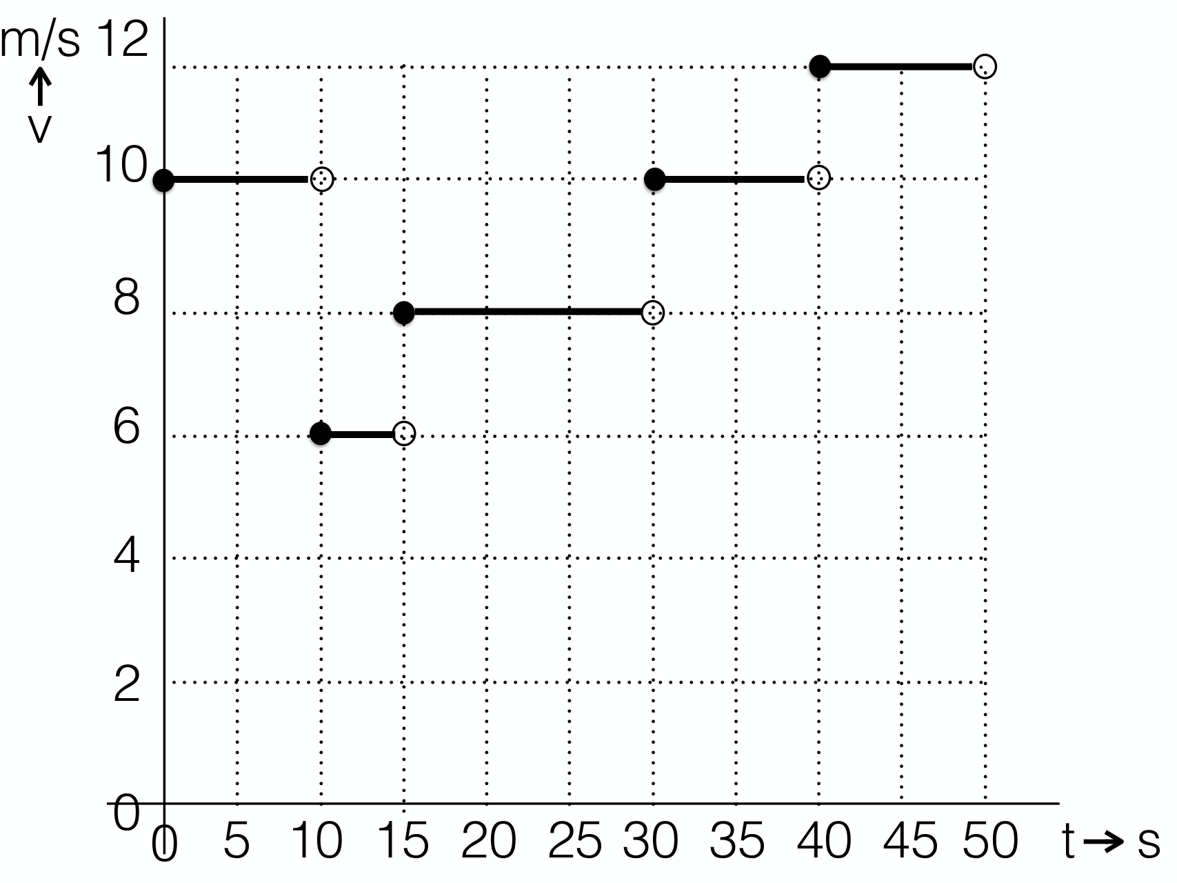
The example of Figure 1 illustrates the operation of the $ATT$ procedure. Here, the length $d^{xy}$ of arc $<xy>$ is equal to $170m$ and the departure time $\tau$ from $x$ is equal to $6s$. The first five time intervals are $[\tau_{0},\tau_{1})=[0,10)$, $[\tau_{1},\tau_{2})=[10,15)$, $[\tau_{2},\tau_{3})=[15,30)$, $[\tau_{3},\tau_{4})=[30,40)$, $[\tau_{4},\tau_{5})=[40,50)$. These along with their corresponding speed are given in Figure 1. For this example, the $ATT$ procedure performs as follows:

1. 1.

   The departure time $\tau=6s$ lies into time interval $[\tau_{0},\tau_{1})=[0,10)$ $\Rightarrow$ $k=0$

2. 2.

   The distance that can be traversed from $\tau=6s$ until the end of this time interval is equal to $v_{0}^{xy}\cdot(\tau_{1}-\tau)=10\cdot(10-6)=40m$. Since it is smaller than the length of the arc, the procedure is continued.

3. 3.
   1. (a)
      1. i.

         $a=d^{xy}-v_{0}^{xy}\cdot(\tau_{1}-\tau)=170-40=130m$

      2. ii.

         ${k^{*}}=1$

   2. (b)
      • •

        $v_{1}^{xy}\cdot(\tau_{2}-\tau_{1})=6\cdot(15-10)=30m<a=130m\Rightarrow$

        1. i.

           $a=130-30=100m$

        2. ii.

           ${k^{*}}=2$

      • •

        $v_{2}^{xy}\cdot(\tau_{3}-\tau_{2})=8\cdot(30-15)=120m>a=100m\Rightarrow$ exit from the while loop

4. 4.

   $c^{xy}(6)=(\tau_{2}-\tau)+a/v_{2}^{xy}=(15-6)+100/8=9+12.5=21.5s$

The traversal time is equal to $21.5s$ and the time instant of arrival at node $y$ is equal to $6+21.5=27.5s$.

The application of the FSM for the networks investigated in the current paper, is straightforward. The time instants for partitioning the temporal area are the ones where the speed has been measured. As stated previously, in [2] the time division is the same for every network arc. In general, it may be different. In the current paper, for simplicity, we make the same assumption as in [2], i.e., that the time division is the same for every arc. Nevertheless, the generalisation is straightforward, as can be seen from the description of the $ATT$ procedure.

In [2], as stated previously, the speed is considered to be constant in every time interval. Up to Section IV, this assumption is adopted. The general case of the speed being a function of time inside a time interval, is investigated in Section V.

In [2], the $ATT$ procedure is combined with Dijkstra’s algorithm [3], and the resulting algorithm (called Time-Dependent-Dijkstra (TD-Dijkstra) hereafter) is as follows.

As stated in Section II, for the networks under investigation, the calculation of $c^{xy}(\tau)$ must be performed during the execution of any shortest path routing algorithm. In [2], where the FSM model and the $ATT$ procedure were proposed, the latter is combined with Dijkstra’s algorithm [3] and the resulting algorithm (TD-Dijkstra) is suitable for shortest path routing in networks with time-dependent road speeds. The input of TD-Dijkstra is the network graph $G=(N,A,T,V)$ and the source node, and the output is the shortest path from the source to every other network node. For the execution of TD-Dijkstra, the following are used.

• •

  $s$: Source.

• •

  $W(x)$: Label of node $x$.

• •

  $p(x)$: Predecessor of node $x$.

• •

  $G_{x}$: Set of nodes adjacent to node $x$.

• •

  $g_{x}$: Number of nodes adjacent to node $x$ (i.e., $g_{x}=|G_{x}|$).

The exact steps of TD-Dijkstra are:

1. 1.
   1. (a)

      $W(s)=0$

   2. (b)

      $p(s)=0$

   3. (c)

      $N^{*}=N-\{s\}$

   4. (d)

      $\forall x\in N^{*}$:

      1. i.

         If ($x\in G_{s}$)

         $\{$ Run $ATT^{sx}(W(s))$; $W(x)=c^{sx}(W(s))$; $p(x)=s$ $\}$

      2. ii.

         Else $\{$ $W(x)=\infty$; $p(x)=0$ $\}$

2. 2.

   While ($N^{*}\neq\emptyset$)$\{$

   1. (a)

      Find $x\in N^{*}$ such that $\forall x^{\prime}\in N^{*}$: $W(x)\leq W(x^{\prime})$

   2. (b)

      $N^{*}\leftarrow N^{*}-\{x\}$

   3. (c)

      $\forall x^{\prime}\in(N^{*}\cap G_{x})$:

      1. i.

         Run $ATT^{xx^{\prime}}(W(x))$

      2. ii.

         If ($W(x)+c^{xx^{\prime}}(W(x))<W(x^{\prime})$)

         $\{$ $W(x^{\prime})=W(x)+c^{xx^{\prime}}(W(x))$; $p(x^{\prime})=x$ $\}$ $\}$

The TD-Dijkstra algorithm functions as the classical Dijkstra’s algorithm, with the difference that the $ATT$ procedure is used in steps 1(d)i and 2(c)i for the derivation of the arc’s cost according to the time instant of departure.

On termination of the algorithm, the label $W(x)$ of a node $x$ gives the cost of the shortest path from the source to this node, and $p(x)$ gives its predecessor in this path.

Since the computational complexity of the $ATT$ procedure is of order $O(K)$, step 1 requires $O(nK)$ time and each iteration of step 2 requires $O(n+g_{x}K)$ time. Therefore, due to the fact that $\sum_{x=1}^{n}g_{x}=m$, the complexity of TD-Dijkstra is of order $O(nK+n^{2}+mK)=O(n^{2}+mK)$.

The D-Dijkstra is, to the best of our knowledge, the fastest existing algorithm for shortest path routing in the networks investigated in the current paper.

For optimal routing in the networks under investigation the continuous-time variation of the TTM must be used, since the time instant of departure from a network node can have any arbitrary value. The derivation of $f^{xy}(\tau)$ for the time instants the speed has been measured, can be performed using the $ATT$ procedure of the FSM. For the calculation of $c^{xy}(\tau^{\prime})$ for $\tau^{\prime}$ not equal to one of the aforementioned time instants, the assumption that $f^{xy}(\tau)$ is piecewise linear, must be valid. However, the following example shows that for the networks investigated in the current paper, this is not always true.

Consider the example of Figure 1. Here, if the $ATT$ procedure is applied for $\tau$ equal to $0s$, $10s$, the derived $f^{xy}(\tau)$ is equal to $20s$, $22s$, respectively. Using equation 2, $f^{xy}(6)=21.2s$. However, $c^{xy}(6)=21.5s\neq f^{xy}(6)$, as derived in Section III-A1. Therefore, for this example, the assumption that $f^{xy}(\tau)$ is piecewise linear, is not valid.

Consequently, the FSM is utilised for the routing algorithms proposed in the following Section.

1. 1.

   Locate index $k$ such that $\tau_{k}\leq\tau<\tau_{k+1}$

2. 2.

   If ($v_{k}^{xy}\cdot(\tau_{k+1}-\tau)\geq d^{xy}$) $c^{xy}(\tau)=\frac{d^{xy}}{v_{k}^{xy}}$

   Else $\{$

3. 3.
   1. (a)
      1. i.

         $a=d^{xy}-v_{k}^{xy}\cdot(\tau_{k+1}-\tau)$

      2. ii.

         $k^{*}=\lfloor\frac{(k+1)+K}{2}\rfloor$

      3. iii.

         $a^{\prime}=0$

   2. (b)

      While ($a^{\prime}=0$) $\{$

      • •

        If ($a<L_{k^{*}-1}^{xy}-L_{k}^{xy}$) $k^{*}\leftarrow\lfloor\frac{(k+1)+k^{*}}{2}\rfloor$

      • •

        Else If ($a>L_{k^{*}}^{xy}-L_{k}^{xy}$) $k^{*}\leftarrow\lfloor\frac{k^{*}+K}{2}\rfloor$

      • •

        Else If ($L_{k^{*}-1}^{xy}-L_{k}^{xy}\leq a\leq L_{k^{*}}^{xy}-L_{k}^{xy}$) $a^{\prime}=L_{k^{*}-1}^{xy}-L_{k}^{xy}$ $\}$

4. 4.

   $c^{xy}(\tau)=(\tau_{k^{*}}-\tau)+\frac{a-a^{\prime}}{v_{k^{*}}^{xy}}$ $\}$

• •

  Steps 1 and 2: They are identical to the ones of the $ATT$ procedure.

• •

  Step 3(a): (i) If the procedure is continued to step 3, $a$ is set so as to be equal to the residual distance of arc $<xy>$, if the distance traversed from time instant $\tau$ to $\tau_{k+1}$ is subtracted from $d_{xy}$. The traversal of distance $d_{xy}$ with $\tau$ as the time instant of departure, is equivalent to traversing distance $a$ with $\tau_{k+1}$ as the time instant of departure.

  (ii) For the binary search over $k^{*}$ (i.e., the index of the time interval $[\tau_{k^{*}},\tau_{k^{*}+1})$ where the time instant of arrival lies in), $k^{*}$ is initialised with the value $\lfloor\frac{(k+1)+K}{2}\rfloor$.

  (iii) Variable $a^{\prime}$ is set to zero and it is used in steps 3(b) and 4.

• •

  Step 3(b): Binary search over $k^{*}$ is performed, to locate the time interval $[\tau_{k^{*}},\tau_{k^{*}+1})$ where the time instant of arrival lies in. According to equation 4, $L_{k^{*}}^{xy}-L_{k}^{xy}$ is equal to the distance traversed on $<xy>$ from $\tau_{k+1}$ to $\tau_{k^{*}+1}$.

  • –

    If $a<L_{k^{*}-1}^{xy}-L_{k}^{xy}$, then distance $a$ (with $\tau_{k+1}$ as time instant of departure) will be traversed prior to $\tau_{k^{*}}$. Index $k^{*}$ is too large, consequently, $k^{*}\leftarrow\lfloor\frac{(k+1)+k^{*}}{2}\rfloor$.

  • –

    If $a>L_{k^{*}}^{xy}-L_{k}^{xy}$, then distance $a$ will be traversed after $\tau_{k^{*}+1}$. Index $k^{*}$ is too small, consequently, $k^{*}\leftarrow\lfloor\frac{k^{*}+K}{2}\rfloor$.

  • –

    If $L_{k^{*}-1}^{xy}-L_{k}^{xy}\leq a\leq L_{k^{*}}^{xy}-L_{k}^{xy}$, index $k^{*}$ is the “correct” one (i.e., for the time instant of arrival $\tau^{*}$, $\tau_{k^{*}}\leq\tau^{*}\leq\tau_{k^{*}+1}$). Consequently, binary search is terminated and variable $a^{\prime}$ is set to $L_{k^{*}-1}^{xy}-L_{k}^{xy}$. The procedure exits the while loop.

• •

  Step 4: Distance $a^{\prime}$ is the part of $a$ that is traversed from $\tau_{k+1}$ to $\tau_{k^{*}}$. The residual distance, i.e., $a-a^{\prime}$, will be traversed in time interval $[\tau_{k^{*}},\tau_{k^{*}+1})$, i.e., with speed $v_{k^{*}}^{xy}$. Therefore, the traversal time of $<xy>$ with $\tau$ as time instant of departure, is equal to the traversal time up to time instant $\tau_{k^{*}}$, plus $\frac{a-a^{\prime}}{v_{k^{*}}^{xy}}$, i.e., $c^{xy}(\tau)=(\tau_{k^{*}}-\tau)+\frac{a-a^{\prime}}{v_{k^{*}}^{xy}}$.

To further clarify the proposed procedure, note that:

• •

  For the quantity $\frac{a-a^{\prime}}{v_{k^{*}}^{xy}}$, $0\leq\frac{a-a^{\prime}}{v_{k^{*}}^{xy}}\leq l^{xy}_{k^{*}}$. If $a=L_{k^{*}-1}^{xy}-L_{k}^{xy}$, then $\frac{a-a^{\prime}}{v_{k^{*}}^{xy}}=0$. If $a=L_{k^{*}}^{xy}-L_{k}^{xy}$, then $\frac{a-a^{\prime}}{v_{k^{*}}^{xy}}=l^{xy}_{k^{*}}$.

• •

  The way values are assigned to $k^{*}$, permits the latter to vary from $k+1$ to $K-1$, i.e., being in accordance to the fact that the arrival time (if the procedure has moved to step 3) will lie in a time interval from $[\tau_{k+1},\tau_{k+1})$ to $[\tau_{K-1},\tau_{K})$.

The utilisation of the additive effective length in the proposed $FATT$ procedure leads to $O(1)$ time for each iteration of the while loop of step 3(b). Therefore, the complexity of the $FATT$ procedure is of order $O(\log K)$, since $O(\log X)$ is the complexity of binary search over $X$ ordered objects [13].

If the $FATT$ procedure is used in TD-Dijkstra instead of the $ATT$, the resulting algorithm, called Fast Time-Dependent-Dijkstra (FTD-Dijkstra), has complexity of order $O(n^{2}+m\log K)$, compared to $O(n^{2}+mK)$ of TD-Dijkstra.

The derivation of the additive effective length for arc $<xy>$ can be performed using the following proposed $AEL^{xy}$ procedure, applied to arc $<xy>$.

References

- [1] A. D. May, Traffic flow fundamentals, Prentice Hall, 1990.
- [2] K. Sung, M. G. Bell, M. Seong, and S. Park, Shortest paths in a network with time-dependent flow speeds, European Journal of Operational Research, vol. 121, no. 1, pp. 32–39, 2000.
- [3] E. W. Dijkstra, A note on two problems in connexion with graphs, Numerische Mathematik, vol. 1, pp. 269–271, 1959
- [4] K. Cooke and E. Halsey, The shortest route through a network with time-dependent internodal transit times, Journal of Mathematical Analysis and Applications, vol. 14, no. 3, pp. 493–498, 1966.
- [5] D. Delling, Time-dependent SHARC-routing, Algorithmica, vol. 60, no. 1, pp. 60–94, 2011.
- [6] G. Nannicini, D. Delling, D. Schultes, and L. Liberti, Bidirectional A* search on time-dependent road networks, Networks, vol. 59, no. 2, pp. 240–251, 2012.
- [7] D. Delling and G. Nannicini, Core routing on dynamic time-dependent road networks, INFORMS J. on Computing, vol. 24, no. 2, pp. 187–201, Apr. 2012.
- [8] D. Delling, P. Sanders, D. Schultes, and D. Wagner, Algorithmics of large and complex networks, J. Lerner, D. Wagner, and K. A. Zweig, Eds. Berlin, Heidelberg: Springer-Verlag, 2009, ch. Engineering Route Planning Algorithms, pp. 117–139.
- [9] D. Delling and D. Wagner, Time-dependent route planning, in Robust and Online Large-Scale Optimization, ser. Lecture Notes in Computer Science, R. Ahuja, R. Mhring, and C. Zaroliagis, Eds. Springer Berlin Heidelberg, 2009, vol. 5868, pp. 207–230.
- [10] B. Ding, J. X. Yu, and L. Qin, Finding time-dependent shortest paths over large graphs, in Proceedings of the 11th International Conference on Extending Database Technology: Advances in Database Technology, ser. EDBT ’08. New York, NY, USA: ACM, 2008, pp. 205–216.
- [11] G. V. Batz, R. Geisberger, P. Sanders, and C. Vetter, Minimum time-dependent travel times with contraction hierarchies, J. Exp. Algorithmics, vol. 18, pp. 1.4:1.1–1.4:1.43, Apr. 2013.
- [12] I. Chabini and S. Lan, Adaptations of the A* algorithm for the computation of fastest paths in deterministic discrete-time dynamic networks, Trans. Intell. Transport. Sys., vol. 3, no. 1, pp. 60–74, Mar. 2002.
- [13] R. K. Ahuja, T. L. Magnanti, and J. B. Orlin, Network Flows: Theory, Algorithms, and Applications, Upper Saddle River, NJ, USA: Prentice-Hall, Inc., 1993.
- [14] M. L. Fredman and R. E. Tarjan, Fibonacci heaps and their uses in improved network optimization algorithms, J. ACM, vol. 34, no. 3, pp. 596–615, Jul. 1987.
- [15] P. E. Hart, N. J. Nilsson, and B. Raphael, A formal basis for the heuristic determination of minimum cost paths, IEEE Transactions on Systems Science and Cybernetics, vol. SSC-4(2), pp. 100–107, 1968.
- [16] R. Geisberger, P. Sanders, D. Schultes, and D. Delling, Contraction hierarchies: Faster and simpler hierarchical routing in road networks, in Proceedings of the 7th International Conference on Experimental Algorithms, ser. WEA’08. Berlin, Heidelberg: Springer-Verlag, 2008, pp. 319–333.
- [17] R. Bauer and D. Delling, SHARC: Fast and robust unidirectional routing, J. Exp. Algorithmics, vol. 14, pp. 4:2.4–4:2.29, Jan. 2010.