跳到论文正文
W Papers独立论文阅读器 arXiv:1408.3902 论文正文 计算阅读时间 · 0%
引用这篇论文根据当前论文元数据生成,正式投稿前建议核对。


License: arXiv.org perpetual non-exclusive license
arXiv:1408.3902v9 [math.NT] 30 May 2016

Two series expansions for the logarithm of the gamma function involving Stirling numbers and containing only rational
coefficients for certain arguments related to π−1\pi^{-1}

-
Note to the readers of the 9th arXiv version: this is the final arXiv version of this article (first arXiv version was released on 18 August 2014) and it will not be updated in the future. This version differs from the journal version of the paper, which has been published by the Journal of Mathematical Analysis and Applications (Elsevier), vol. 442, no. 2, pp. 404-434, 2016, DOI 10.1016/J.JMAA.2016.04.032 http://www.sciencedirect.com/science/article/pii/S0022247X16300701 In particular, the journal version does not contain appendices, but the results contained in both versions are the same (results obtained in appendices of the arXiv version are given in a sketch form in the journal version at the end of Section 2.2, footnotes 30-32 explain how these results were obtained).
Iaroslav V. Blagouchine Email: iaroslav.blagouchine@univ-tln.fr Address: University of Toulon, France. Corresponding author: Corresponding author. Phones: +33–970–46–28–33, +7–953–358–87–23, +7–812–744–76–79.
Abstract

In this paper, two new series for the logarithm of the Γ\Gamma-function are presented and studied. Their polygamma analogs are also obtained and discussed. These series involve the Stirling numbers of the first kind and have the property to contain only rational coefficients for certain arguments related to π−1\pi^{-1}. In particular, for any value of the form ln⁡Γ⁡(12​n±α​π−1)\ln\Gamma(\frac{1}{2}n\pm\alpha\pi^{-1}) and Ψk​(12​n±α​π−1)\Psi_{k}(\frac{1}{2}n\pm\alpha\pi^{-1}), where Ψk\Psi_{k} stands for the kkth polygamma function, α\alpha is positive rational greater than 16​π\frac{1}{6}\pi, nn is integer and kk is non-negative integer, these series have rational terms only. In the specified zones of convergence, derived series converge uniformly at the same rate as ∑(n​lnm​n)−2\sum(n\ln^{m}\!n)^{-2}, where m=1,2,3,…m=1,2,3,\ldots , depending on the order of the polygamma function. Explicit expansions into the series with rational coefficients are given for the most attracting values, such as ln⁡Γ⁡(π−1)\ln\Gamma(\pi^{-1}), ln⁡Γ⁡(2​π−1)\ln\Gamma(2\pi^{-1}), ln⁡Γ⁡(12+π−1)\ln\Gamma(\tfrac{1}{2}+\pi^{-1}), Ψ⁡(π−1)\Psi(\pi^{-1}), Ψ⁡(12+π−1)\Psi(\tfrac{1}{2}+\pi^{-1}) and Ψk​(π−1)\Psi_{k}(\pi^{-1}). Besides, in this article, the reader will also find a number of other series involving Stirling numbers, Gregory’s coefficients (logarithmic numbers, also known as Bernoulli numbers of the second kind), Cauchy numbers and generalized Bernoulli numbers. Finally, several estimations and full asymptotics for Gregory’s coefficients, for Cauchy numbers, for certain generalized Bernoulli numbers and for certain sums with the Stirling numbers are obtained. In particular, these include sharp bounds for Gregory’s coefficients and for the Cauchy numbers of the second kind.

Keywords:
Gamma function, Digamma function, Psi function, Polygamma functions, Series expansions, Stirling numbers, Factorial coefficients, Rational coefficients, Gregory’s coefficients, Logarithmic numbers, Cauchy numbers, Generalized Bernoulli numbers, Bernoulli numbers of higher order, Bounds, Asymptotic formulæ, Approximations, Pi, Exotic arguments.

I Introduction

I.1 Motivation of the study

Numerous are expansions of the logarithm of the Γ\Gamma–function and of polygamma functions into various series. For instance

ln⁡Γ⁡(z)=(z−1 2)​ln⁡z−z+1 2​ln⁡2​π+∑n=1NB2​n2​n​(2​n−1)​z2​n−1+O⁡(z−2​N−1),N<∞|z|→∞|arg⁡z|<π2\displaystyle\displaystyle\ln\Gamma(z)\,=\,\left(z-\frac{1}{\,2\,}\right)\!\ln z-z+\frac{1}{\,2\,}\ln 2\pi+\sum_{n=1}^{N}\frac{{B}_{2n}}{2n(2n-1)z^{2n-1}}+\,O\big(z^{-2N-1}\big)\,,\qquad\quad\begin{array}[]{l}\displaystyle N<\infty\\ \displaystyle|z|\to\infty\\ \displaystyle|\arg z|<\frac{\pi}{2}\end{array}\qquad
lnΓ(z)=−γz−lnz+∑n=1∞[zn−ln(1+zn)],z∈ℂ,z≠0,−1,−2,…\displaystyle\displaystyle\ln\Gamma(z)\,=\,-\gamma z-\ln z+\sum_{n=1}^{\infty}\left[\frac{z}{n}-\ln\!\left(1+\frac{z}{n}\right)\right]\,,\qquad z\in\mathbbm{C},\quad z\neq 0,-1,-2,\ldots (5)
lnΓ(z)=(z−1 2)lnz−z+1 2ln2π+∑n=0∞[(z+n+12)lnz+n+1z+n−1],z≠0,−1,−2,…\displaystyle\displaystyle\ln\Gamma(z)\,=\,\left(z-\frac{1}{\,2\,}\right)\!\ln z-z+\frac{1}{\,2\,}\ln 2\pi+\sum_{n=0}^{\infty}\left[\left(z+n+\frac{1}{2}\right)\ln\frac{z+n+1}{z+n}-1\right]\,,\qquad\quad z\neq 0,-1,-2,\ldots (6)
ln⁡Γ⁡(z)=−z⁡(γ+ln⁡2​π)−12​ln​sin⁡π​zπ+12​(γ+ln⁡2​π)+1π​∑n=1∞sin⁡2​π​n​z⋅ln⁡nn,0<z<1\displaystyle\displaystyle\ln\Gamma(z)\,=\,-z\,(\gamma+\ln 2\pi)\,-\,\frac{1}{2}\ln\frac{\sin\pi z}{\pi}\,+\,\frac{1}{2}(\gamma+\ln 2\pi)\,+\,\frac{1}{\pi}\sum_{n=1}^{\infty}\frac{\sin 2\pi nz\cdot\ln{n}}{n}\,,\qquad 0<z<1 (7)
ln⁡Γ⁡(z)=−γ​z−ln⁡z+∑n=2∞(−1)n​znn​ζ​(n),|z|<1\displaystyle\displaystyle\ln\Gamma(z)\,=\,-\gamma z-\ln z+\sum_{n=2}^{\infty}\frac{(-1)^{n}z^{n}}{n}\zeta(n)\,,\qquad|z|<1 (8)
ln⁡Γ⁡(z)=(z−1 2)​ln⁡z−z+1 2​ln⁡2​π+12​∑n=1∞n⋅ζ⁡(n+1,z+1)(n+1)​(n+2),Rez>0\displaystyle\displaystyle\ln\Gamma(z)\,=\,\left(z-\frac{1}{\,2\,}\right)\!\ln z-z+\frac{1}{\,2\,}\ln 2\pi+\frac{1}{2}\sum_{n=1}^{\infty}\frac{n\cdot\zeta(n+1,z+1)}{\,(n+1)(n+2)\,}\,,\qquad\quad\mathop{\rm Re}\nolimits{z}>0 (9)
ln⁡Γ⁡(z)=(z−1 2)​ln⁡(z−1 2)−z+1 2+1 2​ln⁡2​π−∑n=1∞ζ⁡(2​n,z) 22​n+1​n​(2​n+1),Rez⩾12\displaystyle\displaystyle\ln\Gamma(z)\,=\,\left(z-\frac{1}{\,2\,}\right)\!\ln\!\left(z-\frac{1}{\,2\,}\right)-z+\frac{1}{\,2\,}+\frac{1}{\,2\,}\ln 2\pi-\sum_{n=1}^{\infty}\frac{\zeta(2n,z)}{\,2^{2n+1}n(2n+1)\,}\,,\qquad\quad\mathop{\rm Re}\nolimits{z}\geqslant\frac{1}{2} (10)

which are respectively known as Stirling’s series11 1 This series expansion is one of the oldest and was known to Gauss [51, p. 33], Euler [46, part II, Chapter VI, § 159, p. 466], Stirling [146, p. 135] and De Moivre [148], who originated it. Note that this series should be used with care because for N→∞N\to\infty, as was remarked by De Moivre himself, it diverges. For more information, see [18, p. 329], [112, p. 111], [158, § 12-33], [73, § 15-05], [79, p. 530], [40, p. 1], [85], [115, § 4.1, pp. 293–294], [48], [53, pp. 286–288], [1, no 6.1.40–6.1.41], [104], [24, pp. 43–50], [50], [66], [17], [92], [139], [38, p. 267], [105], [102], [9], [116]., Weierstrass’ series22 2 This series follows straightforwardly from the well–known Weierstrass’ infinite product for the Γ\Gamma–function [56, p. 10], [110, p. 12], [7, p. 14], [160, p. 236], [24, p. 20], [85], [91, pp. 21–22]., Guderman’s series33 3 See e.g. [112, p. 111], [150, p. 76, no 661]., Malmsten--Kummer’s series44 4 This series is usually referred to as Kummer’s series for the logarithm of the Γ\Gamma–function, see, e.g., [8, vol. I, § 1.9.1], [160], [140]. However, it was comparatively recently that we discovered that it was first obtained by Carl Malmsten and not by Ernst Kummer, see [13, Sect. 2.2]., Legendre’s series55 5 See e.g. [8, vol. I, eq. 1.17(2)], [164, eq. (21)]., Binet’s series66 6 See e.g.[8, vol. I, p. 48, Eq. (10)]. To Binet are also due several other series whcih we discuss on p. III.3. and Burnside’s formula77 7 See e.g. [21], [163], [104], [8, vol. I, p. 48, Eq. (11)]. Note that in the latter reference, there are two errors related to Burnside’s formula, i.e. to our formula (10). for the logarithm of the Γ\Gamma--function.88 8 Some other series expansions for ln⁡Γ⁡(z)\ln\Gamma(z) may be also found in [12, pp. 335–339], [135, p. 1076, Eq. (6)], [8, vol. I, § 1.17], [112, pp. 240–251], see also a remark on p. III.3. For further information on the Γ\Gamma–function, see [56], [110]. [160, Chapt. XII], [7], [24], [8, vol. I, Chapt. I], [42]. Usually, coefficients of such expansions are either highly transcendental, or seriously suspected to be so. Expansions into the series with rational coefficients are much less investigated, and especially for the gamma and polygamma functions of “exotic” arguments, such as, for example, π−1\pi^{-1}, logarithms or complex values.

In one of our preceding works, in exercises no 39–49 [13, Sect. 4], we have evaluated several curious integrals containing inverse circular and hyperbolic functions, which led to the gamma and polygamma functions at rational multiple of π−1\pi^{-1}. It appears that some of these integrals are particularly suitable for power series expansions. In this paper, we derive two series expansions for the logarithm of the Γ\Gamma–function, as well as their respective analogs for the polygamma functions, by making use of such a kind of integrals. These expansions are not simple and cannot be explicitly written in powers of zz up to a given order, but they contain rational coefficients for any argument of the form z=12​n±α​π−1z=\frac{1}{2}n\pm\alpha\pi^{-1}, where α\alpha is positive rational greater than 16​π\frac{1}{6}\pi and nn is integer, and therefore, may be of interest in certain situations. As examples, we provide explicit expansions into the series with rational coefficients for ln⁡Γ⁡(π−1)\ln\Gamma(\pi^{-1}), ln⁡Γ⁡(2​π−1)\ln\Gamma(2\pi^{-1}), ln⁡Γ⁡(12+π−1)\ln\Gamma(\tfrac{1}{2}+\pi^{-1}), Ψ⁡(π−1)\Psi(\pi^{-1}), Ψ⁡(12+π−1)\Psi(\tfrac{1}{2}+\pi^{-1}) and Ψk​(π−1)\Psi_{k}(\pi^{-1}). Coefficients of discovered expansions involve the Stirling numbers of the first kind, which often appear in combinatorics, as well as in various “exotic” series expansions, such as, for example

ln⁡ln⁡2=−12+524−18+2512880−19288+19 087362 880−75117 280+107 00129 030 400−…=∑n=1∞(−1)nn⋅1n!∑l=1n|S1​(n,l)|l+1\begin{array}[]{ll}\displaystyle\ln\ln 2&\displaystyle=-\frac{1}{2}+\frac{5}{24}-\frac{1}{8}+\frac{251}{2880}-\frac{19}{288}+\frac{19\,087}{362\,880}-\frac{751}{17\,280}+\frac{107\,001}{29\,030\,400}-\ldots\\[14.22636pt] &\displaystyle=\sum_{n=1}^{\infty}\!\frac{\,(-1)^{n}\,}{n}\cdot\frac{1}{\,n!\,}\!\sum_{l=1}^{n}\!\frac{\,\big|S_{1}(n,l)\big|\,}{l+1}\end{array} (11)

which is probably due to Arthur Cayley who gave it in 1859,99 9 Cayley [31] did not present the formula in the same form as we did, he only gave first six coefficients for formula (20) from p. 20. He noticed that the law for the formation of these coefficients “is a very complicated one” and that they are related in some way to Stirling numbers. The exact relationship between series (11) and Stirling’s polynomials (and, hence, Stirling numbers) was established later by Niels Nielsen [110, p. 76], [111, p. 36. eq. (8)], see also [8, vol. III, p. 257, eqs. 19.7(58)–19.7(63)]. By the way, coefficients of this particular series are also strongly correlated with Cauchy numbers of the second kind, see (19), (21), footnote 22 and (126). or a very similar expansion converging to Euler’s constant

γ=12+124+172+192880+3800+863362 880+275169 344+33 95329 030 400+…=∑n=1∞(−1)n−1n⋅1n!∑l=1nS1​(n,l)l+1\begin{array}[]{ll}\displaystyle\gamma&\displaystyle=\frac{1}{2}+\frac{1}{24}+\frac{1}{72}+\frac{19}{2880}+\frac{3}{800}+\frac{863}{362\,880}+\frac{275}{169\,344}+\frac{33\,953}{29\,030\,400}+\ldots\\[14.22636pt] &\displaystyle=\sum_{n=1}^{\infty}\!\frac{\,(-1)^{n-1}\,}{n}\cdot\frac{1}{\,n!\,}\!\sum_{l=1}^{n}\!\frac{\,S_{1}(n,l)\,}{l+1}\end{array} (12)

which was given by Lorenzo Mascheroni in 1790 [98, p. 23] and was subsequently rediscovered several times (in particular, by Ernst Schröder in 1879 [134, p. 115, Eq. (25a)], by Niels E. Nørlund in 1923 [112, p. 244], by Jan C. Kluyver in 1924 [78], by Charles Jordan in 1929 [74, p. 148], by Kenter in 1999 [77], by Victor Kowalenko in 2008 [83], [82]).1010 10 The series itself was given by Gregorio Fontana, who, however, failed to find a constant to which it converges (he only proved that it should be lesser than 1). Mascheroni identified this Fontana’s constant and showed that it equals Euler’s constant [98, pp. 21–23]. Taking into account that both Fontana and Mascheroni did practically the equal work, series (12) is called throughout the paper Fontana–Mascheroni’s series. Coefficients of this series are usually witten in terms of Gregory’s coefficients, see (18), (21) and footnote 21. At large nn and moderate values of argument zz, discovered series converge approximately at the same rate as ∑(n​lnm​n)−2\sum\,(n\ln^{m}n)^{-2}\,, where m=1m=1 for ln⁡Γ⁡(z)\ln\Gamma(z) and Ψ⁡(z)\Psi(z), m=2m=2 for Ψ1​(z)\Psi_{1}(z) and Ψ2​(z)\Psi_{2}(z), m=3m=3 for Ψ3​(z)\Psi_{3}(z) and Ψ4​(z)\Psi_{4}(z), etc. At the same time, first partial sums of the series may behave quite irregularly, and the sign of its general term changes in a complex pattern. However, in all cases, including small and moderate values of nn, the absolute value of the nnth general term remains bounded by α​n−2\alpha n^{-2}, where α\alpha does not depend on nn. Finally, in the manuscript, we also obtain a number of other series expansions containing Stirling numbers, Gregory’s coefficients (logarithmic numbers, also known as Bernoulli numbers of the second kind), Cauchy numbers, ordinary and generalized Bernoulli numbers, binomial coefficients and harmonic numbers, as well as provide the convergence analysis for some of them.

I.2 Notations

Throughout the manuscript, following abbreviated notations are used: γ=0.5772156649​…\,\gamma=0.5772156649\ldots\penalty\ for Euler’s constant, (kn)\binom{k}{n} denotes the binomial coefficient CknC^{n}_{k}, Bn{B}_{n} stands for the nnth Bernoulli number,1111 11 In particular B0=+1{B}_{0}=+1, B1=−12{B}_{1}=-\frac{1}{2}, B2=+16{B}_{2}=+\frac{1}{6}, B3=0{B}_{3}=0, B4=−130{B}_{4}=-\frac{1}{30}, B5=0{B}_{5}=0, B6=+142{B}_{6}=+\frac{1}{42}, B7=0{B}_{7}=0, B8=−130{B}_{8}=-\frac{1}{30}, B9=0{B}_{9}=0, B10=+566{B}_{10}=+\frac{5}{66}, B11=0{B}_{11}=0, B12=−6912730{B}_{12}=-\frac{691}{2730}, etc., see [1, Tab. 23.2, p. 810], [89, p. 5] or [53, p. 258] for further values. Note also that some authors may use slightly different definitions for the Bernoulli numbers, see e.g. [150, p. 19, no 138] or [6, pp. 3–6]. ⌊x⌋\lfloor x\rfloor for the integer part of xx, tgz\mathop{\mathrm{tg}}\nolimits z for the tangent of zz, ctgz\mathop{\rm ctg}\nolimits z for the cotangent of zz, chz\mathop{\rm ch}\nolimits z for the hyperbolic cosine of zz, shz\mathop{\rm sh}\nolimits z for the hyperbolic sine of zz, thz\mathop{\rm th}\nolimits z for the hyperbolic tangent of zz, cthz\mathop{\rm cth}\nolimits z for the hyperbolic cotangent of zz. In order to avoid any confusion between compositional inverse and multiplicative inverse, inverse trigonometric and hyperbolic functions are denoted as arccos\arccos, arcsin\arcsin, arc​tg,…\mathop{\mathrm{arc\,tg}}\nolimits,\ldots\penalty\ and not as cos−1\cos^{-1}, sin−1\sin^{-1}, tg−1,…\mathop{\mathrm{tg}}\nolimits^{-1},\ldots\penalty\ Writings Γ⁡(z)\Gamma(z), Ψ⁡(z)\Psi(z), Ψ1​(z)\Psi_{1}(z), Ψ2​(z)\Psi_{2}(z), Ψ3​(z)\Psi_{3}(z), Ψ4​(z)\Psi_{4}(z), ζ⁡(z)\zeta(z) and ζ⁡(z,v)\zeta(z,v) denote respectively the gamma, the digamma, the trigamma, the tetragamma, the pentagamma, the hexagamma, the Riemann zeta and the Hurwitz zeta functions of argument zz. The Pochhammer symbol (z)n(z)_{n}, which is also known as the generalized factorial function, is defined as the rising factorial (z)n≡z(z+1)(z+2)⋯(z+n−1)=Γ(z+n)/Γ(z)(z)_{n}\equiv z(z+1)(z+2)\cdots(z+n-1)=\Gamma(z+n)/\Gamma(z).1212 12 For nonpositive and complex nn, only the latter definition (z)n=Γ⁡(z+n)/Γ⁡(z)(z)_{n}=\Gamma(z+n)/\Gamma(z) holds.,1313 13 Note that some writers (mostly German–speaking) call such a function faculté analytique or Facultät, see e.g. [130], [131, p. 186], [132, vol. II, p. 12], [63, p. 119], [84]. Other names and notations for (z)n(z)_{n} are briefly discussed in [76, pp. 45–47] and in [61, pp. 47–48]. For sufficiently large nn, not necessarily integer, the latter can be given by this useful approximation

(z)n=nn+z−12​2​πΓ⁡(z)​en​{1+ 6​z2−6​z+112​n+ 36​z4−120​z3+120​z2−36​z+1288​n2+O⁡(n−3)}=nz⋅Γ⁡(n)Γ⁡(z)​{1+z⁡(z−1)2​n+z⁡(z−1)​(z−2)​(3​z−1)24​n2+O⁡(n−3)}\begin{array}[]{ll}\displaystyle(z)_{n}&\displaystyle=\,\frac{\,n^{n+z-\frac{1}{2}}\sqrt{2\pi}\,}{\Gamma(z)\,e^{n}}\left\{1+\frac{\,6z^{2}-6z+1\,}{12n}+\frac{\,36z^{4}-120z^{3}+120z^{2}-36z+1}{288n^{2}}+O(n^{-3})\right\}\\[17.07164pt] &\displaystyle\,=\,\frac{\,n^{z}\cdot\Gamma(n)\,}{\Gamma(z)}\left\{1+\frac{\,z(z-1)\,}{2n}+\frac{\,z(z-1)(z-2)(3z-1)\,}{24n^{2}}+O(n^{-3})\right\}\end{array} (13)

which follows from the Stirling formula for the Γ\Gamma--function.1414 14 A simpler variant of the above formula may be found in [153], [85]. Writing S1​(k,n)S_{1}(k,n) stands for the signed Stirling numbers of the first kind (see Sect. II.1). Kronecker symbol (Kronecker delta) of arguments ll and kk is denoted by δl,k\,\delta_{l,k}\,: δl,k=1\,\delta_{l,k}=1\, if l=kl=k and δl,k=0\,\delta_{l,k}=0\, if l≠kl\neq k. Rez\mathop{\rm Re}\nolimits{z} and Imz\mathop{\rm Im}\nolimits{z} denote respectively real and imaginary parts of zz. Natural numbers are defined in a traditional way as a set of positive integers, which is denoted by ℕ\mathbbm{N}. Letter ii is never used as index and is −1\sqrt{-1\,}. Finally, by the relative error between the quantity AA and its approximated value BB, we mean either (A−B)/A(A-B)/A, or |A−B|/|A||A-B|/|A|, depending on the context. Other notations are standard.

II Stirling numbers and their role in various expansions

II.1 General information in brief

Stirling numbers were introduced by the Scottish mathematician James Stirling in his famous treatise [146, pp. 1–11], and were subsequently rediscovered in various forms by numerous authors, including Christian Kramp, Pierre–Simon Laplace, Andreas von Ettingshausen, Ludwig Schläffli, Oskar Schlömilch, Paul Appel, Arthur Cayley, George Boole, James Glaisher, Leonard Carlitz and many others [68], [84], [94, Book I, part I], [45], [128], [129], [130], [131, pp. 186–187], [132, vol. II, pp. 23–31], [5], [30], [31], [32], [16], [55], [26, p. 129], [110, pp. 67–78], [76, p. 1], [59], [80].1515 15 Although it is largely accepted that these numbers were introduced by James Stirling in his famous treatise [146] published in 1730, Donald E. Knuth [80, p. 416] rightly remarks that these numbers may be much older. In particular, the above–mentioned writer found them in an old unpublished manuscript of Thomas Harriot, dating about 1600. Traditionally, Stirling numbers are devided in two different “kinds”: Stirling numbers of the first kind and those of the second kind, albeit there really is only one “kind” of Stirling numbers [see the remark after Eq. (16)].1616 16 Within the framework of our study we are not concerned with the Stirling numbers of the second kind; we, therefore, will not treat them here. By the way, it is interesting that Stirling himself, first, introduced numbers of the second kind [146, p. 8], and then, those of the first kind [146, p. 11]. The Stirling numbers of the first kind appear in numerous occasions in combinatorics, in calculus of finite differences, in numerical analysis, in number theory and even in calculus of variations. In combinatorics, Stirling numbers of the first kind, denoted |S1​(n,l)||S_{1}(n,l)|, are defined as the number of ways to arrange nn objects into ll cycles or cyclic arrangements (|S1​(n,l)||S_{1}(n,l)| is often verbalized “nn cycle ll”). These numbers are also called unsigned (or signless) Stirling numbers, as opposed to S1​(n,l)S_{1}(n,l), which are called signed Stirling numbers and which are related to the former as S1​(n,l)=(−1)n±l​|S1​(n,l)|S_{1}(n,l)=(-1)^{n\pm l}|S_{1}(n,l)|. In the analysis and related disciplines, the unsigned/signed Stirling numbers of the first kind are usually defined as the coefficients in the expansion of rising/falling factorial

{∏k=0n−1(z+k)=(z)n=Γ⁡(z+n)Γ⁡(z)=∑l=1n|S1​(n,l)|⋅zl∏k=0n−1(z−k)=(z−n+1)n=Γ⁡(z+1)Γ⁡(z+1−n)=∑l=1nS1​(n,l)⋅zl\begin{cases}\displaystyle\prod_{k=0}^{n-1}(z+k)\,=\,(z)_{n}\,=\,\frac{\Gamma(z+n)}{\Gamma(z)}\,=\,\sum_{l=1}^{n}|S_{1}(n,l)|\cdot z^{l}\\[14.22636pt] \displaystyle\prod_{k=0}^{n-1}(z-k)\,=\,(z-n+1)_{n}\,=\frac{\Gamma(z+1)}{\Gamma(z+1-n)}\,=\,\sum_{l=1}^{n}S_{1}(n,l)\cdot z^{l}\end{cases} (14)

where z∈ℂz\in\mathbbm{C} and n⩾1n\geqslant 1. Stirling numbers of the first kind are also often introduced via their generating functions

{∑n=l∞|S1​(n,l)|n!zn=(−1)llnl⁡(1−z)l!,l=0,1,2,…∑n=l∞S1​(n,l)n!zn=lnl⁡(1+z)l!,l=0,1,2,…\begin{cases}\displaystyle\sum_{n=l}^{\infty}\!\frac{|S_{1}(n,l)|}{n!}z^{n}=\,(-1)^{l}\frac{\ln^{l}(1-z)}{l!}\,,\qquad&l=0,1,2,\ldots\\[14.22636pt] \displaystyle\sum_{n=l}^{\infty}\!\frac{S_{1}(n,l)}{n!}z^{n}=\,\frac{\ln^{l}(1+z)}{l!}\,,\qquad&l=0,1,2,\ldots\end{cases} (15)

both series on the left being uniformly and absolutely convergent on the disk |z|<1|z|<1.1717 17 Remark that formally, in (15), the summation may be started not only from n=ln=l, but from any nn in the range [0,l−1][0,l-1], because S1​(n,l)=0S_{1}(n,l)=0 for such nn. Signed Stirling numbers of the first kind may be calculated explicitly via the following formula

S1​(n,l)={(2​n−l)!(l−1)!∑k=0n−l1(n+k)​(n−l−k)!​(n−l+k)!∑r=0k(−1)r​rn−l+kr!​(k−r)!,l∈[1,n]1,n=0,l=00,otherwiseS_{1}(n,l)\,=\,\begin{cases}\displaystyle\frac{(2n-l)!}{(l-1)!}\sum_{k=0}^{n-l}\frac{1}{(n+k)(n-l-k)!(n-l+k)!}\sum_{r=0}^{k}\frac{(-1)^{r}r^{n-l+k}}{r!(k-r)!}\,,\quad&l\in[1,n]\\[8.53581pt] 1\,,&n=0\,,\,l=0\\[2.84526pt] 0\,,&\text{otherwise}\end{cases} (16)

where S1​(0,0)=1\,S_{1}(0,0)=1\, by convention.1818 18 In the above, we always supposed that nn and ll are nonnegative, although, this, strictly speaking, is not necessary. In fact, for negative arguments nn and ll, Stirling numbers of the first kind reduce to those of the second kind and vice–versa, see e.g. [80, p. 412], [60, p. 116], [63, p. 60 et seq.]. From the above definitions, it is visible that numbers S1​(n,l)S_{1}(n,l) are necessarily integers: S1​(1,1)=+1S_{1}(1,1)=+1, S1​(2,1)=−1S_{1}(2,1)=-1, S1​(2,2)=+1S_{1}(2,2)=+1, S1​(3,1)=+2S_{1}(3,1)=+2, S1​(3,2)=−3S_{1}(3,2)=-3, S1​(3,3)=+1S_{1}(3,3)=+1, … , S1​(8,5)=−1 960S_{1}(8,5)=-1\,960, … , S1​(9,3)=+118 124S_{1}(9,3)=+118\,124, etc.

Stirling numbers of the first kind were studied in a large number of works and have many various properties which we cannot describe in a small article. These numbers are of great utility, especially, for the summation of series, the fact which was noticed primarily by Stirling in his marvellous treatise [146] and which was later emphasized by numerous writers. In particular, Charles Jordan, who worked a lot on Stirling numbers, see e.g. [76], [74], [75], remarked that these numbers may be even more important than Bernoulli numbers. In what follows we give only a small amount of the information necessary for the understanding of the rest of our work. Readers interested in a more deep study of these numbers are kindly invited to refer to the above–cited historical references, as well as to the following specialized literature: [76, Chapt. IV], [74], [75], [109], [110, pp. 67–78], [111], [155], [61, Sect. 6.1], [80, pp. 410–422], [38, Chapt. V], [43], [117, Chapt. 4, § 3, no 196–210], [63, p. 60 et seq.], [108], [122, p. 70 et seq.], [142, vol. 1], [11], [34, Chapt. 8], [1, no 24.1.3, p. 824], [81, Sect. 21.5-1, p. 824], [8, vol. III, § 19.7], [112], [145], [39, pp. 91–94], [159, pp. 2862–2865], [6, Chapt. 2], [101], [58], [60], [59], [157], [26], [28], [114, p. 642], [126], [54], [162], [103], [10], [161], [147], [69], [23], [22], [72], [2], [152], [62], [96], [136], [137], [127], [123], [124], [65], [90]. Note that many writers discovered these numbers independently, without realizing that they deal with the Stirling numbers. For this reason, in many sources, these numbers may appear under different names, different notations and even slightly different definitions. Actually, only in the beginning of the XXth century, the name “Stirling numbers” appeared in mathematical literature (mainly, thanks to Thorvald N. Thiele and Niels Nielsen [109], [155], [80, p. 416]). Other names for these numbers include: factorial coefficients, faculty’s coefficients (Facultätencoefficienten, coefficients de la faculté analytique), differences of zero and even differential coefficients of nothing. The Stirling numbers are also closely connected to the generalized Bernoulli numbers Bn(s)B^{(s)}_{n}, also known as Bernoulli numbers of higher order, see e.g. [26, p. 129], [58, p. 449], [60, p. 116], [8, vol. III, § 19.7], [165], [20], [19]; many of their properties may be, therefore, deduced from those of Bn(s)B^{(s)}_{n}. As concerns notations, there exist more than 50 notations for them, see e.g. [60], [76, pp. vii–viii, 142, 168], [80, pp. 410–422], [61, Sect. 6.1], and we do not insist on our particular notation, which may seem for certain not properly chosen. Lastly, we remark that there also are several slightly different definitions of the Stirling numbers of the first kind; our definitions (14)–(16) agree with those adopted by Jordan [76, Chapt. IV], [74], [75], Riordan [122, p. 70 et seq.], Mitrinović [101], Abramowitz & Stegun [1, no 24.1.3, p. 824] and many others.1919 19 Modern CAS, such as Maple or Mathematica, also share these definitions; in particular Stirling1(n,l) in the former and StirlingS1[n,l] in the latter correspond to our S1​(n,l)S_{1}(n,l). A quick analysis of several alternative definitions may be found in [60], [59], [76, pp. vii–viii and Chapt. IV], [80, pp. 410–422].

II.2 MacLaurin series expansions of certain composite functions and some other series with Stirling numbers

Let now focus our attention on expansions (15). An appropriate use of these series provides numerous fascinating formulæ, and especially, the series expansions of the MacLaurin–Taylor type for the composite functions involving logarithms and inverse trigonometric and hyperbolic functions. The technique is based of the summation over ll of (15), on the fact that S1​(n,l)S_{1}(n,l) vanishes for l∉[1,n]l\notin[1,n] and on the interchanging the order of summation2020 20 Series in question being absolutely convergent.. For example, the trivial summation of the right part of (15b) over l∈[1,∞)l\in[1,\infty), yields

∑l=1∞lnl⁡(1+z)l!=eln⁡(z+1)−1=z\sum_{l=1}^{\infty}\frac{\ln^{l}(1+z)}{l!}=e^{\ln(z+1)}-1=z

since the sum in the left–hand side is simply the MacLaurin series of eln⁡(z+1)\,e^{\ln(z+1)} without the first term. At the same time, the summation of the left part of (15b) results in

∑l=1∞∑n=l∞S1​(n,l)n!​zn=∑l=1∞∑n=1∞S1​(n,l)n!​zn=∑n=1∞znn!​∑l=1nS1​(n,l)⏟δn,1=z\sum_{l=1}^{\infty}\sum_{n=l}^{\infty}\!\frac{S_{1}(n,l)}{n!}z^{n}=\sum_{l=1}^{\infty}\sum_{n=1}^{\infty}\!\frac{S_{1}(n,l)}{n!}z^{n}=\sum_{n=1}^{\infty}\!\frac{z^{n}}{n!}\underbrace{\sum_{l=1}^{n}S_{1}(n,l)}_{\delta_{n,1}}=z

where the last sum may be truncated at l=nl=n thanks to (16) and equals 1 if n=1n=1 and 0 otherwise. Let now consider more complicated cases. Write in (15b) 2​l2l for ll, and then, sum the result with respect to ll from l=1l=1 to l=∞l=\infty. This gives

chln⁡(1+z)= 1+∑n=1∞znn!⋅∑l=1⌊12​n⌋S1​(n,2​l)=1+12​∑n=2∞(−1)n​zn,|z|<1\mathop{\rm ch}\nolimits\ln(1+z)\,=\,1+\sum_{n=1}^{\infty}\!\frac{z^{n}}{n!}\cdot\!\!\sum_{l=1}^{\lfloor\frac{1}{2}n\rfloor}\!S_{1}(n,2l)=1+\frac{1}{2}\sum_{n=2}^{\infty}(-1)^{n}z^{n}\,,\qquad|z|<1 (17)

By the same line of reasoning, if we divide the right–hand side of (15b) by l+1l+1 and sum it over l∈[1,∞)l\in[1,\infty), then we get

∑l=1∞1l+1⋅lnl⁡(1+z)l!=1ln⁡(1+z)​∑l=1∞lnl+1⁡(1+z)(l+1)!=1ln⁡(1+z)​[eln⁡(1+z)−ln⁡(1+z)−1]=zln⁡(1+z)−1\begin{array}[]{ll}\displaystyle\sum_{l=1}^{\infty}\frac{1}{l+1}\cdot\frac{\ln^{l}(1+z)}{l!}\,=\,\frac{1}{\ln(1+z)}\sum_{l=1}^{\infty}\!\frac{\ln^{l+1}(1+z)}{(l+1)!}\\[14.22636pt] \displaystyle\qquad\,=\,\frac{1}{\ln(1+z)}\left[e^{\ln(1+z)}-\ln(1+z)-1\right]\,=\,\frac{z}{\ln(1+z)}-1\end{array}

Applying the same operation to the left–hand side of (15b) and comparing both sides yields

zln⁡(1+z)= 1+∑n=1∞zn⋅1n!​∑l=1nS1​(n,l)l+1⏟Gn= 1+∑n=1∞Gn​zn,|z|<1,\frac{z}{\ln(1+z)}\,=\,1+\sum_{n=1}^{\infty}z^{n}\!\cdot\!\underbrace{\frac{1}{n!}\!\sum_{l=1}^{n}\frac{S_{1}(n,l)}{l+1}}_{G_{n}}\,=\,1+\sum_{n=1}^{\infty}G_{n}\,z^{n}\,,\quad\qquad|z|<1\,, (18)

the equality, which is more known as the generating equation for the Gregory’s coefficients GnG_{n} (in particular, G1=+12G_{1}=+\frac{1}{2}, G2=−112G_{2}=-\frac{1}{12}, G3=+124G_{3}=+\frac{1}{24}, G4=−19720G_{4}=-\frac{19}{720}, G5=+3160G_{5}=+\frac{3}{160}, G6=−86360 480G_{6}=-\frac{863}{60\,480}, …).2121 21 Coefficients Gn=1n!​∑l=1nS1​(n,l)l+1=1n!​∫01(x−n+1)n​𝑑x=−Bn(n−1)(n−1)​n!=C1,nn!\,G_{n}=\frac{1}{n!}\sum\limits_{l=1}^{n}\frac{S_{1}(n,l)}{l+1}=\frac{1}{n!}\int\limits_{0}^{1}(x-n+1)_{n}\,dx=-\frac{B_{n}^{(n-1)}}{(n-1)\,n!}=\frac{C_{1,n}}{n!}\, are also called (reciprocal) logarithmic numbers, Bernoulli numbers of the second kind, normalized generalized Bernoulli numbers Bn(n−1)B_{n}^{(n-1)}, Cauchy numbers and normalized Cauchy numbers of the first kind C1,nC_{1,n}. They were introduced by James Gregory in 1670 in the context of area’s interpolation formula (which is known nowdays as Gregory’s interpolation formula) and were subsequently rediscovered in various contexts by many famous mathematicians, including Gregorio Fontana, Lorenzo Mascheroni , Pierre–Simon Laplace, Augustin–Louis Cauchy, Jacques Binet, Ernst Schröder, Oskar Schlömilch, Charles Hermite, Jan C. Kluyver and Joseph Ser [121, vol. II, pp. 208–209], [154, vol. 1, p. 46, letter written on November 23, 1670 to John Collins], [73, pp. 266–267, 284], [57, pp. 75–78], [33, pp. 395–396], [98, pp. 21–23], [93, T. IV, pp. 205–207], [16, pp. 53–55], [151], [57, pp. 192–194], [95], [157], [134], [133], [67, pp. 65, 69], [78], [135]. For more information about these important coefficients, see [112, pp. 240–251], [113], [74, p. 132, Eq. (6), p. 138], [75, p. 258, Eq. (14)], [76, pp. 266–267, 277–280], [110], [111], [143], [144], [145, pp. 106–107], [41], [159, p. 190], [150, p. 45, no 370], [8, vol. III, pp. 257–259], [141], [89, p. 229], [118, no 600, p. 87], [79, p. 216, no 75-a] [38, pp. 293–294, no 13], [27], [71], [166], [3], [168], [25], [100, Eq. (3)], [99], [106], [4, pp. 128–129], [6, Chapt. 4], [90]. Analogously, performance of same procedures with (15a), written for −z-z instead of zz, results in

z(1+z)​ln⁡(1+z)= 1+∑n=1∞(−1)n​znn!⋅∑l=1n|S1​(n,l)|l+1⏟C2,n= 1+∑n=1∞(−1)n​C2,nn!​zn,|z|<1,\frac{z}{(1+z)\ln(1+z)}\,=\,1+\sum_{n=1}^{\infty}\!\frac{(-1)^{n}z^{n}}{n!}\cdot\!\underbrace{\sum_{l=1}^{n}\frac{|S_{1}(n,l)|}{l+1}}_{C_{2,n}}\,=\,1+\sum_{n=1}^{\infty}\!\frac{(-1)^{n}C_{2,n}}{n!}\,z^{n}\,,\quad\qquad|z|<1\,, (19)

which is also known as the generating series for the Cauchy numbers of the second kind C2,nC_{2,n} (in particular, C2,1=12C_{2,1}=\frac{1}{2}, C2,2=56C_{2,2}=\frac{5}{6}, C2,3=94C_{2,3}=\frac{9}{4}, C2,4=25130C_{2,4}=\frac{251}{30}, C2,5=47512C_{2,5}=\frac{475}{12}, C2,6=19 08784C_{2,6}=\frac{19\,087}{84}, …).2222 22 These numbers C2,n=∑l=1n|S1​(n,l)|l+1=∫01(x)n​𝑑x=|Bn(n)|\,C_{2,n}=\sum\limits_{l=1}^{n}\frac{|S_{1}(n,l)|}{l+1}=\int\limits_{0}^{1}(x)_{n}\,dx=|B_{n}^{(n)}|\,, called by some authors signless generalized Bernoulli numbers |Bn(n)||B_{n}^{(n)}| and signless Nørlund numbers, are much less famous than Gregory’s coefficients GnG_{n}, but their study is also very interesting, see e.g. [112, pp. 150–151], [113], [8, vol. III, pp. 257–259], [38, pp. 293–294, no 13], [70], [3], [168], [120]. Dividing by zz, integrating and determining the constant of integration yields another interesting series

ln⁡ln⁡(1+z)=ln⁡z+∑n=1∞(−1)n​znn⋅n!⋅∑l=1n|S1​(n,l)|l+1=ln⁡z+∑n=1∞(−1)n​C2,nn⋅n!​zn,|z|<1,\ln\ln(1+z)\,=\,\ln z+\sum_{n=1}^{\infty}\!\frac{(-1)^{n}z^{n}}{n\cdot n!}\cdot\sum_{l=1}^{n}\frac{|S_{1}(n,l)|}{l+1}\,=\,\ln z+\sum_{n=1}^{\infty}\!\frac{(-1)^{n}C_{2,n}}{n\cdot n!}\,z^{n}\,,\quad\qquad|z|<1\,, (20)

which is an “almost MacLaurin series” for ln⁡ln⁡(1+z)\ln\ln(1+z). Asymptotic studies of general terms in series (18) and (20) reveal that for n→∞n\to\infty both terms decrease logarithmically:

Gn=1n!​∑l=1nS1​(n,l)l+1∼(−1)n−1n​ln2​nandC2,nn⋅n!=1n⋅n!​∑l=1n|S1​(n,l)|l+1∼1n​ln⁡nG_{n}\,=\,\frac{1}{\,n!\,}\!\sum_{l=1}^{n}\!\frac{\,S_{1}(n,l)\,}{l+1}\sim\frac{(-1)^{n-1}}{\,n\ln^{2}\!n\,}\qquad\text{and}\qquad\frac{C_{2,n}}{\,n\cdot n!\,}\,=\,\frac{1}{n\cdot n!}\sum_{l=1}^{n}\frac{|S_{1}(n,l)|}{l+1}\sim\frac{1}{\,n\ln n\,} (21)

respectively (see B.2 and B.1), and hence, series (18) and (20) converge not only in |z|<1\,|z|<1\,, but also at z=±1z=\pm 1 at z=1z=1 respectively. Thus, putting z=1\,z=1\, into (18), we have

1ln⁡2= 1+∑n=1∞1n!​∑l=1nS1​(n,l)l+1= 1+∑n=1∞Gn\frac{1}{\,\ln 2\,}\,=\,1+\sum_{n=1}^{\infty}\!\frac{1}{\,n!\,}\sum_{l=1}^{n}\frac{S_{1}(n,l)}{\,l+1\,}\,=\,1+\sum_{n=1}^{\infty}G_{n} (22)

while setting z=1z=1 into (20) gives a series for ln⁡ln⁡2\,\ln\ln 2\,, see (11). Moreover, application of Abel’s theorem on power’s series to (18) at z→−1+z\to-1^{+} yields Fontana’s series2323 23 This series appears in a letter of Gregorio Fontana to which Lorenzo Mascheroni refers in [98, pp. 21–23].

1=∑n=1∞(−1)n−1n!​∑l=1nS1​(n,l)l+1=∑n=1∞|Gn|1\,=\,\sum_{n=1}^{\infty}\!\frac{(-1)^{n-1}}{n!}\sum_{l=1}^{n}\frac{S_{1}(n,l)}{l+1}\,=\sum_{n=1}^{\infty}\!\big|G_{n}\big| (23)

converging at the same rate as ∑n−1​ln−2​n\,\sum n^{-1}\ln^{-2}\!n, see (21).

The use of the same and of similar techniques allows to readily derive expressions for the coefficients of the MacLaurin series for even more complicated functions. Further examples demonstrate better than words the powerfulness of the method (note that some examples are actually the Laurent series in a neighborhood of z=0z=0):

shln⁡(1+z)=∑n=1∞znn!⋅∑l=0⌊12​n⌋S1​(n,2​l+1)=z−12​∑n=2∞(−1)n​zn,|z|<1\displaystyle\displaystyle\mathop{\rm sh}\nolimits\ln(1+z)\,=\,\sum_{n=1}^{\infty}\!\frac{z^{n}}{n!}\cdot\!\!\sum_{l=0}^{\lfloor\frac{1}{2}n\rfloor}\!S_{1}(n,2l+1)=z-\frac{1}{2}\sum_{n=2}^{\infty}\!(-1)^{n}z^{n}\,,\qquad\quad|z|<1\quad (24)
cos⁡ln⁡(1+z)= 1+∑n=1∞znn!⋅∑l=1⌊12​n⌋(−1)l​S1​(n,2​l),|z|<1\displaystyle\displaystyle\cos\ln(1+z)\,=\,1+\sum_{n=1}^{\infty}\!\frac{z^{n}}{n!}\cdot\!\!\sum_{l=1}^{\lfloor\frac{1}{2}n\rfloor}\!(-1)^{l}S_{1}(n,2l)\,,\qquad\quad|z|<1 (25)
sin⁡ln⁡(1+z)=∑n=1∞znn!⋅∑l=0⌊12​n⌋(−1)l​S1​(n,2​l+1),|z|<1\displaystyle\displaystyle\sin\ln(1+z)\,=\,\sum_{n=1}^{\infty}\!\frac{z^{n}}{n!}\cdot\!\!\sum_{l=0}^{\lfloor\frac{1}{2}n\rfloor}\!(-1)^{l}S_{1}(n,2l+1)\,,\qquad\quad|z|<1 (26)
ln⁡[1+ln⁡(1+z)]=∑n=1∞znn!⋅∑l=0n−1(−1)l​l!⋅S1​(n,l+1),|z|<1−e−1≈0.63\displaystyle\displaystyle\ln\!\big[1+\ln(1+z)\big]\,=\,\sum_{n=1}^{\infty}\!\frac{z^{n}}{n!}\cdot\sum_{l=0}^{n-1}(-1)^{l}l!\cdot S_{1}(n,l+1)\,,\qquad\quad|z|<1-e^{-1}\approx 0.63\qquad (27)
1ln2⁡(1+z)=1z2+1z+∑n=0∞zn(n+2)!⋅∑l=1n+1 1−n⁡(l+1)(l+1)​(l+2)⋅S1​(n+1,l),|z|<1\displaystyle\displaystyle\frac{1}{\,\ln^{2}(1+z)\,}\,=\,\frac{1}{z^{2}}+\frac{1}{z}+\sum_{n=0}^{\infty}\!\frac{\,z^{n}}{(n+2)!}\cdot\sum_{l=1}^{n+1}\frac{\,1-n(l+1)\,}{(l+1)(l+2)}\cdot S_{1}(n+1,l)\,,\qquad\quad|z|<1 (28)
1lnm⁡(1+z)=1z⋅∑k=1m−1 1k!⋅lnm−k⁡(1+z)+1m!⋅z+∑n=1∞zn−1n!⋅∑l=1nS1​(n,l)(l+1)m,m=2,3,4,…|z|<1\displaystyle\displaystyle\frac{1}{\,\ln^{m}(1+z)\,}\,=\,\frac{1}{z}\cdot\!\sum_{k=1}^{m-1}\!\frac{\,1}{\,k!\cdot\ln^{m-k}(1+z)\,}+\frac{1}{\,m!\cdot z\,}+\sum_{n=1}^{\infty}\!\frac{\,z^{n-1}}{n!}\cdot\sum_{l=1}^{n}\frac{\,S_{1}(n,l)\,}{(l+1)_{m}}\,,\qquad\begin{array}[]{l}m=2,3,4,\ldots\\[2.84526pt] |z|<1\end{array}\quad
lnm⁡(1+z)1+z=(−1)m​m!⋅∑n=0∞(−1)n​|S1​(n+1,m+1)|n!​zn,m=0,1,2,…|z|<1\displaystyle\displaystyle\frac{\ln^{m}(1+z)}{1+z}\,=\,(-1)^{m}m!\cdot\!\sum_{n=0}^{\infty}\frac{\,(-1)^{n}\big|S_{1}(n+1,m+1)\big|\,}{n!}\,z^{n}\,,\qquad\begin{array}[]{l}m=0,1,2,\ldots\\[2.84526pt] |z|<1\end{array}\quad
arc​tg⁡ln⁡(1+z)=∑n=1∞znn!⋅∑l=0⌊12​n⌋(−1)l​(2​l)!⋅S1​(n,2​l+1),|z|<2​sin⁡12≈0.96\displaystyle\displaystyle\mathop{\mathrm{arc\,tg}}\nolimits\ln(1+z)\,=\sum_{n=1}^{\infty}\!\frac{z^{n}}{\,n!\,}\cdot\!\sum_{l=0}^{\lfloor\frac{1}{2}n\rfloor}\!(-1)^{l}(2l)!\cdot S_{1}(n,2l+1)\,,\qquad\quad|z|<2\sin\frac{1}{2}\approx 0.96 (35)
arcthln⁡(1+z)=∑n=1∞znn!⋅∑l=0⌊12​n⌋(2​l)!⋅S1​(n,2​l+1),|z|<1−e−1≈0.63\displaystyle\displaystyle\mathop{\rm arcth}\nolimits\ln(1+z)\,=\sum_{n=1}^{\infty}\!\frac{z^{n}}{\,n!\,}\cdot\!\sum_{l=0}^{\lfloor\frac{1}{2}n\rfloor}\!(2l)!\cdot S_{1}(n,2l+1)\,,\qquad\quad|z|<1-e^{-1}\approx 0.63\qquad (36)
arcthmzm!=∑n=m∞zn⋅∑l=mn(n−1l−1)⋅ 2l−m⋅S1​(n,l)l!,m=1,2,3,…,|z|<1\displaystyle\displaystyle\frac{\mathop{\rm arcth}\nolimits^{m}z}{m!}\,=\sum_{n=m}^{\infty}\!z^{n}\cdot\sum_{l=m}^{n}\!\binom{n-1}{l-1}\cdot\frac{\,2^{l-m}\cdot S_{1}(n,l)\,}{l!}\,,\qquad m=1,2,3,\ldots\,,\qquad\quad|z|<1 (37)
tgln(1+z)=∑n=1∞znn!⋅∑l=0⌊12​n⌋ 22​l+1​(22​l+2−1)⋅|B2​l+2|⋅S1​(n,2​l+1)l+1,|z|<1−e−π/2≈0.79\displaystyle\displaystyle\mathop{\mathrm{tg}}\nolimits\ln(1+z)\,=\sum_{n=1}^{\infty}\!\frac{z^{n}}{n!}\,\cdot\!\sum_{l=0}^{\lfloor\frac{1}{2}n\rfloor}\!\frac{\,2^{2l+1}(2^{2l+2}-1)\cdot|{B}_{2l+2}|\cdot S_{1}(n,2l+1)\,}{l+1}\,,\qquad\quad|z|<1-e^{-\pi/2}\approx 0.79\qquad\quad (38)
thln⁡(1+z)=∑n=1∞znn!⋅∑l=0⌊12​n⌋(−1)l​ 22​l+1​(22​l+2−1)⋅|B2​l+2|⋅S1​(n,2​l+1)l+1\displaystyle\displaystyle\mathop{\rm th}\nolimits\ln(1+z)\,=\sum_{n=1}^{\infty}\!\frac{z^{n}}{n!}\,\cdot\!\sum_{l=0}^{\lfloor\frac{1}{2}n\rfloor}\!(-1)^{l}\frac{\,2^{2l+1}(2^{2l+2}-1)\cdot|{B}_{2l+2}|\cdot S_{1}(n,2l+1)\,}{l+1}
=∑n=0∞(−1)n​z4​n+122​n−∑n=0∞(−1)n​z4​n+222​n+1+∑n=0∞(−1)n​z4​n+422​n+2,|z|<2≈1.41\displaystyle\displaystyle\qquad\qquad\quad\;\,=\sum_{n=0}^{\infty}(-1)^{n}\frac{z^{4n+1}}{2^{2n}}-\sum_{n=0}^{\infty}(-1)^{n}\frac{z^{4n+2}}{2^{2n+1}}+\sum_{n=0}^{\infty}(-1)^{n}\frac{z^{4n+4}}{2^{2n+2}}\,,\qquad\quad|z|<\sqrt{2}\approx 1.41\qquad (39)

Derived expansions coincide with the corresponding MacLaurin series, converge everywhere where expanded functions are analytic2424 24 The radius of convergence of such series rr is conditioned by the singularities of expanded functions. For instance, ln⁡[1+ln⁡(1+z)]\ln\!\big[1+\ln(1+z)\big] is analytic on the entire complex zz–plane except points at which 1+z=01+z=0 and 1+ln⁡(1+z)=01+\ln(1+z)=0, which are both branch points. From the former we conclude that the radius of convergence cannot be greater than 1, and from the latter, it follows that it cannot exceed 1−e−11-e^{-1} which is even lesser than 1. Hence r=1−e−1≈0.63r=1-e^{-1}\approx 0.63 and contain rational coefficients only. The main advantage of this technique is that we do not need to “mechanically” compute the nnth derivative of the composite function at z=0z=0, which often may be a very laborious task.2525 25 Some other power series expansions involving Stirling numbers are also given in works of Wilf [162], Kruchinin [86], [88], [87] and Rza̧dkowski [125]. Moreover, series expansions of certain composite functions, not necessarily containing Stirling numbers, may be found in [79, Chapt. VI], [150, p. 20 & 63], [64] and [119, vol. I] (in the third reference, the author also provides a list of related references),2626 26 Since these expansions are not particularly difficult to obtain and also may be derived by other techniques, it is possible that some of them could appear in earlier works. The same remark also concerns formulæ (44)–(55). For instance, formula (48) may be found in other sources as well, see e.g. [83, p. 431, Eq. (76)], [4, p. 128, Eq. (7.3.11)], [167, p. 4006] (the same series also appears in [36, p. 14, Eq. (2.39)], but the result is incorrect). Series (51) is also known, see e.g. [166, p. 2952, Eq. (1.3)], [36, p. 20, Eq. (3.6)], [25, p. 307, Eq. for F0​(2)F_{0}(2)].

Generating equations for Stirling numbers of the first kind may be also successfully used for the derivation of more complicated and quite unexpected results. For instance, it is known that

ζ(k+1)=∑n=k∞|S1​(n,k)|n⋅n!,k=1,2,3,…\zeta(k+1)\,=\,\sum_{n=k}^{\infty}\frac{|S_{1}(n,k)|}{n\cdot n!}\,,\qquad\quad k=1,2,3,\ldots (40)

see e.g. Jordan’s book [76, pp. 166, 194–195].2727 27 Jordan derives this formula and remarks that particular cases of it were certainly known to Stirling [146] (see also [109, p. 302, Eq. (36bis)], [155, p. 10], and compare it to formulæ from [146, p. 11]). This result was recently rediscovered by several modern writers, e.g. by Shen [136] and Sato [127]; however, their proofs are exceedingly long. Using (15) the whole procedure takes only a few lines:

∑n=k∞|S1​(n,k)|n⋅n!=∑n=k∞|S1​(n,k)|n!​∫01xn−1​dx⏟1/n=∫01∑n=k∞|S1​(n,k)|n!​xn⏟see (15)​d​xx=(−1)kk!​∫01lnk⁡(1−x)x​𝑑x=(−1)kk!​∫0∞(−t)ket​(1−e−t)​dt=1Γ⁡(k+1)​∫0∞tket−1​dt=ζ⁡(k+1)\begin{array}[]{ll}\displaystyle\sum_{n=k}^{\infty}\frac{|S_{1}(n,k)|}{n\cdot n!}\,=\,\sum_{n=k}^{\infty}\frac{|S_{1}(n,k)|}{n!}\!\underbrace{\int\limits_{0}^{1}\!x^{n-1}dx}_{1/n}\,=\int\limits_{0}^{1}\!\underbrace{\sum_{n=k}^{\infty}\frac{|S_{1}(n,k)|}{n!}\,x^{n}}_{\text{see \eqref{h37qp2b237ds}}}\frac{dx}{x}\,=\,\frac{(-1)^{k}}{k!}\int\limits_{0}^{1}\!\frac{\ln^{k}(1-x)}{x}\,dx\\[22.76219pt] \displaystyle\qquad\qquad\qquad\;\,=\,\frac{(-1)^{k}}{k!}\int\limits_{0}^{\infty}\!\frac{(-t)^{k}}{\,e^{t}\big(1-e^{-t}\big)\,}\,dt\,=\,\frac{1}{\Gamma(k+1)}\int\limits_{0}^{\infty}\!\frac{t^{k}}{\,e^{t}-1\,}\,dt\,=\,\zeta(k+1)\end{array} (41)

where in last integrals we made a change of variable x=1−e−t\,x=1-e^{-t}. The above formula may be readily generalized to

ζ(k+1,v)=∑n=k∞|S1​(n,k)|n⋅(v)n,k=1,2,3,…,Rev>0.\zeta(k+1,v)\,=\,\sum_{n=k}^{\infty}\frac{|S_{1}(n,k)|}{n\cdot(v)_{n}}\,,\qquad\quad k=1,2,3,\ldots\,,\qquad\mathop{\rm Re}\nolimits v>0\,. (42)

where at large nn

|S1​(n,k)|n⋅(v)n∼Γ⁡(v)(k−1)!⋅lnk−1⁡nnv+1,n→∞,\frac{|S_{1}(n,k)|}{n\cdot(v)_{n}}\,\sim\,\frac{\Gamma(v)}{\,(k-1)!\,}\cdot\frac{\ln^{k-1}\!n}{n^{v+1}}\,,\qquad\qquad n\to\infty\,, (43)

in virtue of (13) and a known asymptotics for the Stirling numbers [75, p. 261], [76, p. 161], [1, no 24.1.3, p. 824], [161, p. 348, Eq. (8)]. Moreover, by a slight modification of the above technique, we may also obtain the following results:

∑n=1∞(−1)n−1n⋅1n!∑l=1nf(l)S1(n,l)=∑l=1∞(−1)l+1f(l)ζ(l+1),∑n=1∞(−1)n−1​Hnn⋅1n!∑l=1nf(l)S1(n,l)=∑l=1∞(−1)l+1(l+1)f(l)ζ(l+2),\begin{array}[]{ll}\displaystyle\sum_{n=1}^{\infty}\!\frac{\,(-1)^{n-1}\,}{\,n\,}\cdot\frac{1}{\,n!\,}\sum_{l=1}^{n}f(l)\,S_{1}(n,l)\,=\,\sum_{l=1}^{\infty}(-1)^{l+1}f(l)\zeta(l+1)\,,\\[17.07164pt] \displaystyle\sum_{n=1}^{\infty}\!\frac{\,(-1)^{n-1}H_{n}\,}{\,n\,}\cdot\frac{1}{\,n!\,}\sum_{l=1}^{n}f(l)\,S_{1}(n,l)\,=\,\sum_{l=1}^{\infty}(-1)^{l+1}(l+1)f(l)\zeta(l+2)\,,\end{array} (44)

where f⁡(l)f(l) is an arbitrary function ensuring the convergence and HnH_{n} is the nnth harmonic number;

∑n=1∞(−1)n−1n⋅1n!∑l=1nS1​(n,l)l+k=∑l=2∞(−1)l⋅ζ⁡(l)l+k−1= 1k−1−ln⁡2​πk+γ2+∑l=1⌊12​(k−1)⌋(−1)l(k−12​l−1)(2​l)!⋅ζ′​(2​l)l⋅(2​π)2​l+∑l=1⌊12​k⌋−1(−1)l(k−12​l)(2​l)!⋅ζ⁡(2​l+1)2⋅(2​π)2​l\begin{array}[]{ll}\displaystyle\sum_{n=1}^{\infty}\!\frac{\,(-1)^{n-1}\,}{\,n\,}\cdot\,\frac{1}{\,n!\,}\sum_{l=1}^{n}\!\frac{\,S_{1}(n,l)\,}{l+k}\,=\sum_{l=2}^{\infty}\!\frac{(-1)^{l}\!\cdot\zeta(l)}{\,l+k-1\,}\,=\,\frac{\,1\,}{\,k-1\,}-\frac{\,\ln 2\pi\,}{k}+\frac{\,\gamma\,}{2}\\[17.07164pt] \displaystyle\qquad+\!\!\!\!\sum_{l=1}^{\lfloor\frac{1}{2}(k-1)\rfloor}\!\!\!\!(-1)^{l}\binom{k-1}{2l-1}\frac{\,(2l)!\cdot\zeta^{\prime}(2l)\,}{l\cdot(2\pi)^{2l}}+\!\!\sum_{l=1}^{\lfloor\frac{1}{2}k\rfloor-1}\!\!(-1)^{l}\binom{k-1}{2l}\frac{\,(2l)!\cdot\zeta(2l+1)\,}{2\cdot(2\pi)^{2l}}\end{array} (45)

where k=2,3,4,…k=2,3,4,\,\ldots  and where the series on the left converges as ∑n−2​ln−k−1​n\,\sum n^{-2}\ln^{-k-1}\!n\,; for k=1,2,3,…k=1,2,3,\ldots

∑n=1∞(−1)n−1n+k⋅1n!∑l=1nS1​(n,l)l+1=∑n=1∞|Gn|n+k=1k+∑m=1k(−1)m(km)ln(m+1)\displaystyle\displaystyle\sum_{n=1}^{\infty}\!\frac{\,(-1)^{n-1}\,}{\,n+k\,}\cdot\frac{1}{\,n!\,}\sum_{l=1}^{n}\frac{\,S_{1}(n,l)\,}{l+1}\,=\sum_{n=1}^{\infty}\!\frac{\big|\,G_{n}\big|}{\,n+k\,}\,=\,\frac{1}{k}+\sum_{m=1}^{k}(-1)^{m}\binom{k}{m}\ln(m+1)
=1k+Δk​ln⁡(x)|x=1\displaystyle\displaystyle\qquad\qquad\qquad\qquad\qquad\qquad\qquad\qquad\qquad\quad\;\,\,=\,\frac{1}{k}+\Big.\Delta^{k}\ln(x)\Big|_{x=1}\, (46)
∑n=1∞(−1)n−1n⋅1n!∑l=1nS1​(n,l)l+1=∑n=1∞|Gn|n=γ\displaystyle\displaystyle\sum_{n=1}^{\infty}\!\frac{\,(-1)^{n-1}\,}{\,n\,}\cdot\frac{1}{\,n!\,}\sum_{l=1}^{n}\frac{\,S_{1}(n,l)\,}{l+1}\,=\sum_{n=1}^{\infty}\frac{\big|\,G_{n}\big|}{n}\,=\,\gamma (47)
∑n=2∞(−1)n−1n−1⋅1n!∑l=1nS1​(n,l)l+1=∑n=2∞|Gn|n−1=−12+ln⁡2​π2−γ2\displaystyle\displaystyle\sum_{n=2}^{\infty}\!\frac{\,(-1)^{n-1}\,}{\,n-1\,}\cdot\frac{1}{\,n!\,}\sum_{l=1}^{n}\frac{\,S_{1}(n,l)\,}{l+1}\,=\sum_{n=2}^{\infty}\!\frac{\big|\,G_{n}\big|}{\,n-1\,}\,=\,-\frac{1}{2}+\frac{\ln 2\pi}{2}-\frac{\gamma}{2}\ (48)
∑n=3∞(−1)n−1n−2⋅1n!∑l=1nS1​(n,l)l+1=∑n=3∞|Gn|n−2=−18+ln⁡2​π12−ζ′​(2) 2​π2\displaystyle\displaystyle\sum_{n=3}^{\infty}\!\frac{\,(-1)^{n-1}\,}{\,n-2\,}\cdot\frac{1}{\,n!\,}\sum_{l=1}^{n}\frac{\,S_{1}(n,l)\,}{l+1}\,=\sum_{n=3}^{\infty}\!\frac{\big|\,G_{n}\big|}{\,n-2\,}\,=\,-\frac{1}{8}+\frac{\ln 2\pi}{12}-\frac{\zeta^{\prime}(2)}{\,2\pi^{2}} (49)
∑n=4∞(−1)n−1n−3⋅1n!∑l=1nS1​(n,l)l+1=∑n=4∞|Gn|n−3=−116+ln⁡2​π24−ζ′​(2) 4​π2+ζ⁡(3) 8​π2\displaystyle\displaystyle\sum_{n=4}^{\infty}\!\frac{\,(-1)^{n-1}\,}{\,n-3\,}\cdot\frac{1}{\,n!\,}\sum_{l=1}^{n}\frac{\,S_{1}(n,l)\,}{l+1}\,=\sum_{n=4}^{\infty}\!\frac{\big|\,G_{n}\big|}{\,n-3\,}\,=\,-\frac{1}{16}+\frac{\ln 2\pi}{24}-\frac{\zeta^{\prime}(2)}{\,4\pi^{2}}+\frac{\zeta(3)}{\,8\pi^{2}} (50)

where Δk\Delta^{k} is the kkth finite difference, see e.g. [156, p. 270, Eq. (14.17)], and where all series on the left converges as ∑(n​ln⁡n)−2\,\sum(n\ln n)^{-2}\,;

∑n=1∞(−1)n−1​Hnn⋅1n!∑l=1nS1​(n,l)l+1=∑n=1∞|Gn|⋅Hnn=π26−1\displaystyle\displaystyle\sum_{n=1}^{\infty}\!\frac{\,(-1)^{n-1}H_{n}\,}{\,n\,}\cdot\frac{1}{\,n!\,}\sum_{l=1}^{n}\frac{\,S_{1}(n,l)\,}{l+1}\,=\sum_{n=1}^{\infty}\!\frac{\,\big|\,G_{n}\big|\cdot H_{n}\,}{\,n\,}\!\,=\,\frac{\pi^{2}}{6}-1 (51)
∑n=1∞(−1)n−1​Hnn⋅1n!∑l=1nS1​(n,l)(l+1)​(l+2)=π212−γ\displaystyle\displaystyle\sum_{n=1}^{\infty}\!\frac{\,(-1)^{n-1}H_{n}\,}{\,n\,}\cdot\frac{1}{\,n!\,}\sum_{l=1}^{n}\frac{\,S_{1}(n,l)\,}{\,(l+1)(l+2)\,}\,=\,\frac{\pi^{2}}{12}-\gamma (52)
∑n=1∞(−1)n−1​Hnn⋅1n!∑l=1nS1​(n,l)(l+1)​(l+3)=π218+12ln2π−γ2−\displaystyle\displaystyle\sum_{n=1}^{\infty}\!\frac{\,(-1)^{n-1}H_{n}\,}{\,n\,}\cdot\frac{1}{\,n!\,}\sum_{l=1}^{n}\frac{\,S_{1}(n,l)\,}{\,(l+1)(l+3)\,}\,=\,\frac{\pi^{2}}{18}+\frac{1}{2}\ln 2\pi-\frac{\gamma}{2}-1\! (53)

which all converge as ∑n−2​ln−1​n\sum n^{-2}\ln^{-1}\!n, and even this beautiful alternating series

∑n=1∞ 1n⋅1n!∑l=1nS1​(n,l)l+1=∑n=1∞Gnn=Ei(ln2)−γ=li(2)−γ,\sum_{n=1}^{\infty}\!\frac{\,1\,}{n}\cdot\frac{1}{\,n!\,}\!\sum_{l=1}^{n}\!\frac{\,S_{1}(n,l)\,}{l+1}\,=\sum\limits_{n=1}^{\infty}\!\frac{\,G_{n}\,}{n}\,=\,\mathop{\rm Ei}\nolimits(\ln 2)-\gamma\,=\,\mathop{\rm li}\nolimits(2)-\gamma\,, (54)

where Ei(⋅)\mathop{\rm Ei}\nolimits(\cdot) and li(⋅)\mathop{\rm li}\nolimits(\cdot) denote exponential integral and logarithmic integral functions respectively.2828 28 Numbers GnG_{n} are strictly alternating: Gn=(−1)n−1​|Gn|G_{n}=(-1)^{n-1}\big|G_{n}\big|\,. The left side of (54) is, therefore, the alternating variant of Fontana–Mascheroni’s series (12), (47), and from various points of view the constant li(2)−γ= 0.4679481152​…\,\mathop{\rm li}\nolimits(2)-\gamma\,=\,0.4679481152\ldots may be regarded as the alternating Euler’s constant, by analogy to ln⁡4π\,\ln\frac{4}{\pi}\,, which was earlier proposed as such by Jonathan Sondow in [138]. Finally, Stirling numbers of the first kind may also appear in the evaluation of certain integrals, which, at first sight, have nothing to do with Stirling numbers. For instance, if kk is positive integer and Res>k−1\mathop{\rm Re}\nolimits{s}>k-1, then

∫01lns⁡(1−x)xk​𝑑x=(−1)s⋅Γ⁡(s+1)(k−1)!⋅{ζ(s+1),k=1ζ(s),k=2ζ(s−1)+ζ(s),k=3ζ(s−2)+3ζ(s−1)+2ζ(s),k=4∑r=1k−1S1(k−1,r)∑m=0r(rm)⋅(k−2)r−m⋅ζ(s+1−m),k⩾3\begin{array}[]{ll}\displaystyle\int\limits_{0}^{1}\!\frac{\,\ln^{s}(1-x)\,}{x^{k}}\,dx\,=\,\frac{\,(-1)^{s}\!\cdot\Gamma(s+1)\,}{(k-1)!}\cdot\begin{cases}\,\zeta(s+1)\,,\quad&k=1\\[5.69054pt] \,\zeta(s)\,,\quad&k=2\\[4.55244pt] \,\zeta(s-1)+\zeta(s)\,,\quad&k=3\\[4.55244pt] \,\zeta(s-2)+3\zeta(s-1)+2\zeta(s)\,,\quad&k=4\\[4.55244pt] \displaystyle\sum_{r=1}^{k-1}S_{1}(k-1,r)\!\sum_{m=0}^{r}\!\binom{r}{m}\!\cdot(k-2)^{r-m}\cdot\zeta(s+1-m)\,,\quad&k\geqslant 3\end{cases}\end{array} (55)

The proofs of some of these results being quite long, we placed them in A.

II.3 An inspiring example for the derivation of the series for ln⁡Γ⁡(z)\ln\Gamma(z)

Let now consider the example which was originally our inspiration for this work. In exercise no 39-b in [13, Sect. 4] we established that

∫0 1arc​tg⁡arcth⁡xx​𝑑x=π⁡{ln⁡Γ⁡(1π)−ln⁡Γ⁡(12+1π)−12​ln​π}= 1.025760510​…\int\limits_{0}^{\,1}\!\frac{\,\mathop{\mathrm{arc\,tg}}\nolimits\mathop{\rm arcth}\nolimits{x}\,}{x}\,dx=\,\pi\left\{\ln\Gamma\!\left(\!\dfrac{1}{\,\pi\,}\!\right)-\ln\Gamma\!\left(\!\dfrac{1}{2}+\dfrac{1}{\,\pi\,}\!\right)-\frac{1}{2}\ln\pi\right\}=\,1.025760510\ldots (56)

The arctangent of the hyperbolic arctangent is analytic in the whole disk |x|<1|x|<1, and therefore, can be expanded into the MacLaurin series.2929 29 Function arc​tg⁡arcth⁡x\mathop{\mathrm{arc\,tg}}\nolimits\mathop{\rm arcth}\nolimits x has branch points at x=±1x=\pm 1 and x=±itg1≈±1.56ix=\pm i\mathop{\mathrm{tg}}\nolimits 1\approx\pm 1.56i. The coefficients of such an expansion require a careful watching, the law for their formation being difficult to derive by inductive or semi–inductive methods. So we resort again to the method employing Stirling numbers:

arc​tg⁡arcth⁡x=∑l=0∞(−1)l​(2​l)!⋅arcth2​l+1x(2​l+1)!=∑n=1∞xn⋅∑k=1n(n−1k−1)​2kk!⋅∑l=0⌊12​n⌋(−1)l⋅(2​l)!⋅S1​(k,2​l+1)22​l+1=∑n=0∞x2​n+1⋅∑k=12​n+1(2​nk−1)​2kk!⋅∑l=0n(−1)l⋅(2​l)!⋅S1​(k,2​l+1)22​l+1⏟An=x+115​x5+ 145​x7+ 642835​x9+ 714725​x11+ 5209405 405​x13+2 203 328212 837 625​x15+…,|x|<1,\begin{array}[]{l}\displaystyle\mathop{\mathrm{arc\,tg}}\nolimits\mathop{\rm arcth}\nolimits{x}\,=\sum_{l=0}^{\infty}(-1)^{l}(2l)!\cdot\frac{\mathop{\rm arcth}\nolimits^{2l+1}\!x}{(2l+1)!}=\sum_{n=1}^{\infty}x^{n}\!\cdot\!\sum_{k=1}^{n}\!\binom{n-1}{k-1}\frac{2^{k}}{k!}\cdot\!\!\sum_{l=0}^{\lfloor\frac{1}{2}n\rfloor}\!(-1)^{l}\cdot\frac{(2l)!\cdot S_{1}(k,2l+1)}{2^{2l+1}}\\[28.45274pt] \displaystyle\qquad\qquad\qquad=\sum_{n=0}^{\infty}x^{2n+1}\!\cdot\!\underbrace{\sum_{k=1}^{2n+1}\!\binom{2n}{k-1}\frac{2^{k}}{k!}\cdot\!\sum_{l=0}^{n}(-1)^{l}\cdot\frac{(2l)!\cdot S_{1}(k,2l+1)}{2^{2l+1}}}_{A_{n}}=\,x+\frac{1}{15}x^{5}+\frac{\,1}{45}x^{7}\\[28.45274pt] \displaystyle\qquad\qquad\qquad\phantom{mm}+\frac{\,64}{2835}x^{9}+\frac{\,71}{4725}x^{11}+\frac{\,5209}{405\,405}x^{13}+\frac{2\,203\,328}{212\,837\,625}x^{15}+\ldots\,,\quad\qquad|x|<1\,,\end{array}

where we used result (37), as well as the oddness of the expanded function.3030 30 Note that although the MacLaurin series for the arctangent is valid only in the unit circle, i.e. formally only for such xx that |arcthx|<1|\mathop{\rm arcth}\nolimits{x}|<1, the above expansion holds uniformly in the whole disk |x|<1|x|<1 (in virtue of the Cauchy’s theorem on the representation of analytic functions by power series, as well as of the principle of analytic continuation). Moreover, an advanced study of this series, analogous to that performed in the next section, shows that it also converges for x=1x=1. Inserting this expansion into (56) and performing the term–by–term integration, we obtain the following series for the difference of first two terms in curly brackets in (56)

ln⁡Γ⁡(1π)−lnΓ(12+1π)=12lnπ+1π∑n=0∞An2​n+1=12lnπ+1π{1+175+1315+6425 515+7151 975+52095 270 265+2 203 3283 192 564 375+132 313253 127 875+…}= 0.8988746544…\begin{array}[]{ll}\displaystyle\ln\Gamma\!\left(\!\dfrac{1}{\,\pi\,}\!\right)&\displaystyle-\ln\Gamma\!\left(\!\dfrac{1}{2}+\dfrac{1}{\,\pi\,}\!\right)=\frac{1}{2}\ln\pi+\frac{1}{\pi}\!\sum_{n=0}^{\infty}\frac{A_{n}}{2n+1}\,=\,\frac{1}{2}\ln\pi+\frac{1}{\pi}\left\{1+\frac{1}{75}+\frac{1}{315}+\frac{64}{25\,515}\right.\\[22.76219pt] &\displaystyle\!\!\!\!\!\!\left.+\,\frac{71}{51\,975}+\frac{5209}{5\,270\,265}+\frac{2\,203\,328}{3\,192\,564\,375}+\frac{132\,313}{253\,127\,875}+\ldots\right\}=\,0.8988746544\ldots\end{array} (57)

with AnA_{n} defined in the preceding equation. The derived series does not converge rapidly, see Fig. 1, but the most remarkable is that it contains rational coefficients only, which is quite unusual, especially for the arguments related to π−1\pi^{-1}.

Refer to caption
Figure 1: Relative error of series expansion (57), logarithmic scale.

This suggests that there might be some more general series similar in nature to (57), which allows to expand the logarithm of the Γ\Gamma–function at certain points related to π−1\pi^{-1} into the series with rational coefficients only. Such series expansions are the subject of our study in the next section.

III Series expansions for the logarithm of the Γ\Gamma–function and polygamma functions

III.1 First series expansion for the logarithm of the Γ\Gamma–function

III.1.1 Derivation of the series expansion

Consider the general form of the second Binet’s integral formula for the logarithm of the Γ\Gamma–function

∫0∞arc​tg⁡a​xeb​x−1​𝑑x=πb​ln⁡Γ⁡(b 2​π​a)+1 2​a​(1−ln⁡b2​π​a)+π 2​b​ln​b4​π2​a\int\limits_{0}^{\,\infty}\!\frac{\,\mathop{\mathrm{arc\,tg}}\nolimits{ax}\,}{e^{bx}-1}\,dx\,=\,\frac{\,\pi\,}{b}\ln\Gamma\!\left(\!\dfrac{b}{\,2\pi a\,}\!\right)+\frac{1}{\,2a\,}\!\left(1-\ln\frac{b}{2\pi a}\right)+\frac{\,\pi\,}{\,2b\,}\ln\frac{b}{4\pi^{2}a} (58)

a>0a>0\, and Reb>0\mathop{\rm Re}\nolimits{b}>0\,, see e.g. [119, vol. I, no 2.7.5-6], [12, pp. 335–336], [160, pp. 250–251], [8, vol. I, p. 22, Eq. 1.9(9)] or [13, Sect. 4, exercise no 40]. The general idea of the method consists in finding such a change of variable that reduces the integrand in the left–hand side of (58) to a function (probably, a composite function) which may be “easily” expanded into the MacLaurin series. In our case, this change of variable may be easily found by requiring, for example, that

∫d​xeb​x−1=α​∫d​uu\int\!\frac{\,dx\,}{e^{bx}-1}\,=\,\alpha\!\int\!\frac{\,du\,}{u}

where uu is the new variable and α\alpha is some normalizing coefficient, which can be chosen later at our convenience. Other changes of variables, of course, are possible as well (see, e.g., numerous examples in exercises 39 & 45 [13, Sect. 4]), but this one is particularly successful, especially if we set α=1/b\alpha=1/b. Thus, putting x=−1b​ln⁡(1−u)\,x=-\frac{1}{b}\ln(1-u)\, and rewriting the result for z=b2​π​a\,z=\frac{b}{2\pi a}\,, Binet’s formula takes the form

−∫01arc​tg[1 2​π​zln(1−u)]d​uu=πlnΓ(z)+πz(1−lnz)+π 2lnz 2​π\begin{array}[]{ll}\displaystyle-\!\int\limits_{0}^{1}\!\mathop{\mathrm{arc\,tg}}\nolimits{\!\Big[\frac{1}{\,2\pi z\,}\ln(1-u)\Big]}\frac{\,du\,}{u}\,=\,\pi\ln\Gamma(z)+\pi z(1-\ln z)+\frac{\,\pi\,}{\,2\,}\ln\frac{z}{\,2\pi\,}\end{array} (59)

where Rez>0\mathop{\rm Re}\nolimits z>0. The integrand on the left may be expanded into the MacLaurin series in powers of uu accordingly to the method described in Section II. This yields

arc​tg⁡[1 2​π​z​ln⁡(1−u)]=∑l=0∞(−1)l​(2​l)!⋅[1 2​π​z​ln⁡(1−u)]2​l+1(2​l+1)!=−∑l=0∞(−1)l(2​l)!(2​π​z)2​l+1⋅∑n=2​l+1∞|S1​(n,2​l+1)|n!un=−∑n=1∞unn!⋅∑l=0⌊12​n⌋(−1)l(2​l)!⋅|S1​(n,2​l+1)|(2​π​z)2​l+1\begin{array}[]{ll}\displaystyle\mathop{\mathrm{arc\,tg}}\nolimits{\!\Big[\frac{1}{\,2\pi z\,}\ln(1-u)\Big]}&\displaystyle\,=\,\sum_{l=0}^{\infty}(-1)^{l}(2l)!\cdot\frac{\left[\frac{1}{\,2\pi z\,}\ln(1-u)\right]^{2l+1}}{(2l+1)!}\\[14.22636pt] &\displaystyle=\,-\!\sum_{l=0}^{\infty}(-1)^{l}\frac{(2l)!}{\,(2\pi z)^{2l+1}}\,\cdot\!\!\!\!\sum_{n=2l+1}^{\infty}\!\!\!\!\frac{\,|S_{1}(n,2l+1)|\,}{\,n!\,}\,u^{n}\\[14.22636pt] &\displaystyle=\,-\!\sum_{n=1}^{\infty}\!\frac{u^{n}}{\,n!\,}\cdot\!\sum_{l=0}^{\lfloor\frac{1}{2}n\rfloor}\!(-1)^{l}\frac{(2l)!\cdot|S_{1}(n,2l+1)|}{\,(2\pi z)^{2l+1}}\end{array} (60)

This expansion converges in the disk |u|<r|u|<r in which arc​tg⁡[1 2​π​z​ln⁡(1−u)]\,\mathop{\mathrm{arc\,tg}}\nolimits{\!\big[\frac{1}{\,2\pi z\,}\ln(1-u)\big]} is analytic. The radius of this disk rr depends on the parameter zz and is conditioned by the singularities of the arctangent, which occur at u=1−exp⁡(±2​π​i​z)u=1-\exp(\pm 2\pi iz) [branch points], and by that of the logarithm, which is located at u=1u=1 [branch point as well]. The latter restricts the value of rr to 1, and the unit radius of convergence corresponds to such zz that  2cos(2πRez)=exp(±2πImz)\,2\cos(2\pi\mathop{\rm Re}\nolimits z\big)=\exp(\pm 2\pi\mathop{\rm Im}\nolimits z). The zone of convergence of series (60) for |u|<1|u|<1 consists, therefore, in the intersection of two zones, each of which lying to the right of curves

Imz=1 2​π⋅{+ln⁡2+ln⁡cos⁡(2​π​Rez)−ln⁡2−ln⁡cos⁡(2​π​Rez)\mathop{\rm Im}\nolimits{z}\,=\,\frac{1}{\,2\pi\,}\cdot\begin{cases}+\ln 2+\ln\cos\big(2\pi\mathop{\rm Re}\nolimits z\big)\\[2.84526pt] -\ln 2-\ln\cos\big(2\pi\mathop{\rm Re}\nolimits z\big)\\[2.84526pt] \end{cases} (61)

respectively, see Fig. 2.

Refer to caption
Figure 2: The region of convergence of series (60) and (63) in the complex zz–plane for |u|<1|u|<1 is the common part of two zones, each of which lying to the right of curves (61) [green zone]. Both curves start from the point z=16z=\frac{1}{6} and have vertical asymptotes in the complex zz–plane at the line Rez=14\mathop{\rm Re}\nolimits z=\frac{1}{4}. The convergence of the series in the vertical strip 16<Rez<14\frac{1}{6}<\mathop{\rm Re}\nolimits z<\frac{1}{4} depends, therefore, on the imaginary part of zz. On the contrary, in the half–plane Rez⩾14\mathop{\rm Re}\nolimits z\geqslant\frac{1}{4} both series converge everywhere independently of the imaginary part of zz.

Now, a close study of the general term of series (60) reveals that it also converges for u=1u=1. Indeed, from (74), it follows that one can always find such a constant C>1C>1 that for sufficiently large n0n_{0}, inequality

1n!​∑l=0⌊12​n⌋(−1)l​(2​l)!⋅|S1​(n,2​l+1)|(2​π​z)2​l+1⩽2​π​z​Cn​ln2​n,​n>n0,\frac{1}{\,n!\,}\!\sum_{l=0}^{\lfloor\frac{1}{2}n\rfloor}\!(-1)^{l}\frac{(2l)!\cdot|S_{1}(n,2l+1)|}{\,(2\pi z)^{2l+1}}\,\leqslant\,\frac{2\pi z\,C}{\,n\ln^{2}\!n\,}\,,\qquad\quad\text{}n>n_{0}\,,

holds. Hence, since series ∑n−1​ln−α​n\,\sum n^{-1}\!\ln^{-\alpha}\!n converges for α>1\alpha>1, so does series (60) at u=1u=1. An interesting consequence of the latter statement is this curious identity

π2=∑n=1∞1n!⋅∑l=0⌊12​n⌋(−1)l​(2​l)!⋅|S1​(n,2​l+1)|(2​π​z)2​l+1,\frac{\pi}{2}\,=\sum_{n=1}^{\infty}\!\frac{1}{\,n!\,}\cdot\!\sum_{l=0}^{\lfloor\frac{1}{2}n\rfloor}\!(-1)^{l}\frac{(2l)!\cdot|S_{1}(n,2l+1)|}{\,(2\pi z)^{2l+1}}\,, (62)

which holds in the region of convergence of zz. Thus, expansion (60) converges uniformly in each point of the disk |u|<1|u|<1 and can be integrated term--by--term.3131 31 Another way to show that (60) is uniformly convergent is to directly verify that ∫01[∑n=N∞unn!​∑l=0⌊12​n⌋(−1)l​(2​l)!⋅|S1​(n,2​l+1)|(2​π​z)2​l+1]​𝑑u→ 0as ​N→∞\int\limits_{0}^{1}\!\left[\sum_{n=N}^{\infty}\!\frac{u^{n}}{\,n!\,}\!\!\sum_{l=0}^{\lfloor\frac{1}{2}n\rfloor}\!(-1)^{l}\frac{(2l)!\cdot|S_{1}(n,2l+1)|}{\,(2\pi z)^{2l+1}}\right]du\,\to\,0\qquad\quad\text{as }\,N\to\infty see e.g. [149, pp. 161–162]. Substituting series (60) into (59) and performing the indicated term–by–term integration from u=0u=0\, to u=1\,u=1, we obtain the following series expansion for the logarithm of the Γ\Gamma–function

ln⁡Γ⁡(z)=(z−1 2)​ln⁡z−z+1 2​ln⁡2​π+1π​∑n=1∞1n⋅n!​∑l=0⌊12​n⌋(−1)l​(2​l)!⋅|S1​(n,2​l+1)|(2​π​z)2​l+1=(z−1 2)lnz−z+1 2ln2π+1π{12​π​z+18​π​z+118(1π​z−14​π3​z3)+396​(1π​z−12​π3​z3)+1600​(12π​z−354​π3​z3+34​π5​z5)+14320(60π​z−2254​π3​z3+454​π5​z5)+…}\begin{array}[]{ll}\displaystyle\ln\Gamma(z)&\displaystyle=\left(z-\frac{1}{\,2\,}\right)\!\ln z-z+\frac{1}{\,2\,}\ln 2\pi+\frac{1}{\,\pi\,}\!\sum_{n=1}^{\infty}\!\frac{1}{\,n\cdot n!\,}\!\sum_{l=0}^{\lfloor\frac{1}{2}n\rfloor}\!(-1)^{l}\frac{\,(2l)!\cdot|S_{1}(n,2l+1)|\,}{(2\pi z)^{2l+1}}\\[11.38109pt] &\displaystyle=\left(z-\frac{1}{\,2\,}\right)\!\ln z-z+\frac{1}{\,2\,}\ln 2\pi+\frac{1}{\,\pi\,}\left\{\frac{1}{2\pi z}+\frac{1}{8\pi z}+\frac{1}{18}\left(\frac{1}{\pi z}-\frac{1}{4\pi^{3}z^{3}}\right)\right.\\[11.38109pt] &\displaystyle\quad+\frac{3}{96}\left(\frac{1}{\pi z}-\frac{1}{2\pi^{3}z^{3}}\right)+\frac{1}{600}\left(\frac{12}{\pi z}-\frac{35}{4\pi^{3}z^{3}}+\frac{3}{4\pi^{5}z^{5}}\right)\\[11.38109pt] &\displaystyle\quad\left.+\frac{1}{4320}\left(\frac{60}{\pi z}-\frac{225}{4\pi^{3}z^{3}}+\frac{45}{4\pi^{5}z^{5}}\right)+\ldots\right\}\end{array} (63)

converging in the same region as series (60), see (61) and Fig. 2. In particular, if zz is real, it converges for z>16z>\frac{1}{6}; on the contrary, if zz is complex, then independently of its imaginary part, it converges everywhere in the right half–plane Rez⩾14\mathop{\rm Re}\nolimits z\geqslant\frac{1}{4}. A quick analysis of the above series shows that for zz rational multiple of π−1\pi^{-1}, it contains rational coefficients only. Another important observation is that this series, unlike the classic Stirling series (I.1), cannot be explicitly written in powers of zz. To illustrate this point, we write down its first 2, 3 and 4 terms respectively:

∑n=1N1n⋅n!​∑l=0⌊12​n⌋(−1)l​(2​l)!⋅|S1​(n,2​l+1)|(2​π​z)2​l+1=={12​π​z+18​π​z=58​π​z,N=212​π​z+18​π​z+118(1π​z−14​π3​z3)=4972​π​z−172​π3​z3,N=312​π​z+18​π​z+118(1π​z−14​π3​z3)+396(1π​z−12​π3​z3)=205288​π​z−17576​π3​z3,N=4\begin{array}[]{ll}\displaystyle\sum_{n=1}^{N}\!\frac{1}{\,n\cdot n!\,}\!\sum_{l=0}^{\lfloor\frac{1}{2}n\rfloor}\!(-1)^{l}\frac{\,(2l)!\cdot|S_{1}(n,2l+1)|\,}{(2\pi z)^{2l+1}}=\\[17.07164pt] \displaystyle\qquad\,=\,\begin{cases}\displaystyle\frac{1}{2\pi z}+\frac{1}{8\pi z}\,=\,\frac{5}{8\pi z}\,,\qquad&N=2\\[11.38109pt] \displaystyle\frac{1}{2\pi z}+\frac{1}{8\pi z}+\frac{1}{18}\left(\frac{1}{\pi z}-\frac{1}{4\pi^{3}z^{3}}\right)\,=\,\frac{49}{72\pi z}-\frac{1}{72\pi^{3}z^{3}}\,,\qquad&N=3\\[11.38109pt] \displaystyle\frac{1}{2\pi z}+\frac{1}{8\pi z}+\frac{1}{18}\left(\frac{1}{\pi z}-\frac{1}{4\pi^{3}z^{3}}\right)+\frac{3}{96}\left(\frac{1}{\pi z}-\frac{1}{2\pi^{3}z^{3}}\right)\,=\,\frac{205}{288\pi z}-\frac{17}{576\pi^{3}z^{3}}\,,\qquad&N=4\end{cases}\end{array}

By the way, as concerns the divergent Stirling series (I.1), it can be readily derived from (63). By formally interchanging sum signs in (63), which is obviously not permitted because series are not absolutely convergent, we have

∑n=1∞1n⋅n!​∑l=0⌊12​n⌋(−1)l​(2​l)!⋅|S1​(n,2​l+1)|(2​π​z)2​l+1≍∑l=0∞(−1)l​(2​l)!(2​π​z)2​l+1​∑n=1∞|S1​(n,2​l+1)|n⋅n!⏟ζ⁡(2​l+2)=∑l=1∞(−1)l−1​(2​l−2)!(2​π​z)2​l−1⋅ζ⁡(2​l)=∑l=1∞π⋅B2​l2​l​(2​l−1)​z2​l−1\begin{array}[]{cc}\displaystyle\sum_{n=1}^{\infty}\!\frac{1}{\,n\cdot n!\,}\!\sum_{l=0}^{\lfloor\frac{1}{2}n\rfloor}\!(-1)^{l}\frac{\,(2l)!\cdot|S_{1}(n,2l+1)|\,}{(2\pi z)^{2l+1}}\,\asymp\,\sum_{l=0}^{\infty}(-1)^{l}\frac{\,(2l)!\,}{(2\pi z)^{2l+1}}\underbrace{\sum_{n=1}^{\infty}\!\frac{|S_{1}(n,2l+1)|}{\,n\cdot n!\,}}_{\zeta(2l+2)}\\ \displaystyle=\sum_{l=1}^{\infty}(-1)^{l-1}\frac{\,(2l-2)!\,}{(2\pi z)^{2l-1}}\cdot\zeta(2l)\,=\sum_{l=1}^{\infty}\frac{\pi\cdot{B}_{2l}}{2l(2l-1)z^{2l-1}}\end{array}

where we first used (42) for ζ⁡(2​l+2)\zeta(2l+2), and then, Euler’s formula

ζ(2l)=(−1)l+1(2​π)2​l⋅B2​l2⋅(2​l)!=(2​π)2​l⋅|B2​l|2⋅(2​l)!,l=1,2,3,…\zeta(2l)=(-1)^{l+1}\frac{\,(2\pi)^{2l}\cdot{B}_{2l}\,}{2\cdot(2l)!}\,=\,\frac{\,(2\pi)^{2l}\cdot|{B}_{2l}|\,}{2\cdot(2l)!}\,,\qquad\quad l=1,2,3,\ldots

Further observations concern the convergence of the derived series and are treated in details in the next section.

III.1.2 Convergence analysis of the derived series

The complete study of the convergence of (63) is quite long and complicated, that is why we split it in two stages. First, we obtain the upper bound for the general term of (63), and then, derive an accurate approximation for it when nn becomes sufficiently large. In what follows, we may suppose, without essential loss of generality, that zz is real and positive. The general term of series (63) is given by the finite sum over ll. This truncated sum has only odd terms, and hence, by elementary transformations, may be reduced to that containing both odd and even terms

∑l=0⌊12​n⌋(−1)l​(2​l)!⋅|S1​(n,2​l+1)|(2​π​z)2​l+1=∑l=0⌊12​n⌋(−1)12​(2​l+1)−12​(2​l+1)!⋅|S1​(n,2​l+1)|(2​l+1)⋅(2​π​z)2​l+1=12​∑l=1n[1−(−1)l]⋅(−1)12​(l−1)⋅(l−1)!⋅|S1​(n,l)|(2​π​z)l=…\begin{array}[]{ll}&\displaystyle\!\sum_{l=0}^{\lfloor\frac{1}{2}n\rfloor}\!(-1)^{l}\frac{\,(2l)!\cdot|S_{1}(n,2l+1)|\,}{(2\pi z)^{2l+1}}=\!\sum_{l=0}^{\lfloor\frac{1}{2}n\rfloor}\!(-1)^{\frac{1}{2}(2l+1)-\frac{1}{2}}\frac{\,(2l+1)!\cdot|S_{1}(n,2l+1)|\,}{(2l+1)\cdot(2\pi z)^{2l+1}}\\[14.22636pt] &\displaystyle\qquad\qquad\qquad=\,\frac{1}{2}\!\sum_{l=1}^{n}\big[1-(-1)^{l}\big]\cdot(-1)^{\frac{1}{2}(l-1)}\cdot\frac{(l-1)!\cdot|S_{1}(n,l)|}{(2\pi z)^{l}}\,=\,\ldots\end{array} (64)

Now, from Legendre’s integral for the Euler Γ\Gamma--function,3232 32 Namely, (l+1)!=∫xl+1​e−x​𝑑x\,(l+1)!=\int\!x^{l+1}e^{-x}dx\, taken over x=[0,∞)x=[0,\infty). it follows that

{(−1)12​(l−1)⋅(l−1)!(2​π​z)l=−i∫0∞[i​x2​π​z]l⋅e−x​d​xx(−1)l⋅(−1)12​(l−1)⋅(l−1)!(2​π​z)l=−i∫0∞[−i​x2​π​z]l⋅e−x​d​xx\left\{\begin{array}[]{ll}\displaystyle(-1)^{\frac{1}{2}(l-1)}\cdot\frac{\,(l-1)!\,}{(2\pi z)^{l}}\,=\,-i\!\int\limits_{0}^{\infty}\!\left[\frac{i\,x}{2\pi z}\right]^{l}\!\cdot\frac{\,e^{-x}\,dx\,}{x}\\[17.07164pt] \displaystyle(-1)^{l}\cdot(-1)^{\frac{1}{2}(l-1)}\cdot\frac{\,(l-1)!\,}{(2\pi z)^{l}}\,=\,-i\!\int\limits_{0}^{\infty}\!\left[-\frac{i\,x}{2\pi z}\right]^{l}\!\cdot\frac{\,e^{-x}\,dx\,}{x}\end{array}\right.

Hence, expression (64) may be continued as follows

…=i2​∫0∞∑l=1n{[−i​x2​π​z]l−[i​x2​π​z]l}​|S1​(n,l)|⋅e−x​d​xx=i2​∫0∞{(−i​x2​π​z)n−(i​x2​π​z)n}​e−x​d​xx=i 4​π2​z​∫0∞shx2​z​{Γ⁡(i​x2​π​z)​Γ​(n−i​x2​π​z)−Γ⁡(−i​x2​π​z)​Γ​(n+i​x2​π​z)}​e−x​𝑑x=−1 2​π2​z∫0∞shx2​z⋅e−x⋅Im[Γ(i​x2​π​z)Γ(n−i​x2​π​z)]dx\begin{array}[]{ll}\displaystyle\ldots&\displaystyle=\,\frac{i}{2}\!\int\limits_{0}^{\infty}\!\sum_{l=1}^{n}\left\{\left[-\frac{i\,x}{2\pi z}\right]^{l}-\left[\frac{i\,x}{2\pi z}\right]^{l}\right\}|S_{1}(n,l)|\cdot\frac{\,e^{-x}\,dx\,}{x}\\[17.07164pt] &\displaystyle=\,\frac{i}{2}\!\int\limits_{0}^{\infty}\!\left\{\!\left(-\frac{i\,x}{2\pi z}\right)_{\!n}-\left(\frac{i\,x}{2\pi z}\right)_{\!n}\!\right\}\frac{\,e^{-x}\,dx\,}{x}\\[14.22636pt] &\displaystyle=\,\frac{i}{\,4\pi^{2}z\,}\!\int\limits_{0}^{\infty}\!\mathop{\rm sh}\nolimits\frac{x}{2z}\left\{\Gamma\!\left(\frac{i\,x}{2\pi z}\right)\Gamma\!\left(n-\frac{i\,x}{2\pi z}\right)-\Gamma\!\left(-\frac{i\,x}{2\pi z}\right)\Gamma\!\left(n+\frac{i\,x}{2\pi z}\right)\!\right\}e^{-x}\,dx\\[17.07164pt] &\displaystyle=\,-\frac{1}{\,2\pi^{2}z\,}\!\int\limits_{0}^{\infty}\!\mathop{\rm sh}\nolimits\frac{x}{2z}\cdot e^{-x}\cdot\mathop{\rm Im}\nolimits\left[\Gamma\!\left(\frac{i\,x}{2\pi z}\right)\Gamma\!\left(n-\frac{i\,x}{2\pi z}\right)\!\right]dx\end{array} (65)

where at the final stage we, first, replaced Pochhammer symbols by Γ\Gamma–functions, and then, used the well–known relationship Γ⁡(z)​Γ​(−z)=−(π/z)​csc⁡π​z\Gamma(z)\Gamma(-z)\,=\,-(\pi/z)\csc\pi z\,. The last integral in (65) is difficult to evaluate in a closed form, but its upper bound may be readily obtained. In view of the fact that |ImΓ⁡(v)|⩽|Γ⁡(v)|⩽|Γ⁡(Rev)|\,|\mathop{\rm Im}\nolimits\Gamma(v)|\leqslant|\Gamma(v)|\leqslant|\Gamma(\mathop{\rm Re}\nolimits v)|\,, we have

1 2​π2​z​|∫0∞shx2​z⋅e−x⋅Im[Γ⁡(i​x2​π​z)​Γ​(n−i​x2​π​z)]​dx|⩽⩽Γ⁡(n) 2​π2​z​∫0∞shx2​z⋅e−x⋅|Γ⁡(i​x2​π​z)|​𝑑x=(n−1)!π​2​z​∫0∞e−x​shx2​z⋅d​xx\begin{array}[]{ll}&\displaystyle\frac{1}{\,2\pi^{2}z\,}\left|\int\limits_{0}^{\infty}\!\mathop{\rm sh}\nolimits\frac{x}{2z}\cdot e^{-x}\cdot\mathop{\rm Im}\nolimits\left[\Gamma\!\left(\frac{i\,x}{2\pi z}\right)\Gamma\!\left(n-\frac{i\,x}{2\pi z}\right)\!\right]dx\right|\,\leqslant\\[17.07164pt] &\displaystyle\qquad\leqslant\,\frac{\Gamma(n)}{\,2\pi^{2}z\,}\int\limits_{0}^{\infty}\!\mathop{\rm sh}\nolimits\frac{x}{2z}\cdot e^{-x}\cdot\left|\Gamma\!\left(\frac{i\,x}{2\pi z}\right)\!\right|dx\,=\,\frac{\,(n-1)!\,}{\,\pi\sqrt{2z}\,}\int\limits_{0}^{\infty}\!e^{-x}\sqrt{\mathop{\rm sh}\nolimits\frac{x}{2z}\,}\cdot\frac{\,dx\,}{\sqrt{x}}\end{array} (66)

Whence, by making a change of variable in the latter integral x=2​z​t\,x=2zt, we have for any positive integer nn (not necessarily large)

1n⋅n!|∑l=0⌊12​n⌋(−1)l(2​l)!⋅|S1​(n,2​l+1)|(2​π​z)2​l+1|⩽1n2⋅ 1π∫0∞shtt⋅e−2​z​tdt\frac{1}{\,n\cdot n!\,}\left|\sum_{l=0}^{\lfloor\frac{1}{2}n\rfloor}\!(-1)^{l}\frac{\,(2l)!\cdot|S_{1}(n,2l+1)|\,}{(2\pi z)^{2l+1}}\right|\leqslant\,\frac{1}{\,n^{2}\,}\cdot\frac{\,1\,}{\,\pi\,}\!\int\limits_{0}^{\infty}\!\sqrt{\frac{\mathop{\rm sh}\nolimits t\,}{\,t\,}}\cdot e^{-2zt}\,dt (67)

where the latter integral converges uniformly in the half–plane zz which lies to the right of the line Rez=14\,\mathop{\rm Re}\nolimits z=\frac{1}{4} (imaginary part of zz contributes only to the bounded oscillations of the integrand). Consequently, series (63) converges at least in Rez>14\mathop{\rm Re}\nolimits z>\frac{1}{4}, and this at the same rate or better than Euler’s series ∑n−2\,\sum n^{-2}.

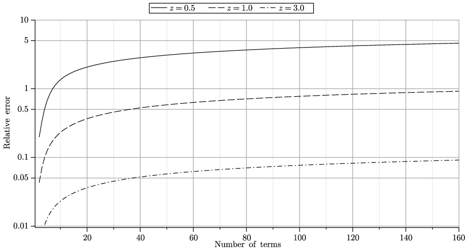
Numerical simulations show, however, that the greater nn, the greater the relative difference between the upper bound and the left–hand side in (67), see Fig. 3,
Refer to caption
Figure 3: Relative error between the upper bound and the left–hand side in (67) as a function of nn for three different values of argument zz, logarithmic scale.

and thus, this upper bound is relatively rough.3333 33 The error is mainly due to the use of inequality |ImΓ⁡(v)|⩽|Γ⁡(v)|\,|\mathop{\rm Im}\nolimits\Gamma(v)|\leqslant|\Gamma(v)|\,. A more accurate description of the behavior of sum (64) at large nn may be obtained by seeking its asymptotics. In order to find it, we proceed as follows. We first rewrite the second line of (65) as

i2​∫0∞{(−i​x2​π​z)n−(i​x2​π​z)n}​e−x​d​xx=∫0∞Im[(i​x2​π​z)n]​e−x​d​xx\frac{i}{2}\!\int\limits_{0}^{\infty}\!\left\{\!\left(-\frac{i\,x}{2\pi z}\right)_{\!n}-\left(\frac{i\,x}{2\pi z}\right)_{\!n}\!\right\}\frac{\,e^{-x}\,dx\,}{x}=\,\int\limits_{0}^{\infty}\!\mathop{\rm Im}\nolimits\left[\!\left(\frac{i\,x}{2\pi z}\right)_{\!n}\right]\frac{\,e^{-x}\,dx\,}{x} (68)

Now, it is well–known that function 1/Γ⁡(z)1/\Gamma(z) is regular on the entire complex zz–plane, and therefore, may be expanded into the MacLaurin’s series

1Γ⁡(z)=z+γ​z2+(γ22−π212)​z3+…≡∑k=1∞zk​ak,|z|<∞,\frac{1}{\Gamma(z)}\,=\,z+\gamma z^{2}+\left(\!\frac{\gamma^{2}}{2}-\frac{\pi^{2}}{12}\right)\!z^{3}+\ldots\,\equiv\sum_{k=1}^{\infty}z^{k}a_{k}\,,\qquad|z|<\infty\,, (69)

where

ak≡1k!⋅[1Γ⁡(z)]z=0(k)=(−1)kπ​k!⋅[sin⁡π​x⋅Γ⁡(x)]x=1(k)a_{k}\,\equiv\,\frac{1}{k!}\cdot\left[\frac{1}{\Gamma(z)}\right]^{(k)}_{z=0}\!=\,\frac{(-1)^{k}}{\,\pi\,k!\,}\cdot\Big[\sin\pi x\cdot\Gamma(x)\Big]^{(k)}_{x=1} (70)

the last representation for coefficients aka_{k}, which follows from the reflection formula for the Γ\Gamma--function, being often more suitable for computational purposes.3434 34 On the computation of aka_{k}, see also [1, p. 256, no 6.1.34], [161, pp. 344 & 349], [66]. Using approximation (13) for the Pochhammer symbol and the above MacLaurin series for 1/Γ⁡(z)1/\Gamma(z), we have for sufficiently large nn

Im[(i​x2​π​z)n]∼Im[ni​x2​π​z⋅Γ⁡(n)Γ⁡(i​x2​π​z)]=(n−1)!​Im[(cos⁡x​ln⁡n2​π​z+i​sin⁡x​ln⁡n2​π​z)⋅∑k=1∞ak⋅(i​x2​π​z)k]=(n−1)!​[cos⁡x​ln⁡n2​π​z⋅∑k=0∞(−1)k​a2​k+1​(x2​π​z)2​k+1+sin⁡x​ln⁡n2​π​z⋅∑k=1∞(−1)k​a2​k​(x2​π​z)2​k]\begin{array}[]{ll}\displaystyle\mathop{\rm Im}\nolimits\left[\!\left(\frac{i\,x}{2\pi z}\right)_{\!n}\right]\sim\,\mathop{\rm Im}\nolimits\left[\frac{n^{\frac{ix}{2\pi z}}\cdot\Gamma(n)}{\Gamma\left(\frac{ix}{2\pi z}\right)}\right]=\,(n-1)!\mathop{\rm Im}\nolimits\left[\!\left(\cos\frac{x\ln n}{2\pi z}+i\sin\frac{x\ln n}{2\pi z}\right)\!\cdot\!\sum_{k=1}^{\infty}a_{k}\cdot\!\left(\frac{i\,x}{2\pi z}\right)^{\!k}\right]\\[22.76219pt] \displaystyle\qquad\qquad=\,(n-1)!\left[\cos\frac{x\ln n}{2\pi z}\cdot\!\sum_{k=0}^{\infty}(-1)^{k}a_{2k+1}\left(\frac{x}{2\pi z}\right)^{\!2k+1}\!+\,\sin\frac{x\ln n}{2\pi z}\cdot\!\sum_{k=1}^{\infty}(-1)^{k}a_{2k}\left(\frac{x}{2\pi z}\right)^{\!2k}\right]\end{array} (71)

the error due to considering only the first term in (13) being negligible with respect to logarithmic terms which will appear later. Inserting this expression into (68), performing the term--by--term integration and taking into account that3535 35 These equalities are valid wherever the integrals on the left converge, see e.g. [29, p. 130], [97, p. 12], [85].

{∫0∞xs−1​e−z​x​cos⁡u​x​dx=Γ⁡(s)(z2+u2)s/2⋅cos⁡[s​arc​tg⁡uz]∫0∞xs−1​e−z​x​sin⁡u​x​dx=Γ⁡(s)(z2+u2)s/2⋅sin⁡[s​arc​tg⁡uz]\begin{cases}\displaystyle\int\limits_{0}^{\infty}\!x^{s-1}e^{-zx}\cos ux\,dx\,=\,\frac{\Gamma(s)}{\big(z^{2}+u^{2}\big)^{s/2}}\cdot\cos\left[s\mathop{\mathrm{arc\,tg}}\nolimits\frac{u}{z}\right]\\[17.07164pt] \displaystyle\int\limits_{0}^{\infty}\!x^{s-1}e^{-zx}\sin ux\,dx\,=\,\frac{\Gamma(s)}{\big(z^{2}+u^{2}\big)^{s/2}}\cdot\sin\left[s\mathop{\mathrm{arc\,tg}}\nolimits\frac{u}{z}\right]\end{cases} (72)

yields

∫0∞Im[(i​x2​π​z)n]​e−x​d​xx∼(n−1)!​∑k=0∞(−1)k​a2​k+1​(2​k)!(2​π​z)2​k+1⋅cos⁡[(2​k+1)​arc​tg⁡ln⁡n2​π​z][1+ln2⁡n4​π2​z2]k+12+(n−1)!∑k=1∞(−1)ka2​k(2​k−1)!(2​π​z)2​k⋅sin⁡[2​k​arc​tg⁡ln⁡n2​π​z][1+ln2⁡n4​π2​z2]k\begin{array}[]{ll}\displaystyle\int\limits_{0}^{\infty}\!\mathop{\rm Im}\nolimits\left[\!\left(\frac{i\,x}{2\pi z}\right)_{\!n}\right]\frac{\,e^{-x}\,dx\,}{x}\,\sim\,(n-1)!\sum_{k=0}^{\infty}(-1)^{k}a_{2k+1}\frac{(2k)!}{(2\pi z)^{2k+1}}\cdot\frac{\cos\left[(2k+1)\mathop{\mathrm{arc\,tg}}\nolimits\dfrac{\ln n}{2\pi z}\right]}{\left[1+\dfrac{\ln^{2}\!n}{4\pi^{2}z^{2}}\right]^{k+\frac{1}{2}}}\\[34.1433pt] \displaystyle\qquad\qquad\qquad\qquad\qquad\qquad\qquad+(n-1)!\sum_{k=1}^{\infty}(-1)^{k}a_{2k}\frac{(2k-1)!}{(2\pi z)^{2k}}\cdot\frac{\sin\left[2k\mathop{\mathrm{arc\,tg}}\nolimits\dfrac{\ln n}{2\pi z}\right]}{\left[1+\dfrac{\ln^{2}\!n}{4\pi^{2}z^{2}}\right]^{k}}\end{array}

Whence, the required asymptotics is

1n⋅n!​∑l=0⌊12​n⌋(−1)l​(2​l)!⋅|S1​(n,2​l+1)|(2​π​z)2​l+1==1n2​∑k=0∞(−1)k(2​k+1)​(4​π2​z2+ln2⁡n)k+12⋅cos⁡[(2​k+1)​arc​tg⁡ln⁡n2​π​z]⋅[1Γ⁡(x)]x=0(2​k+1)+1n2∑k=1∞(−1)k 2​k​(4​π2​z2+ln2⁡n)k⋅sin[2karc​tgln⁡n2​π​z]⋅[1Γ⁡(x)](2​k)x=0+O(1n3)\begin{array}[]{ll}\displaystyle\frac{1}{\,n\cdot n!\,}\!\!\sum_{l=0}^{\lfloor\frac{1}{2}n\rfloor}\!(-1)^{l}\frac{\,(2l)!\cdot|S_{1}(n,2l+1)|\,}{(2\pi z)^{2l+1}}\,=\\[17.07164pt] \displaystyle\qquad\qquad\quad=\frac{1}{\,n^{2}\,}\sum_{k=0}^{\infty}\frac{(-1)^{k}}{\,(2k+1)\big(4\pi^{2}z^{2}+\ln^{2}\!n\big)^{k+\frac{1}{2}}\,}\cdot\cos\left[(2k+1)\mathop{\mathrm{arc\,tg}}\nolimits\dfrac{\ln n}{2\pi z}\right]\cdot\left[\frac{1}{\Gamma(x)}\right]^{(2k+1)}_{x=0}\\[28.45274pt] \displaystyle\qquad\qquad\qquad\quad+\frac{1}{\,n^{2}\,}\sum_{k=1}^{\infty}\frac{(-1)^{k}}{\,2k\big(4\pi^{2}z^{2}+\ln^{2}\!n\big)^{k}\,}\cdot\sin\left[2k\mathop{\mathrm{arc\,tg}}\nolimits\dfrac{\ln n}{2\pi z}\right]\cdot\left[\frac{1}{\Gamma(x)}\right]^{(2k)}_{x=0}+O\!\left(\frac{1}{n^{3}}\right)\end{array} (73)

for sufficiently large nn. Retaining first few terms, we have

1n⋅n!​∑l=0⌊12​n⌋(−1)l​(2​l)!⋅|S1​(n,2​l+1)|(2​π​z)2​l+1= 2​π​zn2​{1 4​π2​z2+ln2⁡n−2​γ​ln⁡n(4​π2​z2+ln2⁡n)2}+O⁡(1n2​ln4​n),n→∞\begin{array}[]{ll}\displaystyle\frac{1}{\,n\cdot n!\,}\!\!\sum_{l=0}^{\lfloor\frac{1}{2}n\rfloor}\!(-1)^{l}\frac{\,(2l)!\cdot|S_{1}(n,2l+1)|\,}{(2\pi z)^{2l+1}}\,=\,\frac{\,2\pi z\,}{n^{2}}\left\{\frac{1}{\,4\pi^{2}z^{2}+\ln^{2}\!n\,}-\frac{2\gamma\ln n}{\,\big(4\pi^{2}z^{2}+\ln^{2}\!n\big)^{2}\,}\right\}\\[17.07164pt] \displaystyle\qquad\qquad\qquad\qquad\qquad\qquad\qquad\qquad\qquad+\,O\!\left(\frac{1}{n^{2}\ln^{4}\!n}\right)\,,\qquad n\to\infty\end{array} (74)

Thus, for moderate values of zz, series (63) converges approximately at the same rate as ∑(n​ln⁡n)−2\,\sum(n\ln n)^{-2}, i.e. at the same rate as, for example, Fontana–Mascheroni’s series (12), (47), see asymptotics (21).

III.1.3 Some important particular cases of the derived series

Refer to caption
Figure 4: Relative error of the series expansion for ln⁡Γ⁡(π−1)\ln\Gamma(\pi^{-1}) given by (75), logarithmic scale.

Let now consider some applications of the formula (63). In the first instance, it is natural to obtain a series expansion for

ln⁡Γ⁡(1π)=(1−1π)⋅ln⁡π−1π+12​ln⁡2+12​π​∑n=1∞1n⋅n!⋅{∑l=0⌊12​n⌋(−1)l​(2​l)!⋅|S1​(n,2​l+1)|22​l}=(1−1π)⋅ln⁡π−1π+12​ln⁡2+12​π​{1+14+112+132+175+1144+132880+15746 080+…}\begin{array}[]{ll}\displaystyle\ln\Gamma\!\left(\!\dfrac{1}{\,\pi\,}\!\right)&\displaystyle=\left(\!1-\frac{1}{\pi}\!\right)\!\cdot\ln\pi-\frac{1}{\pi}+\frac{1}{2}\ln 2+\frac{1}{2\pi}\!\sum_{n=1}^{\infty}\!\frac{1}{\,n\cdot n!\,}\cdot\Biggl\{\!\sum_{l=0}^{\lfloor\frac{1}{2}n\rfloor}\!(-1)^{l}\frac{(2l)!\cdot|S_{1}(n,2l+1)|}{2^{2l}}\Biggr\}\\[17.07164pt] &\displaystyle\!\!\!\!\!\!\!\!\!\!\!\!\!\!\!\!\!\!\!\!\!=\left(\!1-\frac{1}{\pi}\!\right)\!\cdot\ln\pi-\frac{1}{\pi}+\frac{1}{2}\ln 2+\frac{1}{2\pi}\left\{1+\frac{1}{4}+\frac{1}{12}+\frac{1}{32}+\frac{1}{75}+\frac{1}{144}+\frac{13}{2880}+\frac{157}{46\,080}+\ldots\right\}\end{array} (75)

The graphical illustration of the convergence of this series is given in Fig. 4. With equal ease, we derive

ln⁡Γ⁡(2π)=(1−2π)⋅ln⁡π−2π+2π​ln⁡2+14​π​∑n=1∞1n⋅n!⋅{∑l=0⌊12​n⌋(−1)l​(2​l)!⋅|S1​(n,2​l+1)|24​l}=(1−2π)⋅ln⁡π−2π+2π​ln⁡2+14​π​{1+14+548+7128+63119 200+1999216+19 5011 290 240+32 7072 949 120+…}\begin{array}[]{ll}\displaystyle\ln\Gamma\!\left(\!\dfrac{2}{\,\pi\,}\!\right)&\displaystyle=\left(\!1-\frac{2}{\pi}\!\right)\!\cdot\ln\pi-\frac{2}{\pi}+\frac{2}{\pi}\ln 2+\frac{1}{4\pi}\!\sum_{n=1}^{\infty}\!\frac{1}{\,n\cdot n!\,}\cdot\Biggl\{\!\sum_{l=0}^{\lfloor\frac{1}{2}n\rfloor}\!(-1)^{l}\frac{(2l)!\cdot|S_{1}(n,2l+1)|}{2^{4l}}\Biggr\}\\[17.07164pt] &\displaystyle\!\!\!\!\!\!\!\!\!\!\!\!\!\!\!\!\!\!\!\!\!\!\!\!\!\!\!\!\!\!=\left(\!1-\frac{2}{\pi}\!\right)\!\cdot\ln\pi-\frac{2}{\pi}+\frac{2}{\pi}\ln 2+\frac{1}{4\pi}\left\{1+\frac{1}{4}+\frac{5}{48}+\frac{7}{128}+\frac{631}{19\,200}+\frac{199}{9216}+\frac{19\,501}{1\,290\,240}+\frac{32\,707}{2\,949\,120}+\ldots\right\}\end{array} (76)

Many other similar expansions may be derived analogously. Let now see how the series behaves outside the region of convergence. For this aim, we take z=12​π−1z=\frac{1}{2}\pi^{-1}. Formula (63) yields

ln⁡Γ⁡(1 2​π)=?(1−12​π)⋅ln⁡2​π−12​π+1π​∑n=1∞1n⋅n!⋅{∑l=0⌊12​n⌋(−1)l​(2​l)!⋅|S1​(n,2​l+1)|}=(1−12​π)⋅ln⁡2​π−12​π+1π​{1+14−116−11300+1144+17630+1015760−311102 060−…}\begin{array}[]{ll}\displaystyle\ln\Gamma\!\left(\!\dfrac{1}{\,2\pi\,}\!\right)&\displaystyle\stackrel{{\scriptstyle?}}{{=}}\left(\!1-\frac{1}{2\pi}\!\right)\!\cdot\ln 2\pi-\frac{1}{2\pi}+\frac{1}{\pi}\sum_{n=1}^{\infty}\!\frac{1}{\,n\cdot n!\,}\cdot\Biggl\{\!\sum_{l=0}^{\lfloor\frac{1}{2}n\rfloor}\!(-1)^{l}(2l)!\cdot|S_{1}(n,2l+1)|\Biggr\}\\[17.07164pt] &\displaystyle=\left(\!1-\frac{1}{2\pi}\!\right)\!\cdot\ln 2\pi-\frac{1}{2\pi}+\frac{1}{\pi}\left\{1+\frac{1}{4}-\frac{1}{16}-\frac{11}{300}+\frac{1}{144}+\frac{17}{630}+\frac{101}{5760}-\frac{311}{102\,060}-\ldots\right\}\end{array} (77)

At first sight, it might seem that this alternating series slowly converges to ln⁡Γ⁡(12​π−1)≈1.765383194\ln\Gamma(\frac{1}{2}\pi^{-1})\approx 1.765383194: the summation of its first 3 terms gives the value 1.764207893​…1.764207893\ldots which corresponds to the relative accuracy ×10−46.6\!\times\!10^{-4}, that of 18 terms gives 1.765525087​…1.765525087\ldots, i.e. the relative accuracy ×10−58.0\!\times\!10^{-5}, the summation of first 32 terms yields 1.765392783​…1.765392783\ldots which corresponds to the relative error ×10−65.4\!\times\!10^{-6}.3636 36 We do not count the third term which is zero. Notwithstanding, further numerical simulations, see Fig. 5, leave no doubts: this series is divergent.

Refer to caption
Figure 5: Relative error of the series expansion for ln⁡Γ⁡(12​π−1)\ln\Gamma\big(\frac{1}{2}\pi^{-1}\big) given by (77), linear scale.

III.2 Second series expansion for the logarithm of the Γ\Gamma–function

Rewrite formula (63) for 2​z2z instead of zz, and subtract the result from (63). In virtue of Legendre’s duplication formula for the Γ\Gamma–function ln⁡Γ⁡(2​z)=(2​z−1)​ln⁡2−12​ln⁡π+ln⁡Γ⁡(z)+ln⁡Γ⁡(z+12)\ln\Gamma(2z)=(2z-1)\ln 2-\frac{1}{2}\ln\pi+\ln\Gamma(z)+\ln\Gamma(z+\frac{1}{2}), we have

ln⁡Γ⁡(12+z)=z​ln⁡z−z+1 2​ln⁡2​π−1π​∑n=1∞1n⋅n!​∑l=0⌊12​n⌋(−1)l​(2​l)!⋅(22​l+1−1)⋅|S1​(n,2​l+1)|(4​π​z)2​l+1=zlnz−z+1 2ln2π−1π{14​π​z+116​π​z+118(12​π​z−732​π3​z3)+396(12​π​z−716​π3​z3)+1600(6π​z−24532​π3​z3+93128​π5​z5)+14320(30π​z−157532​π3​z3+1395128​π5​z5)+…}\begin{array}[]{ll}\displaystyle\ln\Gamma\!\left(\frac{1}{2}+z\right)&\displaystyle=\,z\ln{z}-z+\frac{1}{\,2\,}\ln 2\pi-\frac{1}{\,\pi\,}\!\sum_{n=1}^{\infty}\!\frac{1}{\,n\cdot n!\,}\!\sum_{l=0}^{\lfloor\frac{1}{2}n\rfloor}\!(-1)^{l}\frac{\,(2l)!\cdot(2^{2l+1}-1)\cdot|S_{1}(n,2l+1)|\,}{(4\pi z)^{2l+1}}\\[14.22636pt] &\displaystyle\!\!\!\!\!\!\!\!\!\!\!\!\!\!=\,z\ln{z}-z+\frac{1}{\,2\,}\ln 2\pi-\frac{1}{\,\pi\,}\left\{\frac{1}{4\pi z}+\frac{1}{16\pi z}+\frac{1}{18}\left(\frac{1}{2\pi z}-\frac{7}{32\pi^{3}z^{3}}\right)+\frac{3}{96}\left(\frac{1}{2\pi z}-\frac{7}{16\pi^{3}z^{3}}\right)\right.\\[14.22636pt] &\displaystyle\!\!\!\!\!\!\!\!\!\!\!\!\!\!\quad\left.+\frac{1}{600}\left(\frac{6}{\pi z}-\frac{245}{32\pi^{3}z^{3}}+\frac{93}{128\pi^{5}z^{5}}\right)+\frac{1}{4320}\left(\frac{30}{\pi z}-\frac{1575}{32\pi^{3}z^{3}}+\frac{1395}{128\pi^{5}z^{5}}\right)+\ldots\right\}\end{array} (78)

which holds in the green zone shown in Fig. 2. This expression allows to expand any value of the form ln⁡Γ⁡(12+α​π−1)\ln\Gamma(\frac{1}{2}+\alpha\pi^{-1}) into the series with rational coefficients if α\alpha is rational greater than 16​π\frac{1}{6}\pi. For example, putting z=π−1z=\pi^{-1}, we have

ln⁡Γ⁡(12+1π)\displaystyle\displaystyle\ln\Gamma\!\left(\!\dfrac{1}{2}+\dfrac{1}{\,\pi\,}\!\right)\; =−1+ln⁡ππ+1 2​ln⁡2​π−1 4​π​∑n=1∞1n⋅n!​∑l=0⌊12​n⌋(−1)l​(2​l)!⋅(22​l+1−1)⋅|S1​(n,2​l+1)|24​l\displaystyle\displaystyle=\,-\frac{1+\ln\pi}{\pi}+\frac{1}{\,2\,}\ln 2\pi-\frac{1}{\,4\pi\,}\!\sum_{n=1}^{\infty}\!\frac{1}{\,n\cdot n!\,}\!\sum_{l=0}^{\lfloor\frac{1}{2}n\rfloor}\!(-1)^{l}\frac{\,(2l)!\cdot(2^{2l+1}-1)\cdot|S_{1}(n,2l+1)|\,}{2^{4l}}
=−1+ln⁡ππ+1 2​ln⁡2​π−1 4​π​{1+14+116+1128−11919 200−719216−78531 290 240−12 6112 949 120−…}\displaystyle\displaystyle\!\!\!\!\!\!\!\!\!\!\!\!\!\!\!\!\!\!\!\!\!\!\!\!\!\!=\,-\frac{1+\ln\pi}{\pi}+\frac{1}{\,2\,}\ln 2\pi-\frac{1}{\,4\pi\,}\!\left\{1+\frac{1}{4}+\frac{1}{16}+\frac{1}{128}-\frac{119}{19\,200}-\frac{71}{9216}-\frac{7853}{1\,290\,240}-\frac{12\,611}{2\,949\,120}-\ldots\right\}

Furthermore, both series expansions (63) and (78), used together with the reflection formula and the recurrence relationship for the Γ\Gamma–function, yield series with rational coefficients for any values of the form ln⁡Γ⁡(12​n±α​π−1)\ln\Gamma(\frac{1}{2}n\pm\alpha\pi^{-1}), where nn is integer.

As a final remark, we note that expression (78), written for zz instead of 12+z\frac{1}{2}+z, straightforwardly produces another series expansion for the logarithm of the Γ\Gamma–function

ln⁡Γ⁡(z)=\displaystyle\displaystyle\ln\Gamma(z)= (z−1 2)​ln⁡(z−1 2)−z+1 2+1 2​ln⁡2​π\displaystyle\displaystyle\left(z-\frac{1}{\,2\,}\right)\!\ln\!{\left(z-\frac{1}{\,2\,}\right)}-z+\frac{1}{\,2\,}+\frac{1}{\,2\,}\ln 2\pi (79)
−1π∑n=1∞1n⋅n!∑l=0⌊12​n⌋(−1)l(2​l)!⋅(22​l+1−1)⋅|S1​(n,2​l+1)|(4​π)2​l+1⋅(z−12)2​l+1\displaystyle\displaystyle-\frac{1}{\,\pi\,}\!\sum_{n=1}^{\infty}\!\frac{1}{\,n\cdot n!\,}\!\sum_{l=0}^{\lfloor\frac{1}{2}n\rfloor}\!(-1)^{l}\frac{\,(2l)!\cdot(2^{2l+1}-1)\cdot|S_{1}(n,2l+1)|\,}{(4\pi)^{2l+1}\cdot\big(z-\frac{1}{2}\big)^{2l+1}}

which converges in the green zone given in Fig. 2 shifted by 12\frac{1}{2} to the right. In particular, if zz is real, it converges for any z>23z>\frac{2}{3}.

Remark Expansion (78) may be also derived if we replace in (58) Binet’s formula by its analog with “conjugated” denominator

∫0∞arc​tg⁡a​xeb​x+1​𝑑x=−πb​ln⁡Γ⁡(12+b 2​π​a)−1 2​a​(1+ln⁡2​π​ab)+π 2​b​ln​2​π.\int\limits_{0}^{\,\infty}\!\frac{\,\mathop{\mathrm{arc\,tg}}\nolimits{ax}\,}{e^{bx}+1}\,dx\,=\,-\frac{\,\pi\,}{b}\ln\Gamma\!\left(\!\dfrac{1}{2}+\dfrac{b}{\,2\pi a\,}\!\right)-\frac{1}{\,2a\,}\!\left(1+\ln\frac{2\pi a}{b}\right)+\frac{\,\pi\,}{\,2b\,}\ln 2\pi.

where a>0a>0 and Reb>0\mathop{\rm Re}\nolimits{b}>0, see [13, Sect. 4, exercise no 40-a], or if we replace it by the following formula

∫0∞arc​tg⁡a​xshb​x​𝑑x=πb​{ln⁡Γ⁡(b 2​π​a)−ln⁡Γ⁡(12+b 2​π​a)−12​ln​2​π​ab}\int\limits_{0}^{\,\infty}\!\frac{\,\mathop{\mathrm{arc\,tg}}\nolimits{ax}\,}{\mathop{\rm sh}\nolimits{bx}}\,dx\,=\,\frac{\,\pi\,}{b}\left\{\ln\Gamma\!\left(\!\dfrac{b}{\,2\pi a\,}\!\right)-\ln\Gamma\!\left(\!\dfrac{1}{2}+\dfrac{b}{\,2\pi a\,}\!\right)-\frac{1}{2}\ln\frac{2\pi a}{b}\right\}

derived in [13, Sect. 4, exercise no 39-e]. Making a change of variable x=−2barcthu\,x=-\frac{2}{b}\mathop{\rm arcth}\nolimits u\,, and then, proceeding analogously to (59)–(63), yields

ln⁡Γ⁡(z)−ln⁡Γ⁡(12+z)=−12​ln​z+1π​∑n=0∞1 2​n+1​∑k=12​n+12kk!​(2​nk−1)​∑l=0n(−1)l​(2​l)!⋅S1​(k,2​l+1)(2​π​z)2​l+1\begin{array}[]{l}\displaystyle\ln\Gamma(z)-\ln\Gamma\!\left(\frac{1}{2}+z\right)=\,-\frac{1}{2}\ln{z}+\frac{1}{\pi}\sum_{n=0}^{\infty}\frac{1}{\,2n+1\,}\!\sum_{k=1}^{2n+1}\frac{2^{k}}{k!}\binom{2n}{k-1}\sum_{l=0}^{n}(-1)^{l}\frac{(2l)!\cdot S_{1}(k,2l+1)}{(2\pi z)^{2l+1}}\end{array} (80)

which, being combined with (78), leads to a rearranged version of (63).

III.3 Series expansion for the polygamma functions

By differentiating expressions (63) and (79), one may easily deduce similar series expansions for the polygamma functions. Differentiating the former expansion yields the following series representations for the digamma and trigamma functions

Ψ⁡(z)=ln⁡z−1 2​z−1π​z​∑n=1∞1n⋅n!​∑l=0⌊12​n⌋(−1)l​(2​l+1)!⋅|S1​(n,2​l+1)|(2​π​z)2​l+1=lnz−1 2​z−1π​z{12​π​z+18​π​z+118(1π​z−34​π3​z3)+396(1π​z−32​π3​z3)+1600(12π​z−1054​π3​z3+154​π5​z5)+14320(60π​z−6754​π3​z3+2254​π5​z5)+…}\begin{array}[]{ll}\displaystyle\Psi(z)&\displaystyle=\,\ln z-\frac{1}{\,2z\,}-\frac{1}{\,\pi z\,}\!\sum_{n=1}^{\infty}\!\frac{1}{\,n\cdot n!\,}\!\sum_{l=0}^{\lfloor\frac{1}{2}n\rfloor}\!(-1)^{l}\frac{\,(2l+1)!\cdot|S_{1}(n,2l+1)|\,}{(2\pi z)^{2l+1}}\\[14.22636pt] &\displaystyle=\,\ln z-\frac{1}{\,2z\,}-\frac{1}{\,\pi z\,}\left\{\frac{1}{2\pi z}+\frac{1}{8\pi z}+\frac{1}{18}\left(\frac{1}{\pi z}-\frac{3}{4\pi^{3}z^{3}}\right)+\frac{3}{96}\left(\frac{1}{\pi z}-\frac{3}{2\pi^{3}z^{3}}\right)\right.\\[14.22636pt] &\displaystyle\quad\left.+\frac{1}{600}\left(\frac{12}{\pi z}-\frac{105}{4\pi^{3}z^{3}}+\frac{15}{4\pi^{5}z^{5}}\right)+\frac{1}{4320}\left(\frac{60}{\pi z}-\frac{675}{4\pi^{3}z^{3}}+\frac{225}{4\pi^{5}z^{5}}\right)+\ldots\right\}\end{array} (81)

and

Ψ1​(z)=1 2​z2+1z+1π​z2​∑n=1∞1n⋅n!​∑l=0⌊12​n⌋(−1)l​(2​l+2)!⋅|S1​(n,2​l+1)|(2​π​z)2​l+1=1 2​z2+1z+1π​z2{1π​z+14​π​z+118(2π​z−3π3​z3)+396(2π​z−6π3​z3)+1600(24π​z−105π3​z3+452​π5​z5)+14320(120π​z−675π3​z3+6752​π5​z5)+…}\begin{array}[]{ll}\displaystyle\Psi_{1}(z)&\displaystyle=\,\frac{1}{\,2z^{2}\,}+\frac{1}{\,z\,}+\frac{1}{\,\pi z^{2}\,}\!\sum_{n=1}^{\infty}\!\frac{1}{\,n\cdot n!\,}\!\sum_{l=0}^{\lfloor\frac{1}{2}n\rfloor}\!(-1)^{l}\frac{\,(2l+2)!\cdot|S_{1}(n,2l+1)|\,}{(2\pi z)^{2l+1}}\\[14.22636pt] &\displaystyle=\,\frac{1}{\,2z^{2}\,}+\frac{1}{\,z\,}+\frac{1}{\,\pi z^{2}\,}\left\{\frac{1}{\pi z}+\frac{1}{4\pi z}+\frac{1}{18}\left(\frac{2}{\pi z}-\frac{3}{\pi^{3}z^{3}}\right)+\frac{3}{96}\left(\frac{2}{\pi z}-\frac{6}{\pi^{3}z^{3}}\right)\right.\\[14.22636pt] &\displaystyle\quad\left.+\frac{1}{600}\left(\frac{24}{\pi z}-\frac{105}{\pi^{3}z^{3}}+\frac{45}{2\pi^{5}z^{5}}\right)+\frac{1}{4320}\left(\frac{120}{\pi z}-\frac{675}{\pi^{3}z^{3}}+\frac{675}{2\pi^{5}z^{5}}\right)+\ldots\right\}\end{array} (82)

respectively. More generally, by differentiating kk times with respect to zz the above series for Ψ⁡(z)\Psi(z), we obtain a series expansion for the kkth polygamma function

Ψk​(z)=(−1)k+1​k! 2​zk+1+(−1)k+1​(k−1)!zk+(−1)k+1π​zk+1​∑n=1∞1n⋅n!​∑l=0⌊12​n⌋(−1)l​(2​l+k+1)!⋅|S1​(n,2​l+1)|(2​π​z)2​l+1=(−1)k+1k! 2​zk+1+(−1)k+1(k−1)!zk+(−1)k+1π​zk+1{(k+1)!2​π​z+(k+1)!8​π​z+118[(k+1)!π​z−(k+3)!8​π3​z3]+396[(k+1)!π​z−(k+3)!4​π3​z3]+1600[12​(k+1)!π​z−35​(k+3)!8​π3​z3+(k+5)!32​π5​z5]+…}\begin{array}[]{ll}\displaystyle\Psi_{k}(z)&\displaystyle=\,(-1)^{k+1}\frac{k!}{\,2z^{k+1}\,}+(-1)^{k+1}\frac{(k-1)!}{\,z^{k}\,}+\frac{(-1)^{k+1}}{\,\pi z^{k+1}\,}\!\sum_{n=1}^{\infty}\!\frac{1}{\,n\cdot n!\,}\!\sum_{l=0}^{\lfloor\frac{1}{2}n\rfloor}\!(-1)^{l}\frac{\,(2l+k+1)!\cdot|S_{1}(n,2l+1)|\,}{(2\pi z)^{2l+1}}\\[14.22636pt] &\displaystyle=\,(-1)^{k+1}\frac{k!}{\,2z^{k+1}\,}+(-1)^{k+1}\frac{(k-1)!}{\,z^{k}\,}+\frac{(-1)^{k+1}}{\,\pi z^{k+1}\,}\!\left\{\frac{(k+1)!}{2\pi z}+\frac{(k+1)!}{8\pi z}+\frac{1}{18}\left[\frac{(k+1)!}{\pi z}-\frac{(k+3)!}{8\pi^{3}z^{3}}\right]\right.\\[14.22636pt] &\displaystyle\quad\left.+\frac{3}{96}\left[\frac{(k+1)!}{\pi z}-\frac{(k+3)!}{4\pi^{3}z^{3}}\right]+\frac{1}{600}\left[\frac{12\,(k+1)!}{\pi z}-\frac{35\,(k+3)!}{8\pi^{3}z^{3}}+\frac{(k+5)!}{32\pi^{5}z^{5}}\right]+\ldots\right\}\end{array} (83)

where k=1,2,3,…k=1,2,3,\ldots Convergence analysis of these series is analogous to that performed in Section III.1.2, and we omit the details because the calculations are a little bit long. This analysis reveals that the general term of these series may be always bounded by αk​(z)​n−2\alpha_{k}(z)n^{-2}, where αk​(z)\alpha_{k}(z) depends solely on zz and on the order of the polygamma function kk. At large nn, the general term of these series is of the same order as (n​lnm​n)−2\big(n\ln^{m}\!n\big)^{-2}, where m=1m=1 for Ψ⁡(z)\Psi(z), m=2m=2 for Ψ1​(z)\Psi_{1}(z) and Ψ2​(z)\Psi_{2}(z), m=3m=3 for Ψ3​(z)\Psi_{3}(z) and Ψ4​(z)\Psi_{4}(z), and so on.

We now give several particular cases of the above expansions. From (81)–(83), it follows that at π−1\pi^{-1}, the polygamma functions have the following series representations

Ψ⁡(1π)=−ln⁡π−π 2−∑n=1∞1n⋅n!​∑l=0⌊12​n⌋(−1)l​(2​l+1)!⋅|S1​(n,2​l+1)|22​l+1=−ln⁡π−π 2−12−18−172+164+7400+7576+64394 080+10330 720+…\begin{array}[]{ll}\displaystyle\Psi\!\left(\!\dfrac{1}{\,\pi\,}\!\right)&\displaystyle=\,-\ln\pi-\frac{\pi}{\,2\,}-\sum_{n=1}^{\infty}\!\frac{1}{\,n\cdot n!\,}\!\sum_{l=0}^{\lfloor\frac{1}{2}n\rfloor}\!(-1)^{l}\frac{\,(2l+1)!\cdot|S_{1}(n,2l+1)|\,}{2^{2l+1}}\\[17.07164pt] &\displaystyle=-\ln\pi-\frac{\pi}{\,2\,}-\frac{1}{2}-\frac{1}{8}-\frac{1}{72}+\frac{1}{64}+\frac{7}{400}+\frac{7}{576}+\frac{643}{94\,080}+\frac{103}{30\,720}+\ldots\end{array} (84)
Ψ1​(1π)=π2 2+π+π​∑n=1∞1n⋅n!​∑l=0⌊12​n⌋(−1)l​(2​l+2)!⋅|S1​(n,2​l+1)|22​l+1=π2 2+π+π⁡{1+14−118−18−39400−29576−35323 520+113840+…}\begin{array}[]{ll}\displaystyle\Psi_{1}\!\left(\!\dfrac{1}{\,\pi\,}\!\right)&\displaystyle=\,\frac{\pi^{2}}{\,2\,}+\pi+\pi\!\sum_{n=1}^{\infty}\!\frac{1}{\,n\cdot n!\,}\!\sum_{l=0}^{\lfloor\frac{1}{2}n\rfloor}\!(-1)^{l}\frac{\,(2l+2)!\cdot|S_{1}(n,2l+1)|\,}{2^{2l+1}}\\[17.07164pt] &\displaystyle=\,\frac{\pi^{2}}{\,2\,}+\pi+\pi\left\{1+\frac{1}{4}-\frac{1}{18}-\frac{1}{8}-\frac{39}{400}-\frac{29}{576}-\frac{353}{23\,520}+\frac{11}{3840}+\ldots\right\}\end{array} (85)

and, more generally, for k=1,2,3,…k=1,2,3,\ldots\,

Ψk​(1π)=(−1)k+1​πk⋅{π​k! 2+(k−1)!+∑n=1∞1n⋅n!​∑l=0⌊12​n⌋(−1)l​(2​l+k+1)!⋅|S1​(n,2​l+1)|22​l+1}=(−1)k+1πk⋅{π​k! 2+(k−1)!+(1+k)!2+(1+k)!8+118[(k+1)!−(k+3)!8]+396[(k+1)!−(k+3)!4]+1600[12(k+1)!−35​(k+3)!8+(k+5)!32]+…}\begin{array}[]{ll}\displaystyle\Psi_{k}\!\left(\!\dfrac{1}{\,\pi\,}\!\right)&\displaystyle=\,(-1)^{k+1}\pi^{k}\cdot\left\{\frac{\pi\,k!}{\,2\,}+(k-1)!+\sum_{n=1}^{\infty}\!\frac{1}{\,n\cdot n!\,}\!\sum_{l=0}^{\lfloor\frac{1}{2}n\rfloor}\!(-1)^{l}\frac{\,(2l+k+1)!\cdot|S_{1}(n,2l+1)|\,}{2^{2l+1}}\right\}\\[17.07164pt] &\displaystyle=\,(-1)^{k+1}\pi^{k}\cdot\left\{\frac{\pi\,k!}{\,2\,}+(k-1)!+\frac{(1+k)!}{2}+\frac{(1+k)!}{8}+\frac{1}{18}\left[(k+1)!-\frac{(k+3)!}{8}\right]\right.\\[17.07164pt] &\displaystyle\quad\left.+\frac{3}{96}\left[(k+1)!-\frac{(k+3)!}{4}\right]+\frac{1}{600}\left[12\,(k+1)!-\frac{35\,(k+3)!}{8}+\frac{(k+5)!}{32}\right]+\ldots\right\}\end{array} (86)

Figure 6 shows the rate of convergence of first two series.

Refer to caption
Refer to caption
Figure 6: Top: Relative error of the series expansion for Ψ⁡(π−1)\,\Psi(\pi^{-1})\, given by (84). Bottom: Relative error of the series expansion for Ψ1​(π−1)\,\Psi_{1}(\pi^{-1})\, given by (86). For better visibility, both errors are presented in absolute values and logarithmic scales.

Second variant of the series expansions for the polygamma functions follows from (79). Differentiating the latter with respect to zz yields

Ψ⁡(z)=ln⁡(z−1 2)+1π​∑n=1∞1n⋅n!​∑l=0⌊12​n⌋(−1)l​(2​l+1)!⋅(22​l+1−1)⋅|S1​(n,2​l+1)|(4​π)2​l+1⋅(z−12)2​l+2\Psi(z)\,=\,\ln\!{\left(z-\frac{1}{\,2\,}\right)}+\frac{1}{\,\pi\,}\!\sum_{n=1}^{\infty}\!\frac{1}{\,n\cdot n!\,}\!\sum_{l=0}^{\lfloor\frac{1}{2}n\rfloor}\!(-1)^{l}\frac{\,(2l+1)!\cdot(2^{2l+1}-1)\cdot|S_{1}(n,2l+1)|\,}{(4\pi)^{2l+1}\cdot\big(z-\frac{1}{2}\big)^{2l+2}}\vskip-4.2679pt (87)

and

Ψk​(z)=(−1)k+1​(k−1)!(z−12)k+(−1)kπ​∑n=1∞1n⋅n!​∑l=0⌊12​n⌋(−1)l​(2​l+k+1)!⋅(22​l+1−1)⋅|S1​(n,2​l+1)|(4​π)2​l+1⋅(z−12)2​l+k+2\Psi_{k}(z)\,=\,\frac{\,(-1)^{k+1}(k-1)!\,}{\big(z-\frac{1}{2}\big)^{k}}+\frac{(-1)^{k}}{\,\pi\,}\!\sum_{n=1}^{\infty}\!\frac{1}{\,n\cdot n!\,}\!\sum_{l=0}^{\lfloor\frac{1}{2}n\rfloor}\!(-1)^{l}\frac{\,(2l+k+1)!\cdot(2^{2l+1}-1)\cdot|S_{1}(n,2l+1)|\,}{(4\pi)^{2l+1}\cdot\big(z-\frac{1}{2}\big)^{2l+k+2}} (88)

In particular,

Ψ⁡(1 2+1π)=−ln⁡π+∑n=1∞1n⋅n!​∑l=0⌊12​n⌋(−1)l​(2​l+1)!⋅(22​l+1−1)⋅|S1​(n,2​l+1)|24​l+2=−ln⁡π+14+116−5576−13512−56925 600−53936 864−98 67112 042 240−…\begin{array}[]{ll}\displaystyle\Psi\!\left(\!\dfrac{1}{\,2\,}+\dfrac{1}{\,\pi\,}\!\right)&\displaystyle=\,-\ln\pi+\sum_{n=1}^{\infty}\!\frac{1}{\,n\cdot n!\,}\!\sum_{l=0}^{\lfloor\frac{1}{2}n\rfloor}\!(-1)^{l}\frac{\,(2l+1)!\cdot(2^{2l+1}-1)\cdot|S_{1}(n,2l+1)|\,}{2^{4l+2}}\\[17.07164pt] &\displaystyle=-\ln\pi+\frac{1}{4}+\frac{1}{16}-\frac{5}{576}-\frac{13}{512}-\frac{569}{25\,600}-\frac{539}{36\,864}-\frac{98\,671}{12\,042\,240}-\ldots\end{array} (89)

Similarly to expansions for ln⁡Γ⁡(z)\ln\Gamma(z), expansions (83) and (88), combined with the reflection formula and the recurrence relationship for polygamma functions, give series with rational coefficients for any polygamma function of the argument 12​n±α​π−1\,\frac{1}{2}n\pm\alpha\pi^{-1}\,, where α\alpha is rational greater than 16​π\frac{1}{6}\pi and nn is integer.

Final remark Series which we discovered in the present work are very interesting especially because of the implication of combinatorial numbers S1​(n,l)S_{1}(n,l). In this context, it seems appropriate to note that series of a similar nature for ln⁡Γ⁡(z)\ln\Gamma(z) and Ψk​(z)\Psi_{k}(z) were already obtained, but remain little–known and practically not mentioned in modern literature. For instance, in 1839, Jacques Binet [12, pp. 231–236, 257, 237, 235, 335–339, Eqs. (63), (81)] obtained several, rapidly convergent for large |z||z|, expansions

ln⁡Γ⁡(z)=(z−1 2)​ln⁡z−z+1 2​ln⁡2​π+12​∑n=1∞I⁡(n)n⋅1(z+1)nln⁡Γ⁡(z)=(z−1 2)​ln⁡z−z+1 2​ln⁡2​π−12​∑n=1∞I′​(n)n⋅1(z)nΨ⁡(z)=ln⁡z−12​z−12​∑n=2∞K⁡(n)n⋅1(z+1)nΨ⁡(z)=ln⁡z−12​z−12​∑n=2∞K⁡(n)−n​K​(n−1)n⋅1(z)n\begin{array}[]{l}\displaystyle\ln\Gamma(z)\,=\,\left(z-\frac{1}{\,2\,}\right)\!\ln z-z+\frac{1}{\,2\,}\ln 2\pi+\frac{1}{2}\!\sum_{n=1}^{\infty}\frac{I(n)}{n}\cdot\frac{1}{(z+1)_{n}}\\[14.22636pt] \displaystyle\ln\Gamma(z)\,=\,\left(z-\frac{1}{\,2\,}\right)\!\ln z-z+\frac{1}{\,2\,}\ln 2\pi-\frac{1}{2}\!\sum_{n=1}^{\infty}\frac{I^{\prime}(n)}{n}\cdot\frac{1}{(z)_{n}}\\[14.22636pt] \displaystyle\Psi(z)\,=\,\ln z-\frac{1}{2z}-\frac{1}{2}\!\sum_{n=2}^{\infty}\!\frac{K(n)}{n}\cdot\frac{1}{(z+1)_{n}}\\[14.22636pt] \displaystyle\Psi(z)\,=\,\ln z-\frac{1}{2z}-\frac{1}{2}\!\sum_{n=2}^{\infty}\!\frac{K(n)-nK(n-1)}{n}\cdot\frac{1}{(z)_{n}}\end{array} (90)

where numbers I⁡(n)I(n), I′​(n)I^{\prime}(n) and K⁡(n)K(n) are rational and may be given in terms of the Stirling numbers of the first kind. Binet recognized these numbers, denoted them by a capital HH, referenced Stirling’s treatise [146] and even corrected Striling’s error: in the table on p. 11 [146] he noticed that the value of |S1​(9,3)|=118 124|S_{1}(9,3)|=118\,124 and not 105 056105\,056. In our notations, Binet’s formulæ for I⁡(n)I(n), I′​(n)I^{\prime}(n) and K⁡(n)K(n) read

I⁡(n)=∫01(2​x−1)​(x)n​𝑑x=∑l=1nl⋅|S1​(n,l)|(l+1)​(l+2)=∑l=1n|S1​(n,l)|l+2−C2,nI′​(n)=∫01(2​x−1)​(1−x)​(x)n−1​𝑑x=∑l=1n−2l⋅|S1​(n−1,l+1)|(l+2)​(l+3)​(l+4)K⁡(n)=n!−∫01(x)n​𝑑x=n!−∑l=1n|S1​(n,l)|l+1=n!−2​C2,n\begin{array}[]{l}\displaystyle I(n)\,=\int\limits_{0}^{1}\!(2x-1)(x)_{n}\,dx=\sum_{l=1}^{n}\frac{l\cdot\big|S_{1}(n,l)\big|}{(l+1)(l+2)}\,=\,2\!\sum_{l=1}^{n}\frac{\big|S_{1}(n,l)\big|}{\,l+2\,}\,-\ \,C_{2,n}\\[14.22636pt] \displaystyle I^{\prime}(n)\,=\int\limits_{0}^{1}\!(2x-1)(1-x)(x)_{n-1}\,dx=\sum_{l=1}^{n-2}\frac{l\cdot\big|S_{1}(n-1,l+1)\big|}{(l+2)(l+3)(l+4)}\\[14.22636pt] \displaystyle K(n)\,=\,n!-2\!\int\limits_{0}^{1}\!(x)_{n}\,dx=\,n!-2\!\sum_{l=1}^{n}\frac{\big|S_{1}(n,l)\big|}{\,l+1\,}\,=\,n!-2C_{2,n}\end{array} (91)

In particular, the first few coefficients are I⁡(1)=16I(1)=\frac{1}{6}, I⁡(2)=13I(2)=\frac{1}{3}, I⁡(3)=5960I(3)=\frac{59}{60}, I⁡(4)=5815I(4)=\frac{58}{15}, I⁡(5)=53328I(5)=\frac{533}{28}, I⁡(6)=157714I(6)=\frac{1577}{14}, … , I′​(1)=−16I^{\prime}(1)=-\frac{1}{6}, I′​(2)=0I^{\prime}(2)=0, I′​(3)=+160I^{\prime}(3)=+\frac{1}{60}, I′​(4)=+115I^{\prime}(4)=+\frac{1}{15}, I′​(5)=+2584I^{\prime}(5)=+\frac{25}{84}, I′​(6)=+117I^{\prime}(6)=+\frac{11}{7}, …  and K⁡(2)=13K(2)=\frac{1}{3}, K⁡(3)=32K(3)=\frac{3}{2}, K⁡(4)=10915K(4)=\frac{109}{15}, K⁡(5)=2456K(5)=\frac{245}{6}, K⁡(6)=11 15342K(6)=\frac{11\,153}{42}, K⁡(7)=23 68112K(7)=\frac{23\,681}{12}, …3737 37 Values I′​(1)=−16I^{\prime}(1)=-\frac{1}{6}, I′​(2)=0I^{\prime}(2)=0 are found from the integral formula, their definition via the sum with the Stirling numbers of the first kind being valid only for n⩾3n\geqslant 3. Strictly speaking, Binet only found first four coefficients for each of these series and incorrectly calculated some of them (e.g. for I⁡(4)I(4) he took 22760\frac{227}{60} instead of 23260=5815\frac{232}{60}=\frac{58}{15}, for K⁡(5)K(5) he took 2453\frac{245}{3} instead of 2456\frac{245}{6}), but otherwise his method and derivations are correct. Binet also remarked that

I′​(n)n⋅1(z)n=O⁡(1nz+1​ln⁡n),n→∞,\frac{I^{\prime}(n)}{n}\cdot\frac{1}{(z)_{n}}\,=\,O\left(\frac{1}{n^{z+1}\ln n}\right)\,,\qquad n\to\infty\,, (92)

which implies that he knew the first--order approximation for the Cauchy numbers of the second kind as early as 1839.3838 38 Note, however, that Binet stated this result without proof (he wrote Je ne développe pas ici ces résultats, parce que les détails sont un peu longs). In 1923 Niels E. Nørlund [112, pp. 243–244], [151, p. 335] obtained two series of a similar nature for the polygamma functions. In particular, for the Digamma function, he provided following expressions

Ψ⁡(z)=ln⁡z−1z+∑n=1∞C2,nn⋅1(z+1)nΨ⁡(z)=ln⁡z−12​z−∑n=2∞|Gn|⋅(n−1)!(z)n\begin{array}[]{l}\displaystyle\Psi(z)\,=\,\ln z-\frac{1}{z}+\!\sum_{n=1}^{\infty}\frac{C_{2,n}}{n}\cdot\frac{1}{(z+1)_{n}}\\[14.22636pt] \displaystyle\Psi(z)\,=\,\ln z-\frac{1}{2z}-\!\sum_{n=2}^{\infty}\frac{\big|G_{n}\big|\cdot(n-1)!}{(z)_{n}}\end{array} (93)

A careful inspection of both formulæ reveals that they actually are rewritten versions of the foregoing expansions for Ψ⁡(z)\Psi(z) given by Binet 84 years earlier.3939 39 In order to reduce first Binet’s series to first Nørlund’s series, it suffices to remark that ∑n=2∞(n−1)!(z+1)n=∑n=1∞1⋅2⋯n(z+1)(z+2)⋯(z+n+1)=1z−1z+1\sum\limits_{n=2}^{\infty}\!\frac{(n-1)!}{(z+1)_{n}}=\sum\limits_{n=1}^{\infty}\!\frac{1\cdot 2\cdots n}{(z+1)(z+2)\cdots(z+n+1)}=\frac{1}{\,z\,}-\frac{1}{\,z+1\,} and C2,1=12C_{2,1}=\frac{1}{2}. The equivalence between second Binet’s series and second Nørlund’s series follows from the fact that 12​[K⁡(n)−n​K​(n−1)]=n​C2,n−1−C2,n=|C1,n|≡|Gn|⋅n!\frac{1}{2}\big[K(n)-nK(n-1)\big]=nC_{2,n-1}-C_{2,n}=\big|C_{1,n}\big|\equiv\big|G_{n}\big|\cdot n!\,, where K⁡(1)=0K(1)=0 and n=2,3,4,…n=2,3,4,\ldots One may also notice that Fontana–Masceroni series (12), (47), is a particular case of the latter formula when z=1z=1. In contrast, the former expression at z=1z=1 yields a not particularly well–known series for Euler’s constant

γ= 1−∑n=1∞C2,nn⋅(n+1)!= 1−14−572−132−25114 400−191728−19 0872 540 160−…\gamma\,=\,1-\sum_{n=1}^{\infty}\!\frac{C_{2,n}}{\,n\cdot(n+1)!\,}=\,1-\frac{1}{4}-\frac{5}{72}-\frac{1}{32}-\frac{251}{14\,400}-\frac{19}{1728}-\frac{19\,087}{2\,540\,160}-\ldots (94)

which is, in fact, closely related to the above–mentioned Fontana–Masceroni series and may be reduced to the latter by means of the recurrence relation

nC2,n−1−C2,n=|C1,n|≡|Gn|⋅n!,C2,0=1,n=1,2,3,…nC_{2,n-1}-C_{2,n}=\big|C_{1,n}\big|\equiv\big|G_{n}\big|\cdot n!\,,\qquad C_{2,0}=1\,,\quad n=1,2,3,\ldots (95)

Namely, by partial fraction decomposition, (94) becomes

γ= 1−∑n=1∞C2,nn!⋅1n⁡(n+1)= 1−∑n=1∞C2,nn⋅n!+∑n=1∞C2,n(n+1)!== 1−∑n=1∞C2,n−1−|Gn|⋅(n−1)!n!+∑n=1∞C2,n(n+1)!=∑n=1∞|Gn|n\begin{array}[]{l}\displaystyle\gamma\,=\,1-\sum_{n=1}^{\infty}\!\frac{C_{2,n}}{\,n!\,}\cdot\frac{1}{\,n(n+1)\,}\,=\,1-\sum_{n=1}^{\infty}\!\frac{C_{2,n}}{\,n\cdot n!\,}+\sum_{n=1}^{\infty}\!\frac{C_{2,n}}{\,(n+1)!\,}\,=\\[17.07164pt] \displaystyle\phantom{\gamma\,}=\,1-\sum_{n=1}^{\infty}\!\frac{C_{2,n-1}-\big|G_{n}\big|\cdot(n-1)!}{\,n!\,}+\sum_{n=1}^{\infty}\!\frac{C_{2,n}}{\,(n+1)!\,}\,=\sum_{n=1}^{\infty}\!\frac{\,\big|G_{n}\big|\,}{\,n\,}\end{array}

It is interesting to note that series (94) converges at the same rate as ∑n−2​ln−1​n\sum n^{-2}\ln^{-1}n, while Fontana–Masceroni series (12), (47) converges slightly faster, as ∑n−2​ln−2​n\sum n^{-2}\ln^{-2}n, see (21). It seems also appropriate to note here, that apart from Nørlund, the series expansions equivalent or similar to those derived by Binet in 1839, were also obtained (sometimes simply rediscovered, sometimes generalized) by various contemporaneous writers, see e.g. [35, p. 2052, Eq. (1.17)], [36, p. 11], [107], [167, pp. 4005–4007].

Acknowledgments

The author is grateful to Oliver Oloa for providing several useful references regarding Stirling numbers, to Vladimir V. Kruchinin for sending electronic versions of [88] and [87] and to Nico Temme for sending a scanned version of [151]. The author also would like to thank Victor Kowalenko, Stefan Krämer, Gergő Nemes, Larry Glasser and an anonymous reviewer for their remarks and suggestions. Finally, the author is grateful to Vladimir V. Reshetnikov for the numerical verification of some of the results obtained in this work and for correcting several misprints in the draft version of this paper.

A note on the history of this article

Various internet searches may indicate that this article was first expected to be published by the journal ‘‘Mathematics of Computation’’ (article submitted on 18 August 2014 and accepted for publication on 3 December 2014).4040 40 A more complete description of the publication history may be traced by consulting the arXiv version of this paper arXiv:1408.3902 However, due to a disagreement with the managing editor of this journal during the production of this paper, I decided to withdraw it.

Note also that the present article was written before the recently published paper [15], which is an extension of the present work to generalized Euler’s constants (Stieltjes constants).

Appendix A Some series expansions involving Stirling numbers, Gregory’s coefficients, Cauchy numbers, Bernoulli numbers, binomial coefficients and harmonic numbers

In this first supplementary part of our work, we give the proofs of some of the results given in Section II.2. First of all, we show that Fontana–Mascheroni’s formula (12) may be readily derived from the generating equations for the Stirling numbers. The proof is similar to (41):

∑n=1∞(−1)n−1n⋅1n!∑l=1nS1​(n,l)l+1=−∑n=1∞1n!⋅∑l=1n(−1)l​|S1​(n,l)|l+1∫01xn−1dx=∑l=1∞(−1)l+1l+1∫01[∑n=1∞|S1​(n,l)|n!​xn]⏟see (15)d​xx=−∑l=1∞1(l+1)!∫01lnl⁡(1−x)x​dx⏟see (41)=∑l=1∞(−1)l+1⋅ζ⁡(l+1)l+1=γ\begin{array}[]{c}\displaystyle\sum_{n=1}^{\infty}\!\frac{\,(-1)^{n-1}\,}{n}\cdot\frac{1}{\,n!\,}\!\sum_{l=1}^{n}\!\frac{\,S_{1}(n,l)\,}{l+1}\,=\,-\sum_{n=1}^{\infty}\!\frac{1}{\,n!\,}\cdot\!\sum_{l=1}^{n}\!\frac{\,(-1)^{l}\big|S_{1}(n,l)\big|\,}{l+1}\!\int\limits_{0}^{1}\!x^{n-1}dx\\[22.76219pt] \displaystyle\,=\,\sum_{l=1}^{\infty}\!\frac{(-1)^{l+1}}{\,l+1\,}\!\int\limits_{0}^{1}\!\underbrace{\left[\sum_{n=1}^{\infty}\!\frac{\,\big|S_{1}(n,l)\big|\,}{n!}x^{n}\right]}_{\text{see \eqref{h37qp2b237ds}}}\!\frac{dx}{x}\,=\,-\sum_{l=1}^{\infty}\!\frac{1}{\,(l+1)!\,}\!\underbrace{\int\limits_{0}^{1}\!\frac{\ln^{l}(1-x)}{x}\,dx}_{\text{see \eqref{kljd023jdnr2}}}\\[22.76219pt] \displaystyle\,=\,\sum_{l=1}^{\infty}\!\frac{(-1)^{l+1}\!\cdot\zeta(l+1)}{\,l+1\,}\,=\,\gamma\end{array} (96)

in virtue of known Euler’s representation for γ\gamma, see e.g. [8, vol. I, p. 45, Eq. 1.17(3)] or put simply z=1z=1 into Legendre’s series (8). The above derivation may be readily generalized to

∑n=1∞(−1)n−1n⋅n!​∑l=1nf⁡(l)​S1​(n,l)=∑l=1∞(−1)l+1​f​(l)​ζ​(l+1),\sum_{n=1}^{\infty}\!\frac{\,(-1)^{n-1}\,}{\,n\cdot n!\,}\!\sum_{l=1}^{n}f(l)\,S_{1}(n,l)\,=\,\sum_{l=1}^{\infty}(-1)^{l+1}f(l)\zeta(l+1)\,,

where f⁡(l)f(l) is an arbitrary function providing the convergence. In particular, taking f⁡(l)=1/(l+k)f(l)=1/(l+k), the above equation reduces to

∑n=1∞(−1)n−1n⋅n!∑l=1nS1​(n,l)l+k=∑l=2∞(−1)l⋅ζ⁡(l)l+k−1,k=1,2,3,…\sum_{n=1}^{\infty}\!\frac{\,(-1)^{n-1}\,}{\,n\cdot n!\,}\!\sum_{l=1}^{n}\!\frac{\,S_{1}(n,l)\,}{l+k}\,=\,\sum_{l=2}^{\infty}\!\frac{(-1)^{l}\!\cdot\zeta(l)}{\,l+k-1\,}\,,\qquad\qquad k=1,2,3,\ldots (97)

the series on the left converging as ∑n−2​ln−k−1​n\,\sum n^{-2}\ln^{-k-1}\!n\,, see (B.2). As concerns the series in the right–hand side, it can be always expressed in terms of elementary functions, Euler’s constant γ\gamma, the ζ\zeta–function and its first–order derivatives. For instance, integrating Legendre’s series (8) over z∈[0,1]z\in[0,1] and using Raabe’s formula, see e.g. [8, vol. I, p. 24, Eq. 1.9.1(18)], [14, p. 552, Eq. (30)], we get

∑l=2∞(−1)l⋅ζ⁡(l)l⁡(l+1)=γ+ln⁡2​π2−1\sum_{l=2}^{\infty}\!\frac{(-1)^{l}\!\cdot\zeta(l)}{\,l(l+1)\,}\,=\,\frac{\,\gamma+\ln 2\pi\,}{2}-1 (98)

By partial fraction decomposition and using again above Euler’s representation for γ\gamma, we find

∑l=2∞(−1)l⋅ζ⁡(l)l+1=γ−ln⁡2​π2+1\sum_{l=2}^{\infty}\!\frac{(-1)^{l}\!\cdot\zeta(l)}{\,l+1\,}\,=\,\frac{\,\gamma-\ln 2\pi\,}{2}+1 (99)

so that for k=2k=2

∑n=1∞(−1)n−1n⋅n!​∑l=1nS1​(n,l)l+2=γ−ln⁡2​π2+1\sum_{n=1}^{\infty}\!\frac{\,(-1)^{n-1}\,}{\,n\cdot n!\,}\!\sum_{l=1}^{n}\!\frac{\,S_{1}(n,l)\,}{l+2}\,=\,\frac{\,\gamma-\ln 2\pi\,}{2}+1 (100)

which converges as ∑n−2​ln−3​n\,\sum n^{-2}\ln^{-3}\!n\,, see (139). Proceeding analogously and replacing Raabe’s formula by the (k−2)(k-2)th–order moment of ln⁡Γ⁡(z)\ln\Gamma(z), see [44, p. 175, (6.14)],4141 41 Expression for the first–order moment may be also found in [14, p. 552]. we obtain for k=2,3,4,…k=2,3,4,\ldots

∑n=1∞(−1)n−1n⋅n!∑l=1nS1​(n,l)l+k=∑l=2∞(−1)l⋅ζ⁡(l)l+k−1= 1k−1−ln⁡2​πk+γ2+∑l=1⌊12​(k−1)⌋(−1)l(k−12​l−1)(2​l)!⋅ζ′​(2​l)l⋅(2​π)2​l+∑l=1⌊12​k⌋−1(−1)l(k−12​l)(2​l)!⋅ζ⁡(2​l+1)2⋅(2​π)2​l\begin{array}[]{ll}\displaystyle\sum_{n=1}^{\infty}\!\frac{\,(-1)^{n-1}\,}{\,n\cdot n!\,}&\displaystyle\sum_{l=1}^{n}\!\frac{\,S_{1}(n,l)\,}{l+k}\,=\sum_{l=2}^{\infty}\!\frac{(-1)^{l}\!\cdot\zeta(l)}{\,l+k-1\,}\,=\,\frac{\,1\,}{\,k-1\,}-\frac{\,\ln 2\pi\,}{k}+\frac{\,\gamma\,}{2}\\[17.07164pt] &\displaystyle\quad+\!\!\!\!\sum_{l=1}^{\lfloor\frac{1}{2}(k-1)\rfloor}\!\!\!\!(-1)^{l}\binom{k-1}{2l-1}\frac{\,(2l)!\cdot\zeta^{\prime}(2l)\,}{l\cdot(2\pi)^{2l}}+\!\!\sum_{l=1}^{\lfloor\frac{1}{2}k\rfloor-1}\!\!(-1)^{l}\binom{k-1}{2l}\frac{\,(2l)!\cdot\zeta(2l+1)\,}{2\cdot(2\pi)^{2l}}\end{array} (101)

In particular, for k=3,4k=3,4 and 55, the above formula yields following series

∑n=1∞(−1)n−1n⋅n!​∑l=1nS1​(n,l)l+3=∑l=2∞(−1)l⋅ζ⁡(l)l+2= 12−ln⁡2​π3+γ2−ζ′​(2)π2∑n=1∞(−1)n−1n⋅n!​∑l=1nS1​(n,l)l+4=∑l=2∞(−1)l⋅ζ⁡(l)l+3= 13−ln⁡2​π4+γ2− 3​ζ′​(2)2​π2− 3​ζ​(3)4​π2∑n=1∞(−1)n−1n⋅n!​∑l=1nS1​(n,l)l+5=∑l=2∞(−1)l⋅ζ⁡(l)l+4= 14−ln⁡2​π5+γ2− 2​ζ′​(2)π2− 3​ζ​(3)2​π2+ 3​ζ′​(4)π4\begin{array}[]{l}\displaystyle\sum_{n=1}^{\infty}\!\frac{\,(-1)^{n-1}\,}{\,n\cdot n!\,}\!\sum_{l=1}^{n}\!\frac{\,S_{1}(n,l)\,}{l+3}\,=\sum_{l=2}^{\infty}\!\frac{(-1)^{l}\!\cdot\zeta(l)}{\,l+2\,}\,=\,\frac{\,1\,}{2}-\frac{\,\ln 2\pi\,}{3}+\frac{\,\gamma\,}{2}-\frac{\,\zeta^{\prime}(2)\,}{\pi^{2}}\\[17.07164pt] \displaystyle\sum_{n=1}^{\infty}\!\frac{\,(-1)^{n-1}\,}{\,n\cdot n!\,}\!\sum_{l=1}^{n}\!\frac{\,S_{1}(n,l)\,}{l+4}\,=\sum_{l=2}^{\infty}\!\frac{(-1)^{l}\!\cdot\zeta(l)}{\,l+3\,}\,=\,\frac{\,1\,}{3}-\frac{\,\ln 2\pi\,}{4}+\frac{\,\gamma\,}{2}-\frac{\,3\zeta^{\prime}(2)\,}{2\pi^{2}}-\frac{\,3\zeta(3)\,}{4\pi^{2}}\\[17.07164pt] \displaystyle\sum_{n=1}^{\infty}\!\frac{\,(-1)^{n-1}\,}{\,n\cdot n!\,}\!\sum_{l=1}^{n}\!\frac{\,S_{1}(n,l)\,}{l+5}\,=\sum_{l=2}^{\infty}\!\frac{(-1)^{l}\!\cdot\zeta(l)}{\,l+4\,}\,=\,\frac{\,1\,}{4}-\frac{\,\ln 2\pi\,}{5}+\frac{\,\gamma\,}{2}-\frac{\,2\zeta^{\prime}(2)\,}{\pi^{2}}-\frac{\,3\zeta(3)\,}{2\pi^{2}}+\frac{\,3\zeta^{\prime}(4)\,}{\pi^{4}}\end{array} (102)

which converge at the same rate as ∑n−2​ln−4​n\,\sum n^{-2}\ln^{-4}\!n\,, ∑n−2​ln−5​n\,\sum n^{-2}\ln^{-5}\!n\, and ∑n−2​ln−6​n\,\sum n^{-2}\ln^{-6}\!n\, respectively, see (B.2). Note that numerically, series with Stirling numbers converge more rapidly than their analogs with the ζ\zeta–function, because ζ⁡(l)∼1\zeta(l)\sim 1 for l→∞l\to\infty. It is interesting that if in (96) we replace in the denominator nn by n+1n+1, and more generally by n+k+1n+k+1, the resulting series reduces to elementary functions

∑n=1∞(−1)n+1n+k+1⋅1n!∑l=1nS1​(n,l)l+1\displaystyle\displaystyle\sum_{n=1}^{\infty}\!\frac{\,(-1)^{n+1}\,}{\,n+k+1\,}\cdot\frac{1}{\,n!\,}\sum_{l=1}^{n}\frac{\,S_{1}(n,l)\,}{l+1}\;\, =−∑l=1∞1(l+1)!∫01xklnl(1−x)dx\displaystyle=\,-\!\sum_{l=1}^{\infty}\frac{1}{\,(l+1)!\,}\!\int\limits_{0}^{1}\!\!x^{k}\ln^{l}(1-x)\,dx (103)
=∑m=0k(−1)m​(km)​{1m+1−ln⁡m+2m+1}\displaystyle=\sum_{m=0}^{k}(-1)^{m}\binom{k}{m}\left\{\frac{1}{m+1}-\ln\frac{m+2}{m+1}\right\}
=1k+1+∑m=1k+1(−1)m(k+1m)ln(m+1),k=0,1,2,…\displaystyle=\,\frac{1}{k+1}+\sum_{m=1}^{k+1}(-1)^{m}\binom{k+1}{m}\ln(m+1)\,,\qquad k=0,1,2,\ldots

since

∑m=0k(−1)mm+1​(km)=1k+1,and(km)+(km−1)=(k+1m).\sum\limits_{m=0}^{k}\frac{(-1)^{m}}{m+1}\binom{k}{m}\,=\,\frac{1}{k+1}\,,\qquad\text{and}\qquad\binom{k}{m}+\binom{k}{m-1}\,=\,\binom{k+1}{m}\,.

see e.g [47, p. 300, no 30.12–30.13]. In particular, for k=1,2k=1,2 and 33, we obtain following series

∑n=1∞(−1)n+1n+1⋅1n!∑l=1nS1​(n,l)l+1= 1−ln2\displaystyle\displaystyle\sum_{n=1}^{\infty}\!\frac{\,(-1)^{n+1}\,}{\,n+1\,}\cdot\frac{1}{\,n!\,}\sum_{l=1}^{n}\frac{\,S_{1}(n,l)\,}{l+1}\,=\,1-\ln 2 (104)
∑n=1∞(−1)n+1n+2⋅1n!∑l=1nS1​(n,l)l+1=12−2ln2+ln3\displaystyle\displaystyle\sum_{n=1}^{\infty}\!\frac{\,(-1)^{n+1}\,}{\,n+2\,}\cdot\frac{1}{\,n!\,}\sum_{l=1}^{n}\frac{\,S_{1}(n,l)\,}{l+1}\,=\,\frac{1}{2}-2\ln 2+\ln 3 (105)
∑n=1∞(−1)n+1n+3⋅1n!∑l=1nS1​(n,l)l+1=13−5ln2+3ln3\displaystyle\displaystyle\sum_{n=1}^{\infty}\!\frac{\,(-1)^{n+1}\,}{\,n+3\,}\cdot\frac{1}{\,n!\,}\sum_{l=1}^{n}\frac{\,S_{1}(n,l)\,}{l+1}\,=\,\frac{1}{3}-5\ln 2+3\ln 3 (106)

first of which may be also found in [76, Chapt. V, p. 277], [83, p. 426, Eq. (50)], [4, p. 129, Eq. (7.3.14)], [90]. On the contrary, if in Fontana–Mascheroni’s series (96) we replace nn by n−1,n−2,…n-1,n-2,\ldots\,, and start the summation from an adequate value of nn, then we again arrive at special constants

∑n=2∞(−1)n+1n−1⋅1n!∑l=1nS1​(n,l)l+1=−12+ln⁡2​π2−γ2\displaystyle\displaystyle\sum_{n=2}^{\infty}\!\frac{\,(-1)^{n+1}\,}{\,n-1\,}\cdot\frac{1}{\,n!\,}\sum_{l=1}^{n}\frac{\,S_{1}(n,l)\,}{l+1}\,=\,-\frac{1}{2}+\frac{\ln 2\pi}{2}-\frac{\gamma}{2} (107)
∑n=3∞(−1)n+1n−2⋅1n!∑l=1nS1​(n,l)l+1=−18+ln⁡2​π12−ζ′​(2) 2​π2\displaystyle\displaystyle\sum_{n=3}^{\infty}\!\frac{\,(-1)^{n+1}\,}{\,n-2\,}\cdot\frac{1}{\,n!\,}\sum_{l=1}^{n}\frac{\,S_{1}(n,l)\,}{l+1}\,=\,-\frac{1}{8}+\frac{\ln 2\pi}{12}-\frac{\zeta^{\prime}(2)}{\,2\pi^{2}} (108)
∑n=4∞(−1)n+1n−3⋅1n!∑l=1nS1​(n,l)l+1=−116+ln⁡2​π24−ζ′​(2) 4​π2+ζ⁡(3) 8​π2\displaystyle\displaystyle\sum_{n=4}^{\infty}\!\frac{\,(-1)^{n+1}\,}{\,n-3\,}\cdot\frac{1}{\,n!\,}\sum_{l=1}^{n}\frac{\,S_{1}(n,l)\,}{l+1}\,=\,-\frac{1}{16}+\frac{\ln 2\pi}{24}-\frac{\zeta^{\prime}(2)}{\,4\pi^{2}}+\frac{\zeta(3)}{\,8\pi^{2}} (109)

the second series providing a comparatively simple representation for ζ′​(2)/π2\zeta^{\prime}(2)/\pi^{2} in terms of rational coefficients. The proof of these two formulæ is carried out in the same way as (96), with the additional help of (115), (99), (102) [or (101) for the more general case] and of these auxiliary formulæ

∑n=2∞(−1)n−1​S1​(n,1)(n−1)⋅n!=∑n=2∞1n⁡(n−1)= 1∑n=3∞(−1)n−1​S1​(n,1)(n−2)⋅n!=∑n=3∞1n⁡(n−2)=34∑n=3∞(−1)n−1​S1​(n,2)(n−2)⋅n!=−∑n=3∞Hn−1n⁡(n−2)=−34−π212∑n=4∞(−1)n−1​S1​(n,1)(n−3)⋅n!=∑n=4∞1n⁡(n−3)=1118∑n=4∞(−1)n−1​S1​(n,2)(n−3)⋅n!=−∑n=4∞Hn−1n⁡(n−3)=−1112−π218∑n=4∞(−1)n−1​S1​(n,3)(n−3)⋅n!=∑n=4∞Hn−12−Hn−1(2) 2​n​(n−3)=1136+π212+ζ⁡(3)3\begin{array}[]{l}\displaystyle\sum_{n=2}^{\infty}\frac{\,(-1)^{n-1}S_{1}(n,1)\,}{(n-1)\cdot n!}\,=\sum_{n=2}^{\infty}\frac{1}{\,n(n-1)\,}\,=\,1\\[17.07164pt] \displaystyle\sum_{n=3}^{\infty}\frac{\,(-1)^{n-1}S_{1}(n,1)\,}{(n-2)\cdot n!}\,=\sum_{n=3}^{\infty}\frac{1}{\,n(n-2)\,}\,=\,\frac{3}{4}\\[17.07164pt] \displaystyle\sum_{n=3}^{\infty}\frac{\,(-1)^{n-1}S_{1}(n,2)\,}{(n-2)\cdot n!}\,=\,-\!\sum_{n=3}^{\infty}\frac{H_{n-1}}{\,n(n-2)\,}\,=\,-\frac{3}{4}-\frac{\,\pi^{2}}{12}\\[17.07164pt] \displaystyle\sum_{n=4}^{\infty}\frac{\,(-1)^{n-1}S_{1}(n,1)\,}{(n-3)\cdot n!}\,=\sum_{n=4}^{\infty}\frac{1}{\,n(n-3)\,}\,=\,\frac{11}{18}\\[17.07164pt] \displaystyle\sum_{n=4}^{\infty}\frac{\,(-1)^{n-1}S_{1}(n,2)\,}{(n-3)\cdot n!}\,=\,-\!\sum_{n=4}^{\infty}\frac{H_{n-1}}{\,n(n-3)\,}\,=\,-\frac{11}{12}-\frac{\,\pi^{2}}{18}\\[17.07164pt] \displaystyle\sum_{n=4}^{\infty}\frac{\,(-1)^{n-1}S_{1}(n,3)\,}{(n-3)\cdot n!}\,=\sum_{n=4}^{\infty}\frac{\,H^{2}_{n-1}-H^{(2)}_{n-1}\,}{\,2n(n-3)\,}\,=\,\frac{11}{36}+\frac{\,\pi^{2}}{12}+\frac{\,\zeta(3)\,}{3}\end{array}

where HnH_{n} stands for the nnth harmonic number and Hn(2)H^{(2)}_{n} denotes the nnth generalized harmonic number of the second order.4242 42 Note that S1​(n,1)=(−1)n−1​(n−1)!\,S_{1}(n,1)=(-1)^{n-1}(n-1)!\,, S1​(n,2)=(−1)n​(n−1)!⋅Hn−1\,S_{1}(n,2)=(-1)^{n}(n-1)!\cdot H_{n-1} and S1​(n,3)=12​(−1)n−1​(n−1)!⋅{Hn−12−Hn−1(2)}\,S_{1}(n,3)=\frac{1}{2}(-1)^{n-1}(n-1)!\cdot\big\{H^{2}_{n-1}-H^{(2)}_{n-1}\big\}, see e.g. [38, p. 217], [136, p. 1395], [83, p. 425, Eq. (43)]. In virtue of asymptotics (131), series (103)–(108) converge at the same rate as ∑(n​ln⁡n)−2\,\sum(n\ln n)^{-2}. More general formulæ of the same nature may be obtained with the aid of integral (114), which we come to evaluate later. The reasoning similar to (96) may be successfully applied to the evaluation of certain series containing harmonic numbers in combination with Stirling numbers.4343 43 In this context, it may be useful to remark that ∫01xn−1ln(1−x)dx=−Hn/n\int\limits_{0}^{1}\!x^{n-1}\!\ln(1-x)\,dx\,=\,-{H_{n}}/{n}\, for n=1,2,3,…\,n=1,2,3,\ldots For example

∑n=1∞(−1)n−1​Hnn⋅n!​∑l=1nf⁡(l)​S1​(n,l)=∑l=1∞(−1)l+1​(l+1)​f​(l)​ζ​(l+2),\sum_{n=1}^{\infty}\!\frac{\,(-1)^{n-1}H_{n}\,}{\,n\cdot n!\,}\!\sum_{l=1}^{n}f(l)\,S_{1}(n,l)\,=\,\sum_{l=1}^{\infty}(-1)^{l+1}(l+1)f(l)\zeta(l+2)\,, (110)

where f⁡(l)f(l), as before, should be chosen so that the convergence is guaranteed. In particular, putting f⁡(l)=1/[(l+1)​(l+2)]f(l)=1/[(l+1)(l+2)] and using Euler’s representation for γ\gamma employed in the last line of (96) yields a relatively simple series with rational terms for Euler’s constant

γ=π212−∑n=1∞(−1)n−1​Hnn⋅n!​∑l=1nS1​(n,l)(l+1)​(l+2)=π212−16−132−11810−354608​…−14 6593 024 000−1393414 720−729 751296 352 000−4 368 9012 322 432 000−…\begin{array}[]{r}\displaystyle\gamma\,=\,\frac{\pi^{2}}{12}-\sum_{n=1}^{\infty}\!\frac{\,(-1)^{n-1}H_{n}\,}{\,n\cdot n!\,}\!\sum_{l=1}^{n}\frac{\,S_{1}(n,l)\,}{\,(l+1)(l+2)\,}\,=\,\frac{\pi^{2}}{12}-\frac{1}{6}-\frac{1}{32}-{\frac{11}{810}}-{\frac{35}{4608}}\ldots\\[17.07164pt] \displaystyle-{\frac{14\,659}{3\,024\,000}}-{\frac{1393}{414\,720}}-{\frac{729\,751}{296\,352\,000}}-{\frac{4\,368\,901}{2\,322\,432\,000}}-\ldots\end{array} (111)

In view of the fact that harmonic numbers grow logarithmically, see e.g. [17, p. 84, Eq. (12)], [150, p. 46, no 377], and accounting for (131), we establish that

(−1)n−1​Hnn⋅n!​∑l=1nS1​(n,l)(l+1)​(l+2)∼1n2​ln⁡n,n→∞,\frac{\,(-1)^{n-1}H_{n}\,}{\,n\cdot n!\,}\!\sum_{l=1}^{n}\frac{\,S_{1}(n,l)\,}{\,(l+1)(l+2)\,}\,\sim\,\frac{1}{\,n^{2}\ln n\,}\,,\qquad\qquad n\to\infty\,,

so that (111) converges at the same rate as ∑n−2​ln−1​n\sum n^{-2}\ln^{-1}\!n. Setting f⁡(l)=1/[(l+1)​(l+3)]f(l)=1/[(l+1)(l+3)] into (110) yields yet another series for γ\gamma

γ=ln⁡2​π+π29−2−∑n=1∞(−1)n−1​Hnn⋅n!​∑l=1nS1​(n,l)(l+1)​(l+3)=ln⁡2​π+π29−2−14−7160−1216480−12512 096−39 5936 048 000−140 28731 104 000−325 12798 784 000−…\begin{array}[]{r}\displaystyle\gamma\,=\,\ln 2\pi+\frac{\pi^{2}}{9}-2-2\!\sum_{n=1}^{\infty}\!\frac{\,(-1)^{n-1}H_{n}\,}{\,n\cdot n!\,}\!\sum_{l=1}^{n}\frac{\,S_{1}(n,l)\,}{\,(l+1)(l+3)\,}\,=\,\ln 2\pi+\frac{\pi^{2}}{9}-2\\[17.07164pt] \displaystyle-\frac{1}{4}-{\frac{7}{160}}-{\frac{121}{6480}}-{\frac{125}{12\,096}}-{\frac{39\,593}{6\,048\,000}}-{\frac{140\,287}{31\,104\,000}}-{\frac{325\,127}{98\,784\,000}}-\ldots\end{array} (112)

converging at the same rate as (111). Analogously, setting f⁡(l)=1/(l+1)f(l)=1/(l+1) into (110), one can show that4444 44 Note that the corresponding series with the ζ\zeta–function is semi–convergent.

∑n=1∞(−1)n−1​Hnn⋅1n!∑l=1nS1​(n,l)l+1=π26−1\sum_{n=1}^{\infty}\!\frac{\,(-1)^{n-1}H_{n}\,}{\,n\,}\!\cdot\frac{1}{\,n!\,}\sum_{l=1}^{n}\frac{\,S_{1}(n,l)\,}{l+1}\,=\,\frac{\pi^{2}}{6}-1 (113)

which also converges as ∑n−2​ln−1​n\sum n^{-2}\ln^{-1}\!n.

Finally, as we noticed in Section II, Stirling numbers of the first kind may also appear in the evaluation of certain integrals, which, at first sight, have nothing to do with Stirling numbers. For instance, it is known that some particular cases of ∫lns⁡(1−x)​x−k​𝑑x\int\ln^{s}(1-x)\,x^{-k}\,dx\, taken between x=0x=0 and x=1x=1 reduce to ζ\zeta--function and to elementary functions.4545 45 Various particular cases of this integral appear in numerous texbooks, see e.g. [149, no 2147], By using Stirling numbers, we can show that more generally, if kk is integer and the integral is convergent, then the latter may be always reduced to a finite set of ζ\zeta–functions with coefficients containing Stirling numbers of the first kind and binomial coefficients. This can be shown as follows. By differentiating kk times the well–known expansion (1−y)−1=∑yn\,(1-y)^{-1}=\sum y^{n}, we get

1(1−y)k+1=1k!∑n=k∞n(n−1)⋯(n−k+1)yn−k=1k!∑n=k∞∑r=1kS1(k,r)nryn−k,|y|<1,\frac{1}{(1-y)^{k+1}}\,=\,\frac{1}{k!}\sum_{n=k}^{\infty}n(n-1)\cdots(n-k+1)\,y^{n-k}=\,\frac{1}{k!}\sum_{n=k}^{\infty}\sum_{r=1}^{k}S_{1}(k,r)\,n^{r}y^{n-k}\,,\qquad|y|<1\,,

in virtue of (14b). Rewriting this result for y=e−ty=e^{-t}, multiplying it by e−te^{-t} and putting k−1k-1 instead of kk, yields

e−t(1−e−t)k=1(k−1)!​∑n=k−1∞∑r=1k−1S1​(k−1,r)​nr​e−(n−k+2)​t,0<t<∞\frac{e^{-t}}{\big(1-e^{-t}\big)^{k}}\,=\,\frac{1}{(k-1)!}\!\!\sum_{n=k-1}^{\infty}\!\sum_{r=1}^{k-1}S_{1}(k-1,r)\,n^{r}e^{-(n-k+2)t}\,,\qquad 0<t<\infty

Consider now the integral in question. Making a change of variable x=1−e−t\,x=1-e^{-t}, employing the above expansion and performing the term–by–term integration, we have

∫01lns⁡(1−x)xk​𝑑x=(−1)s​∫0∞ts​e−t​d​t(1−e−t)k=(−1)s(k−1)!​∑n=k−1∞∑r=1k−1S1​(k−1,r)​nr​∫0∞ts​e−(n−k+2)​t​dt⏟Γ⁡(s+1)⋅(n−k+2)−s−1=(−1)s⋅Γ⁡(s+1)(k−1)!​∑r=1k−1S1​(k−1,r)​∑n=k−1∞nr(n−k+2)s+1\begin{array}[]{ll}\displaystyle\int\limits_{0}^{1}\!\frac{\,\ln^{s}(1-x)\,}{x^{k}}\,dx&\displaystyle\,=(-1)^{s}\!\!\int\limits_{0}^{\infty}\frac{\,t^{s}e^{-t}dt\,}{\big(1-e^{-t}\big)^{k}}\,=\,\frac{(-1)^{s}}{(k-1)!}\!\!\sum_{n=k-1}^{\infty}\!\sum_{r=1}^{k-1}S_{1}(k-1,r)\,n^{r}\!\!\!\underbrace{\int\limits_{0}^{\infty}\!t^{s}e^{-(n-k+2)t}dt}_{\Gamma(s+1)\cdot(n-k+2)^{-s-1}}\\[17.07164pt] &\displaystyle=\,\frac{\,(-1)^{s}\!\cdot\Gamma(s+1)\,}{(k-1)!}\sum_{r=1}^{k-1}S_{1}(k-1,r)\!\!\!\sum_{n=k-1}^{\infty}\!\!\frac{n^{r}}{(n-k+2)^{s+1}}\end{array}

Changing the summation index n=p+k−2n=p+k-2 and using the binomial expansion, the latter series becomes

∑n=k−1∞nr(n−k+2)l+s=∑p=1∞(p+k−2)rps+1=∑m=0r(rm)​(k−2)r−m​ζ​(s+1−m)\sum_{n=k-1}^{\infty}\!\!\frac{n^{r}}{(n-k+2)^{l+s}}\,=\,\sum_{p=1}^{\infty}\frac{(p+k-2)^{r}}{p^{s+1}}\,=\,\sum_{m=0}^{r}\!\binom{r}{m}(k-2)^{r-m}\zeta(s+1-m)

Whence we obtain

∫01lns⁡(1−x)xk​𝑑x=(−1)s⋅Γ⁡(s+1)(k−1)!​∑r=1k−1S1​(k−1,r)​∑m=0r(rm)⋅(k−2)r−m⋅ζ⁡(s+1−m)\int\limits_{0}^{1}\!\frac{\,\ln^{s}(1-x)\,}{x^{k}}\,dx\,=\,\frac{\,(-1)^{s}\!\cdot\Gamma(s+1)\,}{(k-1)!}\sum_{r=1}^{k-1}S_{1}(k-1,r)\!\sum_{m=0}^{r}\!\binom{r}{m}\!\cdot(k-2)^{r-m}\cdot\zeta(s+1-m) (114)

This formula holds for any for k=3,4,5,…k=3,4,5,\ldots\, and Res>k−1\mathop{\rm Re}\nolimits{s}>k-1. For lower values of kk, this integral equals

∫01lns⁡(1−x)xk​𝑑x={(−1)sΓ(s+1)ζ(s+1),k=1,Res>0(−1)sΓ(s+1)ζ(s),k=2,Res>112(−1)sΓ(s+1){ζ(s−1)+ζ(s)},k=3,Res>216(−1)sΓ(s+1){ζ(s−2)+3ζ(s−1)+2ζ(s)},k=4,Res>3\int\limits_{0}^{1}\!\frac{\,\ln^{s}(1-x)\,}{x^{k}}\,dx\,=\,\begin{cases}(-1)^{s}\Gamma(s+1)\zeta(s+1)\,,\quad&k=1\,,\quad\mathop{\rm Re}\nolimits{s}>0\\[5.69054pt] (-1)^{s}\Gamma(s+1)\zeta(s)\,,\quad&k=2\,,\quad\mathop{\rm Re}\nolimits{s}>1\\[4.55244pt] \frac{1}{2}(-1)^{s}\Gamma(s+1)\big\{\zeta(s-1)+\zeta(s)\big\}\,,\quad&k=3\,,\quad\mathop{\rm Re}\nolimits{s}>2\\[4.55244pt] \frac{1}{6}(-1)^{s}\Gamma(s+1)\big\{\zeta(s-2)+3\zeta(s-1)+2\zeta(s)\big\}\,,\quad&k=4\,,\quad\mathop{\rm Re}\nolimits{s}>3\end{cases}\quad (115)

Appendix B Bounds and full asymptotical expansions for some special numbers which appeared in Section II

B.1 Bounds and full asymptotical expansion for the Cauchy numbers of the second kind C2,nC_{2,n}, also known as generalized Bernoulli numbers |Bn(n)|\big|B_{n}^{(n)}\big|\,

Consider the Cauchy numbers of the second kind, which appear in series expansions for ln⁡ln⁡2\ln\ln 2, z(1+z)​ln⁡(1+z)\frac{z}{(1+z)\ln(1+z)} and ln⁡ln⁡(1+z)\ln\ln(1+z), equations (11), (19) and (20) respectively. Using definition (14), we may reduce it to a definite integral

C2,n=|Bn(n)|=∑l=1n|S1​(n,l)|l+1=∑l=1n|S1​(n,l)|​∫01xl​dx==∫01∑l=1nxl​|S1​(n,l)|​𝑑x=∫01(x)n​𝑑x=∫01Γ⁡(x+n)Γ⁡(x)​𝑑x\begin{array}[]{ll}\displaystyle C_{2,n}=\big|B_{n}^{(n)}\big|&\displaystyle=\,\sum_{l=1}^{n}\frac{|S_{1}(n,l)|}{l+1}\,=\sum_{l=1}^{n}|S_{1}(n,l)|\!\int\limits_{0}^{1}\!x^{l}\,dx\,=\\[17.07164pt] &\displaystyle=\int\limits_{0}^{1}\!\sum_{l=1}^{n}x^{l}|S_{1}(n,l)|\,dx\,=\int\limits_{0}^{1}\!(x)_{n}\,dx\,=\int\limits_{0}^{1}\!\frac{\,\Gamma(x+n)\,}{\Gamma(x)}\,dx\end{array} (116)

Since Γ⁡(x+n)\Gamma(x+n) for x∈[0,1]x\in[0,1] and n⩾2n\geqslant 2 is positive and monotonically increases, the following trivial inequalites are always true: (n−1)!⩽Γ⁡(x+n)⩽n!\,(n-1)!\leqslant\Gamma(x+n)\leqslant n!\, Therefore, the Cauchy numbers of the second kind satisfy

An⩽C2,nn!⩽A,n=2,3,4,…\frac{A}{\,n}\,\leqslant\,\frac{C_{2,n}}{\,n!\,}\,\leqslant\,A\,,\qquad n=2,3,4,\ldots (117)

where

A≡∫01d​xΓ⁡(x)= 0.5412357343​…A\,\equiv\int\limits_{0}^{1}\!\!\frac{\,dx\,}{\Gamma(x)}\,=\,0.5412357343\ldots

Numerical simulations indicate, however, that both bounds are very rough. Better results may be obtained if we resort to more accurate estimations for the Γ\Gamma–function; for instance, it is known that

(n+1)x−1​n!⩽Γ⁡(x+n)⩽nx−1​n!0⩽x⩽1n=1,2,3,…(n+1)^{x-1}n!\leqslant\Gamma(x+n)\leqslant n^{x-1}n!\,\qquad\quad\begin{array}[]{l}0\leqslant x\leqslant 1\\[2.84526pt] n=1,2,3,\ldots\end{array} (118)

where the left--hand side is strictly positive.4646 46 From the fact that the function f⁡(x,n)≡11−x​ln⁡{Γ⁡(x+n)−Γ⁡(n+1)}f(x,n)\,\equiv\,\frac{1}{1-x}\ln\!\left\{\Gamma(x+n)-\Gamma(n+1)\right\}\,, where n=1,2,3,…\,n=1,2,3,\ldots\, and x∈[0,1]\,x\in[0,1]\,, is nonpositive and monotonically decreases, and because f⁡(0,n)=−ln⁡n\,f(0,n)\,=\,-\ln n\, and limx→1f⁡(x,n)=−Ψ⁡(n+1)\,\lim_{x\to 1}f(x,n)\,=\,-\Psi(n+1)\,, it follows that −Ψ⁡(n+1)⩽f⁡(x,n)⩽−ln⁡n\,-\Psi(n+1)\leqslant f(x,n)\leqslant-\ln n\,. Therefore e(x−1)​Ψ​(n+1)​n!⩽Γ⁡(x+n)⩽nx−1​n!\,e^{(x-1)\Psi(n+1)}n!\leqslant\Gamma(x+n)\leqslant n^{x-1}n!\, with the same conditions. Since ln⁡n<Ψ⁡(n+1)<ln⁡(n+1)\,\ln n<\Psi(n+1)<\ln(n+1)\,, the latter also implies a weaker relation (n+1)x−1​n!⩽Γ⁡(x+n)⩽nx−1​n!\,(n+1)^{x-1}n!\leqslant\Gamma(x+n)\leqslant n^{x-1}n!\, These inequalities are comparatively sharp, and albeit they are quite elementary, they are usually attributed to Walter Gautschi who derived them in 1958 [52, Eqs. (6)–(7), Fig. 2]. Remarking that on the unit interval the function 1/Γ⁡(x)1/\Gamma(x) is nonnegative and may be bounded from below and from above as

x⩽1Γ⁡(x)⩽(γ−1)x2+(2−γ)x,0⩽x⩽1,,\,x\leqslant\frac{1}{\Gamma(x)}\leqslant(\gamma-1)x^{2}+(2-\gamma)x\,,\qquad 0\leqslant x\leqslant 1\,,\quad\up{,} (119)

as well as using (124), we conclude that, on the one hand

1n!​∫01Γ⁡(x+n)Γ⁡(x)​dx⩾∫01(n+1)x−1Γ⁡(x)​dx⩾∫01x​(n+1)x−1​dx== 1ln⁡(n+1)− 1ln2⁡(n+1)+ 1(n+1)​ln2⁡(n+1)\begin{array}[]{ll}\displaystyle\frac{1}{\,n!\,}\!\int\limits_{0}^{1}\!\frac{\,\Gamma(x+n)\,}{\Gamma(x)}\,dx\,\geqslant\int\limits_{0}^{1}\!\frac{\,(n+1)^{x-1}\,}{\Gamma(x)}\,dx\,\geqslant\int\limits_{0}^{1}\!x\,(n+1)^{x-1}\,dx\,=\\[19.91692pt] \qquad\qquad\qquad\quad\displaystyle=\,\frac{\,1\,}{\,\ln(n+1)\,}-\frac{\,1\,}{\,\ln^{2}(n+1)\,}+\frac{\,1\,}{\,(n+1)\ln^{2}(n+1)\,}\end{array}

but on the other hand

1n!​∫01Γ⁡(x+n)Γ⁡(x)​dx⩽∫01nx−1Γ⁡(x)​dx⩽∫01[(γ−1)​x2+(2−γ)​x]​nx−1​dx== 1ln⁡n−γln2⁡n− 2​(1−γ)ln3⁡n+ 2−γn​ln2​n+ 2​(1−γ)n​ln3​n\begin{array}[]{ll}\displaystyle\frac{1}{\,n!\,}\!\int\limits_{0}^{1}\!\frac{\,\Gamma(x+n)\,}{\Gamma(x)}\,dx\,\leqslant\int\limits_{0}^{1}\!\frac{\,n^{x-1}\,}{\Gamma(x)}\,dx\,\leqslant\int\limits_{0}^{1}\!\Big[(\gamma-1)x^{2}+(2-\gamma)x\Big]n^{x-1}\,dx\,=\\[19.91692pt] \qquad\qquad\qquad\quad\displaystyle=\,\frac{\,1\,}{\,\ln n\,}-\frac{\,\gamma\,}{\,\ln^{2}\!n\,}-\frac{\,2(1-\gamma)\,}{\,\ln^{3}\!n\,}+\frac{\,2-\gamma\,}{\,n\ln^{2}\!n\,}+\frac{\,2(1-\gamma)\,}{\,n\ln^{3}\!n}\end{array}

so that

 1ln⁡(n+1)− 1ln2⁡(n+1)+ 1(n+1)​ln2⁡(n+1)⩽C2,nn!⩽ 1ln⁡n−γln2⁡n−− 2​(1−γ)ln3⁡n+ 2−γn​ln2​n+ 2​(1−γ)n​ln3​n,n⩾2,\begin{array}[]{ll}\displaystyle\frac{\,1\,}{\,\ln(n+1)\,}-\frac{\,1\,}{\,\ln^{2}(n+1)\,}+\frac{\,1\,}{\,(n+1)\ln^{2}(n+1)\,}\leqslant\frac{C_{2,n}}{\,n!\,}\leqslant\frac{\,1\,}{\,\ln n\,}-\frac{\,\gamma\,}{\,\ln^{2}\!n\,}-\\[17.07164pt] \displaystyle\qquad\qquad\qquad\qquad\qquad\qquad\qquad-\frac{\,2(1-\gamma)\,}{\,\ln^{3}\!n\,}+\frac{\,2-\gamma\,}{\,n\ln^{2}\!n\,}+\frac{\,2(1-\gamma)\,}{\,n\ln^{3}\!n}\,,\qquad n\geqslant 2\,,\end{array} (120)

Taking into account that last three terms are negative for n>2.621876631​…n>2.621876631\ldots\,, the above inequalities also imply that

 1ln⁡(n+1)− 1ln2⁡(n+1)⩽C2,nn!=|Bn(n)|n!⩽ 1ln⁡n−γln2⁡n,n⩾3.\,\frac{\,1\,}{\,\ln(n+1)\,}-\frac{\,1\,}{\,\ln^{2}(n+1)\,}\leqslant\,\frac{C_{2,n}}{\,n!\,}\,=\,\frac{\big|B_{n}^{(n)}\big|}{\,n!\,}\,\leqslant\,\frac{\,1\,}{\,\ln n\,}-\frac{\,\gamma\,}{\ln^{2}\!n}\,,\qquad\quad n\geqslant 3\,. (121)

Furthermore, since

 1ln⁡(n+1)− 1ln2⁡(n+1)+ 1(n+1)​ln2⁡(n+1)> 1ln⁡n− 1ln2⁡n,n⩾2,\frac{\,1\,}{\,\ln(n+1)\,}-\frac{\,1\,}{\,\ln^{2}(n+1)\,}+\frac{\,1\,}{\,(n+1)\ln^{2}(n+1)\,}>\frac{\,1\,}{\,\ln n\,}-\frac{\,1\,}{\,\ln^{2}\!n\,}\,,\qquad n\geqslant 2\,,

we also have

 1ln⁡n− 1ln2⁡n⩽C2,nn!=|Bn(n)|n!⩽ 1ln⁡n−γln2⁡n,n⩾3.\frac{\,1\,}{\,\ln n\,}-\frac{\,1\,}{\,\ln^{2}\!n\,}\leqslant\,\frac{C_{2,n}}{\,n!\,}\,=\,\frac{\big|B_{n}^{(n)}\big|}{\,n!\,}\,\leqslant\,\frac{\,1\,}{\,\ln n\,}-\frac{\,\gamma\,}{\ln^{2}\!n}\,,\qquad\quad n\geqslant 3\,. (122)

These bounds are sharper than (121), but weaker than (120); Fig. 7 illustrates their quality. As n→∞n\to\infty, the gap between the lower and upper bounds becomes infinitely small, and hence C2,nn!∼ 1ln⁡n\,\frac{C_{2,n}}{\,n!\,}\,\sim\,\frac{\,1\,}{\,\ln n\,}\,, the result which was announced in (21). It therefore also follows that series (11) for ln⁡ln⁡2\,\ln\ln 2\, converges at the same rate as ∑(−1)n​(n​ln⁡n)−1\,\sum(-1)^{n}(n\ln n)^{-1}\,.

Refer to caption
Figure 7: Lower and upper bounds for the Cauchy numbers of the second kind C2,nC_{2,n} given by inequalities (122), logarithmic scale.

Let now derive the full asymptotics for C2,nC_{2,n} at n→∞n\to\infty. For this aim, we first rewrite the last integral in (116) in the asymptotical form

∫01Γ⁡(x+n)Γ⁡(x)​𝑑x=(n−1)!​∫01nxΓ⁡(x)​{1+x⁡(x−1)2​n+O⁡(n−2)}​𝑑x,n→∞,\int\limits_{0}^{1}\!\frac{\,\Gamma(x+n)\,}{\Gamma(x)}\,dx\,=\,(n-1)!\!\int\limits_{0}^{1}\!\frac{\,n^{x}\,}{\Gamma(x)}\left\{1+\frac{\,x(x-1)\,}{2n}+O(n^{-2})\right\}dx\,,\qquad n\to\infty\,, (123)

see (13). Then, by expanding the factor  1/Γ⁡(x)\,1/\Gamma(x)\, into the MacLaurin series, see (69)–(70), and by taking into account that for positive integer kk

∫01nx​xk​𝑑x=n⋅k!ln⁡n​∑l=0k(−1)l(k−l)!⋅lnl⁡n−(−1)k​k!lnk+1⁡n=n⁡{1ln⁡n−kln2⁡n+k⁡(k−1)ln3⁡n−k​(k−1)​(k−2)ln4⁡n+…+(−1)k​k!lnk+1⁡n}−(−1)k​k!lnk+1⁡n\begin{array}[]{ll}\displaystyle\int\limits_{0}^{1}\!n^{x}x^{k}\,dx&\displaystyle=\,\frac{\,n\cdot k!\,}{\,\ln n\,}\!\sum_{l=0}^{k}\frac{(-1)^{l}\!}{\,(k-l)!\cdot\ln^{l}\!n\,}\,-\,\frac{(-1)^{k}k!}{\ln^{k+1}\!n}\\[19.91692pt] &\displaystyle=\,n\left\{\frac{1}{\ln n}-\frac{k}{\ln^{2}\!n}+\frac{k(k-1)}{\ln^{3}\!n}-\frac{k(k-1)(k-2)}{\ln^{4}\!n}+\ldots+\frac{(-1)^{k}k!}{\ln^{k+1}\!n}\right\}-\frac{(-1)^{k}k!}{\ln^{k+1}\!n}\end{array} (124)

we have for the last integral in (123)

∫01\displaystyle\displaystyle\int\limits_{0}^{1} nxΓ⁡(x)​{1+x⁡(x−1)2​n+O⁡(n−2)}​𝑑x=∫01nx​{1−x2​n+x22​n+O⁡(n−2)}​∑k=1∞xk​ak​𝑑x\displaystyle\displaystyle\!\frac{\,n^{x}\,}{\Gamma(x)}\left\{1+\frac{\,x(x-1)\,}{2n}+O(n^{-2})\right\}dx\,=\int\limits_{0}^{1}\!n^{x}\left\{1-\frac{\,x\,}{2n}+\frac{\,x^{2}\,}{2n}+O(n^{-2})\right\}\sum_{k=1}^{\infty}x^{k}a_{k}\,dx
=∑k=1∞ak​∫01nx​xk​𝑑x−12​n​∑k=1∞ak​∫01nx​xk+1​𝑑x+12​n​∑k=1∞ak​∫01nx​xk+2​𝑑x=\displaystyle\displaystyle=\sum_{k=1}^{\infty}a_{k}\!\int\limits_{0}^{1}\!n^{x}x^{k}\,dx\,-\frac{1}{2n}\sum_{k=1}^{\infty}a_{k}\!\int\limits_{0}^{1}\!n^{x}x^{k+1}\,dx\,+\frac{1}{2n}\sum_{k=1}^{\infty}a_{k}\!\int\limits_{0}^{1}\!n^{x}x^{k+2}\,dx\,=
=nln⁡n​∑k=1∞ak⏟1Γ⁡(1)−nln2⁡n​∑k=1∞k​ak⏟[1Γ⁡(x)]x=1′+nln3⁡n​∑k=1∞k⁡(k−1)​ak⏟[1Γ⁡(x)]x=1′′−…\displaystyle\displaystyle=\frac{n}{\ln n}\underbrace{\sum_{k=1}^{\infty}a_{k}}_{\frac{1}{\Gamma(1)}}-\frac{n}{\ln^{2}\!n}\underbrace{\sum_{k=1}^{\infty}ka_{k}}_{\left[\frac{1}{\Gamma(x)}\right]^{\prime}_{x=1}}+\frac{n}{\ln^{3}\!n}\underbrace{\sum_{k=1}^{\infty}k(k-1)a_{k}}_{\left[\frac{1}{\Gamma(x)}\right]^{\prime\prime}_{x=1}}-\ldots
−12​n​{nln⁡n​∑k=1∞ak⏟1Γ⁡(1)−nln2⁡n​∑k=1∞(k+1)​ak⏟[xΓ⁡(x)]x=1′+nln3⁡n​∑k=1∞(k+1)​k​ak⏟[xΓ⁡(x)]x=1′′−…}\displaystyle\displaystyle\quad-\frac{1}{2n}\Biggl\{\frac{n}{\ln n}\underbrace{\sum_{k=1}^{\infty}a_{k}}_{\frac{1}{\Gamma(1)}}-\frac{n}{\ln^{2}\!n}\underbrace{\sum_{k=1}^{\infty}(k+1)a_{k}}_{\left[\frac{x}{\Gamma(x)}\right]^{\prime}_{x=1}}+\frac{n}{\ln^{3}\!n}\underbrace{\sum_{k=1}^{\infty}(k+1)ka_{k}}_{\left[\frac{x}{\Gamma(x)}\right]^{\prime\prime}_{x=1}}-\ldots\Biggr\}
+12​n​{nln⁡n​∑k=1∞ak⏟1Γ⁡(1)−nln2⁡n​∑k=1∞(k+2)​ak⏟[x2Γ⁡(x)]x=1′+nln3⁡n​∑k=1∞(k+2)​(k+1)​ak⏟[x2Γ⁡(x)]x=1′′−…}+O⁡(1n​ln⁡n)\displaystyle\displaystyle\quad+\frac{1}{2n}\Biggl\{\frac{n}{\ln n}\underbrace{\sum_{k=1}^{\infty}a_{k}}_{\frac{1}{\Gamma(1)}}-\frac{n}{\ln^{2}\!n}\underbrace{\sum_{k=1}^{\infty}(k+2)a_{k}}_{\left[\frac{x^{2}}{\Gamma(x)}\right]^{\prime}_{x=1}}+\frac{n}{\ln^{3}\!n}\underbrace{\sum_{k=1}^{\infty}(k+2)(k+1)a_{k}}_{\left[\frac{x^{2}}{\Gamma(x)}\right]^{\prime\prime}_{x=1}}-\ldots\Biggr\}+O\!\left(\frac{1}{n\ln n}\right)
=nln⁡n+n​∑l=1∞(−1)llnl+1⁡n⋅[1Γ⁡(x)]x=1(l)−12​∑l=1∞(−1)llnl+1⁡n⋅[xΓ⁡(x)]x=1(l)\displaystyle\displaystyle=\,\frac{n}{\ln n}+n\sum\limits_{l=1}^{\infty}\frac{(-1)^{l}}{\ln^{l+1}\!n}\cdot\left[\frac{1}{\Gamma(x)}\right]^{(l)}_{x=1}-\frac{1}{2}\sum\limits_{l=1}^{\infty}\frac{(-1)^{l}}{\ln^{l+1}\!n}\cdot\left[\frac{x}{\Gamma(x)}\right]^{(l)}_{x=1}
+12∑l=1∞(−1)llnl+1⁡n⋅[x2Γ⁡(x)]x=1(l)+O(1n​ln⁡n)\displaystyle\displaystyle\quad+\frac{1}{2}\sum\limits_{l=1}^{\infty}\frac{(-1)^{l}}{\ln^{l+1}\!n}\cdot\left[\frac{x^{2}}{\Gamma(x)}\right]^{(l)}_{x=1}+O\!\left(\frac{1}{n\ln n}\right)\ (125)

in virtue of the uniform convergence of series (69). Retaining only first significant terms, which are all contained in the first sum, we finally establish that

C2,nn!=|Bn(n)|n!=1n!​∑l=1n|S1​(n,l)|l+1\displaystyle\displaystyle\frac{C_{2,n}}{\,n!\,}\,=\,\frac{\big|B_{n}^{(n)}\big|}{\,n!\,}\,=\,\frac{1}{\,n!\,}\sum_{l=1}^{n}\frac{\big|S_{1}(n,l)\big|}{l+1}\; =1ln⁡n+∑l=1∞(−1)llnl+1⁡n⋅[1Γ⁡(x)]x=1(l)+O⁡(1n​ln2​n)\displaystyle\displaystyle=\,\frac{1}{\,\ln n\,}+\sum\limits_{l=1}^{\infty}\frac{(-1)^{l}}{\ln^{l+1}n}\cdot\left[\frac{1}{\Gamma(x)}\right]^{(l)}_{x=1}+O\!\left(\frac{1}{\,n\ln^{2}\!n\,}\right) (126)
=1ln⁡n−γln2⁡n−π2−6​γ2 6​ln3​n+O⁡(1ln4⁡n),n→∞,\displaystyle\displaystyle=\,\frac{1}{\,\ln n\,}-\frac{\gamma}{\,\ln^{2}\!n\,}-\frac{\,\pi^{2}-6\gamma^{2}\,}{\,6\ln^{3}\!n\,}+O\!\left(\frac{1}{\,\ln^{4}\!n\,}\right)\,,\qquad n\to\infty\,,

Historical remark The first–order asymptotics for C2,nC_{2,n} was known to Binet as early as 1839 (see the final remark on p. III.3), and it may be also found in [38, p. 294]. As regards the higher–order terms, as well as upper and lower bounds for C2,nC_{2,n}, inequalities (120)–(122), we have no found them in previously published literature.

B.2 Bounds and full asymptotical expansion for Gregory’s coefficients GnG_{n}, also known as reciprocal logarithmic numbers, Cauchy numbers of the first kind C1,nC_{1,n} and generalized Bernoulli numbers Bn(n−1)B_{n}^{(n-1)}\,

A method analogous to that we just employed may also provide equivalent results for Gregory’s coefficients GnG_{n}, which appear in equations (12), (47), (18), (22), (23), (46)–(51) and (54). First, reducing the signed Stirling numbers to the unsigned ones, and then, performing the same procedure as in (116), we have

Gn​n!=C1,n=−Bn(n−1)n−1=∑l=1nS1​(n,l)l+1=(−1)n​∑l=1n|S1​(n,l)|​∫01(−x)l​dx==(−1)n​∫01∑l=1n(−x)l​|S1​(n,l)|​dx=(−1)n​∫01(−x)n​dx=(−1)n​∫01(−x)n​dx==(−1)n​∫01Γ⁡(n−x)Γ⁡(−x)​𝑑x=(−1)n−1​∫01(1−z)​Γ​(n−1+z)Γ⁡(z)​𝑑z\begin{array}[]{ll}\displaystyle G_{n}\,n!&\displaystyle=\,C_{1,n}\,=\,-\frac{B^{(n-1)}_{n}}{n-1}\,=\sum_{l=1}^{n}\frac{S_{1}(n,l)}{l+1}=\,(-1)^{n}\!\sum_{l=1}^{n}|S_{1}(n,l)|\!\int\limits_{0}^{1}\!(-x)^{l}\,dx\,=\\[17.07164pt] &\displaystyle=\,(-1)^{n}\!\int\limits_{0}^{1}\!\sum_{l=1}^{n}(-x)^{l}|S_{1}(n,l)|\,dx\,=\,(-1)^{n}\!\int\limits_{0}^{1}\!(-x)_{n}\,dx\,=\,(-1)^{n}\!\int\limits_{0}^{1}\!(-x)_{n}\,dx\,=\\[22.76219pt] &\displaystyle=\,(-1)^{n}\!\int\limits_{0}^{1}\!\frac{\,\Gamma(n-x)\,}{\Gamma(-x)}\,dx\,=\,(-1)^{n-1}\!\int\limits_{0}^{1}\!\frac{\,(1-z)\,\Gamma(n-1+z)\,}{\Gamma(z)}\,dz\end{array} (127)

where, at the last stage, we first made a change of variable x=1−zx=1-z, and then used the recurrence relationship Γ⁡(z−1)=Γ⁡(z)/(z−1)\Gamma(z-1)=\Gamma(z)/(z-1). Using bounds (118) and (119), as well as formula (124), we deduce two following inequalities

1n!​∫01(1−z)​Γ​(n−1+z)Γ⁡(z)​dz⩾∫01(1−z)​nz−2Γ⁡(z)​dz⩾∫01z⁡(1−z)​nz−2​dz== 1n​ln2​n− 2n​ln3​n+ 1n2​ln2​n+ 2n2​ln3​n\begin{array}[]{ll}\displaystyle\frac{1}{\,n!\,}\!\int\limits_{0}^{1}\!\frac{\,(1-z)\,\Gamma(n-1+z)\,}{\Gamma(z)}\,dz\,\geqslant\int\limits_{0}^{1}\!\frac{\,(1-z)\,n^{z-2}\,}{\Gamma(z)}\,dz\,\geqslant\int\limits_{0}^{1}\!z\,(1-z)\,n^{z-2}\,dz\,=\\[19.91692pt] \qquad\qquad\qquad\quad\displaystyle=\,\frac{\,1\,}{\,n\ln^{2}\!n\,}\,-\,\frac{\,2\,}{\,n\ln^{3}\!n\,}\,+\,\frac{\,1\,}{\,n^{2}\ln^{2}\!n\,}\,+\,\frac{\,2\,}{\,n^{2}\ln^{3}\!n\,}\end{array}

and

1n!​∫01(1−z)​Γ​(n−1+z)Γ⁡(z)​dz⩽1n​∫01(1−z)​(n−1)z−1Γ⁡(z)​dz⩽⩽1n​∫01[(γ−1)​z2+(2−γ)​z]​(1−z)​(n−1)z−1​dz== 1(n−1)​ln2⁡(n−1)− 2​γ(n−1)​ln3⁡(n−1)− 6​(1−γ)(n−1)​ln4⁡(n−1)++ 1−γn⁡(n−1)​ln2⁡(n−1)+ 2​(3−γ)n⁡(n−1)​ln3⁡(n−1)+ 12​(1−γ)n⁡(n−1)​ln4⁡(n−1)\begin{array}[]{ll}\displaystyle\frac{1}{\,n!\,}\!\int\limits_{0}^{1}\!\frac{\,(1-z)\,\Gamma(n-1+z)\,}{\Gamma(z)}\,dz\,\leqslant\,\frac{1}{\,n\,}\!\int\limits_{0}^{1}\!\frac{\,(1-z)\,(n-1)^{z-1}\,}{\Gamma(z)}\,dz\,\leqslant\\[19.91692pt] \qquad\quad\displaystyle\,\leqslant\,\frac{1}{\,n\,}\!\int\limits_{0}^{1}\!\Big[(\gamma-1)z^{2}+(2-\gamma)z\Big]\,(1-z)\,(n-1)^{z-1}\,dz\,=\\[19.91692pt] \qquad\quad\displaystyle=\,\frac{\,1\,}{\,(n-1)\ln^{2}(n-1)\,}-\frac{\,2\gamma\,}{\,(n-1)\ln^{3}(n-1)\,}\,-\frac{\,6\,(1-\gamma)\,}{\,(n-1)\ln^{4}(n-1)\,}\,+\\[19.91692pt] \qquad\qquad\displaystyle+\,\frac{\,1-\gamma\,\,}{\,n(n-1)\ln^{2}(n-1)\,}+\,\frac{\,2\,(3-\gamma)\,\,}{\,n(n-1)\ln^{3}(n-1)\,}+\,\frac{\,12\,(1-\gamma)\,\,}{\,n(n-1)\ln^{4}(n-1)\,}\end{array}

Whence, taking into account that numbers GnG_{n} are strictly alternating Gn=(−1)n−1​|Gn|G_{n}=(-1)^{n-1}\big|G_{n}\big|, we deduce that Gregory’s coefficients enjoy these bounds

 1n​ln2​n− 2n​ln3​n+ 1n2​ln2​n+ 2n2​ln3​n⩽|Gn|⩽ 1(n−1)​ln2⁡(n−1)− 2​γ(n−1)​ln3⁡(n−1)+\displaystyle\frac{\,1\,}{\,n\ln^{2}\!n\,}\,-\,\frac{\,2\,}{\,n\ln^{3}\!n\,}\,+\,\frac{\,1\,}{\,n^{2}\ln^{2}\!n\,}\,+\,\frac{\,2\,}{\,n^{2}\ln^{3}\!n\,}\leqslant\big|G_{n}\big|\leqslant\frac{\,1\,}{\,(n-1)\ln^{2}(n-1)\,}-\frac{\,2\gamma\,}{\,(n-1)\ln^{3}(n-1)\,}\,+\qquad (128)
+{− 6​(1−γ)(n−1)​ln4⁡(n−1)+ 1−γn⁡(n−1)​ln2⁡(n−1)+ 2​(3−γ)n⁡(n−1)​ln3⁡(n−1)+ 12​(1−γ)n⁡(n−1)​ln4⁡(n−1)}\displaystyle\qquad\displaystyle+\left\{-\frac{\,6\,(1-\gamma)\,}{\,(n-1)\ln^{4}(n-1)\,}\,+\,\frac{\,1-\gamma\,\,}{\,n(n-1)\ln^{2}(n-1)\,}+\,\frac{\,2\,(3-\gamma)\,\,}{\,n(n-1)\ln^{3}(n-1)\,}+\,\frac{\,12\,(1-\gamma)\,\,}{\,n(n-1)\ln^{4}(n-1)\,}\right\}

Since the contribution of the terms in curly brackets is negative for n>4.921304199​…n>4.921304199\ldots  (thanks to the leading first term), the above bounds also imply a weaker relation

 1n​ln2​n− 2n​ln3​n⩽|Gn|⩽ 1(n−1)​ln2⁡(n−1)− 2​γ(n−1)​ln3⁡(n−1),n⩾5.\frac{\,1\,}{\,n\ln^{2}\!n\,}\,-\,\frac{\,2\,}{\,n\ln^{3}\!n\,}\leqslant\,\big|G_{n}\big|\,\leqslant\,\frac{\,1\,}{\,(n-1)\ln^{2}(n-1)\,}\,-\,\frac{\,2\gamma\,}{\,(n-1)\ln^{3}(n-1)\,}\,,\qquad\quad n\geqslant 5\,. (129)

Moreover, the detailed study of the right part in (128) leads to another inequalities

 1n​ln2​n− 2n​ln3​n⩽|Gn|⩽ 1n​ln2​n− 2​γn​ln3​n,n⩾5,\frac{\,1\,}{\,n\ln^{2}\!n\,}\,-\,\frac{\,2\,}{\,n\ln^{3}\!n\,}\leqslant\,\big|G_{n}\big|\,\leqslant\,\frac{\,1\,}{\,n\ln^{2}\!n\,}\,-\,\frac{\,2\gamma\,}{\,n\ln^{3}\!n\,}\,,\qquad\quad n\geqslant 5\,, (130)

which are slightly stronger and simpler than (129), but weaker than parent inequalities (128). Graphical simulations, see Fig. 8, show that bounds (130) are very sharp and their accuracy should be sufficient for most of the situations..

Refer to caption
Figure 8: Lower and upper bounds for numbers GnG_{n} given by inequalities (130), logarithmic scale.

Making n→∞n\to\infty yields the first–order approximation for Gregory’s coefficients: |Gn|∼1n​ln2​n|G_{n}|\sim\frac{1}{n\ln^{2}n}\,. Higher–order terms of this asymptotics may be found as follows. By (13), the last integral in (127) becomes

(−1)n−1​∫01(1−z)​Γ​(n−1+z)Γ⁡(z)​dz==(−1)n−1(n−1)!∫01(1−z)​nz−1Γ⁡(z){1+(1−z)​(2−z)2​n+O(n−2)}dz,n→∞,\begin{array}[]{ll}&\displaystyle(-1)^{n-1}\!\int\limits_{0}^{1}\!\frac{\,(1-z)\,\Gamma(n-1+z)\,}{\Gamma(z)}\,dz=\\[17.07164pt] &\displaystyle\qquad\quad=\,(-1)^{n-1}(n-1)!\!\int\limits_{0}^{1}\!\frac{\,(1-z)\,n^{z-1}\,}{\Gamma(z)}\left\{1+\frac{\,(1-z)\,(2-z)\,}{2n}+O(n^{-2})\right\}dz\,,\qquad n\to\infty\,,\end{array}

Then, using the MacLaurin series for 1/Γ⁡(z)1/\Gamma(z) and proceeding analogously to (125), we find

Gn=1n!​∑l=1nS1​(n,l)l+1\displaystyle\displaystyle G_{n}\,=\,\frac{1}{n!}\sum_{l=1}^{n}\frac{S_{1}(n,l)}{l+1}\; =(−1)n−1n⋅∑l=1∞(−1)llnl+1⁡n⋅[1−xΓ⁡(x)]x=1(l)+O⁡(1n2​ln⁡n)\displaystyle\displaystyle=\,\frac{\,(-1)^{n-1}}{n}\cdot\sum\limits_{l=1}^{\infty}\frac{(-1)^{l}}{\ln^{l+1}n}\cdot\left[\frac{1-x}{\Gamma(x)}\right]^{(l)}_{x=1}+O\!\left(\frac{1}{\,n^{2}\ln n\,}\right) (131)
=(−1)n−1n⋅{1ln2⁡n−2​γln3⁡n−π2−6​γ2 2​ln4​n+O⁡(1ln5⁡n)}\displaystyle\displaystyle=\,\frac{\,(-1)^{n-1}}{n}\cdot\left\{\frac{1}{\,\ln^{2}\!n\,}-\frac{2\gamma}{\,\ln^{3}\!n\,}-\frac{\,\pi^{2}-6\gamma^{2}}{\,2\ln^{4}\!n\,}+O\!\left(\frac{1}{\,\ln^{5}\!n\,}\right)\!\right\}

Historical remark The first–order approximation for Gregory’s coefficients GnG_{n} at n→∞n\to\infty, the first formulæ in (21), was found by Ernst Schröder in 1879 [134, p. 115, Eq. (25a)]. It was rediscovered by Johan Steffensen in 1924 [144, pp. 2–4], [145, pp. 106–107], and was slightly bettered in 1957 by Davis [41, p. 14, Eq. (14)]. Higher–order terms of this asymptotics were obtained by S. C. Van Veen in 1950 [151, p. 336], [113, p. 29], Gergő Nemes in 2011 [106] and the author in 2014. S. C. Van Veen and Gergő Nemes used different methods to derive their results and obtained different expressions; however, one can show that their formulæ are equivalent. The former employed an elegant contour integration method, while the latter used Watson’s lemma. Our formula (131) differs from both Van Veen’s result and Nemes’ result, but it is also equivalent to them. Note also that many researchers (e.g. Nørlund [113, p. 29], Davis [41, p. 14, Eq. (14)], Nemes [106]) incorrectly attribute this asymptotics to Steffensen, who only rediscovered it. The same asymptotics also appears in the well–known monograph [38, p. 294], but Comtet did not specify the source of the formula. As regards the bounds for GnG_{n}, in 1922 Steffensen found that

 1 6​n​(n−1)<|Gn|< 1 6​n,n>2,\frac{\,1\,}{\,6n\,(n-1)\,}<\,\big|G_{n}\big|\,<\,\frac{\,1\,}{\,6n\,}\,,\qquad\quad n>2\,,

[143, p. 198, Eq. (27)], [144, p. 2, Eq. (3)], [145, p. 106, Eq. (9)]. A stronger result (at large nn) was stated by Kluyver in 1924

|Gn|<1n​ln⁡n,n⩾2,\big|G_{n}\big|\,<\,\frac{1}{\,n\ln n\,}\,,\qquad\quad n\geqslant 2\,,

[78, p. 144]. In 2010, Rubinstein [123, p. 30, Theorem 1.1] found a bound for more general numbers, from which it inter alia follows that4949 49 Rubinstein’s αn​(s)\alpha_{n}(s) at s=0s=0 are our −|Gn|-\big|G_{n}\big|.

|Gn|⩽ 4​(1+ln⁡(1+n))1+n,n⩾1.\big|G_{n}\big|\,\leqslant\frac{\,4\,(1+\ln(1+n))\,}{1+n}\,,\qquad\quad n\geqslant 1\,.

This bound is nevertheless much weaker than both preceeding bounds. In another recent paper [37, p. 473], Coffey remarked that numerical simulations suggest that |Gn|\big|G_{n}\big| should be lesser than 1n​ln2​n\,\frac{1}{n\ln^{2}n}\, for all n⩾2n\geqslant 2, but that the proof of this result was missing.5050 50 Note that Coffey’s pn+1p_{n+1} are our |Gn||G_{n}| (Coffey’s notation are probably borrowed from Ser’s paper [135]). Inequalities (130) include the missing proof. By the way, as far as we know, our bounds (128)–(130) are currently the best bounds for Gregory’s coefficients.

Nota Bene Analogously, one can show that more general results take place. For instance, for positive integer kk

∑l=1n|S1​(n,l)|l+k=∫01xk−1​(x)n​𝑑x∼(n−1)!​∫01nx​xk−1Γ⁡(x)​𝑑x,n→∞.\sum_{l=1}^{n}\frac{\,\big|S_{1}(n,l)\big|\,}{l+k}\,=\int\limits_{0}^{1}\!x^{k-1}(x)_{n}\,dx\,\sim\,(n-1)!\!\int\limits_{0}^{1}\!\frac{\,n^{x}x^{k-1}\,}{\Gamma(x)}\,dx\,,\qquad n\to\infty\,.

Whence, using (69)–(70) and (124), we obtain

1n!​∑l=1n|S1​(n,l)|l+k\displaystyle\displaystyle\frac{1}{n!}\sum_{l=1}^{n}\frac{\big|S_{1}(n,l)\big|}{l+k}\;\, ∼1ln⁡n+∑l=1∞(−1)llnl+1⁡n⋅[xk−1Γ⁡(x)]x=1(l)=1ln⁡n−k−1+γln2⁡n\displaystyle\displaystyle\sim\,\frac{1}{\,\ln n\,}+\sum\limits_{l=1}^{\infty}\frac{(-1)^{l}}{\ln^{l+1}n}\cdot\left[\frac{x^{k-1}}{\Gamma(x)}\right]^{(l)}_{x=1}=\,\frac{1}{\,\ln n\,}-\frac{\,k-1+\gamma\,}{\,\ln^{2}\!n\,}
+ 6​γ2+12​γ​(k−1)−π2+6​(k2−3​k+2) 6​ln3​n+O⁡(1ln4⁡n),k=1,2,3,…n→∞.\displaystyle\displaystyle\quad+\,\frac{\,6\gamma^{2}+12\gamma(k-1)-\pi^{2}+6(k^{2}-3k+2)\,}{\,6\ln^{3}\!n\,}+O\!\left(\frac{1}{\,\ln^{4}\!n\,}\right)\,,\qquad\begin{array}[]{l}k=1,2,3,\ldots\\[2.84526pt] n\to\infty\,.\end{array}\qquad

In particular, for k=2k=2

1n!​∑l=1n|S1​(n,l)|l+2=1ln⁡n−1+γln2⁡n−π2−6​γ2−12​γ 6​ln3​n+O⁡(1ln4⁡n),n→∞\frac{1}{n!}\sum_{l=1}^{n}\frac{\big|S_{1}(n,l)\big|}{l+2}\,=\,\frac{1}{\,\ln n\,}-\frac{1+\gamma}{\,\ln^{2}\!n\,}-\frac{\,\pi^{2}-6\gamma^{2}-12\gamma\,}{\,6\ln^{3}\!n\,}+O\!\left(\frac{1}{\,\ln^{4}\!n\,}\right)\,,\qquad n\to\infty (135)

Similarly,

∑l=1nS1​(n,l)l+k=(−1)n​∫01xk−1​(−x)n​𝑑x∼(−1)n−1​(n−1)!n​∫01nz​(1−z)kΓ⁡(z)​𝑑z=(−1)n−1​(n−1)!n∑m=0k(km)(−1)m∫01zm​nzΓ⁡(z)dz,n→∞,\begin{array}[]{ll}\displaystyle\sum_{l=1}^{n}\frac{S_{1}(n,l)}{l+k}&\displaystyle=\,(-1)^{n}\!\int\limits_{0}^{1}\!x^{k-1}(-x)_{n}\,dx\,\sim\,\frac{\,(-1)^{n-1}(n-1)!\,}{n}\!\int\limits_{0}^{1}\!\frac{\,n^{z}(1-z)^{k}\,}{\Gamma(z)}\,dz\\[17.07164pt] &\displaystyle\quad=\,\frac{\,(-1)^{n-1}(n-1)!\,}{n}\sum_{m=0}^{k}\binom{k}{m}(-1)^{m}\!\int\limits_{0}^{1}\!\frac{\,z^{m}n^{z}\,}{\Gamma(z)}\,dz\,,\qquad n\to\infty\,,\end{array}

whence

1n!​∑l=1nS1​(n,l)l+k\displaystyle\displaystyle\frac{1}{n!}\sum_{l=1}^{n}\frac{S_{1}(n,l)}{l+k}\;\, ∼(−1)n−1n​∑m=0k(km)​(−1)m​{1ln⁡n+∑l=1∞(−1)llnl+1⁡n⋅[xmΓ⁡(x)]x=1(l)}\displaystyle\displaystyle\sim\,\frac{\,(-1)^{n-1}}{n}\sum_{m=0}^{k}\binom{k}{m}(-1)^{m}\left\{\frac{1}{\,\ln n\,}+\sum\limits_{l=1}^{\infty}\frac{(-1)^{l}}{\ln^{l+1}n}\cdot\left[\frac{x^{m}}{\Gamma(x)}\right]^{(l)}_{x=1}\right\}
=(−1)n−1n​{k!lnk+1⁡n−γ⁡(k+1)!lnk+2⁡n+O⁡(1lnk+3⁡n)},k=1,2,3,…n→∞,\displaystyle\displaystyle=\,\frac{(-1)^{n-1}}{n}\left\{\frac{k!}{\,\ln^{k+1}\!n\,}-\frac{\gamma\,(k+1)!}{\,\ln^{k+2}\!n\,}+O\!\left(\frac{1}{\,\ln^{k+3}\!n\,}\right)\!\right\}\,,\qquad\begin{array}[]{l}k=1,2,3,\ldots\\[2.84526pt] n\to\infty\,,\end{array}

In particular,

1n!​∑l=1nS1​(n,l)l+2=(−1)n−1n​{2ln3⁡n−6​γln4⁡n−2​(π2−6​γ2)ln5⁡n+O⁡(1ln6⁡n)},n→∞\frac{1}{n!}\sum_{l=1}^{n}\frac{S_{1}(n,l)}{l+2}\,=\,\frac{\,(-1)^{n-1}}{n}\left\{\frac{2}{\,\ln^{3}\!n\,}-\frac{6\gamma}{\,\ln^{4}\!n\,}-\frac{2(\pi^{2}-6\gamma^{2})}{\,\ln^{5}\!n\,}+O\!\left(\frac{1}{\,\ln^{6}\!n\,}\right)\!\right\}\,,\qquad n\to\infty (139)

Finally, we remark that different asymptotical aspects, in which are involved Stirling numbers, are also discussed, at different extents, in works of Jordan [75], [76, Chapt. IV], Moser & Wyman [103], Wilf [161], Temme [147], Hwang [72], Timashev [152], Grünberg [62] and Louchard [96]. Readers interested in a more deep study of general asymptotical methods might also wish to consult the following literature: [49, Chapt. I, § 4], [48], [115], [43].

References

  • [1] M. Abramowitz and I. A. Stegun, Handbook of mathematical functions with formula, graphs and mathematical tables [Applied mathematics series no 55], US Department of Commerce, National Bureau of Standards, 1961.
  • [2] V. Adamchik, On Stirling numbers and Euler’s sums, Journal of Computational and Applied Mathematics, vol. 79, pp. 119–130 (1997).
  • [3] A. Adelberg, 2-Adic congruences of Nörlund numbers and of Bernoulli numbers of the second kind, Journal of Number Theory, vol. 73, no. 1, pp. 47–58 (1998).
  • [4] I. M. Alabdulmohsin, Summability calculus, arXiv:1209.5739v1 (2012).
  • [5] P. Appel, Développement en série entière de (1+a​x)1x(1+ax)^{\frac{1}{x}}, Archiv der Mathematik und Physik, vol. 65, pp. 171–175 (1880).
  • [6] T. Arakawa, T. Ibukiyama and M. Kaneko, Bernoulli Numbers and Zeta Functions, Springer Monographs in Mathematics, Japan, 2014.
  • [7] E. Artin, Einführung in die Theorie der Gammafunktion, B. G. Teubner, Leipzig, Germany, 1931.
  • [8] H. Bateman and A. Erdélyi, Higher Transcendental Functions [in 3 volumes], Mc Graw–Hill Book Company, 1955.
  • [9] N. Batir, Very accurate approximations for the factorial function, Journal of Mathematical Inequalities, vol. 4, no. 3, pp. 335–344 (2010).
  • [10] L. V. Bellavista, On the Stirling numbers of the first kind arising from probabilistic and statistical problems, Rendiconti del Circolo Matematico di Palermo, vol. 32, no. 1, pp. 19–26 (1983).
  • [11] E. A. Bender and S. G. Williamson, Foundations of Combinatorics with Applications, Addison–Wesley, USA, 1991.
  • [12] M. J. Binet, Mémoire sur les intégrales définies eulériennes et sur leur application à la théorie des suites, ainsi qu’à l’évaluation des fonctions des grands nombres, Journal de l’École Royale Polytechnique, tome XVI, cahier 27, pp. 123–343 (1839).
  • [13] Ia. V. Blagouchine, Rediscovery of Malmsten’s integrals, their evaluation by contour integration methods and some related results, The Ramanujan Journal, vol. 35, no. 1, pp. 21–110 (erratum in press, erratum’s DOI: 10.1007/s11139-015-9763-z) (2014).
  • [14] Ia. V. Blagouchine, A theorem for the closed–form evaluation of the first generalized Stieltjes constant at rational arguments and some related summations, Journal of Number Theory (Elsevier), vol. 148, pp. 537–592 and vol. 151, pp. 276–277, arXiv:1401.3724, 2014 (2015).
  • [15] Ia. V. Blagouchine, Expansions of generalized Euler’s constants into the series of polynomials in π−2\pi^{-2} and into the formal enveloping series with rational coefficients only, Journal of Number Theory (Elsevier), vol. 158, pp. 365–396, arXiv:1501.00740, 2015 (2016).
  • [16] G. Boole, Calculus of finite differences (edited by J. F. Moulton, 4th ed.), Chelsea Publishing Company, New-York, USA, 1957.
  • [17] T. J. I’a Bromwich, A note on Stirling’s series and Euler’s constant, The Messenger of Mathematics, vol. 36, pp. 81–85 (1906).
  • [18] T. J. I’a Bromwich, An introduction to the theory of infinite series, Macmillan and Co. Limited, St–Martin Street, London, 1908.
  • [19] Yu. A. Brychkov, Power expansions of powers of trigonometric functions and series containing Bernoulli and Euler polynomials, Integral Transforms and Special Functions, vol. 20, no. 11, pp. 797–804 (2009).
  • [20] Yu. A. Brychkov, On some properties of the generalized Bernoulli and Euler polynomials, Integral Transforms and Special Functions, vol. 23, no. 10, pp. 723–735 (2012).
  • [21] W. Burnside, A rapidly convergent series for log⁡N!\log N!, The Messenger of Mathematics, vol. 46, pp. 157–159 (1916–1917).
  • [22] P. M. Butzer and M. Hauss, Stirling functions of the first and second kinds; some new applications, In Israel Mathematical Conference Proceedings, Approximation, Interpolation, and Summability, in Honor of Amnon Jakimovski on his Sixty-Fifth Birthday (Ed. S. Baron and D. Leviatan), Bar-Ilan University, Tel Aviv, June 4–8 1990, pp. 89–108, Weizmann Press, Israel (1991).
  • [23] P. M. Butzer, C. Markett and M. Schmidt, Stirling numbers, central factorial numbers, and representations of the riemann zeta function, Results in mathematics, vol. 19, no. 3–4, pp. 257–274 (1991).
  • [24] R. Campbell, Les intégrales eulériennes et leurs applications, Dunod, Paris, 1966.
  • [25] B. Candelpergher and M.-A. Coppo, A new class of identities involving Cauchy numbers, harmonic numbers and zeta values, The Ramanujan Journal, vol. 27, pp. 305–328 (2012).
  • [26] L. Carlitz, Some theorems on Bernoulli numbers of higher order, Pacific Journal of Mathematics, vol. 2, no. 2, pp. 127–139 (1952).
  • [27] L. Carlitz, A note on Bernoulli and Euler polynomials of the second kind, Scripta Mathematica, vol. 25, pp. 323–330 (1961).
  • [28] L. Carlitz and F. R. Olson, Some theorems on Bernoulli and Euler numbers of higher order, Duke Mathematical Journal, vol. 21, no. 3, pp. 405–421 (1954).
  • [29] A.-L. Cauchy, Mémoire sur la théorie de la propagation des ondes à la surface d’un fluide pesant, d’une profondeur indéfinie, Mémoires présentés par divers savants à l’Académie Royale des Sciences de l’Institut de France, Sciences Mathématiques et Physique, T. 1, p. 130 (1827).
  • [30] A. Cayley, On a theorem for the development of a factorial, Philosophical magazine, vol. 6, pp. 182–185 (1853).
  • [31] A. Cayley, On some numerical expansions, The Quarterly journal of pure and applied mathematics, vol. 3, pp. 366–369 (1860).
  • [32] A. Cayley, Note on a formula for Δn​0i/ni\Delta^{n}0^{i}/n^{i} when nn, ii are very large numbers, Proceedings of the Royal Society of Edinburgh, vol. 14, pp. 149–153 (1887).
  • [33] J.-L. Chabert, E. Barbin, M. Guillemot, A. Michel-Pajus, J. Borowczyk, A. Jebbar and J.-C. Martzloff, Histoire d’algorithmes: du caillou à la puce, Belin, France, 1994.
  • [34] C. A. Charalambides, Enumerative Combinatorics, Chapman & Hall/CRC, USA, 2002.
  • [35] M. W. Coffey, Addison-type series representation for the Stieltjes constants, Journal of Number Theory, vol. 130, pp. 2049–2064 (2010).
  • [36] M. W. Coffey, Certain logarithmic integrals, including solution of monthly problem tbd, zeta values, and expressions for the Stieltjes constants, arXiv:1201.3393v1 (2012).
  • [37] M. W. Coffey, Series representations for the Stieltjes constants, Rocky Mountain Journal of Mathematics, vol. 44, pp. 443–477 (2014).
  • [38] L. Comtet, Advanced Combinatorics. The art of Finite and Infinite Expansions (revised and enlarged edition), D. Reidel Publishing Company, Dordrecht, Holland, 1974.
  • [39] J. H. Conway and R. K. Guy, The Book of Numbers, Springer, New–York, 1996.
  • [40] E. T. Copson, Asymptotic Expansions, Cambridge University Press, Great Britain, 1965.
  • [41] H. T. Davis, The approximation of logarithmic numbers, American Mathematical Monthly, vol. 64, no. 8, part II, pp. 11–18 (1957).
  • [42] P. J. Davis, Leonhard Euler’s integral: A historical profile of the Gamma function, American Mathematical Monthly, vol. 66, pp. 849–869 (1959).
  • [43] R. B. Dingle, Asymptotic Expansions: their Derivation and Interpretation, Academic Press, USA, 1973.
  • [44] O. Espinosa and V. H. Moll, On some integrals involving the Hurwitz zeta function: Part I, The Ramanujan Journal, vol. 6, pp. 150–188 (2002).
  • [45] A. von Ettingshausen, Die combinatorische Analysis als Vorbereitungslehre zum Studium der theoretischen höhern Mathematik, J. B. Wallishausser, Vienna, 1826.
  • [46] L. Eulero, Institutiones calculi differentialis cum eius usu in analysi finitorum ac doctrina serierum, Academiæ Imperialis Scientiarum Petropolitanæ, 1755.
  • [47] M. A. Evgrafov, K. A. Bezhanov, Y. V. Sidorov, M. V. Fedoriuk and M. I. Shabunin, A Collection of Problems in the Theory of Analytic Functions (second edition) [in Russian], Nauka, Moscow, USSR, 1972.
  • [48] M. A. Evgrafov and A. Shields, Asymptotic estimates and entire functions, Gordon and Breach, USA, 1961.
  • [49] M. A. Evgrafov, Y. V. Sidorov, M. V. Fedoriuk, M. I. Shabunin and K. A. Bezhanov, A Collection of Problems in the Theory of Analytic Functions [in Russian], Nauka, Moscow, USSR, 1969.
  • [50] A. R. Forsyth, On an approximate expression for x!x!, Report of the Fifty–Third Meeting of the British Association for the Advancement of Science held at Southport in September 1883, pp. 407–408 (1884).
  • [51] C. F. Gauss, Disquisitiones generales circa seriem infinitam 1+α​β1⋅γ​x+α⁡(α+1)​β​(β+1)1⋅2⋅γ⁡(γ+1)​x​x+α⁡(α+1)​(α+2)​β​(β+1)​(β+2)1⋅2⋅3⋅γ⁡(γ+1)​(γ+2)​x3+etc1+\dfrac{\alpha\beta}{1\cdot\gamma}x+\dfrac{\alpha(\alpha+1)\beta(\beta+1)}{1\cdot 2\cdot\gamma(\gamma+1)}xx+\dfrac{\alpha(\alpha+1)(\alpha+2)\beta(\beta+1)(\beta+2)}{1\cdot 2\cdot 3\cdot\gamma(\gamma+1)(\gamma+2)}x^{3}+\mathrm{etc}, Commentationes Societatis Regiae Scientiarum Gottingensis recentiores, Classis Mathematicæ, vol. II, pp. 3–46 [republished later in “Carl Friedrich Gauss Werke”, vol. 3, pp. 265–327, Königliche Gesellschaft der Wissenschaften, Göttingen, 1866] (1813).
  • [52] W. Gautschi, Some elementary inequalities relating to the gamma and incomplete gamma function, Journal of Mathematics and Physics, no. 38, pp. 77–81 (1959).
  • [53] A. O. Gelfond, The calculus of finite differences (3rd revised edition) [in Russian], Nauka, Moscow, USSR, 1967.
  • [54] I. Gessel and R. P. Stanley, Stirling polynomials, Journal of Combinatorial Theory, vol. A24, pp. 24–33 (1978).
  • [55] G. W. L. Glaisher, Congruences relating to the sums of products of the first nn numbers and to other sums of products, The Quarterly journal of pure and applied mathematics, vol. 31, pp. 1–35 (1900).
  • [56] M. Godefroy, La fonction Gamma ; Théorie, Histoire, Bibliographie, Gauthier–Villars, Imprimeur Libraire du Bureau des Longitudes, de l’École Polytechnique, Quai des Grands–Augustins, 55, Paris, 1901.
  • [57] H. H. Goldstine, A History of Numerical Analysis from the 16th through the 19th Century, Springer–Verlag, New–York, Heidelberg, Berlin, 1977.
  • [58] H. W. Gould, Stirling number representation problems, Proceedings of the American Mathematical Society, vol. 11, no. 3, pp. 447-451 (1960).
  • [59] H. W. Gould, An identity involving Stirling numbers, Annals of the Institute of Statistical Mathematics, vol. 17, no. 1, pp.265–269 (1965).
  • [60] H. W. Gould, Note on recurrence relations for Stirling numbers, Publications de l’Institut Mathématique, Nouvelle série, vol. 6 (20), pp. 115–119 (1966).
  • [61] R. L. Graham, D. E. Knuth and O. Patashnik, Concrete mathematics: A foundation for computer science (2nd), Addison–Wesley, USA, 1994.
  • [62] D. B. Grünberg, On asymptotics, Stirling numbers, gamma function and polylogs, Results in Mathematics, vol. 49, no. 1–2, pp. 89–125 (2006).
  • [63] J. G. Hagen, Synopsis der höheren Analysis. Vol. 1. Arithmetische und algebraische Analyse, von Felix L. Dames, Taubenstraße 47, Berlin, Germany, 1891.
  • [64] E. R. Hansen, A Table of Series and Products, Prentice–Hall, 1975.
  • [65] M. Hauss, Verallgemeinerte Stirling, Bernoulli und Euler Zahlen, deren Anwendungen und schnell konvergente Reihe für Zeta Funktionen (Ph.D. dissertation), Aachen, Germany, 1995.
  • [66] W. K. Hayman, A generalisation of Stirling’s formula, Journal für die reine und angewandte Mathematik, vol. 196, pp. 67–95 (1956).
  • [67] C. Hermite, Extrait de quelques lettres de M. Ch. Hermite à M. S. Pincherle, Annali di matematica pura ed applicata, serie III, tomo V, pp. 57–72 (1901).
  • [68] C. F. Hindenburg, Der polynomische Lehrsatz das wichtigste Theorem der ganzen Analysis nebst einigen Verwandten und andern Sätzen : Neu bearbeitet von Tetens, Klügel, Kramp, Pfaff und Hindenburg, bei Gerhard Fleischer, Leipzig, 1796.
  • [69] F. T. Howard, Extensions of congruences of Glaisher and Nielsen concerning Stirling numbers, The Fibonacci Quarterly, vol. 28, no. 4, pp. 355–362 (1990).
  • [70] F. T. Howard, Nörlund number Bn(n)B_{n}^{(n)}, in “Applications of Fibonacci Numbers,” vol. 5, pp. 355–366, Kluwer Academic, Dordrecht (1993).
  • [71] F. T. Howard, Congruences and recurrences for Bernoulli numbers of higher orders, The Fibonacci Quarterly, vol. 32, no. 4, pp. 316–328 (1994).
  • [72] H. K. Hwang, Asymptotic expansions for the Stirling numbers of the first kind, Journal of Combinatorial Theory, ser. A 71, pp. 343–351 (1995).
  • [73] H. Jeffreys and B. S. Jeffreys, Methods of mathematical physics (second edition), University Press, Cambridge, Great Britain, 1950.
  • [74] C. Jordan, Sur des polynômes analogues aux polynômes de Bernoulli, et sur des formules de sommation analogues à celle de MacLaurin–Euler, Acta Scientiarum Mathematicarum (Szeged), vol. 4, no. 3-3, pp. 130–150 (1928–1929).
  • [75] C. Jordan, On Stirling’s Numbers, Tohoku Mathematical Journal, First Series, vol. 37, pp. 254–278 (1933).
  • [76] C. Jordan, The calculus of finite differences, Chelsea Publishing Company, USA, 1947.
  • [77] F. K. Kenter, A matrix representation for Euler’s constant γ\gamma, The American Mathematical Monthly, vol. 106, pp. 452–454 (1999).
  • [78] J. C. Kluyver, Euler’s constant and natural numbers, Proc. K. Ned. Akad. Wet., vol. 27, no. 1–2, pp. 142–144 (1924).
  • [79] K. Knopp, Theory and applications of infinite series (2nd edition), Blackie & Son Limited, London and Glasgow, UK, 1951.
  • [80] D. E. Knuth, Two notes on notation, American Mathematical Monthly, vol. 99, no. 5, pp. 403–422 (1992).
  • [81] G. A. Korn and T. M. Korn, Mathematical Handbook for Scientists and Engineers. Definitions, Theorems, and Formulas for Reference and Review (second, enlarged and revised edition), McGraw–Hill Book Company, New–York, 1968.
  • [82] V. Kowalenko, Generalizing the reciprocal logarithm numbers by adapting the partition method for a power series expansion, Acta Applicandæ Mathematicæ, vol. 106, pp. 369–420 (2009).
  • [83] V. Kowalenko, Properties and applications of the reciprocal logarithm numbers, Acta Applicandæ Mathematicæ, vol. 109, pp. 413–437 (2010).
  • [84] C. Kramp, Élements d’arithmétique universelle, L’imprimerie de Th. F. Thiriart, Cologne, 1808.
  • [85] A. Kratzer and W. Franz, Transzendente Funktionen, Akademische Verlagsgesellschaft, Leipzig, Germany, 1960.
  • [86] V. Kruchinin, Composition of ordinary generating functions, arXiv:1009.2565 (2010).
  • [87] V. V. Kruchinin and D. V. Kruchinin, Powers of generating functions and their applications [in Russian], Tomsk University Press, Russia, 2013.
  • [88] V. V. Kruchinin and D. V. Kruchinin, Composita and its properties, Journal of Analysis & Number Theory, vol. 2, no. 2, pp. 37–44 (2014, enlarged preprint published in March 2011, arXiv:1103.2582).
  • [89] V. I. Krylov, Approximate calculation of integrals, The Macmillan Company, New-York, USA, 1962.
  • [90] S. Krämer, Die Eulersche Konstante γ\gamma und verwandte Zahlen (unpublished Ph.D. manuscript, pers. comm.), Göttingen, Germany, 2014.
  • [91] D. S. Kuznetsov, Special functions (2nd edition) [in Russian], Vysshaya Shkola, Moscow, 1965.
  • [92] C. Lanczos, A precision approximation of the gamma function, SIAM Journal on Numerical Analysis, vol. 1, pp. 86–96 (1964).
  • [93] P.-S. Laplace, Traité de Mécanique Céleste. Tomes I–V, Courcier, Imprimeur–Libraire pour les Mathématiques, quai des Augustins, no 71, Paris, France, 1800–1805.
  • [94] P.-S. Laplace, Traité analytique des probabiblités, Mme Ve Courcier, Imprimeur–Libraire pour les Mathématiques, quai des Augustins, no 57, Paris, France, 1812.
  • [95] R. Liénard, Nombres de Cauchy, Intermédiaire des Recherches Mathématiques, vol. 2, no. 5, p. 38 (1946).
  • [96] G. Louchard, Asymptotics of the Stirling numbers of the first kind revisited: A saddle point approach, Discrete Mathematics and Theoretical Computer Science, vol. 12, no. 2, pp. 167–184 (2010).
  • [97] C. J. Malmstén, De integralibus quibusdam definitis seriebusque infinitis, Journal für die reine und angewandte Mathematik, vol. 38, pp. 1–39 (1849, work dated at May 1, 1846).
  • [98] L. Mascheronio, Adnotationes ad calculum integralem Euleri in quibus nonnulla problemata ab Eulero proposita resolvuntur, Ex Typographia Petri Galeatii, Ticini, 1790.
  • [99] D. Merlini, R. Sprugnoli and M. Cecilia Verri, The Cauchy numbers, Discrete Mathematics (Elsevier), vol. 306, pp. 1906–1920 (2006).
  • [100] I. Mező, Gompertz constant, Gregory coefficients and a series of the logarithm function, Journal of Analysis & Number Theory, vol. 2, no. 2, pp. 33–36 (2014).
  • [101] D. S. Mitrinović and R. S. Mitrinović, Sur les nombres de Stirling et les nombres de Bernoulli d’ordre supérieur, Publications de la faculté d’électrotechnique de l’Université à Bélgrade, Série Mathématique et Physique, no. 43, pp. 1–63 (1960).
  • [102] C. Mortici, An ultimate extremely accurate formula for approximation of the factorial function, Archiv der Mathematik, vol. 93, pp. 37–45 (2009).
  • [103] L. Moser and M. Wyman, Asymptotic development of the Stirling numbers of the first kind, Journal of the London Mathematical Society, vol. s1–33, no. 2, pp. 133–146 (1958).
  • [104] F. J. Murray, Formulas for factorial NN, Mathematics of Computation, vol. 39, vol. 160, , pp. 655–662 (1982).
  • [105] G. Nemes, On the coefficients of the asymptotic expansion of n!n!, Journal of Integer Sequences, vol. 13, article 10.6.6 (2010).
  • [106] G. Nemes, An asymptotic expansion for the Bernoulli numbers of the second kind, Journal of Integer Sequences, vol. 14, article 11.4.8 (2011).
  • [107] G. Nemes, Generalization of Binet’s gamma function formulas, Integral Transforms and Special Functions, vol. 24, no. 8, pp. 597–606 (2013).
  • [108] E. Netto, Lehrbuch der Combinatorik (2nd Edn.), Teubner, Leipzig, Germany, 1927.
  • [109] N. Nielsen, Recherches sur les polynômes et les nombres de Stirling, Annali di Matematica Pura ed Applicata, vol. 10, no. 1, pp. 287–318 (1904).
  • [110] N. Nielsen, Handbuch der Theorie der Gammafunktion, B. G. Teubner, Leipzig, Germany, 1906.
  • [111] N. Nielsen, Recherches sur les polynômes de Stirling, Hovedkommissionaer: Andr. Fred. Høst & Søn, Kgl. Hof-Boghandel, Bianco Lunos Bogtrykkeri, København, Denmark, 1920.
  • [112] N. E. Nörlund, Vorlesungen über Differenzenrechnung, Springer, Berlin, 1924.
  • [113] N. E. Nörlund, Sur les valeurs asymptotiques des nombres et des polynômes de Bernoulli, Rendiconti del Circolo Matematico di Palermo, vol. 10, no. 1, pp. 27–44 (1961).
  • [114] F. R. Olson, Arithmetic properties of Bernoulli numbers of higher order, Duke Mathematical Journal, vol. 22, no. 4, pp. 641–653. (1955).
  • [115] F. W. J. Olver, Asymptotics and Special Functions, Academic Press, USA, 1974.
  • [116] R. B. Paris, Asymptotic approximations for n!n!, Applied Mathematical Sciences, Vol. 5, no. 37, pp. 1801–1807 (2011).
  • [117] G. Pólya and G. Szegő, Problems and Theorems in Analysis I: Series, Integral calculus, Theory of functions, Springer–Verlag, Berlin, Germany, 1978.
  • [118] I. V. Proskuriyakov, A Collection of Problems in Linear Algebra (fourth edition) [in Russian], Nauka, Moscow, USSR, 1970.
  • [119] A. P. Prudnikov, Y. A. Brychkov and O. I. Marichev, Integrals and Series. Vol. I–IV, Gordon and Breach Science Publishers, 1992.
  • [120] F. Qi, An integral representation, complete monotonicity, and inequalities of Cauchy numbers of the second kind, Journal of Number Theory, vol. 144, pp. 244–255 (2014).
  • [121] S. J. Rigaud, Correspondence of scientific men of the seventeenth century, including letters of Barrow, Flamsteed, Wallis, and Newton, printed from the Originals [in 2 vols.], Oxford at the University Press, 1841.
  • [122] J. Riordan, An Introduction to Combinatorial Analysis, John Wiley & Sons, Inc., USA, 1958.
  • [123] M. O. Rubinstein, Identities for the Riemann zeta function, The Ramanujan Journal, vol. 27, pp. 29–42 (2012).
  • [124] M. O. Rubinstein, Identities for the Hurwitz zeta function, Gamma function, and LL-functions, The Ramanujan Journal, vol. 32, pp. 421–464 (2013).
  • [125] G. Rza̧dkowski, Two formulas for successive derivatives and their applications, Journal of Integer Sequences [electronic only], vol. 12, article 09.8.2 (2009).
  • [126] A. Salmeri, Introduzione alla teoria dei coefficienti fattoriali, from “Giornale di Matematiche di Battaglini”, vol. 90 (no. 10, serie 5), pp. 44–54 (1962).
  • [127] H. Sato, On a relation between the Riemann zeta function and the Stirling numbers, Integers: Electronic Journal of Combinatorial Number Theory, vol. 8, no. 1 (2008).
  • [128] L. Schläffli, Sur les coëfficients du développement du produit (1+x)(1+2x)⋯(1+(n−1))(1+x)(1+2x)\cdots\big(1+(n-1)\big) suivant les puissances ascendantes de xx, Journal für die reine und angewandte Mathematik, vol. 43, pp. 1–22 (1852).
  • [129] L. Schläffli, Ergänzung der abhandlung über die entwickelung des products (1+x)(1+2x)⋯(1+(n−1))(1+x)(1+2x)\cdots\big(1+(n-1)\big) in band XLIII dieses journals, Journal für die reine und angewandte Mathematik, vol. 67, pp. 179–182 (1867).
  • [130] O. Schlömilch, Recherches sur les coefficients des facultés analytiques, Journal für die reine und angewandte Mathematik, vol. 44, pp. 344–355 (1852).
  • [131] O. Schlömilch, Compendium der höheren Analysis, Druck und Verlag von Friedrich Vieweg und Sohn, Braunschweig, Germany, 1853.
  • [132] O. Schlömilch, Compendium der höheren Analysis (2nd edn., in two volumes), Druck und Verlag von Friedrich Vieweg und Sohn, Braunschweig, Germany, 1861, 1866.
  • [133] O. Schlömilch, Nachschrift hierzu, Zeitschrift für angewandte Mathematik und Physik, vol. 25, pp. 117–119 (1880).
  • [134] E. Schröder, Bestimmung des infinitären Werthes des Integrals ∫01(u)n​𝑑u\int\limits_{0}^{1}(u)_{n}\,du, Zeitschrift für angewandte Mathematik und Physik, vol. 25, pp. 106–117 (1880).
  • [135] J. Ser, Sur une expression de la fonction ζ⁡(s)\zeta(s) de Riemann, Comptes-rendus hebdomadaires des séances de l’Académie des Sciences, Série 2, vol. 182, pp. 1075–1077 (1926).
  • [136] L.-C. Shen, Remarks on some integrals and series involving the Stirling numbers and ζ⁡(n)\zeta(n), The Transactions of the American Mathematical Society, vol. 347, no. 4, pp. 1391–1399 (1995).
  • [137] S. Shirai and K. ichi Sato, Some identities involving Bernoulli and Stirling numbers, Journal of Number Theory, vol. 90, pp. 130–142 (2001).
  • [138] J. Sondow, Double integrals for Euler’s constant and ln⁡(4/π)\ln(4/\pi) and an analog of Hadjicostas’s formula, American Mathematical Monthly, vol. 112, pp. 61–65 (2005).
  • [139] J. L. Spouge, Computation of the gamma, digamma, and trigamma functions, SIAM Journal on Numerical Analysis, vol. 31, no. 3, pp. 931–944 (1994).
  • [140] H. M. Srivastava and J. Choi, Series Associated with the Zeta and Related Functions, Kluwer Academic Publishers, the Netherlands, 2001.
  • [141] P. C. Stamper, Table of Gregory coefficients, Mathematics of Computation, vol. 20, p. 465 (1966).
  • [142] R. P. Stanley, Enumerative Combinatorics (1st Edn., 2nd printing), Cambridge University Press, 1997.
  • [143] J. F. Steffensen, On certain formulas of approximate summation and integration, Journal of the Institute of Actuaries, vol. 53, no. 2, pp. 192–201 (1922).
  • [144] J. F. Steffensen, On Laplace’s and Gauss’ summation–formulas, Skandinavisk Aktuarietidskrift (Scandinavian Actuarial Journal), no. 1, pp. 1–15 (1924).
  • [145] J. F. Steffensen, Interpolation (2nd Edn.), Chelsea Publishing Company, New–York, USA, 1950.
  • [146] J. Stirling, Methodus differentialis, sive Tractatus de summatione et interpolatione serierum infinitarum, Gul. Bowyer, Londini, 1730.
  • [147] N. M. Temme, Asymptotic estimates of Stirling numbers, Studies in Applied Mathematics, vol. 89, pp. 233–243 (1993).
  • [148] A. De Moivre, Miscellanea analytica de seriebus et quadraturis (with a supplement of 21 pages), J. Thonson & J. Watts, Londini, 1730.
  • [149] N. M. Gunther (Günter) and R. O. Kuzmin (Kusmin), A Collection of Problems on Higher Mathematics. Vol. 2 (12th edition) [in Russian], Gosudarstvennoe izdatel’stvo tehniko–teoreticheskoj literatury, Leningrad, USSR, 1949.
  • [150] N. M. Gunther (Günter) and R. O. Kuzmin (Kusmin), A Collection of Problems on Higher Mathematics. Vol. 3 (4th edition) [in Russian], Gosudarstvennoe izdatel’stvo tehniko–teoreticheskoj literatury, Leningrad, USSR, 1951.
  • [151] S. C. Van Veen, Asymptotic expansion of the generalized Bernoulli numbers Bn(n−1)B_{n}^{(n-1)} for large values of nn (nn integer), Indagationes Mathematicæ (Proceedings of the Koninklijke Nederlandse Akademie van Wetenschappen. Series A, Mathematical sciences), vol. 13, pp. 335–341 (1951).
  • [152] A. N. Timashev, On asymptotic expansions of Stirling numbers of the first and second kinds, Discrete Mathematics and Applications, vol. 8, no. 5, pp. 533–544 (1998).
  • [153] F. G. Tricomi and A. Erdélyi, The asymptotic expansion of a ratio of gamma functions, Pacific Journal of Mathematics, vol. 1, no. 1, pp. 133–142 (1951).
  • [154] H. W. Turnbull, The correspondence of Isaac Newton [vols. 1–7], Royal Society at the University Press, Cambridge, 1959–1977.
  • [155] C. Tweedie, The Stirling numbers and polynomials, Proceedings of the Edinburgh Mathematical Society, vol. 37, pp. 2–25 (1918).
  • [156] N. N. Vorobiev, Theory of series (4th edition, enlarged and revised) [in Russian], Nauka, Moscow, USSR, 1979.
  • [157] S. Wachs, Sur une propriété arithmétique des nombres de Cauchy, Bulletin des Sciences Mathématiques, deuxième série. vol. 71, pp. 219–232 (1947).
  • [158] G. N. Watson, An expansion related to Stirling’s formula, derived by the method of steepest descents, The Quarterly journal of pure and applied mathematics, vol. 48, pp. 1–18 (1920).
  • [159] E. W. Weisstein, CRC Concise Encyclopedia of Mathematics (2nd Edn.), Chapman & Hall/CRC, USA, 2003.
  • [160] E. Whittaker and G. N. Watson, A course of modern analysis. An introduction to the general theory of infinite processes and of analytic functions, with an account of the principal transcendental functions (third edition), Cambridge at the University Press, Great Britain, 1920.
  • [161] H. S. Wilf, The asymptotic behavior of the Stirling numbers of the first kind, Journal of Combinatorial Theory, ser. A 64, pp. 344–349 (1993).
  • [162] H. S. Wilf, Generatingfunctionology (2nd), Academic Press, Inc., USA, 1994.
  • [163] J. R. Wilton, A proof of Burnside’s formula for log⁡Γ⁡(x+1)\log\Gamma(x+1) and certain allied properties of Riemann’s ζ\zeta-function, The Messenger of Mathematics, vol. 52, pp. 90–93 (1922–1923).
  • [164] J. W. Wrench, Concerning two series for the gamma function, Mathematics of Computation, vol. 22, pp. 617–626 (1968).
  • [165] P. T. Young, Congruences for Bernoulli, Euler and Stirling numbers, Journal of Number Theory, vol. 78, pp. 204–227 (1999).
  • [166] P. T. Young, A 2-adic formula for Bernoulli numbers of the second kind and for the Nörlund numbers, Journal of Number Theory, vol. 128, pp. 2951–2962 (2008).
  • [167] P. T. Young, Rational series for multiple zeta and log gamma functions, Journal of Number Theory, vol. 133, pp. 3995–4009 (2013).
  • [168] F.-Z. Zhao, Sums of products of Cauchy numbers, Discrete Mathematics, vol. 309, pp. 3830–3842 (2009).
[Uncaptioned image]
[Uncaptioned image]
[Uncaptioned image]