generalmathsymbols
The approximate Loebl–Komlós–Sós Conjecture I:
The sparse decompositionThanks: Rényi
Institute, Budapest, Hungary. Supported by OTKA 78439, OTKA 101536, ERC-AdG. 321104
Abstract
In a series of four papers we prove the following relaxation of the Loebl–Komlós–Sós Conjecture: For every there exists a number such that for every every -vertex graph with at least vertices of degree at least contains each tree of order as a subgraph.
The method to prove our result follows a strategy similar to approaches that employ the Szemerédi regularity lemma: we decompose the graph , find a suitable combinatorial structure inside the decomposition, and then embed the tree into using this structure. Since for sparse graphs , the decomposition given by the regularity lemma is not helpful, we use a more general decomposition technique. We show that each graph can be decomposed into vertices of huge degree, regular pairs (in the sense of the regularity lemma), and two other objects each exhibiting certain expansion properties. In this paper, we introduce this novel decomposition technique. In the three follow-up papers, we find a combinatorial structure suitable inside the decomposition, which we then use for embedding the tree.
Mathematics Subject Classification: 05C35 (primary), 05C05 (secondary).
Keywords: extremal graph theory; Loebl–Komlós–Sós Conjecture; tree embedding; regularity lemma; sparse graph; graph decomposition.
1 Introduction
1.1 Statement of the problem
This is the first of a series of four papers [HKP+a, HKP+b, HKP+c, HKP+d] in which we provide an approximate solution of the Loebl–Komlós–Sós Conjecture, a problem in extremal graph theory which fits the classical form Does a certain density condition imposed on a graph guarantee a certain subgraph? Classical results of this type include Dirac’s Theorem which determines the minimum degree threshold for containment of a Hamilton cycle, or Mantel’s Theorem which determines the average degree threshold for containment of a triangle. Indeed, most of these extremal problems are formulated in terms of the minimum or average degree of the host graph.
We investigate a density condition which guarantees the containment of each tree of order . The greedy tree-embedding strategy shows that requiring a minimum degree of more than is sufficient. Further, this bound is best possible as any -regular graph avoids the -vertex star. Erdős and Sós conjectured that one can replace the minimum degree with the average degree, with the same conclusion.
Conjecture 1.1 (Erdős–Sós Conjecture 1963).
Let be a graph of average degree greater than . Then contains each tree of order as a subgraph.
A solution of the Erdős–Sós Conjecture for all greater than some absolute constant was announced by Ajtai, Komlós, Simonovits, and Szemerédi in the early 1990’s. In a similar spirit, Loebl, Komlós, and Sós conjectured that a median degree of or more is sufficient for containment of any tree of order . By median degree we mean the degree of a vertex in the middle of the ordered degree sequence.
Conjecture 1.2 (Loebl–Komlós–Sós Conjecture 1995 [EFLS95]).
Suppose that is an -vertex graph with at least vertices of degree more than . Then contains each tree of order .
We discuss Conjectures 1.1 and 1.2 in detail in Section 1.3. Here, we just state the main result we achieve in our series of four papers, an approximate solution of the Loebl–Komlós–Sós Conjecture.
Theorem 1.3 (Main result [HKP+d]).
For every there exists such that for any we have the following. Each -vertex graph with at least vertices of degree at least contains each tree of order .
The proof of this theorem is in [HKP+d]. The first step towards this result is Lemma 3.14, which constitutes the main result of the present paper. It gives a decomposition of the host graph into several parts which will be later useful for the embedding. See Section 1.5 for a description of the result and its role in the proof of Theorem 1.3. Also see [HPS+15] for a more detailed overview of the proof.
1.2 The regularity lemma and the sparse decomposition
The Szemerédi regularity lemma has been a major tool in extremal graph theory for more than three decades. It provides an approximation of an arbitrary graph by a collection of generalized quasi-random graphs. This allows to represent the graph by a so-called cluster graph. Then, instead of solving the original problem, one can solve a modified simpler problem in the cluster graph.
The applicability of the original Szemerédi regularity lemma is, however, limited to dense graphs, i.e., graphs that contain a substantial proportion of all possible edges. There is a version of the regularity lemma for sparser graphs by Kohayakawa and Rödl [Koh97] later strengthened by Scott [Sco11], as well as other statements that draw on something from its philosophy (e.g. [EL]). However, these statements provide a picture much less informative than Szemerédi’s original result. A regularity type representation of general (possibly sparse) graphs is one of the most important goals of contemporary discrete mathematics. By such a representation we mean an approximation of the input graph by a structure of bounded complexity carrying enough of the important information about the graph.
A central tool in the proof of Theorem 1.3 is a structural decomposition of the graph . This decomposition — which we call sparse decomposition — applies to any graph whose average degree is greater than a constant. The sparse decomposition provides a partition of any graph into vertices of huge degrees and into a bounded degree part. The bounded degree part is further decomposed into dense regular pairs, an edge set with certain expander-like properties, and a vertex set which is expanding in a different way (we shall give a more precise description in Section 1.5). This kind of decomposition was first used by Ajtai, Komlós, Simonovits, and Szemerédi in their yet unpublished work on the Erdős–Sós Conjecture. The main goal of this paper is to present the sparse decomposition, and to show that each graph has such a sparse decomposition: This will be done in Lemma 3.13. Lemma 3.14 provides a sparse decomposition with additional tailor-made features for graphs that fulfil the conditions of Theorem 1.3.
1.3 Loebl–Komlós–Sós Conjecture and Erdős–Sós Conjecture
Let us first introduce some notation. We say that embeds in a graph and write if is a (not necessarily induced) subgraph of . The associated map is called an embeddingembedding of in . More generally, for a graph class we write if for every . Let *Trees@ be the class of all trees of order .
Conjecture 1.2 is dominated by two parameters: one quantifies the number of vertices of ‘large’ degree, and the other tells us how large this degree should actually be. Strengthening either of these bounds sufficiently, the conjecture becomes trivial. Indeed, if we replace with , then any tree of order can be embedded greedily. Also, if we replace with , then , being a graph of average degree at least , has a subgraph of minimum degree at least . Again we can greedily embed any tree of order .
On the other hand, one may ask whether smaller lower bounds would suffice. For the bound , this is not the case, since stars of order require a vertex of degree at least in the host graph. Another example can be obtained by considering a disjoint union of cliques of order . No tree of order is contained in such a graph.
For the bound , the following example shows that this number cannot be decreased much. First, assume that is even, and that . Let be obtained from the complete graph on vertices by deleting all edges inside a set of vertices. It is easy to check that does not contain the -vertex path. In general, does not contain any tree of order with independence number less than . Now, taking the union of several disjoint copies of we obtain examples for other values of . (And adding a small complete component we can get to any value of .) See Figure 1.1 for an illustration.

However, we do not know of any example attaining the exact bound . Thus it might be possible to lower the bound from Conjecture 1.2 to the one attained in our example above:
Conjecture 1.4.
Let and let be a graph on vertices, with more than vertices of degree at least . Then .
It might even be that if is far from integrality, a slightly weaker lower bound on the number of vertices of large degree still works (see [Hla, HP15]).
Several partial results concerning Conjecture 1.2 have been obtained; let us briefly summarize the major ones. Two main directions can be distinguished among those results that prove the conjecture for special classes of graphs: either one places restrictions on the host graph, or on the class of trees to be embedded. Of the latter type is the result by Bazgan, Li, and Woźniak [BLW00], who proved the conjecture for paths. Also, Piguet and Stein [PS08] proved that Conjecture 1.2 is true for trees of diameter at most 5, which improved earlier results of Barr and Johansson [BJ] and Sun [Sun07]. Restrictions on the host graph have led to the following results. Soffer [Sof00] showed that Conjecture 1.2 is true if the host graph has girth at least 7. Dobson [Dob02] proved the conjecture for host graphs whose complement does not contain a . This has been extended by Matsumoto and Sakamoto [MS] who replace the with a slightly larger graph.
A different approach is to solve the conjecture for special values of . One such case, known as the Loebl conjecture, or also as the (––)-Conjecture, is the case . Ajtai, Komlós, and Szemerédi [AKS95] solved an approximate version of this conjecture, and later Zhao [Zha11] used a refinement of this approach to prove the sharp version of the conjecture for large graphs.
An approximate version of Conjecture 1.2 for dense graphs, that is, for linear in , was proved by Piguet and Stein [PS12].
Theorem 1.5 (Piguet–Stein [PS12]).
For any and there exists a number such that for any and the following holds. For each -vertex graph with at least vertices of degree at least we have .
This result was proved using the regularity method. Adding stability arguments, Hladký and Piguet [HP15], and independently Cooley [Coo09] proved Conjecture 1.2 for large dense graphs.
Theorem 1.6 (Hladký–Piguet [HP15], Cooley [Coo09]).
For any there exists a number such that for any and the following holds. For each -vertex graph with at least vertices of degree at least we have .
Let us now turn our attention to the Erdős–Sós Conjecture. The Erdős–Sós Conjecture 1.1 is best possible whenever is even. Indeed, in that case it suffices to consider a -regular graph. This is a graph with average degree exactly which does not contain the star of order . Even when the star (which in a sense is a pathological tree) is excluded from the considerations, we can — at least when divides — consider a disjoint union of cliques . This graph contains no tree from . There is another important graph with many edges which does not contain for example the path , depicted in Figure 1.2. This graph consists of a set of vertices of size that are connected to all vertices in the graph. This graph has edges when is even and edges otherwise, and therefore gets close to the conjectured bound when .

Apart from the already mentioned announced breakthrough by Ajtai, Komlós, Simonovits, and Szemerédi, work on this conjecture includes [BD96, Hax01, MS, SW97, Woź96].
Both Conjectures 1.2 and Conjecture 1.1 have an important application in Ramsey theory. Each of them implies that the Ramsey number of two trees , is bounded by . Actually more is implied: Any -edge-colouring of contains either all trees in in red, or all trees in in blue.
The bound is almost tight only for certain types of trees. For example, Gerencsér and Gyárfás [GG67] showed for paths , . Harary [Har72] showed for stars , , where depends on the parity of and . Haxell, Łuczak, and Tingley confirmed asymptotically [HLT02] that the discrepancy of the Ramsey bounds for trees depends on their balancedness, at least when the maximum degrees of the trees considered are moderately bounded.
1.4 Related tree containment problems
Minimum degree conditions for spanning trees.
Recall that the tight min-degree condition for containment of a general spanning tree in an -vertex graph is the trivial one, . However, the only tree which requires this bound is the star. This indicates that this threshold can be lowered substantially if we have a control of . Szemerédi and his collaborators [KSS01, CLNGS10] showed that this is indeed the case, and obtained tight min-degree bounds for certain ranges of . For example, if , then is a sufficient condition. (Note that may become disconnected close to this bound.)
Trees in random graphs.
To complete the picture of research involving tree containment problems we mention two rich and vivid (and also closely connected) areas: trees in random graphs, and trees in expanding graphs. The former area is centered around the following question: What is the probability threshold for the Erdős–Rényi random graph to contain asymptotically almost surely (a.a.s.) each tree/all trees from a given class of trees? Note that there is a difference between containing “each tree” and “all trees” (i.e., all trees simultaneously; this is often referred to as universality) as the error probabilities for missing individual trees might sum up.
Most research focused on containment of spanning trees, or almost spanning trees. The only well-understood case is when is a path. The threshold for appearance of a spanning path (i.e., ) was determined by Komlós and Szemerédi [KS83], and independently by Bollobás [Bol84]. Note that this threshold is the same as the threshold for connectedness. We should also mention a previous result of Pósa [Pós76] which determined the order of magnitude of the threshold, . The heart of Pósa’s proof, the celebrated rotation-extension technique, is an argument about expanding graphs, and indeed many other results about trees in random graphs exploit the expansion properties of in the first place.
The threshold for the appearance of almost spanning paths in was determined by Fernandez de la Vega [FdlV79] and independently by Ajtai, Komlós, and Szemerédi [AKS81]. Their results say that a path of length appears a.a.s. in for sufficiently large. This behavior extends to bounded degree trees. Indeed, Alon, Krivelevich, and Sudakov [AKS07] proved that (for a suitable ) a.a.s. contains all trees of order with maximum degree at most (the constant was later improved in [BCPS10]).
Let us now turn to spanning trees in random graphs. It is known [AKS07] that a.a.s. contains a single spanning tree with bounded maximum degree and linearly many leaves. This result can be reduced to the main result of [AKS07] regarding almost spanning trees quite easily. The constant can be taken , as was shown recently by Hefetz, Krivelevich, and Szabó [HKS12]; obviously this is best possible. The same result also applies to trees that contain a path of linear length whose vertices all have degree two. A breakthrough in the area was achieved by Krivelevich [Kri10] who gave an upper bound on the threshold for embedding a single spanning tree of a given maximum degree . This bound is essentially tight for , . Even though the argument in [Kri10] is not difficult, it relies on a deep result of Johansson, Kahn and Vu [JKV08] about factors in random graphs. Montgomery [Mona] complemented Krivelevich’s result obtaining an almost tight upper bound on in the case when is small. Further, Montgomery [Monb] achieved an essentially optimal bound for containment of some comb-like graphs.
Regarding universality of random graphs with respect to spanning trees, most of the research focused on the subclass of bounded-degree trees. Let us mention papers [JKS12] and [FNP] which improve the upper-bounds for the probability of containing all trees of maximum degree (the results are meaningful for for some small value of ).
Trees in expanders.
By an expander graph we mean a graph with a large Cheeger constant, i.e., a graph which satisfies a certain isoperimetric property. As indicated above, random graphs are very good expanders, and this is the main motivation for studying tree containment problems in expanders. Another motivation comes from studying the universality phenomenon. Here the goal is to construct sparse graphs which contain all trees from a given class, and expanders are natural candidates for this. The study of sparse tree-universal graphs is a remarkable area by itself which brings challenges both in probabilistic and explicit constructions. For example, Bhatt, Chung, Leighton, and Rosenberg [BCLR89] give an explicit construction of a graph with only edges which contains all -vertex trees with maximum degree at most . The above mentioned paper by Johannsen, Krivelevich, and Samotij [JKS12] shows a number of universality results for expanders, too. For example, they show universality for the class of graphs with a large Cheeger constant that satisfy a certain connectivity condition.
Friedman and Pippenger [FP87] extended Pósa’s rotation-extension technique from paths to trees and found many applications (e.g. [HK95, Hax01, BCPS10]). Sudakov and Vondrák [SV10] use tree-indexed random walks to embed trees in -free graphs (this property implies expansion); a similar approach is employed by Benjamini and Schramm [BS97] in the setting of infinite graphs. Tree-indexed random walks are also used (in conjunction with the Regularity Lemma) in the work of Kühn, Mycroft, and Osthus on Sumner’s universal tournament conjecture, [KMO11a, KMO11b].
1.5 Overview of the proof of our main result
This is a very brief overview of the proof. A more thorough overview is given in [HPS+15].
The structure of the proof of our main result (Theorem 1.3) resembles the proof of the dense case, Theorem 1.5. We obtain an approximate representation — called the sparse decomposition — of the host graph from Theorem 1.3. Then we find a suitable combinatorial structure inside the sparse decomposition. Finally, we embed a given tree into using this structure.
Here we explain the key ingredients of the proof in more detail. The input graph has edges. Indeed, an easy counting argument gives that . On the other hand, we can assume that , as otherwise contains a subgraph of minimum degree at least , and the assertion of Theorem 1.3 follows. Recall that the Szemerédi regularity lemma gives an approximation of dense graphs in which edges are neglected. The sparse decomposition introduced here captures all but at most edges. The vertex set of is partitioned into a set of vertices of degree much larger than and a set of vertices of degree . Further, the induced graph on the second set is split into regular pairs (in the sense of the Szemerédi regularity lemma) with clusters of sizes leading to a cluster graph , and into two additional parts which each have certain (different) expansion properties. The first of these two expanding parts — called — is a subgraph of that contains no bipartite subgraphs of a density above a certain threshold density (we call such bipartite subgraphs dense spots). The second expanding part — called the avoiding set — consists of vertices that lie in many of these dense spots. The vertices of huge degrees, the regular pairs, and the two expanding parts form the sparse decomposition of . The key ideas behind obtaining this sparse decomposition are given in [HPS+15, Section 3], and full details can be found in Section 3. It is well-known that regular pairs are suitable for embedding small trees. In [HKP+d] we work out techniques for embedding small trees in each of the three remaining parts of the sparse decomposition. A nontechnical description of these techniques is given in Section 3.5 (for ) and Section 3.6 (for ). It is a bit difficult to describe precisely the way the huge degree vertices are utilized. At this moment it suffices to say that it is easy to extend a partial embedding of a -vertex tree from a vertex mapped to a huge-degree vertex to the children of . Of course, for such an extension alone, would have been sufficient. So, the fact that the degree of is much larger than is used (together with other properties) to accommodate these children so that it is possible to continue even with subsequent extensions.
Tree-embedding results in the dense setting (e.g. Theorem 1.5) rely on finding a (connected) matching structure in the cluster graph. Indeed, this allows for distributing different parts of the tree in the matching edges. In analogy, in the second paper of this series [HKP+b] we find a structure based on the sparse decomposition. This rough structure utilizes all the concepts suitable for embedding trees described above: huge degree vertices, the avoiding set , the graph , and dense regular pairs. Somewhat surprisingly, the dense regular pairs do not come only from . Let us make this more precise. An initial matching structure is found in and this structure is enhanced using other parts of to yield further regular pairs, referred to in this context as the regularized matching. One may ask what the role of is. The answer is that either we can take directly a sufficiently large matching in , or the lack of any such matching in gives us information about a compensating enhancement in a form of a regularized matching based on other parts of the decomposition. A simplified version of this rough structure is given as Lemma 7 in [HPS+15].
However, the rough structure is not immediately suitable for embedding , and we shall further refine it in the third paper of this series [HKP+c]. We will show that in the setting of Theorem 1.3, we can always find one of ten configurations, denoted by –, in the host graph . Obtaining these configurations from the rough structure is based on pigeonhole-type arguments such as: if there are many edges between two sets, and few “kinds” of edges, then many of the edges are of the same kind. The different kinds of edges come from the sparse decomposition (and allow for different kinds of embedding techniques). Just “homogenizing” the situation by restricting to one particular kind is not enough, we also need to employ certain “cleaning lemmas”. A simplest such lemma would be that a graph with many edges contains a subgraph with a large minimum degree; the latter property evidently being more directly applicable for a sequential embedding of a tree. The actual cleaning lemmas we use are complex extensions of this simple idea.
Finally, in [HKP+d], we show how to embed the tree . This is done by first establishing some elementary embedding lemmas for small subtrees, and then combine these for each of the cases – to yield an embedding of the entire tree .

2 Notation and preliminaries
2.1 General notation
All graphs considered in this paper are finite, undirected, without multiple edges, and without self-loops. We write *VG@ and *EG@ for the vertex set and edge set of a graph , respectively. Further, *VG@ is the order of , and *EG@ is its number of edges. If are two, not necessarily disjoint, sets of vertices we write *EX@ for the number of edges induced by , and *EXY@ for the number of ordered pairs such that . In particular, note that .
*DEG@*MINDEG@*MAXDEG@ For a graph , a vertex and a set , we write and for the degree of , and for the number of neighbours of in , respectively. We write for the minimum degree of , , and for two sets . Note that for us, the minimum degree of a graph on zero vertices is . Similar notation is used for the maximum degree, denoted by . The neighbourhood of a vertex is denoted by *N@. We set . The symbol is used for two graph operations: if is a vertex set then is the subgraph of induced by the set . If is a subgraph of then the graph is defined on the vertex set and corresponds to deletion of edges of from . Any graph with zero edges is called empty graphempty.
A family of pairwise disjoint subsets of is an ensemble*ENSEMBLE@ensemble-ensemble in if for each .
The set of the first positive integers is denoted by *@.
Suppose that we have a nonempty set , and and each partition . Then *@ denotes the coarsest common refinement of and , i.e.,
We frequently employ indexing by many indices. We write superscript indices in parentheses (such as ), as opposed to notation of powers (such as ). We use sometimes subscript to refer to parameters appearing in a fact/lemma/theorem. For example, refers to the parameter from Theorem 1.3. We omit rounding symbols when this does not affect the correctness of the arguments. In overviews we use the symbol equivalently to the symbol.
| lower case Greek letters | small positive constants () |
|---|---|
| reserved for embedding; | |
| upper case Greek letters | large positive constants () |
| one-letter bold | sets of clusters |
| bold (e.g., ) | classes of graphs |
| blackboard bold (e.g., ) | distinguished vertex sets, except for |
| which denotes the set | |
| script (e.g., ) | families (of vertex sets, “dense spots”, and regular pairs) |
| (“nabla”) | reserved for “sparse decomposition” |
Lemma 2.1.
For all , every -vertex graph contains a (possibly empty) subgraph such that and .
Proof.
We construct the graph by sequentially removing vertices of degree less than from the graph . In each step we remove at most edges. Thus the statement follows. ∎
2.2 Regular pairs
In this section we introduce the notion of regular pairs which is central for Szemerédi’s regularity lemma and its extension, discussed in Section 2.3. We also list some simple properties of regular pairs.
Given a graph and a pair of disjoint sets the density*D@density of the pair is defined as
For a given , a pair of disjoint sets is called an regular pair-regular pair if for every , with , . If the pair is not -regular, then we call it irregular-irregular.
We give a useful and well-known property of regular pairs.
Fact 2.2.
Suppose that is an -regular pair of density . Let be sets of vertices with , , where . Then the pair is a -regular pair of density at least .
The following fact states a simple relation between the density of a (not necessarily regular) pair and the densities of its subpairs.
Fact 2.3.
Let be a bipartite graph of . Suppose that the sets and are partitioned into sets and , respectively. Then at most edges of belong to a pair with .
Proof.
Trivially, we have
| (2.1) |
2.3 Regularizing locally dense graphs
The regularity lemma [Sze78] has proved to be a powerful tool for attacking graph embedding problems; see [KO09] for a survey. We first state the lemma in its original form.
Lemma 2.4 (Regularity lemma).
For all and there exist such that for every the following holds. Let be an -vertex graph whose vertex set is pre-partitioned into sets , . Then there exists a partition of , , with the following properties.
- (1)
For every we have , and .
- (2)
For every and every either or .
- (3)
All but at most pairs , , , are -regular.
Property (3) of Lemma 2.4 is often called -regularity of the partition . For us, it is more convenient to introduce this notion in the bipartite context (in Definition 2.6).
We shall use Lemma 2.4 for auxiliary purposes only as it is helpful only in the setting of dense graphs (i.e., graphs which have vertices and edges). This is not necessarily the case in Theorem 1.3. For this reason, we give a version of the regularity lemma — Lemma 2.5 below — which allows us to regularize even sparse graphs.
More precisely, suppose that we have an -vertex graph whose edges lie in bipartite graphs , where is an ensemble of sets of individual sizes . Although may be unbounded, for a fixed there are only a bounded number (independent of ), say , of indices such that is non-empty. See Figure 2.1 for an example.

Lemma 2.5 then allows us to regularize (in the sense of the regularity lemma, Lemma 2.4) all the bipartite graphs using the same partition . Note that as for all then has at most
edges. Thus, when , this is a regularization of a sparse graph. This “sparse regularity lemma” is very different to that of Kohayakawa and Rödl (see e.g. [Koh97]). Indeed, the Kohayakawa--Rödl regularity lemma only deals with graphs which have no local condensation of edges, e.g., subgraphs of random graphs.11 1 There is a recent refinement of the Kohayakawa–Rödl regularity lemma, due to Scott [Sco11]. Scott’s regularity lemma gets around the no-condensation condition, which proves helpful in some situations, e.g. [AKSV14]; still, the main features remain. Consequently, the resulting regular pairs are of density . In contrast, Lemma 2.5 provides us with regular pairs of density , but, on the other hand, is useful only for graphs which are locally dense.
Lemma 2.5 (Regularity lemma for locally dense graphs).
For all and there exists such that the following is true. Suppose and are two graphs, for some , and . Suppose that is a partition of . Let be a -ensemble in , such that for all we have
| (2.2) |
Then for each there exists a partition of the set such that for all we have
- (a)
,
- (b)
for each , ,
- (c)
for each there exists such that ,
- (d)
, and
- (e)
at most pairs form an -irregular pair in , where
We use Lemma 2.5 in the proof of Lemma 3.13. Lemma 3.13 is in turn the main tool in the proof of our main structural decomposition of the graph , Lemma 3.14. In the proof of Lemma 3.14 we decompose the input graph into several parts with very different properties, and one of these parts is a locally dense graph which can be then regularized by Lemma 3.13. A similar regularity lemma is used in [AKSS].
The proof of Lemma 2.5 is similar to the proof of the standard regularity lemma (Lemma 2.4), as given for example in [Sze78]. The key notion is that of the index (a.k.a. the mean square density) which we recall now. For us, it is convenient to work in the category of bipartite graphs.
Definition 2.6.
Suppose that and are partitions of a set , and of with distinctive sets and which we call garbage clustergarbage clusters. We use the symbol to indicate a new partition in which the garbage cluster is broken into singletons, e.g., . We say that refine up to garbage cluster refines up to the garbage cluster if refines .
Suppose that is a bipartite graph. Let and be partitions of and , with garbage clusters and . We say that the pair is an regular partition-regular partition of if at most pairs , are irregular. Otherwise, is irregular partition-irregular.
We then define the indexindex of by *IND@
Clearly, . Here is another fundamental property of the index.
Fact 2.7 (Bipartite version of Lemma 7.4.2 in [Die05]).
Suppose that is a bipartite graph. Let and be partitions of with given garbage clusters. Let and be partitions of with given garbage clusters. Suppose that refines and refines up to garbage clusters. Then .
Lemma 2.8 (Index Pumping Lemma; bipartite version of Lemma 7.4.4. in [Die05]).
Let and . Let be a bipartite graph , with . Suppose that and are partitions of vertex sets and with distinctive garbage clusters and . Suppose further that
- (a)
,
- (b)
, , and
- (c)
all the sets in have the same size.
If is not an -regular partition of then there exist partitions and of and with garbage clusters and such that
- (i)
, and
- (ii)
, ,
- (iii)
all the sets in have the same size,
- (iv)
the partitions and refine and up to garbage clusters, and
- (v)
.
We note that by stating a version for bipartite graphs we had to adjust numerical values compared to [Die05]. Recall that the proof of Lemma 2.8 has two independent steps: first the partitions and are suitably refined (so that the index increases) and then these new partitions are further refined (up to garbage clusters) so that the non-garbage sets have the same size. The latter step does not decrease the index by Fact 2.7 but may possibly increase the sizes of the garbage clusters. Thus, we can state a version of Lemma 2.8 in which refinements are performed simultaneously on a number of bipartite graphs (referred to as in the corollary below), and in addition refines further partitions (referred to as below) on which no regularization is imposed.
Corollary 2.9.
Let and . Let be bipartite graphs . Let , be sets of vertices. Suppose that all the sets , , and are mutually disjoint. Suppose further that for each and , . Suppose that and are partitions of and with garbage clusters and , and that are partitions of with garbage clusters . Suppose further that for each , and ,
- (a)
,
- (b)
, , , and
- (c)
all the sets in have the same size.
If all partitions , are -irregular then there exist partitions and of and with garbage clusters and , and partitions of with garbage clusters such that for each and ,
- (i)
, and
- (ii)
, , and ,
- (iii)
all the sets in have the same size,
- (iv)
the partitions , and refine , and up to garbage clusters, and
- (v)
.
We are now in a position when we can prove Lemma 2.5. But before, let us describe how a more naive approach fails. For each edge consider a regularization of the bipartite graph , let be the partition of into clusters, and let be the partition of into clusters such that almost all pairs form an -regular pair (for some of our taste). We would now be done if the partition of was independent of the choice of the edge . This however need not be the case. The natural next step would therefore be to consider the common refinement
of all the obtained partitions of . The pairs obtained in this way lack however any regularity properties as they are too small. Indeed, it is a notorious drawback of the regularity lemma that the number of clusters in the partition is enormous as a function of the regularity parameter. In our setting, this means that . Thus a typical cluster occupies on average only a -fraction of the cluster , and thus already the set is not substantial (in the sense of the regularity). The same issue arises when regularizing multicoloured graphs (cf. [KS96, Theorem 1.18]). The solution is to impel the regularizations to happen in a synchronized way.
Proof of Lemma 2.5.
Without loss of generality, assume that . Set . The number can be taken by considering the function with initial value and iterating it -many times.
For each consider an arbitrary initial partition of such that for the garbage cluster we have , all the non-garbage clusters are disjoint subsets of some set , . Further, we make all the non-garbage clusters (coming from all the sets ) have the same size. It is clear that this can be achieved, and that we can further impose that
| (2.3) |
By Vizing’s Theorem we can cover the edges of by non-empty disjoint matchings , . For each we shall introduce a variable ,
We shall now keep refining the partitions in steps , as follows. Suppose that for some , for the matching
we have . We apply Corollary 2.9 with the following setting. The partitions play the role of ’s and the partitions play the role of ’s. Further, in step we set . Corollary 2.9 says that for the modified partitions (which we still denote the same), the index along each edge of increased by at least . Combined with Fact 2.7 and with the fact that , we get that increased by at least , and none other index decreased. Observe also that the lower-bound in Corollary 2.9(i) makes it possible to apply Corollary 2.9 with increased by one in a next step.
Since , we conclude that after at most steps, for each the number of bipartite graphs , that are partitioned -irregularly is less than . In particular, among all the bipartite graphs , at most are partitioned -irregularly. We claim that this system of partitions satisfies Properties (a)–(e) as in the statement of the lemma.
Each irregular pair counted in (e) is a pair contained either in -regularly partitioned or an -irregularly partitioned bipartite graph . It follows from above that the number of irregular pairs of each of these two types is upper-bounded by . For the bound (d), recall that initially we had . During each application of Corollary 2.9, the garbage sets could have grown by at most , for . Thus, at the end of the process, we have , as needed. The other assertions of the lemma are clear. ∎
Usually after applying the regularity lemma to some graph , one bounds the number of edges which correspond to irregular pairs, to regular, but sparse pairs, or are incident with the exceptional sets . We shall do the same for the setting of Lemma 2.5.
Lemma 2.10.
In the situation of Lemma 2.5, suppose that and , and that each edge is captured by some edge , i.e., , . Moreover suppose that
| if . | (2.4) |
Then all but at most edges of belong to regular pairs , , of density at least .
Proof.
Set . By (2.4), each edge of represents at least edges of . Since it follows that . Thus, by the assumption (2.2), . Using (e) of Lemma 2.5 we get that the number of edges of contained in -irregular pairs from is at most
| (2.5) |
Write for the set of edges of which are incident with a vertex in . Then by (d) of Lemma 2.5, and since ,
| (2.6) |
Let be the set of those edges of which belong to -regular pairs with of density at most . We claim that
| (2.7) |
Indeed, because of (2.4) and by Fact 2.3 (with and ), for each there are at most edges contained in the bipartite graphs , , with . Since , the validity of (2.7) follows. Combining (2.5), (2.6), and (2.7) we finish the proof. ∎
2.4 LKS graphs
*LKSgraphs@ Write *LKSgraphs@ for the class of all -vertex graphs with at least vertices of degrees at least . With this notation, Conjecture 1.2 states that every graph in contains every tree from .
Given a graph , denote by *S@ the set of those vertices of that have degree less than and by *L@ the set of those vertices of that have degree at least .22 2 “” stands for “small”, and “” for “large”. Thus the sizes of the sets and are what specifies the membership to .
Define *LKSmingraphs@ as the set of all graphs that are edge-minimal with respect to the membership in . In order to prove Theorem 1.3 it suffices to restrict our attention to graphs from , and this is why we introduce the class. Let us collect some properties of graphs in .
Fact 2.11.
For any graph the following is true.
- 1.
is an independent set.
- 2.
All the neighbours of every vertex with have degree exactly .
- 3.
.
Observe that every edge in a graph is incident to at least one vertex of degree exactly . This gives the following inequality.
| (2.8) |
(The last inequality is valid under the additional mild assumption that, say, and . This can be assumed throughout the paper.)
Definition 2.12.
Let *LKSsmallgraphs@ be the class of those graphs for which we have the following three properties:
- 1.
All the neighbours of every vertex with have degrees at most .
- 2.
All the neighbours of every vertex of have degree exactly .
- 3.
We have .
Observe that the graphs from also satisfy 1., and a quantitatively somewhat weaker version of 2. of Fact 2.11. This suggests that in some sense is a good approximation of .
As said, we will prove Theorem 1.3 only for graphs from . However, it turns out that the structure of is too rigid. In particular, is not closed under discarding a small amount of edges during our cleaning procedures. This is why the class comes into play: starting with a graph in we perform some initial cleaning and obtain a graph which lies in . We then heavily use its structural properties from Definition 2.12 throughout the proof.
3 Decomposing sparse graphs
In this section, we work out a structural decomposition of a possibly sparse graph which is suitable for embedding trees. Our motivation comes from the success of the regularity method in the setting of dense graphs (see [KO09]). The main technical result of this section, the “decomposition lemma”, Lemma 3.13, provides such a decomposition. Roughly speaking, each graph of a moderate maximum degree can be decomposed into regular pairs, and two different expanding parts.
We then combine Lemma 3.13 with a lemma on creating a gap in the degree sequence (Lemma 3.2) to get a decomposition lemma for graphs from , Lemma 3.14. Lemma 3.14 asserts that each graph from can be decomposed into vertices of degree much larger than , regular pairs, and expanding parts. Further we give a non-LKS-specific version of Lemma 3.14 in Lemma 3.15, which asserts that each graph with average degree bigger than an absolute constant has a sparse decomposition. Such a decomposition lemma was used by Ajtai, Komlós, Simonovits and Szemerédi in their work on the Erdős–Sós conjecture and we expect that it will find applications in other tree embedding problems, and possibly elsewhere.
3.1 Creating a gap in the degree sequence
The goal of this section is to show that any graph has a subgraph which has a gap in its degree sequence. Note that then contains almost all the edges of . This is formulated in Lemma 3.2. Before stating and proving it, we illustrate our proof technique on a simpler version of Lemma 3.2 that applies to all graphs. This simpler lemma will not be used except in the proof of Lemma 3.15 which serves also for illustration only.
Lemma 3.1.
Let be a sequence of positive numbers with for all . Let be a graph of order with average degree . Then there is an index and a spanning subgraph with and with the property that contains no vertex with degree in the interval .
Proof.
Set . For and any graph define the sets and for set . As
by averaging we find an index such that
Let be obtained from by deleting all the edges incident with . In particular,
| (3.1) |
We continue successively deleting edges as follows. If in some step the set is non-empty, we take an arbitrary vertex and obtain a new graph from by deleting all the (at most many) edges incident with . Obviously, this procedure will terminate eventually. Let denote the final graph. Clearly, has the desired gap in the degree sequence. It therefore suffices to upper bound .
Lemma 3.2.
Let , and let be a sequence of positive numbers with and for all . Then there exist an index and a subgraph such that
- (i)
, and
- (ii)
no vertex has degree .
Proof.
Set . For and any graph define the sets and for set . As
by averaging we find an index such that
| (3.2) |
Let be the set of all the edges incident with . Now, starting with , inductively define graphs for using any of the following two types of edge deletions:
- (T1)
If there is a vertex then we choose an edge incident with , and set .
- (T2)
If there is an edge of with and then set .
Since we keep deleting edges, the procedure stops at some point, say at step , when neither of (T1), (T2) is applicable. Note that the resulting graph already has Property (ii).
Let be the set of those edges deleted by applying (T1). We shall estimate the size of . First, observe that
Moreover, each vertex of appears at most times as the vertex in the deletions of type (T1). Consequently,
| (3.3) |
Consider an arbitrary vertex and the interval of those ’s for which . In such a step the vertex cannot play the role of the vertices or in (T2). So, each vertex from is incident with at least edges from the set . Therefore, by the definition of , by (3.2), and by (3.3),
Thus
and consequently, .
Last, we obtain the graph by successively deleting any edge from which connects a vertex from with a vertex whose degree is not exactly . This does not affect the already obtained Property (ii), since we could not apply (T2) to . We claim that for the resulting graph we have . Indeed, , and thus . Property 2 of Definition 2.12 follows from the last step of the construction of . To see Property 1 of Definition 2.12 we use Fact 2.11(2) for (which by assumption is in ). ∎
3.2 Decomposition of graphs with moderate maximum degree
First we introduce some useful notions. We start with dense spots which indicate an accumulation of edges in a sparse graph.
Definition 3.3 (dense spot-dense spot, nowhere-dense-nowhere-dense).
An -dense spot in a graph is a non-empty bipartite subgraph of with and . We call -nowhere-dense if it does not contain any -dense spot.
We remark that dense spots as bipartite graphs do not have a specified orientation, that is, we view and as the same object.
Fact 3.4.
Let be a -dense spot in a graph of maximum degree at most . Then
Proof.
It suffices to observe that
∎
The next fact asserts that in a bounded degree graph there cannot be too many edge-disjoint dense spots containing a given vertex.
Fact 3.5.
Let be a graph of maximum degree at most , let , and let be a family of edge-disjoint -dense spots in . Then less than dense spots from contain .
Proof.
This follows as sends more than edges to each dense spot from it is incident with, the dense spots are edge-disjoint, and . ∎
Our second definition of this section might seem less intuitive at first sight. It describes a property for finding dense spots outside some “forbidden” set , which in later applications will be the set of vertices already used for a partial embedding of a tree from Theorem 1.3 during our sequential embedding procedure. In Section 3.5 we give a non-technical description of this embedding technique. Informally, a set of vertices is avoiding if for each set of size and each vertex there is a dense spot containing that is almost disjoint from .
Definition 3.6 (avoiding (set)-avoiding set).
Suppose that is a graph and is a family of dense spots in . A set is -avoiding with respect to if for every with the following holds for all but at most vertices . There is a dense spot with that contains .
Note that a subset of a -avoiding set is also -avoiding.
We now come to the main concepts of this section, the bounded and the sparse decompositions. These notions in a way correspond to the partition structure from the regularity lemma, although naturally more complex since we deal with (possibly) sparse graphs here. Lemma 3.13 is then a corresponding regularization result.
Definition 3.7 (bounded decomposition-bounded decomposition).
Suppose that and and . Let be a partition of the vertex set of a graph . We say that is a -bounded decomposition of with respect to if the following properties are satisfied:
- 1.
is a -nowhere-dense subgraph of with .
- 2.
The elements of are disjoint subsets of .
- 3.
is a subgraph of on the vertex set . For each edge there are distinct and from , and . Furthermore, forms an -regular pair of density at least .
- 4.
We have for all .
- 5.
is a family of edge-disjoint -dense spots in . For each all the edges of are covered by (but not necessarily by ).
- 6.
If contains at least one edge between then there exists a dense spot for which and .
- 7.
For each there is a so that either or . For each and we have .
- 8.
is a -avoiding subset of with respect to dense spots .
We say that the bounded decomposition respects the avoiding threshold avoiding thresholdrespect avoiding threshold if for each we either have , or .
Here “exp” in stands for “expander” and “reg” in stands for “regular(ity)”.
The members of are called clusterclusters. Define the cluster graph cluster graph *Gblack@ as the graph on the vertex set that has an edge for each pair which has density at least in the graph .
Property 7 tells us that the clusters may be prepartitioned, just as it is the case in the classic regularity lemma. When in Lemma 3.14 below we classify the graph from Theorem 1.3 we shall use the prepartition into (roughly) and .
As said above, the notion of bounded decomposition is needed for our regularity lemma type decomposition given in Lemma 3.13. It turns out that such a decomposition is possible only when the graph is of moderate maximum degree. On the other hand, Lemma 3.1 tells us that the vertex set of any graph can be decomposed into vertices of enormous degree and moderate degree. The graph induced by the latter type of vertices then admits the decomposition from Lemma 3.13. Thus, it makes sense to enhance the structure of bounded decomposition by vertices of unbounded degree. This is done in the next definition.
Definition 3.8 (sparse decomposition-sparse decomposition).
Suppose that and and . Let be a partition of the vertex set of a graph . We say that is a -sparse decomposition of with respect to if the following holds.
- 1.
, , , where is spanned by the edges of , , and edges incident with ,
- 2.
is a -bounded decomposition of with respect to .
If the parameters do not matter, we call simply a sparse decomposition, and similarly we speak about a bounded decomposition.
Definition 3.9 (captured edgescaptured edges).
In the situation of Definition 3.8, we refer to the edges in as captured edgescaptured by the sparse decomposition. We write *Gclass@ for the subgraph of on the same vertex set which consists of the captured edges. Likewise, the captured edges of a bounded decomposition of a graph are those in .
Throughout the paper we write *GD@ for the subgraph of which consists of the edges contained in . We now include an easy fact about the relation of and .
Fact 3.10.
Let be a sparse decomposition of a graph . Then each edge with is either contained in , or is not captured.
Proof.
We now give a bound on the number of clusters reachable through edges of the dense spots from a fixed vertex outside .
Fact 3.11.
Let be a -sparse decomposition of a graph . Let . Assume that , and let be the size of each of the members of . Then there are less than
clusters with .
Proof.
As a last step before we state the main result of this section we show that the cluster graph corresponding to a -sparse decomposition has bounded degree.
Fact 3.12.
Let be a -sparse decomposition of a graph , and let be the corresponding cluster graph. Let be the size of each cluster in . Then .
Proof.
We now state the most important lemma of this section. It says that any graph of bounded degree has a bounded decomposition which captures almost all its edges. This lemma can be considered as a sort of regularity lemma for sparse graphs.
Lemma 3.13 (Decomposition lemma).
For each and each there exist , such that for every and every -vertex graph with , , and with a given partition of its vertex set into at most sets, the following holds for each . There exists a -bounded decomposition with respect to , which captures all but at most edges of and respects avoiding threshold . Furthermore, we have
| (3.5) |
3.3 Decomposition of LKS graphs
Lemma 3.14.
For every there are and such that for every and for every number the following holds. For every sequence of positive numbers with , for all and for every there are an index and a subgraph of with the following properties:
- (a)
,
- (b)
,
- (c)
has a -sparse decomposition with respect to the partition , and with respect to avoiding threshold ,
- (d)
captures all but at most edges of , and
- (e)
.
Proof.
The process of embedding a given tree into is based on the sparse decomposition of given by Lemma 3.14 and is much more complex than in approaches based on the standard regularity lemma. The embedding ingredient in the classic (dense) regularity method inheres in blow-up lemma type statements which roughly tell that regular pairs of positive density in some sense behave like complete bipartite graphs. In our setting, in addition to regular pairs we shall use three other components of : the vertices of huge degree , the nowhere-dense graph , and the avoiding set . Each of these components requires a different strategy for embedding (parts of) . Let us mention that rather major technicalities arise when combining these strategies.
These strategies are described precisely and in detail in [HKP+d]. An informal account on the role of is given in Section 3.5. We discuss the use of in Section 3.6. Only very little can be said about the set at an intuitive level: these vertices have huge degrees but are very unstructured otherwise. If only edges are incident with then we can neglect them. If, on the other hand, there are edges incident with , then we have no choice but to use them for our embedding. Very roughly speaking, in that case we find sets and such that still , and , and then use and in our embedding.
Last, let us note that when is close to the extremal graph (depicted in Figure 1.1) then all the structure in captured by Lemma 3.14 accumulates in the cluster graph , i.e., , and are all almost empty. For that reason, when some of , or is substantial we gain some extra aid. In comparison, one of the almost extremal graphs for the Erdős–Sós Conjecture 1.1 has a substantial -component (see Figure 1.2).
3.4 Decomposition of general graphs
A version of Lemma 3.14 can be formulated for general graphs. To illustrate this, we present below a generic lemma of this type, which will not be used in the proof of the main theorem.
Lemma 3.15.
For every there are numbers and such that for every sequence of positive numbers with the following holds. Suppose that is a graph of order with average degree . Then there is an index , such that has a -sparse decomposition that captures all but at most
| (3.6) |
edges.
The proof follows the same strategy as that of Lemma 3.14.
Proof outline.
This decomposition could be used to attack other problems; probably with a version of Lemma 3.15 tailored to a particular setting similarly as we did in Lemma 3.14. However, our feeling is that such a decomposition lemma is limited in applications to tree-containment problems. The reason is that two of the features of the sparse decomposition, the nowhere-dense graph and the avoiding set , seem to be useful only for embedding trees. See Section 3.5 and Section 3.6 for a discussion of the respective embedding strategies.
3.5 The role of the avoiding set
Let us explain the role of the avoiding set in Lemma 3.13. As said above, our aim in Lemma 3.13 will be to locally regularize parts of the input graph . Of course, first we try to regularize as large a part of the as possible. The avoiding set arises as a result of the impossibility to regularize certain parts of the graph. Indeed, it is one of the most surprising steps in our proof of Theorem 1.3 that the set is initially defined as — very loosely speaking — “those vertices where the regularity lemma fails to work properly”, and only then we prove that actually satisfies the useful conditions of Definition 3.6.
We now sketch how to utilize avoiding sets for the purpose of embedding trees. In our proof of Theorem 1.3 we preprocess the tree by choosing several cut-vertices so that the tree decomposes into small components, called shrubs. We cut so that the order of each shrub is at most , where is a small constant. Then we sequentially embed those shrubs. Thus embedding techniques for embedding a single shrub are the building blocks of our embedding machinery; and is one of the enviroments which provides us with such a technique. Let us discuss here the simpler case of embedding end shrubs (i.e. shrubs incident to a single cut-vertex). More precisely, we show how to extend a partial embedding of a tree by one end-shrub. To this end, let us suppose that is a partial embedding of a tree , and is its active vertexactive vertex, i.e., a vertex which is embedded, but not all its children are. We write for the current image of . Let be an end-shrub which is not embedded yet, and suppose is adjacent to . We have .
We now show how to extend the partial embedding to , assuming that for some -avoiding set (where ). Let be the set of at most exceptional vertices from Definition 3.6 corresponding to the set . We now embed into , starting by embedding in a vertex of in the neighbourhood of . By Definition 3.6, there is a dense spot such that and . As is a dense spot, we have . We can greedily embed into using the minimum degree in . See Figure 3.1 for an illustration, and [HKP+d, Lemma ] for a precise formulation.

We indeed use the avoiding set for embedding shrubs of as above. The major simplification we made in the exposition is that we only discussed the case when is an end shrub. To cover embedding of an internal shrub as well (i.e. a shrub that is incident to more than one cut-vertex), one needs to have a more detailed control over the embedding, i.e., one must be able to extend the embedding of to the neighbouring cut-vertices, in such a way that one can then continue the embedding.
Last, let us remark, that unlike our baby-example above, we use an -avoiding set with . This is because in the actual proof one has to avoid more vertices than just the current image of the embedding.
3.6 The role of the nowhere-dense graph
In this section we shall give some intuition on how the -nowhere-dense graph from the -sparse decomposition33 3 We shall assume that ; this will be the setting of the sparse decomposition we shall work with in the proof of Theorem 1.3. of a graph is useful for embedding a given tree . We start out with the rather simple case when is a path. We then point out an issue with this approach for trees with many branching vertices and show how to overcome this problem.
Embedding a path in .
Assume we are given a path and we wish to embed it into . The idea is to apply a one-step look-ahead strategy. We first embed in an arbitrary vertex . Then, we extend our embedding of the path in in step by embedding in a (yet unused) neighbour of the image of the active vertex , requiring that
| (3.7) |
Let us argue that such a vertex exists using induction on . First, observe that Property 1 of Definition 3.7 implies that has at least neighbours. By (3.7) applied to , at most of these neighbours lie inside ; this property is also trivially satisfied when . Further, an easy calculation shows that at most of them have degree more than in into the set , otherwise we would get a contradiction to being -nowhere-dense. Since we assumed we can find a vertex satisfying (3.7) and thus embed all of .
Embedding trees with many branching points.
We certainly cannot hope that a nonempty graph alone will provide us with embeddings of all trees from Theorem 1.3. For instance, if is a star, then we need in a vertex of degree , which might not have. The structure of LKS graphs allows to deal with embedding high-degree vertices. However, even without any vertex of large degree in our tree, the method described above might not always work, as we show next.
Consider a binary tree , rooted at its central vertex . Now if we try to embed sequentially as above we will arrive at a moment when there are many (as many as ) active vertices; regardless in which order we embed.44 4 The only requirement on the ordering is that in each moment the embedded part of the tree forms a connected subgraph; in particular we may use the depth-first and the breadth-first orders. Now, the neighbourhoods of the images of the active vertices cannot be controlled much, i.e., they may be intersecting considerably. Hence, when embedding children of active vertices we might block available space in the neighbourhoods of other active vertices. See Figure 3.2 for an illustration.
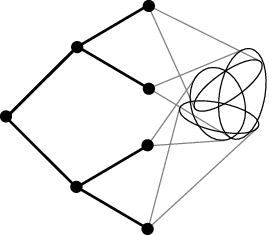
To rescue the situation we partition so that the first levels of from the root form the set of the cut-vertices . All other vertices make up the end shrubs . That is, , and .
We first embed the few cut-vertices . As will be much larger , following a strategy similar to the one above we ensure that all cut-vertices get correctly embedded. The next step is to make the transitions at the -th level from embedding cut-vertices to embedding shrubs . But since this step requires to exploit the structure of LKS graphs, we skip the details in the high-level overview here. For the sake of this simplified example, let us assume that all the cut-vertices are embedded in a set with
| (3.8) |
(where is a small constant).
For the point we wish to make here, it is more relevant to see how to complete the last part of our embedding, that is, how to embed a tree whose root is already embedded in a vertex . Let be the current (partial) image of . Further, we assume that throughout the entire process we have
| (3.9) |
where im is the image at that moment (and in particular, also at the end of the process). We explain how to achieve this property at the end.
We emphasize that at this moment we are working exclusively with the tree , i.e., any other tree is either completely embedded, or will be embedded only after we finish the embedding of . Suppose we are about to embed a vertex whose ancestor is already embedded in . We choose for the image of any (yet unused) vertex in the neighbourhood of , requiring that
| (3.10) |
This condition is very similar to our path-embedding procedure above, and can be proved in exactly the same way, using the fact that is -nowhere-dense. When is a cut-vertex, we need to combine this argument with (3.9).
Note that during our embedding will grow. However, is at most , which is much smaller than . Thus, for every vertex , when its time to be embedded comes, we still have a small degree to the partial image of the tree. Therefore can be embedded on a vertex that satisfies similarly as in (3.10).
Note that the trick here was to keep on working on one subtree , whose size is small enough to be negligible in comparison to the degree of the vertices in . So, by avoiding the vertices that have a considerable degree into , we actually also avoid those vertices that have a considerable degree into . Breaking up the tree into tiny shrubs was thus the key to successfully embedding it.
Let us now explain how to achieve (3.9). Instead of just embedding the tree we shall also reserve an equal amount of vertices in that are touched only exceptionally. More precisely, in a given step, instead of extending the embedding from a vertex to its two children, we first find four candidate vertices, and we randomly select two of them to host these children and insert the remaining two into a reserve set . Condition (3.10) is replaced by . This allows us to avoid not only but also when extending the embedding of . The only time the set may be used to host a vertex of some tree is when is the root of such a tree. Since the choice for the inclusion of vertices to was random, with high probability we have
where the term amounts to the roots for which the random choice is not used. Recall that . This together with (3.8) establishes (3.9).
3.7 Proof of the decomposition lemma
This subsection is devoted to the proof of the decomposition lemma (Lemma 3.13). In the proof, we start by extracting the edges of as many -dense spots from as possible; these together with the incident vertices will form the auxiliary graph . Most of the remaining edges will form the edge set of the graph . Next, we consider the intersections of the dense spots captured in . We apply the regularity lemma for locally dense graphs (Lemma 2.5) to the subgraph of that is spanned by the large intersections, and thus obtain . The other part of will be taken as the -avoiding set .
Setting up the parameters.
Defining and .
Given a graph , take a family of edge-disjoint -dense spots such that the resulting graph (which contains those vertices and edges that are contained in ) has the maximum number of edges.
Preparing for an application of the regularity lemma.
Let
| (3.13) |
where the latter partition refinement ranges over all . Let , , and . Furthermore let and .
Now, partition each set into subsets of cardinalities differing by at most one, and let be the set containing all the sets (for all ). Then for each we have that
| (3.14) |
Construct a graph on by making two vertices adjacent in if
- (A)
there is a dense spot such that and , and
- (B)
.
Note that it follows from the way was chosen that if then . On the other hand note that we do not necessarily have for the dense spot appearing in (A); just because there may be several such dense spots .
Regularising the dense spots in .
We apply Lemma 2.5 with parameters and as defined by (3.11) to the graphs and , together with the ensemble in the role of the sets , and partition of induced by
where .
Observe that is an -ensemble satisfying condition (2.2) of Lemma 2.5, by (3.14), by the choice of , and by (3.15). Thus we obtain integers and a family and a set such that, in particular, we have the following.
- (I)
We have for all .
- (II)
We have for any and for any , .
- (III)
For any and any , there is a set for which . We either have that , or and , or .
- (IV)
, where is the set of all edges of the graph contained in an -irregular pair , with , , .
Let be obtained from by erasing all vertices in , and all edges that lie in pairs which are irregular or of density at most . Then Properties 2, 3, 6 and 7 of Definition 3.7 are satisfied. Further, Lemma 2.10 implies (3.5). Together with (3.12) we obtain that the number of edges that are not captured by is at most .
The refinement in (3.13) guarantees that the bounded decomposition we have constructed respects the avoiding threshold .
The avoiding property of .
In order to see Property 8 of Definition 3.7, we have to show that is -avoiding with respect to . For this, let be such that . Let be the set of those vertices that are not contained in any dense spot for which . Our aim is to see that .
Let be the set of all dense spots with . Setting , the definition of trivially implies that . Now, by the definition of , we know that there are at most sets . Indeed, for each , either is a subset of , or of , or of . Thus,
| (3.16) |
3.8 Sparse decomposition of dense graphs
Let us explain our remark above that in the setting of a dense graph , Lemmas 3.14 and 3.15 produce a regularity partition in the usual sense. So, suppose that is an -vertex graph and has at least edges. This needs to be understood with the usual quantification “ is fixed and is large”.
Recall that when we inquire a -sparse decomposition, the parameters satisfy . The interplay between the parameters is quite complicated, and we do not give it here in full (see [HKP+d, p. ] for details). We justify with “parameter choice” any further relation we assume between them. Also, let us note that while our exact choice of parameters made in [HKP+d] are tailored for proving Theorem 1.3, we expect these relations to be satisfied in any application of Lemma 3.15, at least on the loose level we make use of them in this section.
First, we argue that it makes sense to set linear in , i.e., for some depending on only. Indeed, having would allow that all edges of are uncaptured in (3.6), which would make the lemma worthless. On the other hand, with we would have all vertices from ending up in the huge-degree set for which the sparse decomposition provides no structural information. Since , that would be a big loss of information, and thus often undesirable.
So, suppose now that , and suppose that is a -sparse decomposition of the dense graph . Since , we have that . Next, we argue that contains no vertices. Suppose on the contrary that it does. Then the minimum degree condition in Property 1 of Definition 3.7 tells us that has at least vertices of degrees at least each. Thus, . Since has at most vertices, and since (parameter choice), we get that contains at least one -dense spot, a contradiction to being nowhere-dense. Last, we claim, that . To this end, consider the set . We have , and thus the condition in Definition 3.6 applies. But there cannot exist any -dense spot as asserted in Definition 3.6 since for such a dense spot we would have , contradicting its required minimum degree condition. Thus, we conclude that all the vertices are exceptional in the sense of Definition 3.6, leading to the desired bound on .
To summarize, in the sparse decomposition , we have that , , are empty or almost empty. Thus, according to Definition 3.9, all the captured edges lie in the regularized graph . Property 4 of Definition 3.7 tells us that the clusters have size at least , that is, linear in the order of . Further, this property tells us that these clusters are of the same size. We conclude that is a regularization of in the sense of the original regularity lemma.
3.9 Algorithmic aspects of the decomposition lemma
Let us look back at the proof of the decomposition lemma (Lemma 3.13) and observe that we can get a bounded decomposition of any bounded-degree graph algorithmically in quasipolynomial time (in the order of the graph). Note that this in turn provides efficiently a sparse decomposition of any graph, since the initial step of splitting the graph into huge versus bounded degree vertices (cf. Lemma 3.2) can be done in polynomial time.
There are only two steps in the proof of Lemma 3.13 which need to be done algorithmically: the extraction of dense spots, and the simultaneous regularization of some dense pairs.
It will be more convenient to work with a relaxation of the notion of dense spots. We call a graph -thickthick graph if , and . The notion of thick graphs is a relaxation of dense spots, where the minimum degree condition is replaced by imposing a lower bound on the order, and the bipartiteness requirement is dropped. It can be verified that in our proof it is not important that the dense spots and the nowhere-dense graph are parametrized by the same constants, i.e., the entire proof would go through even if the spots in were -dense, and were -nowhere-dense for some . Each -thick graph gives (algorithmically) a -dense spot, and thus it is enough to extract thick graphs.
For the extraction of thick graphs we would need to efficiently answer the following: Given a number , find a number such that for an input number and an -vertex graph we can localize in a -thick graph if it contains a -thick graph, and output NO otherwise.55 5 We could additionally assume that due to the previous step of removing the set of huge degree vertices. Employing techniques from a deep paper of Arora, Frieze and Kaplan [AFK02], one can solve this problem in quasipolynomial time . This was communicated to us by Maxim Sviridenko. On the negative side, a truly polynomial algorithm seems to be out of reach, as Alon, Arora, Manokaran, Moshkovitz, and Weinstein [AAM+] reduced the problem to the notorious hidden clique problem, whose tractability has been open for twenty years.
Theorem 3.16 ([AAM+]).
If there is no polynomial time algorithm for solving the clique problem for a planted clique of size , then for any and there is no polynomial time algorithm that distinguishes between a graph on vertices containing a clique of size and a graph on vertices in which the densest subgraph on vertices has density at most .66 6 The result as stated in [AAM+] covers only the range . However there is a simple reduction by taking many disjoint copies of the general range to the restricted one.
Of course, Theorem 3.16 leaves some hope for a polynomial time algorithm when (which corresponds to ).
The regularity lemma can be made algorithmic [ADL+94]. The algorithm from [ADL+94] is based on index pumping-up, and thus applies even to the locally dense setting of Lemma 2.5.
It will turn out that the extraction of dense spots is the only obstruction to a polynomial time algorithm for Theorem 1.3. In [HKP+d], we sketch a truly polynomial time algorithm which avoids this step. It seems that the method sketched there is generally applicable for problems which employ sparse decompositions.
4 Acknowledgements
The work on this project lasted from the beginning of 2008 until 2014 and we are very grateful to the following institutions and funding bodies for their support.
During the work on this paper Hladký was also affiliated with Zentrum Mathematik, TU Munich and Department of Computer Science, University of Warwick. Hladký was funded by a BAYHOST fellowship, a DAAD fellowship, Charles University grant GAUK 202-10/258009, EPSRC award EP/D063191/1, and by an EPSRC Postdoctoral Fellowship during the work on the project.
Komlós and Szemerédi acknowledge the support of NSF grant DMS-0902241.
Piguet has been also affiliated with the Institute of Theoretical Computer Science, Charles University in Prague, Zentrum Mathematik, TU Munich, the Department of Computer Science and DIMAP, University of Warwick, and the school of mathematics, University of Birmingham. Piguet acknowledges the support of the Marie Curie fellowship FIST, DFG grant TA 309/2-1, a DAAD fellowship, Czech Ministry of Education project 1M0545, EPSRC award EP/D063191/1, and the support of the EPSRC Additional Sponsorship, with a grant reference of EP/J501414/1 which facilitated her to travel with her young child and so she could continue to collaborate closely with her coauthors on this project. This grant was also used to host Stein in Birmingham. Piguet was supported by the European Regional Development Fund (ERDF), project “NTIS - New Technologies for Information Society”, European Centre of Excellence, CZ.1.05/1.1.00/02.0090.
Stein was affiliated with the Institute of Mathematics and Statistics, University of São Paulo, the Centre for Mathematical Modeling, University of Chile and the Department of Mathematical Engineering, University of Chile. She was supported by a FAPESP fellowship, and by FAPESP travel grant PQ-EX 2008/50338-0, also CMM-Basal, FONDECYT grants 11090141 and 1140766. She also received funding by EPSRC Additional Sponsorship EP/J501414/1.
We enjoyed the hospitality of the School of Mathematics of University of Birmingham, Center for Mathematical Modeling, University of Chile, Alfréd Rényi Institute of Mathematics of the Hungarian Academy of Sciences and Charles University, Prague, during our long term visits.
The yet unpublished work of Ajtai, Komlós, Simonovits, and Szemerédi on the Erdős–Sós Conjecture was the starting point for our project, and our solution crucially relies on the methods developed for the Erdős-Sós Conjecture. Hladký, Piguet, and Stein are very grateful to the former group for explaining them those techniques.
Hladký would like to thank Maxim Sviridenko for discussion on the algorithmic aspects of the problem.
A doctoral thesis entitled Structural graph theory submitted by Hladký in September 2012 under the supervision of Daniel Král at Charles University in Prague is based on the series of the papers [HKP+a, HKP+b, HKP+c, HKP+d]. The texts of the two works overlap greatly. We are grateful to PhD committee members Peter Keevash and Michael Krivelevich. Their valuable comments are reflected in the series.
We thank the referees for their very detailed remarks.
The contents of this publication reflects only the authors’ views and not necessarily the views of the European Commission of the European Union.
mathsymbolsSymbol index \printindexgeneralGeneral index
References
- [AAM+] N. Alon, S. Arora, R. Manokaran, D. Moshkovitz, and O. Weinstein. Inapproximability of densest -subgraph from average case hardness. Available via http://people.csail.mit.edu/dmoshkov/papers/.
- [ADL+94] N. Alon, R. Duke, H. Lefmann, V. Rödl, and R. Yuster. The algorithmic aspects of the regularity lemma. J. Algorithms, 16:80–109, 1994.
- [AFK02] S. Arora, A. Frieze, and H. Kaplan. A new rounding procedure for the assignment problem with applications to dense graph arrangement problems. Math. Program., 92(1):1–36, 2002.
- [AKS81] M. Ajtai, J. Komlós, and E. Szemerédi. The longest path in a random graph. Combinatorica, 1(1):1–12, 1981.
- [AKS95] M. Ajtai, J. Komlós, and E. Szemerédi. On a conjecture of Loebl. In Graph theory, combinatorics, and algorithms, Vol. 1, 2 (Kalamazoo, MI, 1992), Wiley-Intersci. Publ., pages 1135–1146. Wiley, New York, 1995.
- [AKS07] N. Alon, M. Krivelevich, and B. Sudakov. Embedding nearly-spanning bounded degree trees. Combinatorica, 27(6):629–644, 2007.
- [AKSS] M. Ajtai, J. Komlós, M. Simonovits, and E. Szemerédi. Erdős-Sós conjecture. In preparation.
- [AKSV14] P. Allen, P. Keevash, B. Sudakov, and J. Verstraete. Turán numbers of bipartite graphs plus an odd cycle. J. Combin. Theory Ser. B, 106:134–162, 2014.
- [BCLR89] S. N. Bhatt, F. R. K. Chung, F. T. Leighton, and A. L. Rosenberg. Universal graphs for bounded-degree trees and planar graphs. SIAM J. Discrete Math., 2(2):145–155, 1989.
- [BCPS10] J. Balogh, B. Csaba, M. Pei, and W. Samotij. Large bounded degree trees in expanding graphs. Electron. J. Combin., 17(1):Research Paper 6, 9, 2010.
- [BD96] S. Brandt and E. Dobson. The Erdős–Sós conjecture for graphs of girth . Discr. Math., 150:411–414, 1996.
- [BJ] O. Barr and R. Johansson. Another Note on the Loebl–Komlós–Sós Conjecture. Research reports no. 22, (1997), Umeå University, Sweden.
- [BLW00] C. Bazgan, H. Li, and M. Woźniak. On the Loebl-Komlós-Sós conjecture. J. Graph Theory, 34(4):269–276, 2000.
- [Bol84] B. Bollobás. The evolution of sparse graphs. In Graph theory and combinatorics (Cambridge, 1983), pages 35–57. Academic Press, London, 1984.
- [BS97] I. Benjamini and O. Schramm. Every graph with a positive Cheeger constant contains a tree with a positive Cheeger constant. Geom. Funct. Anal., 7(3):403–419, 1997.
- [CLNGS10] B. Csaba, I. Levitt, J. Nagy-György, and E. Szemeredi. Tight bounds for embedding bounded degree trees. In Fete of combinatorics and computer science, volume 20 of Bolyai Soc. Math. Stud., pages 95–137. János Bolyai Math. Soc., Budapest, 2010.
- [Coo09] O. Cooley. Proof of the Loebl-Komlós-Sós conjecture for large, dense graphs. Discrete Math., 309(21):6190–6228, 2009.
- [Die05] R. Diestel. Graph theory, volume 173 of Graduate Texts in Mathematics. Springer-Verlag, Berlin, third edition, 2005.
- [Dob02] E. Dobson. Constructing trees in graphs whose complement has no . Combin. Probab. Comput., 11(4):343–347, 2002.
- [EFLS95] P. Erdős, Z. Füredi, M. Loebl, and V. T. Sós. Discrepancy of trees. Studia Sci. Math. Hungar., 30(1-2):47–57, 1995.
- [EL] G. Elek and G. Lippner. An analogue of the Szemerédi regularity lemma for bounded degree graphs. Manuscript (arXiv:0809.2879).
- [FdlV79] W. Fernandez de la Vega. Long paths in random graphs. Studia Sci. Math. Hungar., 14(4):335–340, 1979.
- [FNP] A. Ferber, R. Nenadov, and U. Peter. Universality of random graphs and rainbow embedding. to appear in Random Structures Algorithms, arXiv:1311.7063.
- [FP87] J. Friedman and N. Pippenger. Expanding graphs contain all small trees. Combinatorica, 7(1):71–76, 1987.
- [GG67] L. Gerencsér and A. Gyárfás. On Ramsey-type problems. Ann. Univ. Sci. Budapest. Eötvös Sect. Math., 10:167–170, 1967.
- [Har72] F. Harary. Recent results on generalized Ramsey theory for graphs. In Graph theory and applications (Proc. Conf., Western Michigan Univ., Kalamazoo, Mich., 1972; dedicated to the memory of J. W. T. Youngs), pages 125–138. Lecture Notes in Math., Vol. 303. Springer, Berlin, 1972.
- [Hax01] P. E. Haxell. Tree embeddings. J. Graph Theory, 36(3):121–130, 2001.
- [HK95] P. E. Haxell and Y. Kohayakawa. The size-Ramsey number of trees. Israel J. Math., 89(1-3):261–274, 1995.
- [HKP+a] J. Hladký, J. Komlós, D. Piguet, M. Simonovits, M. Stein, and E. Szemerédi. The approximate Loebl–Komlós–Sós Conjecture I: The sparse decomposition. Manuscript (arXiv:1408.3858).
- [HKP+b] J. Hladký, J. Komlós, D. Piguet, M. Simonovits, M. Stein, and E. Szemerédi. The approximate Loebl–Komlós–Sós Conjecture II: The rough structure of LKS graphs. Manuscript (arXiv:1408.3871).
- [HKP+c] J. Hladký, J. Komlós, D. Piguet, M. Simonovits, M. Stein, and E. Szemerédi. The approximate Loebl–Komlós–Sós Conjecture III: The finer structure of LKS graphs. Manuscript (arXiv:1408.3866).
- [HKP+d] J. Hladký, J. Komlós, D. Piguet, M. Simonovits, M. Stein, and E. Szemerédi. The approximate Loebl–Komlós–Sós Conjecture IV: Embedding techniques and the proof of the main result. Manuscript (arXiv:1408.3870).
- [HKS12] D. Hefetz, M. Krivelevich, and T. Szabó. Sharp threshold for the appearance of certain spanning trees in random graphs. Random Structures and Algorithms, 41:391–412, 2012.
- [Hla] J. Hladký. Szemerédi Regularity Lemma and its applications in combinatorics. MSc. Thesis, Charles University in Prague, 2008, available via http://homepages.warwick.ac.uk/maskai/papers.html.
- [HLT02] P. E. Haxell, T. Luczak, and P. W. Tingley. Ramsey numbers for trees of small maximum degree. Combinatorica, 22(2):287–320, 2002. Special issue: Paul Erdős and his mathematics.
- [HP15] J. Hladký and D. Piguet. Loebl–Komlós–Sós Conjecture: dense case. J. Combin. Theory Ser. B, 2015. http://dx.doi.org/10.1016/j.jctb.2015.07.004.
- [HPS+15] J. Hladký, D. Piguet, M. Simonovits, M. Stein, and E. Szemerédi. The approximate Loebl–Komlós–Sós conjecture and embedding trees in sparse graphs. Electron. Res. Ann. Math. Sci., 22:1–11, 2015.
- [JKS12] D. Johannsen, M. Krivelevich, and W. Samotij. Expanders are universal for the class of all spanning trees. In Proceedings of the Twenty-Third Annual ACM-SIAM Symposium on Discrete Algorithms, SODA ’12, pages 1539–1551. SIAM, 2012.
- [JKV08] A. Johansson, J. Kahn, and V. Vu. Factors in random graphs. Random Structures Algorithms, 33(1):1–28, 2008.
- [KMO11a] D. Kühn, R. Mycroft, and D. Osthus. An approximate version of Sumner’s universal tournament conjecture. J. Combin. Theory Ser. B, 101(6):415–447, 2011.
- [KMO11b] D. Kühn, R. Mycroft, and D. Osthus. A proof of Sumner’s universal tournament conjecture for large tournaments. Proc. Lond. Math. Soc. (3), 102(4):731–766, 2011.
- [KO09] D. Kühn and D. Osthus. Embedding large subgraphs into dense graphs. In Surveys in combinatorics 2009, volume 365 of London Math. Soc. Lecture Note Ser., pages 137–167. Cambridge Univ. Press, Cambridge, 2009.
- [Koh97] Y. Kohayakawa. Szemerédi’s regularity lemma for sparse graphs. In Foundations of computational mathematics (Rio de Janeiro, 1997), pages 216–230. Springer, Berlin, 1997.
- [Kri10] M. Krivelevich. Embedding spanning trees in random graphs. SIAM J. Discrete Math., 24(4):1495–1500, 2010.
- [KS83] J. Komlós and E. Szemerédi. Limit distribution for the existence of Hamiltonian cycles in a random graph. Discrete Math., 43(1):55–63, 1983.
- [KS96] J. Komlós and M. Simonovits. Szemerédi’s regularity lemma and its applications in graph theory. In Combinatorics, Paul Erdős is eighty, Vol. 2 (Keszthely, 1993), volume 2 of Bolyai Soc. Math. Stud., pages 295–352. János Bolyai Math. Soc., Budapest, 1996.
- [KSS01] J. Komlós, G. N. Sárközy, and E. Szemerédi. Spanning trees in dense graphs. Combin. Probab. Comput., 10(5):397–416, 2001.
- [Mona] R. Montgomery. Embedding bounded degree spanning trees in random graphs. Manuscript (arXiv:1405.6559).
- [Monb] R. Montgomery. Sharp threshold for embedding combs and other spanning trees in random graphs. Manuscript (arXiv:1405.6560).
- [MS] M. Matsumoto and S. Sakamoto. Constructing trees in graphs whose complement has no one-leaved . Preprint 2009.
- [Pós76] L. Pósa. Hamiltonian circuits in random graphs. Discrete Math., 14(4):359–364, 1976.
- [PS08] D. Piguet and M. J. Stein. Loebl-Komlós-Sós conjecture for trees of diameter 5. Electron. J. Combin., 15(1):Research Paper 106, 11 pp. (electronic), 2008.
- [PS12] D. Piguet and M. J. Stein. An approximate version of the Loebl-Komlós-Sós conjecture. J. Combin. Theory Ser. B, 102(1):102–125, 2012.
- [Sco11] A. Scott. Szemerédi’s regularity lemma for matrices and sparse graphs. Combin. Probab. Comput., 20(3):455–466, 2011.
- [Sof00] S. N. Soffer. The Komlós-Sós conjecture for graphs of girth 7. Discrete Math., 214(1-3):279–283, 2000.
- [Sun07] L. Sun. On the Loebl-Komlós-Sós conjecture. Australas. J. Combin., 37:271–275, 2007.
- [SV10] B. Sudakov and J. Vondrák. A randomized embedding algorithm for trees. Combinatorica, 30(4):445–470, 2010.
- [SW97] J.-F. Saclé and M. Woźniak. A note on the Erdős–Sós conjecture for graphs without . J. Combin. Theory (Series B), 70(2):229–234, 1997.
- [Sze78] E. Szemerédi. Regular partitions of graphs. In Problèmes combinatoires et théorie des graphes (Colloq. Internat. CNRS, Univ. Orsay, Orsay, 1976), volume 260 of Colloq. Internat. CNRS, pages 399–401. CNRS, Paris, 1978.
- [Woź96] M. Woźniak. On the Erdős–Sós conjecture. J. Graph Theory, 21(2):229–234, 1996.
- [Zha11] Y. Zhao. Proof of the conjecture for large . Electron. J. Combin., 18(1):Paper 27, 61, 2011.