∎

On the expected number of equilibria in a multi-player multi-strategy evolutionary game

Manh Hong Duong Affiliation: Mathematics Institute, Zeeman Building, University of Warwick, Coventry CV4 7AL, UK. E-mail: m.h.duong@warwick.ac.uk The Anh Han Affiliation: School of Computing, Teesside University, Borough Road, Middlesbrough, UK TS1 3BA E-mail: T.Han@tees.ac.uk

Received: date / Accepted: date

Abstract

In this paper, we analyse the mean number $E(n,d)$ of internal equilibria in a general $d$ -player $n$ -strategy evolutionary game where the agents’ payoffs are normally distributed. First, we give a computationally implementable formula for the general case. Next, we characterize the asymptotic behaviour of $E(2,d)$ , estimating its lower and upper bounds as $d$ increases. Then we provide a closed formula for $E(n,2)$ . Two important consequences are obtained from this analysis. On the one hand, we show that in both cases the probability of seeing the maximal possible number of equilibria tends to zero when $d$ or $n$ respectively goes to infinity. On the other hand, we demonstrate that the expected number of stable equilibria is bounded within a certain interval. Finally, for larger $n$ and $d$ , numerical results are provided and discussed.

Keywords:

Evolutionary game multi-player games multiple strategies random polynomialsnumber of equilibriarandom games.

1 Introduction

Evolutionary game theory is the suitable mathematical framework whenever there is frequency dependent selection – the fitness of an individual does not only depend on its strategy, but also on the composition of the population in relation with (multiple) other strategies MS (82); HS (98); Now (06). The payoff from the games is interpreted as individual fitness, naturally leading to a dynamical approach. As in classical game theory with the Nash equilibrium MB (05); McL (05), the analysis of properties of equilibrium points in evolutionary game theory has been of special interest MS (82); BCV (97); GT (10). Herein, equilibrium points of a dynamical system predict the composition of strategy frequencies where all the strategies have the same average fitness. Biologically, these points can predict a co-existence of different types in a population and the maintenance of polymorphism.

Recently, some attention has been paid to both numerical and analytical studies of equilibrium points and their stability in random evolutionary games GT (10); HTG (12). The focus was on analyzing the probability of observing a certain number of equilibria (whether counting all equilibria or only the stable ones) if the payoff entries are randomly drawn. This probability allows one to predict the complexity of the interactions as the number of strategies and the number of players in the game increase, especially when the environments are unknown or changing rapidly over time FH (92); GRLD (09). Furthermore, these studies have paid substantial attention to the maximal number of equilibrium points and the attainability of the patterns of evolutionarily stable strategies, as knowing them is insightful, and historically they have been studied extensively, not only in classical and evolutionary game theory, but also in other fields such as population genetics MS (82); Kar (80); VC88a (); VC88b (); KF (70); VC88c (); Hai (89); BCV (94); BCV (93); BCV (97); Alt (10); GT (10); HTG (12); BR (13). However, as the studies deal with the concrete numbers of equilibrium points, they have needed to take a direct approach that consists of solving a system of polynomial equations, the degree of which increases with the number of players in a game. As such, the mathematical analysis was mostly restricted to evolutionary games with a small number of players, due to the impossibility of solving general polynomial equations of a high degree Abe (24); HTG (12).

In this paper, we ask instead the question: what is the mean or expected number of equilibria that one can observe if the payoff matrix entries of the game are randomly drawn? Knowing the mean number of equilibria not only gives important insights into the overall complexity of the interactions as the number of participating players in the game and the potential strategies that the players can adopt are magnified. It also enables us to predict the boundaries of the concrete numbers of (stable) equilibrium points such as the maximal one as we show later on in the paper. By connecting to the theory of random polynomials EK (95), we first provide an exact, computationally implementable, formula for the expected number of equilibria in a general multi-player multi-strategy random game when the payoff entries are normally distributed. Secondly, we derive lower and upper bounds of such a formula for the case of two-player games and provide an explicit formula for the case of two-strategy games. As a consequence, we can derive similar bounds when considering only equilibrium points that are stable. Finally, numerical results are provided and discussed when there are more players and strategies.

The rest of the paper is structured as follows. In Section 2 we introduce the models and methods: the replicator equation in evolution game theory and the random polynomial theory are summarized in Sections 2.1 and 2.2, respectively. The link between them, which is a major aspect of our method, is described in Section 2.3. The main results of this paper are presented in Section 3, starting with two-strategy games in Section 3.1, then with two-player games in Section 3.2, and lastly, with the general case of games with arbitrary numbers of players and strategies in Section 3.3. We compare our results with related ones in the literature and discuss some future directions in Section 4. Finally, some detailed computations are given in the Appendix.

2 Models and Methods

2.1 Evolutionary game theory and replicator dynamics

The classical approach to evolutionary games is replicator dynamics TJ (78); Zee (80); HS (98); SS (83); Now (06), describing that whenever a strategy has a fitness larger than the average fitness of the population, it is expected to spread. Formally, let us consider an infinitely large population with $n$ strategies, numerated from 1 to $n$ . They have frequencies $x_{i}$ , $1\leq i\leq n$ , respectively, satisfying that $0\leq x_{i}\leq 1$ and $\sum_{i=1}^{n}x_{i}=1$ . The interaction of the individuals in the population is in randomly selected groups of $d$ participants, that is, they play and obtain their fitness from $d$ -player games. We consider here symmetrical games (e.g. the public goods games and their generalizations Har (68); HDMHS (02); SSP (08); PSSS (09); HMPLss ()) in which the order of the participants is irrelevant. Let $\alpha^{i_{0}}_{i_{1},\ldots,i_{d-1}}$ be the payoff of the focal player, where $i_{0}$ ( $1\leq i_{0}\leq n$ ) is the strategy of the focal player, and let $i_{k}$ (with $1\leq i_{k}\leq n$ and $1\leq k\leq d-1$ ) be the strategy of the player in position $k$ . These payoffs form a $(d-1)$ -dimensional payoff matrix GT (10), which satisfies (because of the game symmetry)

\alpha^{i_{0}}_{i_{1},\ldots,i_{d-1}}=\alpha^{i_{0}}_{i_{1}^{\prime},\ldots,i_{d-1}^{\prime}},

(1)

whenever $\{i_{1}^{\prime}\ldots,i_{d-1}^{\prime}\}$ is a permutation of $\{i_{1}\ldots,i_{d-1}\}$ . This means that only the fraction of each strategy in the game matters.

The average payoff or fitness of the focal player is given by

\pi_{i_{0}}=\sum\limits_{i_{1},\ldots,i_{d-1}=1}^{n}\alpha^{i_{0}}_{i_{1},\ldots,i_{d-1}}\prod\limits_{k=1}^{d-1}x_{i_{k}}.

(2)

By abuse of notation, let us denote $\alpha^{i_{0}}_{k_{1},...,k_{n}}:=\alpha^{i_{0}}_{i_{1},\ldots,i_{d-1}}$ , where $k_{i}$ , $1\leq i\leq n$ , with $\sum^{n}_{i=1}k_{i}=d-1$ , is the number of players using strategy $i$ in $\{i_{1},\ldots,i_{d-1}\}$ . Hence, from Equation (1), the fitness of strategy $i_{0}$ can be rewritten as follows

\pi_{i_{0}}=\sum\limits_{\begin{subarray}{c}0\leq k_{1},...,k_{n}\leq d-1,\\ \sum\limits^{n}_{i=1}k_{i}=d-1\end{subarray}}\alpha^{i_{0}}_{k_{1},...,k_{n}}\begin{pmatrix}d-1\\ k_{1},...,k_{n}\end{pmatrix}\prod\limits_{i=1}^{n}x_{i}^{k_{i}}\quad\text{ for }i_{0}=1,\dots,n,

(3)

where $\begin{pmatrix}d-1\\ k_{1},\dots,k_{n}\end{pmatrix}=\frac{(d-1)!}{\prod\limits_{k=1}^{n}k_{i}!}$ are the multinomial coefficients.

Now the replicator equations for games with $n$ strategies can be written as follows HS (98); Sig (10)

\dot{x_{i}}=x_{i}\left(\pi_{i}-\langle\pi\rangle\right)\quad\quad\text{ for }i=1,\dots,n-1,

(4)

where $\langle\pi\rangle=\sum^{n}_{k=1}x_{k}\,\pi_{k}$ is the average payoff of the population. The equilibrium points of the system are given by the points $(x_{1},\dots,x_{n})$ satisfying the condition that the fitness of all strategies are the same. That is, they are represented by solutions of the system of equations

\pi_{i}=\pi_{n}\quad\text{ for all }1\leq i\leq n-1.

(5)

Subtracting from each of the equations the term $\pi_{n}$ we obtain a system of $n-1$ polynomials of degree $d-1$

\sum\limits_{\begin{subarray}{c}0\leq k_{1},...,k_{n}\leq d-1,\\ \sum^{n}\limits_{i=1}k_{i}=d-1\end{subarray}}\beta^{i}_{k_{1},...,k_{n-1}}\begin{pmatrix}d-1\\ k_{1},...,k_{n}\end{pmatrix}\prod\limits_{i=1}^{n}x_{i}^{k_{i}}=0\quad\text{ for }i=1,\dots,n-1,

(6)

where $\beta^{i}_{k_{1},...,k_{n-1}}:=\alpha^{i}_{k_{1},...,k_{n}}-\alpha^{n}_{k_{1},...,k_{n}}$ . Assuming that all the payoff entries have the same probability distribution, then all $\beta^{i}_{k_{1},...,k_{n-1}}$ , $i=1,\dots,n-1$ , have symmetric distributions, i.e. with mean 0 (see also the proof in HTG (12)).

In the following analysis, we focus on internal equilibrium points GT (10); HTG (12), i.e. $0<x_{i}<1$ for all $1\leq i\leq n-1$ . Hence, by using the transformation $y_{i}=\frac{x_{i}}{x_{n}}$ , with $0<y_{i}<+\infty$ and $1\leq i\leq n-1$ , dividing the left hand side of the above equation by $x_{n}^{d-1}$ we obtain the following equation in terms of $(y_{1},\ldots,y_{n-1})$ that is equivalent to (6)

\sum\limits_{\begin{subarray}{c}0\leq k_{1},...,k_{n-1}\leq d-1,\\ \sum\limits^{n-1}_{i=1}k_{i}\leq d-1\end{subarray}}\beta^{i}_{k_{1},...,k_{n-1}}\begin{pmatrix}d-1\\ k_{1},...,k_{n}\end{pmatrix}\prod\limits_{i=1}^{n-1}y_{i}^{k_{i}}=0\quad\quad\text{ for }i=1,\dots,n-1.

(7)

As stated, one of the main goals of this article is to compute the expected number of (internal) equilibria in a general $n$ -strategy $d$ -player random evolutionary game. That consists in computing the expected number of solutions $(y_{1},\dots,y_{n-1})\in{\mathbb{R}_{+}}^{n-1}$ of the system of $(n-1)$ polynomials of degree $(d-1)$ in (7). Furthermore, herein our analysis focuses on payoff matrices with normally distributed entries. It is known that, even for $n=2$ , it is impossible to analytically solve the system whenever $d>5$ Abe (24), as seen in HTG (12). Hence, it is not feasible to use this direct approach of analytically solving the system if one wants to deal with games with a large number of players and with multiple strategies. In this work, we address this issue by connecting to the theory of random polynomials described in the following section.

2.2 Random polynomial theory

Keeping the form of Eq. (7) in mind, we consider a system of $n-1$ random polynomials of degree $d-1$ ,

\sum\limits_{\begin{subarray}{c}0\leq k_{1},...,k_{n-1}\leq d-1,\\ \sum^{n-1}_{i=1}k_{i}\leq d-1\end{subarray}}a^{i}_{k_{1},...,k_{n-1}}\prod\limits_{i=1}^{n-1}y_{i}^{k_{i}}=0\quad\quad\text{ for }i=1,\dots,n-1,

(8)

where $a^{i}_{k_{1},...,k_{n-1}}$ are independent and identically distributed (i.i.d.) multivariate normal random vectors with mean zero and covariance matrix $C$ . Denote by $v(y)$ the vector whose components are all the monomials $\big\{\prod\limits_{i=1}^{n-1}y_{i}^{k_{i}}\big\}$ where $0\leq k_{i}\leq d-1$ and $\sum\limits_{i=1}^{n-1}k_{i}\leq d-1$ . Let $A$ denote the random matrix whose $i-$ th row contains all coefficients $a^{i}_{k_{1},\ldots,k_{n-1}}$ . Then (8) can be re-written as

Av(y)=0.

(9)

The following theorem is the starting point of the analysis of this paper.

Theorem 2.1

(EK, 95, Theorem 7.1) Let $U$ be any measurable subset of $\mathbb{R}^{n-1}$ . Assume that the rows of $A$ are i.i.d. multivariate normal random vectors with mean zero and covariance matrix $C$ . The expected number of real roots of the system of equations (9) that lie in the set $U$ is given by

\pi^{-\frac{n}{2}}\Gamma\left(\frac{n}{2}\right)\int_{U}\left(\det\left[\frac{\partial^{2}}{\partial x_{i}\partial y_{j}}(\log v(x)^{T}Cv(y))\big|_{y=x=t}\right]_{ij}\right)^{\frac{1}{2}}\,dt.

2.3 From random polynomial theory to evolutionary game theory

Let $E(n,d)$ be the number of internal equilibria in a $d-$ player random game with $n$ strategies. As has been shown in Section 2.1, $E(n,d)$ is the same as the number of positive solutions of Eq. (7). We will apply Theorem 2.1 with $a^{i}_{k_{1},...,k_{n-1}}=\beta^{i}_{k_{1},...,k_{n-1}}\begin{pmatrix}d-1\\ k_{1},...,k_{n}\end{pmatrix}$ and $U=[0,\infty)^{n-1}\subset\mathbb{R}^{n-1}$ .

Suppose that all $\beta^{i}_{k_{1},...,k_{n-1}}$ are Gaussian distributions with mean $0$ and variance $1$ , then for each $i$ ( $1\leq i\leq n-1$ ), $A^{i}=\left\{\beta^{i}_{k_{1},...,k_{n-1}}\begin{pmatrix}d-1\\ k_{1},...,k_{n}\end{pmatrix}\right\}$ is a multivariate normal random vector with mean zero and covariance matrix $C$ given by

C=\mathrm{diag}\left(\begin{pmatrix}d-1\\ k_{1},...,k_{n}\end{pmatrix}^{2}\right)_{0\leq k_{i}\leq d-1,~\sum\limits_{i=1}^{n-1}k_{i}\leq d-1}.

(10)

We obtain the following lemma, which is a direct application of Theorem 2.1.

Lemma 1

Assume that $\{A^{i}\}_{1\leq i\leq n-1}$ are independent normal random vectors with mean zero and covariance matrix $C$ as in (10). The expected number of internal equilibria in a d-player n-strategy random game is given by

E(n,d)=\pi^{-\frac{n}{2}}\Gamma\left(\frac{n}{2}\right)\underbrace{\int_{0}^{\infty}\ldots\int_{0}^{\infty}}_{n-1\,\text{times}}\left(\det\left[\frac{\partial^{2}}{\partial x_{i}y_{j}}(\log v(x)^{T}Cv(y))\big|_{y=x=t}\right]_{ij}\right)^{\frac{1}{2}}\,dt,

(11)

where

v(x)^{T}Cv(y)=\sum\limits_{\begin{subarray}{c}0\leq k_{1},...,k_{n-1}\leq d-1,\\ \sum\limits^{n-1}_{i=1}k_{i}\leq d-1\end{subarray}}\begin{pmatrix}d-1\\ k_{1},\ldots,k_{n}\end{pmatrix}^{2}\prod\limits_{i=1}^{n}x_{i}^{k_{i}}y_{i}^{k_{i}}.

(12)

Denote by $L$ the matrix with entries

\displaystyle L_{ij}

\displaystyle=\frac{\partial^{2}}{\partial x_{i}y_{j}}(\log v(x)^{T}Cv(y))\big|_{y=x=t},

then $E(n,d)$ can be written as

E(n,d)=\pi^{-\frac{n}{2}}\Gamma\left(\frac{n}{2}\right)\underbrace{\int_{0}^{\infty}\ldots\int_{0}^{\infty}}_{n-1\,\text{times}}\left(\det L\right)^{\frac{1}{2}}dt.

(13)

It has been shown that a $d$ -player $n$ -strategy game has at most $(d-1)^{n-1}$ isolated internal equilibria (and this bound is sharp) HTG (12). We denote by $p_{i}$ , $1\leq i\leq(d-1)^{n-1}$ , the probability that the game has exactly $i$ such equilibria. Then $E(n,d)$ can also be defined through $p_{i}$ as follows

E(n,d)=\sum_{i=1}^{(d-1)^{n-1}}i\cdot p_{i}.

(14)

3 Results

We start with the case where there are two strategies ( $n=2$ ), analytically deriving the upper and lower bounds for $E(2,d)$ . Next we derive exact results for games with two players ( $d=2$ ). Finally, we provide numerical results and discussion for the general case with an arbitrary number of players and strategies. For ease of representation, we start by assuming that the coefficients $\beta^{i}_{k_{1},\ldots,k_{n-1}}$ are standard normal distributions. We then show that the results do not change if they have arbitrary identical normal distributions.

3.1 Multi-player two-strategy games

We first consider games with an arbitrary number of players, but having only two strategies, i.e. $n=2$ . In this case, Equation (7) is simplified to the following univariate polynomial equation of degree $d-1$ with $y\in\mathbb{R}_{+}$

\sum\limits_{k=0}^{d-1}\beta_{k}\begin{pmatrix}d-1\\ k\end{pmatrix}y^{k}=0.

(15)

The following lemma describes a closed form of $E(2,d)$ .

Lemma 2

Assume that $\beta_{k}$ are independent Gaussian distributions with variance $1$ and mean $0$ . Then the number of internal equilibria, $E(2,d)$ , in a $d-$ player random game with two strategies is given by

E(2,d)=\int_{0}^{\infty}f(t)\,dt,

(16)

where

f(t)=\frac{1}{\pi}\left[\frac{\sum\limits_{k=1}^{d-1}k^{2}\begin{pmatrix}d-1\\ k\end{pmatrix}^{2}t^{2(k-1)}}{\sum\limits_{k=0}^{d-1}\begin{pmatrix}d-1\\ k\end{pmatrix}^{2}t^{2k}}-\left(\frac{\sum\limits_{k=1}^{d-1}k\begin{pmatrix}d-1\\ k\end{pmatrix}^{2}t^{2k-1}}{\sum\limits_{k=0}^{d-1}\begin{pmatrix}d-1\\ k\end{pmatrix}^{2}t^{2k}}\right)^{2}\right]^{\frac{1}{2}}.

(17)

Proof

Since $\beta_{k}$ has Gaussian distribution with variance $1$ and mean $0$ , $\beta_{k}\begin{pmatrix}d-1\\ k\end{pmatrix}$ has Gaussian distribution with variance $\begin{pmatrix}d-1\\ k\end{pmatrix}^{2}$ and mean $0$ . According to Lemma 1, the equality (16) holds with

f(t)=\frac{1}{\pi}\left[\frac{\partial^{2}}{\partial x\partial y}\left(\log v(x)^{T}Cv(y)\right)\Big|_{y=x=t}\right]^{\frac{1}{2}},

(18)

where the vector $v$ and the matrix $C$ (covariance matrix) are given by

v(x)=\begin{pmatrix}1\\ x\\ \vdots\\ x^{d-1}\end{pmatrix},\quad C=(C_{ij})_{i,j=1,\ldots,d-1}\quad\text{with}~~C_{ij}=\delta_{ij}\begin{pmatrix}d-1\\ i\end{pmatrix}\begin{pmatrix}d-1\\ j\end{pmatrix},

(19)

where $\delta_{ij}$ is the Kronecker notation,

\delta_{ij}=\begin{cases}1\quad\textrm{if}\quad i=j,\\ 0\quad\textrm{if}\quad i\neq j.\end{cases}

A straightforward calculation gives

v(x)^{T}Cv(y)=\sum\limits_{k=0}^{d-1}\begin{pmatrix}d-1\\ k\end{pmatrix}^{2}x^{k}y^{k},

and

	$\displaystyle\frac{\partial^{2}}{\partial x\partial y}\left(\log v(x)^{T}Cv(y)\right)$	$\displaystyle=\frac{\sum\limits_{k=1}^{d-1}k^{2}\begin{pmatrix}d-1\\ k\end{pmatrix}^{2}x^{k-1}y^{k-1}}{\sum\limits_{k=0}^{d-1}\begin{pmatrix}d-1\\ k\end{pmatrix}^{2}x^{k}y^{k}}$
		$\displaystyle\ \ -\frac{\left(\sum\limits_{k=1}^{d-1}k\begin{pmatrix}d-1\\ k\end{pmatrix}^{2}x^{k}y^{k-1}\right)\left(\sum\limits_{k=1}^{d-1}k\begin{pmatrix}d-1\\ k\end{pmatrix}^{2}x^{k-1}y^{k}\right)}{\left(\sum\limits_{k=0}^{d-1}\begin{pmatrix}d-1\\ k\end{pmatrix}^{2}x^{k}y^{k}\right)^{2}}.$

Substituting this expression into (18), we obtain (17).

Example 1

For the cases $d=2$ and $d=3$ , we have

		$\displaystyle E(2,2)=\frac{1}{\pi}\int_{0}^{\infty}\frac{1}{1+t^{2}}\,dt=\frac{1}{\pi}\lim_{t\rightarrow+\infty}\tan^{-1}(t)=0.5,$
		$\displaystyle E(2,3)=\frac{2}{\pi}\int_{0}^{\infty}\frac{\sqrt{t^{4}+t^{2}+1}}{t^{4}+4t^{2}+1}\,dt\approx 0.77.$

The following proposition presents some properties of the density function $f(t)$ , which will be used later for estimating the asymptotic behaviour of $E(2,d)$ .

Proposition 1

The following properties hold

f(t)=\frac{d-1}{\pi}\frac{\sqrt{\sum\limits_{k=0}^{2d-4}a_{k}\,t^{2k}}}{{\sum\limits_{k=0}^{d-1}\begin{pmatrix}d-1\\ k\end{pmatrix}^{2}t^{2k}}},

(20)

where

		$\displaystyle a_{k}=\sum\limits_{\begin{subarray}{c}1\leq i\leq d-1\\ 1\leq j\leq d-2\\ i+j=k\end{subarray}}\begin{pmatrix}d-1\\ i\end{pmatrix}^{2}\begin{pmatrix}d-2\\ j\end{pmatrix}^{2}-\sum\limits_{\begin{subarray}{c}1\leq i^{\prime}\leq d-2\\ 1\leq j^{\prime}\leq d-2\\ i^{\prime}+j^{\prime}=k\end{subarray}}\begin{pmatrix}d-2\\ i^{\prime}\end{pmatrix}\begin{pmatrix}d-1\\ i^{\prime}+1\end{pmatrix}\begin{pmatrix}d-2\\ j^{\prime}\end{pmatrix}\begin{pmatrix}d-1\\ j^{\prime}+1\end{pmatrix},$		(21)
		$\displaystyle a_{k}=a_{2d-4-k},\quad\text{for all}~~0\leq k\leq 2d-4,\quad a_{0}=a_{2d-4}=1,\quad a_{k}\geq 1.$		(22)

2)

$f(0)=\frac{d-1}{\pi},\quad f(1)=\frac{d-1}{2\pi}\frac{1}{\sqrt{2d-3}}$ .
3)

$f(t)=\frac{1}{2\pi}\left[\frac{1}{t}G^{\prime}(t)\right]^{\frac{1}{2}}$ , where

$G(t)=t\frac{\frac{d}{dt}M_{d}(t)}{M_{d}(t)}=t\frac{d}{dt}\log M_{d}(t).$
4)

$t\mapsto f(t)$ is a decreasing function.
5)

$f\left(\frac{1}{t}\right)=t^{2}f(t)$ .
6)

$E(2,d)=2\int_{0}^{1}\,f(t)dt=2\int_{1}^{\infty}f(t)\,dt.$ (23)

Proof

Set

		$\displaystyle M_{d}(t)=\sum\limits_{k=0}^{d-1}\begin{pmatrix}d-1\\ k\end{pmatrix}^{2}t^{2k},\quad A_{d}(t)=\sum\limits_{k=1}^{d-1}k^{2}\begin{pmatrix}d-1\\ k\end{pmatrix}^{2}t^{2(k-1)},$		(24)
		$\displaystyle B_{d}(t)=\sum\limits_{k=1}^{d-1}k\begin{pmatrix}d-1\\ k\end{pmatrix}^{2}t^{2k-1}.$		(25)

Then

f(t)=\frac{1}{\pi}\frac{\sqrt{A_{d}(t)M_{d}(t)-B_{d}(t)^{2}}}{M_{d}(t)}.

Using

k\begin{pmatrix}d-1\\ k\end{pmatrix}=(d-1)\begin{pmatrix}d-2\\ k-1\end{pmatrix},

we can transform

		$\displaystyle A_{d}(t)=(d-1)^{2}\sum\limits_{k=1}^{d-1}\begin{pmatrix}d-2\\ k-1\end{pmatrix}^{2}t^{2(k-1)}=(d-1)^{2}\sum\limits_{k=0}^{d-2}\begin{pmatrix}d-2\\ k\end{pmatrix}^{2}t^{2k}=(d-1)^{2}M_{d-1}(t),$
		$\displaystyle B_{d}(t)=(d-1)\sum\limits_{k=1}^{d-1}\begin{pmatrix}d-2\\ k-1\end{pmatrix}\begin{pmatrix}d-1\\ k\end{pmatrix}t^{2k-1}=(d-1)t\sum\limits_{k=0}^{d-2}\begin{pmatrix}d-2\\ k\end{pmatrix}\begin{pmatrix}d-1\\ k+1\end{pmatrix}t^{2k}.$

Therefore,

		$\displaystyle A_{d}(t)M_{d}(t)-B_{d}(t)^{2}$
		$\displaystyle\quad=(d-1)^{2}\left[\left(\sum\limits_{k=0}^{d-2}\begin{pmatrix}d-2\\ k\end{pmatrix}^{2}t^{2k}\right)\left(\sum\limits_{k=0}^{d-1}\begin{pmatrix}d-1\\ k\end{pmatrix}^{2}t^{2k}\right)-t^{2}\left(\sum\limits_{k=0}^{d-2}\begin{pmatrix}d-2\\ k\end{pmatrix}\begin{pmatrix}d-1\\ k+1\end{pmatrix}t^{2k}\right)^{2}\right]$
		$\displaystyle\quad=(d-1)^{2}\sum\limits_{k=0}^{2d-4}a_{k}\,t^{2k},$

where

\displaystyle a_{k}=\sum\limits_{\begin{subarray}{c}0\leq i\leq d-1\\ 0\leq j\leq d-2\\ i+j=k\end{subarray}}\begin{pmatrix}d-1\\ i\end{pmatrix}^{2}\begin{pmatrix}d-2\\ j\end{pmatrix}^{2}-\sum\limits_{\begin{subarray}{c}0\leq i^{\prime}\leq d-2\\ 0\leq j^{\prime}\leq d-2\\ i^{\prime}+j^{\prime}=k-1\end{subarray}}\begin{pmatrix}d-2\\ i^{\prime}\end{pmatrix}\begin{pmatrix}d-1\\ i^{\prime}+1\end{pmatrix}\begin{pmatrix}d-2\\ j^{\prime}\end{pmatrix}\begin{pmatrix}d-1\\ j^{\prime}+1\end{pmatrix}.

For the detailed computations of $a_{k}$ and the proof of (22), see Appendix 5.1.

2)

The value of $f(0)$ is found directly from (20). For the detailed computations of $f(1)$ , see Appendix 5.2.

It follows from (24)-(25) that

B_{d}(t)=\frac{1}{2}M_{d}^{\prime}(t),\quad A_{d}(t)=\frac{1}{4t}(tM_{d}^{\prime}(t))^{\prime},

(26)

where ^′ is derivative with respect to $t$ . Hence

	$\displaystyle f(t)$	$\displaystyle=\frac{1}{2\pi}\left(\frac{\frac{1}{t}(tM_{d}^{\prime}(t))^{\prime}M_{d}(t)-M_{d}^{\prime}(t)^{2}}{M_{d}(t)^{2}}\right)^{\frac{1}{2}}$
		$\displaystyle=\frac{1}{2\pi}\left(\frac{(tM_{d}^{\prime}(t))^{\prime}M_{d}(t)-tM_{d}^{\prime}(t)^{2}}{tM_{d}(t)^{2}}\right)^{\frac{1}{2}}$
		$\displaystyle=\frac{1}{2\pi}\left(\frac{1}{t}G^{\prime}(t)\right)^{\frac{1}{2}},$

where $G(t)=t\frac{M_{d}^{\prime}(t)}{M_{d}(t)}$ .

4)

Since $M_{d}(t)$ contains only even powers of $t$ with positive coefficients, all of its roots are purely imaginary. Suppose that

$M_{d}(t)=\prod_{i=1}^{d-1}(t^{2}+r_{i}),$

where $r_{i}>0$ for all $1\leq i\leq d-1$ . It follows that

$G(t)=t\frac{M_{d}^{\prime}(t)}{M_{d}(t)}=\sum\limits_{i=1}^{d-1}\frac{2t^{2}}{t^{2}+r_{i}},$

and hence

$(2\pi f(t))^{2}=\frac{1}{t}G^{\prime}(t)=\sum\limits_{i=1}^{d-1}\frac{4r_{i}}{(t^{2}+r_{i})^{2}}.$ (27)

Since $r_{i}>0$ for all $i=1,\ldots,d-1$ , the above equality implies that $f(t)$ is decreasing in $t\in[0,\infty)$ .
5)

Set

$g(t):=\sqrt{A_{d}(t)M_{d}(t)-B_{d}(t)^{2}},$

Then

$f(t)=\frac{1}{\pi}\frac{g(t)}{M_{d}(t)}.$ (28)

It follows from the symmetric properties of the binomial coefficients that

$M_{d}\left(\frac{1}{t}\right)=\frac{1}{t^{2(d-1)}}M_{d}(t).$

Similarly, from (22) we have

$g\left(\frac{1}{t}\right)=\frac{1}{t^{2(d-2)}}g(t).$

Therefore

$f\left(\frac{1}{t}\right)=\frac{1}{\pi}\frac{g(1/t)}{M_{d}(1/t)}=\frac{1}{\pi}t^{2}\frac{g(t)}{M_{d}(t)}=t^{2}f(t).$

By change of variable, $s=\frac{1}{t}$ , and from 5), we have

\int_{1}^{\infty}f(t)\,dt=\int_{1}^{0}f\left(\frac{1}{s}\right)\frac{-1}{s^{2}}\,ds=\int_{0}^{1}f(s)\,ds.

Therefore

E(2,d)=\int_{0}^{\infty}f(t)\,dt=\int_{0}^{1}f(t)\,dt+\int_{1}^{\infty}f(t)\,dt=2\int_{0}^{1}f(t)\,dt.

Remark 1

We provide an alternative proof of the fifth property in the above lemma in Appendix 5.3.

Remark 2

Besides enabling a significantly less complex numerical computation of $E(2,d)$ (see already our numerical results using this formula in Table 1), the equality (23) reveals an interesting property: the expected number of zeros of the polynomial $P(y)$ in two intervals $(0,1)$ and $(1,\infty]$ are the same. Equivalently, the expected numbers of internal equilibria in two intervals $(0,\frac{1}{2}]$ and $(\frac{1}{2},1)$ are equal since $y=\frac{x}{1-x}$ . Indeed, this result also confirms the observation that by swapping indices between the two strategies ( $n=2$ ) we move equilibrium from $x$ to $1-x$ , thereby not resulting in change in the number of equilibria.

Based on the analytical formula of $E(2,d)$ , we now provide upper and lower bounds for the mean number of equilibria as the payoff entries of the game are randomly drawn.

Theorem 3.1

$E(2,d)$ satisfies the following estimate

\frac{d-1}{\pi\sqrt{2d-3}}\leq E(2,d)\leq\frac{1}{\pi}\sqrt{d-1}\sqrt{1+\frac{\pi}{2}\sqrt{d-1}}.

(29)

Proof

Since $f(t)$ is decreasing, we have $f(0)\geq f(t)\geq f(1)$ for $t\in[0,1]$ . As a consequence,

E(2,d)\geq 2\int_{0}^{1}f(1)\,dt=2f(1)=\frac{d-1}{\pi\sqrt{2d-3}}.

To obtain the upper bound, we proceed as follows.

$\displaystyle E(2,d)^{2}$	$\displaystyle=4\left(\int_{0}^{1}f(t)\,dt\right)^{2}$
	$\displaystyle\leq 4\int_{0}^{1}f(t)^{2}\,dt\quad\text{(by Jensen's inequality)}$
	$\displaystyle=\frac{1}{\pi^{2}}\int_{0}^{1}\frac{1}{t}G^{\prime}(t)\,dt$
	$\displaystyle\stackrel{{\scriptstyle\eqref{eq: fourth property}}}{{=}}\frac{1}{\pi^{2}}\int_{0}^{1}\sum\limits_{i=1}^{d-1}\frac{4r_{i}}{(t^{2}+r_{i})^{2}}\,dt$
	$\displaystyle=\frac{1}{\pi^{2}}\sum\limits_{i=1}^{d-1}\int_{0}^{1}\frac{4r_{i}}{(t^{2}+r_{i})^{2}}\,dt$
	$\displaystyle=\frac{1}{\pi^{2}}\sum\limits_{i=1}^{d-1}\left(\frac{2}{r_{i}+1}+\frac{\cot^{-1}(\sqrt{r_{i}})}{\sqrt{r_{i}}}\right).$	(30)

Note that if $ab=1$ , then

\frac{1}{a+1}+\frac{1}{b+1}=1.

(31)

We observe that if $z$ is a zero of $M_{d}(t)$ , then $\frac{1}{z}$ is also a zero because $M_{d}(t)=t^{2(d-1)}M_{d}(1/t)$ . This implies that the sequence $\{r_{i},i=1,\ldots,d-1\}$ can be grouped into $\frac{d-1}{2}$ pairs of the form $\left(a,\frac{1}{a}\right)$ . Using (31), we obtain

\frac{1}{\pi^{2}}\sum\limits_{i=1}^{d-1}\frac{2}{r_{i}+1}=\frac{1}{\pi^{2}}(d-1).

(32)

For the second term, since $\cot^{-1}(z)\leq\frac{\pi}{2}~~\text{for all}~~z\geq 0$ , we have

$\displaystyle\sum\limits_{i=1}^{d-1}\frac{\cot^{-1}(\sqrt{r_{i}})}{\sqrt{r_{i}}}$	$\displaystyle\leq\frac{\pi}{2}\sum\limits_{i=1}^{d-1}\frac{1}{\sqrt{r_{i}}}$
	$\displaystyle=\frac{\pi}{2}\frac{\sum\limits_{i=1}^{d-1}\prod\limits_{j\neq i}\sqrt{r_{j}}}{\prod\limits_{i=1}^{d-1}\sqrt{r_{i}}}$
	$\displaystyle=\frac{\pi}{2}\sum\limits_{i=1}^{d-1}\prod\limits_{j\neq i}\sqrt{r_{j}}$
	$\displaystyle\leq\frac{\pi}{2}\sqrt{(d-1)\sum\limits_{i=1}^{d-1}\prod\limits_{j\neq i}r_{j}}$
	$\displaystyle=\frac{\pi}{2}(d-1)^{\frac{3}{2}},$	(33)

where we have used the Cauchy-Schwartz inequality

\left(\sum\limits_{i=1}^{n}b_{i}\right)^{2}\leq n\sum\limits_{i=1}^{n}b_{i}^{2},

and the fact that $\prod\limits_{i=1}^{d-1}r_{i}=1$ and $\sum\limits_{i=1}^{d-1}\prod\limits_{j\neq i}r_{j}=(d-1)^{2}$ according to Vieta’s theorem for the roots $\{r_{i}\}$ of $M_{d}$ .

From (30), (32) and (33), we have

E(2,d)^{2}\leq\frac{1}{\pi^{2}}\left((d-1)+\frac{\pi}{2}(d-1)^{\frac{3}{2}}\right)=\frac{1}{\pi^{2}}(d-1)(1+\frac{\pi}{2}\sqrt{d-1}),

or equivalently

E(2,d)\leq\frac{1}{\pi}\sqrt{d-1}\sqrt{1+\frac{\pi}{2}\sqrt{d-1}}.

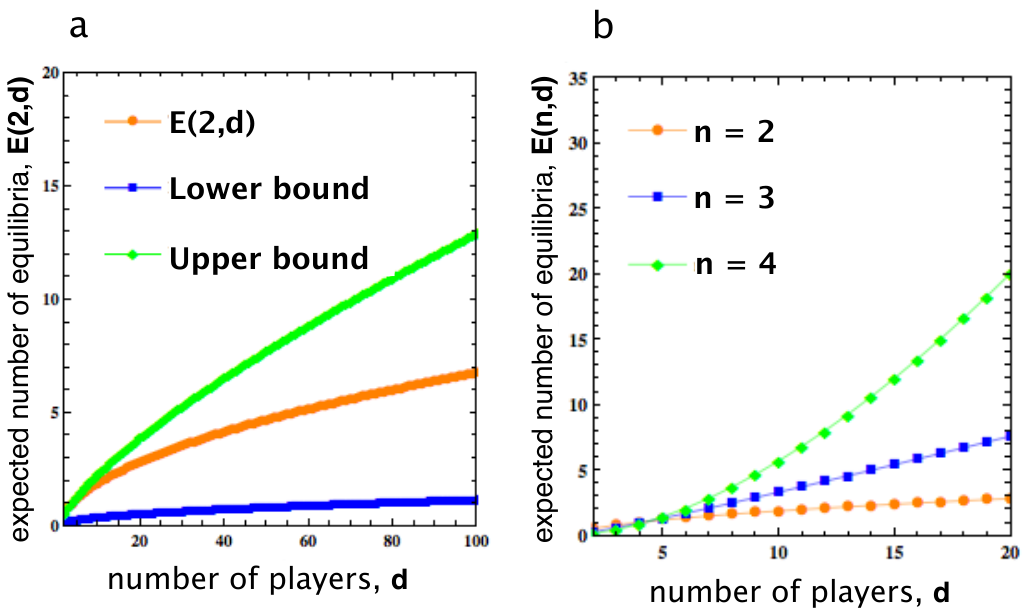
In Figure 1a, we show the numerical results for $E(2,d)$ in comparison with the obtained upper and lower bounds.

Corollary 1

1)

The expected number of equilibria increases unboundedly when $d$ tends to infinity

$\lim_{d\rightarrow\infty}E(2,d)=+\infty.$ (34)
2)

The probability $p_{m}$ of observing $m$ equilibria, $1\leq m\leq d-1$ , is bounded by

$p_{m}\leq\frac{E(2,d)}{m}\leq\frac{1}{\pi m}\sqrt{d-1}\sqrt{1+\frac{\pi}{2}\sqrt{d-1}}.$ (35)

In particular,

$p_{d-1}\leq\frac{1}{\pi}\frac{\sqrt{1+\frac{\pi}{2}\sqrt{d-1}}}{\sqrt{d-1}},\quad\text{and}\quad\lim_{d\rightarrow\infty}p_{d-1}=0.$

Proof

1)

This is a direct consequence of (29), as the lower bound of $E(2,d)$ tends to infinity when $d$ tends to infinity.
2)

This is again a direct consequence of (29) and definition of $E(2,d)$ . For any $1\leq m\leq d-1$ , we have

$E(2,d)=\sum_{i=1}^{d-1}p_{i}\cdot i\geq p_{m}\cdot m.$

In particular,

$p_{d-1}\leq\frac{E(2,d)}{d-1}\leq\frac{1}{\pi}\frac{\sqrt{1+\frac{\pi}{2}\sqrt{d-1}}}{\sqrt{d-1}}.$

As a consequence, $\lim\limits_{d\rightarrow\infty}p_{d-1}=0$ . More generally, we can see that this limit is true for $p_{k}$ for any $k=O(d)$ as $d\rightarrow\infty$ .

From this corollary we can see that, interestingly, although the mean number of equilibria tends to infinity when the number of players $d$ increases, the probability to see the maximal number of equilibria in a $d$ -player system converges to 0. There has been extensive research studying the maximal number of equilibrium points of a dynamical system MS (82); Kar (80); VC88a (); VC88b (); KF (70); VC88c (); BCV (93); BCV (97); Alt (10). Our results suggest that the possibility to reach such a maximal number is very small when $d$ is sufficiently large.

Corollary 2

The expected number of stable equilibrium points in a random game with $d$ players and two strategies is equal to $\frac{E(2,d)}{2}$ , and is thus bounded within to the following interval

\left[\frac{d-1}{2\pi\sqrt{2d-3}},\ \frac{1}{2\pi}\sqrt{d-1}\sqrt{1+\frac{\pi}{2}\sqrt{d-1}}\right].

Proof

From (HTG, 12, Theorem 3), it is known that an equilibrium in a random game with two strategies and an arbitrary number of players, is stable with probability $1/2$ . Hence, the corollary is a direct consequence of Theorem 3.1.

3.2 Two-player multi-strategy games

In this section, we consider games with two players, i.e. $d=2$ , and arbitrary strategies. In this case (7) is simplified to a linear system

\begin{cases}\sum_{j}\beta^{i}_{j}\,y_{j}=0,\quad\text{for}~~i=1,\ldots,n-1,\\ \sum_{j}y_{j}=1,\end{cases}

(36)

where $\beta_{j}^{i}$ have Gaussian distributions with mean $0$ and variance $1$ . The main result of this section is the following explicit formula for $E(n,2)$ .

Theorem 3.2

We have

E(n,2)=\frac{1}{2^{n-1}}.

(37)

This theorem can be seen as a direct application of (HTG, 12, Theorem 1) and the definition of $E(n,d)$ in Eq. (14). Indeed, according to (HTG, 12, Theorem 1), the probability that Eq. (36) has a (unique) isolated solution is $p_{1}=2^{1-n}$ and the probability of having no solution is $0$ . By (14), $E(n,2)=p_{1}$ , and hence $E(n,2)=2^{1-n}$ .

To demonstrate further the usefulness of our approach using the random polynomial theory, we present here an alternative proof that can directly obtain $E(n,2)$ , i.e. without computing the probability of observing concrete numbers of equilibria. Our proof requires an assumption that $\{A^{i}=(\beta_{j}^{i})_{j=1,\cdots,n-1};i=1,\ldots,n-1\}$ are independent random vectors. We will elaborate and discuss this assumption in Remark 4. The main ingredient of our proof is the following lemma, whose proof is given in Appendix 5.4.

Lemma 3

Let $t_{1},\dots,t_{n-1}$ be real numbers, and let $L$ be the matrix with entries

		$\displaystyle L_{ii}=\frac{1}{1+\sum\limits_{k=1}^{n-1}t_{k}^{2}}-\frac{t_{i}^{2}}{(1+\sum\limits_{k=1}^{n-1}t_{k}^{2})^{2}},$
		$\displaystyle L_{ij}=\frac{-t_{i}t_{j}}{(1+\sum\limits_{k=1}^{n-1}t_{k}^{2})^{2}}\quad\forall i\neq j.$

It holds that

\det L=\frac{1}{\left(1+\sum\limits_{k=1}^{n-1}t_{k}^{2}\right)^{n}}.

(38)

Proof (Proof of Theorem 3.2 under the assumption that $\{A^{i}=(\beta_{j}^{i})_{j=1,\cdots,n-1};i=1,\ldots,n-1\}$ are independent random vectors.)

Let $L$ be the matrix in Lemma 3. According to Lemma 1 and Lemma 3, we have

	$\displaystyle E(n,2)$	$\displaystyle=\pi^{-\frac{n}{2}}\Gamma\left(\frac{n}{2}\right)\underbrace{\int_{0}^{\infty}\ldots\int_{0}^{\infty}}_{n-1\,\text{times}}\left(\det L\right)^{1/2}\,dt_{1}\ldots dt_{n-1}$
		$\displaystyle=\pi^{-\frac{n}{2}}\Gamma\left(\frac{n}{2}\right)\underbrace{\int_{0}^{\infty}\ldots\int_{0}^{\infty}}_{n-1\,\text{times}}\left(1+\sum_{k=1}^{n-1}t_{k}^{2}\right)^{-n/2}\,dt_{1}\ldots dt_{n-1}$
		$\displaystyle=\frac{1}{2}\pi^{-\frac{n-1}{2}}\Gamma\left(\frac{n-1}{2}\right)\underbrace{\int_{0}^{\infty}\ldots\int_{0}^{\infty}}_{n-2\,\text{times}}\left(1+\sum_{k=1}^{n-2}t_{k}^{2}\right)^{-(n-1)/2}\,dt_{1}\ldots dt_{n-2}$
		$\displaystyle\ldots$
		$\displaystyle=\frac{1}{2^{n-1}}\pi^{-\frac{1}{2}}\Gamma\left(\frac{1}{2}\right)$
		$\displaystyle=\frac{1}{2^{n-1}},$

where we have repeatedly used the equality (with $a>0$ and $p>1$ )

\int_{0}^{\infty}(a+t^{2})^{-p}dt=\frac{\sqrt{\pi}\ \Gamma{(p-\frac{1}{2})}}{2\ \Gamma(p)}a^{\frac{1}{2}-p}.

Remark 3

Note that, as in (HTG, 12, Theorem 2), it is known that the probability that a two-player $n$ -strategy random game has a stable (internal) equilibrium is at most $2^{-n}$ . Hence, the expected number of stable equilibrium points in this case is at most $2^{-n}$ . From (HTG, 12, Theorem 2), we also can show that this bound is sharp only when $n=2$ .

Remark 4

Let $M$ be the number of sequences $(k_{1},\ldots,k_{n-1})$ such that $\sum_{j=1}^{n-1}k_{j}\leq d-1$ . For each $i=1,\ldots,n-1$ , we define a random vector $A^{i}=(\beta^{i}_{k_{1},\ldots,k_{n-1}})\in\mathbb{R}^{M}$ . Recalling from Section 2 that $\beta^{i}_{k_{1},...,k_{n-1}}=\alpha^{i}_{k_{1},...,k_{n}}-\alpha^{n}_{k_{1},...,k_{n}}$ , where $\alpha^{i}_{i_{1},\ldots,i_{d-1}}$ is the payoff of the focal player, with $i$ ( $1\leq i\leq n$ ) being the strategy of the focal player, and $i_{k}$ (with $1\leq i_{k}\leq n$ and $1\leq k\leq d-1$ ) is the strategy of the player in position $k$ . The assumption in Lemma 1 is that $A^{1},\ldots,A^{n-1}$ are independent random vectors and each of them has mean $0$ and covariance matrix $C$ . This assumption clearly holds for $n=2$ . For $n>2$ , the assumption holds only under quite restrictive conditions such as $\alpha^{n}_{k_{1},...,k_{n}}$ is deterministic or $\alpha^{i}_{k_{1},...,k_{n}}$ are essentially identical. Nevertheless, from a purely mathematical point of view (see for instance Kos (93); Kos (02) and Section 4 for further discussion), it is important to investigate the number of real zeros of the system (7) under the assumption of independence of $\{A^{i}\}$ since this system has not been studied in the literature. As such, the investigation provides new insights into the theory of zeros of systems of random polynomials. In addition, it also gives important hint on the complexity of the game theoretical question, i.e. the number of expected number of equilibria. Indeed, for $d=2$ and arbitrary $n$ , the assumption does not affect the final result as shown in Theorem 3.2. We recall that (EK, 95, Theorem 7.1) also required that the rows $\{A^{i}\}$ are independent random vectors. Hence to treat the general case, one would need to generalize (EK, 95, Theorem 7.1) and this is a difficult problem as demonstrated in Kos (93); Kos (02). With this motivation, in the next section, we keep the assumption of independence of $\{A^{i}\}$ and leave the general case for future research. We numerically compute the number of zeros of the system (7) for $n\in\{2,3,4\}$ . Again, as we shall see, the numerical results under the given assumption lead to outcomes closely corroborated by previous works in GT (10); HTG (12).

3.3 Multi-player multi-strategy games

We now move to the general case of multi-player games with multiple strategies. We provide numerical results for this case. For simplicity of notation in this section we write $\sum\limits_{k_{1},\ldots,k_{n-1}}$ instead of $\sum\limits_{\begin{subarray}{c}0\leq k_{1},...,k_{n-1}\leq d-1,\\ \sum^{n-1}_{i=1}k_{i}\leq d-1\end{subarray}}$ and $\sum\limits_{k_{1},\ldots,k_{n-1}|k_{i_{1}},..,k_{i_{m}}}$ instead of $\sum\limits_{\begin{subarray}{c}0\leq k_{i}\leq d-1\ \forall i\in S\setminus R,\\ 1\leq k_{j}\leq d-1\ \forall j\in R,\\ \sum^{n-1}\limits_{i=1}k_{i}\leq d-1\end{subarray}}$ where $S=\{1,\ldots,n-1\}$ and $R=\{i_{1},\ldots,i_{m}\}\subseteq S$ .

According to Lemma 1, the expected number of internal equilibria in a $d-$ player random game with $n$ strategies is given by

	$\displaystyle E(n,d)$	$\displaystyle=\pi^{-\frac{n}{2}}\Gamma\left(\frac{n}{2}\right)\int_{U}\left(\det\left[\frac{\partial^{2}}{\partial x_{i}y_{j}}(\log v(x)^{T}Cv(y))\big\|_{y=x=t}\right]_{ij}\right)^{\frac{1}{2}}dt$
		$\displaystyle=\pi^{-\frac{n}{2}}\Gamma\left(\frac{n}{2}\right)\int_{U}\left(\det L\right)^{\frac{1}{2}}dt,$

where $\Gamma$ is the Gamma function, and $L$ denotes the matrix with entries

\displaystyle L_{ij}

\displaystyle=\frac{\partial^{2}}{\partial x_{i}y_{j}}(\log v(x)^{T}Cv(y))\big|_{y=x=t}.

We have

v(x)^{T}Cv(y)=\sum\limits_{k_{1},\ldots,k_{n-1}}\begin{pmatrix}d-1\\ k_{1},\ldots,k_{n}\end{pmatrix}^{2}\prod\limits_{i=1}^{n}x_{i}^{k_{i}}y_{i}^{k_{i}}.

Set $\Pi(x,y):=\prod\limits_{l=1}^{n-1}x_{l}^{k_{l}}y_{l}^{k_{l}}$ . Then

		$\displaystyle\frac{\partial^{2}}{\partial x_{i}y_{j}}(\log v(x)^{T}Cv(y))$
		$\displaystyle\quad=\frac{\frac{1}{x_{i}y_{j}}\sum\limits_{k_{1},...,k_{n-1}\|k_{i},k_{j}}k_{i}k_{j}\begin{pmatrix}d-1\\ k_{1},\ldots,k_{n-1}\end{pmatrix}^{2}\Pi(x,y)}{\sum\limits_{k_{1},\ldots,k_{n-1}}\begin{pmatrix}d-1\\ k_{1},\ldots,k_{n-1}\end{pmatrix}^{2}\Pi(x,y)}$
		$\displaystyle\qquad-\frac{\left(\frac{1}{x_{i}}\sum\limits_{k_{1},\ldots,k_{n-1}\|k_{i}}k_{i}\begin{pmatrix}d-1\\ k_{1},\ldots,k_{n}\end{pmatrix}^{2}\Pi(x,y)\right)\left(\frac{1}{y_{j}}\sum\limits_{k_{1},...,k_{n}\|k_{j}}k_{j}\begin{pmatrix}d-1\\ k_{1},\ldots,k_{n}\end{pmatrix}^{2}\Pi(x,y)\right)}{\left(\sum\limits_{k_{1},\ldots,k_{n-1}}\begin{pmatrix}d-1\\ k_{1},\ldots,k_{n}\end{pmatrix}^{2}\Pi(x,y)\right)^{2}}.$

Therefore

	$\displaystyle L_{ij}$	$\displaystyle=\frac{\frac{1}{t_{i}t_{j}}\sum\limits_{k_{1},\ldots,k_{n-1}\|k_{i},k_{j}}k_{i}k_{j}\begin{pmatrix}d-1\\ k_{1},\ldots,k_{n}\end{pmatrix}^{2}\prod\limits_{l}t_{l}^{2k_{l}}}{\sum\limits_{k_{1},\ldots,k_{n-1}}\begin{pmatrix}d-1\\ k_{1},\ldots,k_{n}\end{pmatrix}^{2}\prod\limits_{l}t_{l}^{2k_{l}}}$		(39)
		$\displaystyle\qquad-\frac{\left(\frac{1}{t_{i}}\sum\limits_{k_{1},...,k_{n-1}\|k_{i}}k_{i}\begin{pmatrix}d-1\\ k_{1},\ldots,k_{n}\end{pmatrix}^{2}\prod\limits_{l}t_{l}^{2k_{l}}\right)\left(\frac{1}{t_{j}}\sum\limits_{k_{1},...,k_{n-1}\|k_{j}}k_{j}\begin{pmatrix}d-1\\ k_{1},\ldots,k_{n}\end{pmatrix}^{2}\prod\limits_{l}t_{l}^{2k_{l}}\right)}{\left(\sum\limits_{k_{1},\ldots,k_{n-1}}\begin{pmatrix}d-1\\ k_{1},\ldots,k_{n}\end{pmatrix}^{2}\prod\limits_{l}t_{l}^{2k_{l}}\right)^{2}}.$		(40)

So far in the paper we have assumed that all the $\beta^{i}_{k_{1},...,k_{n-1}}$ in Eq. (7) are standard normal distributions. The following lemma shows, as a consequence of the above described formula, that all the results obtained so far remain valid if they have a normal distribution with mean zero and arbitrary variance (i.e. the entries of the game payoff matrix have the same, arbitrary normal distribution).

Lemma 4

Suppose $\beta^{i}_{k_{1},...,k_{n-1}}$ have normal distributions with mean 0 and arbitrary variance $\sigma^{2}$ . Then, $L_{ij}$ as defined in (39) does not depend on $\sigma^{2}$ .

Proof

In this case, $\beta^{i}_{k_{1},...,k_{n-1}}\begin{pmatrix}d-1\\ k\end{pmatrix}$ has a Gaussian distribution with variance $\sigma^{2}\begin{pmatrix}d-1\\ k\end{pmatrix}^{2}$ and mean $0$ . Hence,

v(x)^{T}Cv(y)=\sum\limits_{k_{1},\ldots,k_{n-1}}\sigma^{2}\begin{pmatrix}d-1\\ k_{1},\ldots,k_{n}\end{pmatrix}^{2}\prod\limits_{i=1}^{n}x_{i}^{k_{i}}y_{i}^{k_{i}}.

Repeating the same calculation we obtain the same $L_{ij}$ as in (39), which is independent of $\sigma$ .

This result suggests that when dealing with random games as in this article, it is sufficient to consider that payoff entries are from the interval $[0,1]$ instead of from an arbitrary one, as done numerically in GT (10). A similar behaviour has been observed in HTG (12) for the analysis and computation with small $d$ or $n$ , showing that results are not dependent on the interval where the payoff entries are drawn. Furthermore, it is noteworthy that this result confirms the observation that multiplying a payoff matrix by a constant does not change the equilibria HS (98), provided a one-to-one mapping from [0,1] to the arbitrary interval.

Example 2 (d-players with n=3 strategies)

	$\displaystyle L_{11}$	$\displaystyle=\frac{\frac{1}{t_{1}^{2}}\sum\limits_{k_{1}=1,k_{2}=0}k_{1}^{2}\begin{pmatrix}d-1\\ k_{1},k_{2}\end{pmatrix}^{2}t_{1}^{2k_{1}}t_{2}^{2k_{2}}}{\sum\limits_{k_{1},k_{2}}\begin{pmatrix}d-1\\ k_{1},k_{2}\end{pmatrix}^{2}t_{1}^{2k_{1}}t_{2}^{2k_{2}}}-\frac{\left(\frac{1}{t_{1}}\sum\limits_{k_{1}=1,k_{2}=0}k_{1}\begin{pmatrix}d-1\\ k_{1},k_{2}\end{pmatrix}^{2}t_{1}^{2k_{1}}t_{2}^{2k_{2}}\right)^{2}}{\left(\sum\limits_{k_{1},k_{2}}\begin{pmatrix}d-1\\ k_{1},k_{2}\end{pmatrix}^{2}t_{1}^{2k_{1}}t_{2}^{2k_{2}}\right)^{2}},$
	$\displaystyle L_{12}$	$\displaystyle=\frac{\frac{1}{t_{1}t_{2}}\sum\limits_{k_{1}=1,k_{2}=1}k_{1}k_{2}\begin{pmatrix}d-1\\ k_{1},k_{2}\end{pmatrix}^{2}t_{1}^{2k_{1}}t_{2}^{2k_{2}}}{\sum\limits_{k_{1},k_{2}}\begin{pmatrix}d-1\\ k_{1},k_{2}\end{pmatrix}^{2}t_{1}^{2k_{1}}t_{2}^{2k_{2}}}$
		$\displaystyle\qquad-\frac{\left(\frac{1}{t_{1}}\sum\limits_{k_{1}=1,k_{2}=0}k_{1}\begin{pmatrix}d-1\\ k_{1},k_{2}\end{pmatrix}^{2}t_{1}^{2k_{1}}t_{2}^{2k_{2}}\right)\left(\frac{1}{t_{2}}\sum\limits_{k_{1}=0,k_{2}=1}k_{2}\begin{pmatrix}d-1\\ k_{1},k_{2}\end{pmatrix}^{2}t_{1}^{2k_{1}}t_{2}^{2k_{2}}\right)}{\left(\sum\limits_{k_{1},k_{2}}\begin{pmatrix}d-1\\ k_{1},k_{2}\end{pmatrix}^{2}t_{1}^{2k_{1}}t_{2}^{2k_{2}}\right)^{2}},$
	$\displaystyle L_{21}$	$\displaystyle=L_{12},$
	$\displaystyle L_{22}$	$\displaystyle=\frac{\frac{1}{t_{2}^{2}}\sum\limits_{k_{1}=0,k_{2}=1}k_{2}^{2}\begin{pmatrix}d-1\\ k_{1},k_{2}\end{pmatrix}^{2}t_{1}^{2k_{1}}t_{2}^{2k_{2}}}{\sum\limits_{k_{1},k_{2}}\begin{pmatrix}d-1\\ k_{1},k_{2}\end{pmatrix}^{2}t_{1}^{2k_{1}}t_{2}^{2k_{2}}}-\frac{\left(\frac{1}{t_{2}}\sum\limits_{k_{1}=0,k_{2}=1}k_{2}\begin{pmatrix}d-1\\ k_{1},k_{2}\end{pmatrix}^{2}t_{1}^{2k_{1}}t_{2}^{2k_{2}}\right)^{2}}{\left(\sum\limits_{k_{1},k_{2}}\begin{pmatrix}d-1\\ k_{1},k_{2}\end{pmatrix}^{2}t_{1}^{2k_{1}}t_{2}^{2k_{2}}\right)^{2}}.$

Therefore,

E(3,d)=\pi^{-\frac{3}{2}}\Gamma\left(\frac{3}{2}\right)\int_{0}^{\infty}\int_{0}^{\infty}\sqrt{L_{11}L_{22}-L_{12}L_{21}}\,dt_{1}dt_{2}.

Next we provide some numerical results. We numerically compute $E(n,d)$ for $n\in\{2,3,4\}$ , and show them in Table 1 (for $d\leq 10$ ) and Figure 1b (for $d\leq 20$ ). We also plot the lower and upper bounds for $E(2,d)$ obtained in Theorem 3.1 and compare them with its numerical computation, see Figure 1a. We note that for small $n$ and $d$ (namely, $n\leq 5$ and $d\leq 4$ ), $E(n,d)$ can also be computed numerically via the probabilities $p_{i}$ of observing exactly $i$ equilibria using (14). This direct approach has been used in HTG (12) and GT (10), which our results are compatible with. Furthermore, as a consequence of Corollary 2, we can derive the exact expected number of stable equilibria for $n=2$ , which is equal to half of the expected number of equilibria given in the first row of Table 1.

Table 1: Expected number of internal equilibria for some values of

d

and

n

d	2	3	4	5	6	7	8	9	10
$n=2$	0.5	0.77	0.98	1.16	1.31	1.47	1.60	1.73	1.84
$n=3$	0.25	0.57	0.92	1.29	1.67	2.06	2.46	2.86	3.27
$n=4$	0.125	0.41	0.84	1.39	2.05	2.81	3.67	4.62	5.66

Refer to caption — Figure 1: (a) Expected number of equilibria, $E(2,d)$ , for varying the number of players in the game, and the upper and lower bounds obtained in Theorem 3.1. (b) Expected number of equilibria, $E(n,d)$ , for varying the number of players and strategies in the game. We plot for different number of strategies: $n=2$ , 3 and 4. The payoff entries of the d-player n-strategy game are randomly drawn from the normal distribution. In general, the larger the number of players in the game, the higher the number of equilibria one can expect if the payoff entries of the game are randomly chosen. We observe that for small $d$ , $E(n,d)$ increases with $n$ while it decreases for large $d$ (namely, $d\geq 5$ , see also Table 1). The results were obtained numerically using Mathematica.

4 Discussion

In the evolutionary game literature, mathematical results have been mostly provided for two-player games HS (98); Now (06), despite the abundance of multi-player game examples in nature BCV (97); GT (10). The mathematical study for multi-player games has only attracted more attention recently, apparently because the resulting complexity and dynamics from the games are significantly magnified with the number of the game participants BCV (97); HTG (12); WTG (13). As seen from our analysis, multi-player games introduce non-linearity into the inducing equations, because the fitness functions are polynomial instead of linear as in the pairwise interactions HS (98); GT (10); WTG (13). It is even more so if we consider scenarios in which the payoff matrix is non-linear naturally, such as for public goods games with non-linear returns PSSS (09), as observed in animals hunting Sta (92); PC (97). In addition, as the number of strategies increases, one needs to deal with systems of multivariate polynomials. This seemingly complexity of the general multi-player multi-strategy games makes the analysis of the equilibrium points extremely difficult. For instance, in HTG (12), as the analysis was based on an explicit calculation of the zeros of systems of polynomials, it cannot go beyond games with a small number of players (namely, $d\leq 5$ ), even for the simplest case of $n=2$ . Here we have taken a different approach based on the well-established theory of random polynomials. We have derived a computationally implementable formula, $E(n,d)$ , of the mean number of equilibria in a general random $d$ -player game with $n$ strategies. For $n=2$ and with an arbitrary $d$ , we have derived asymptotic upper and lower bounds of $E(2,d)$ . An interesting implication of these results is that although the expected number of equilibria tends to infinity when $d$ increases, the probability of seeing the maximal possible number of equilibria tends to 0. This is a notable observation since knowing the maximal number of equilibrium points in an evolutionary process is insightful and has been of special focus in biological contexts Lev (00); GT (10). Furthermore, for $d=2$ with an arbitrary $n$ , we have derived the exact value $E(n,2)=2^{1-n}$ , recovering results obtained in HTG (12). In the general case, based on the formula that we have derived, we have been able to numerically calculate $E(n,d)$ , thereby going beyond the analytical and numerical computations from previous work that made use of the direct approach. As a consequence of the results obtained for the extreme cases, we could also derive the boundaries for the expected number of equilibrium points when counting only the stable ones. Note that some studies have been carried out to study the stable equilibrium points or evolutionary stable strategies (ESS) MS (82) in a random evolutionary game, but it has been mostly done for two-player games, see for example Hai (88); KS (09); HRW (08). As such, we have provided further understanding with respect to the asymptotic behaviour of the expected number of stable equilibria for multi-player random games, though with only two strategies, leaving the more general case for future study.

On the other hand, in the random polynomial literature, the study of distribution of zeros of system of random polynomials as described in (8), especially in the univariate case, has been carried out by many authors, see for instance EK (95) for a nice exposition and TV (14) for the most recent results. The most well-known classes of polynomials are: flat polynomials or Weyl polynomials for $a_{i}\mathrel{\mathchoice{\vbox{\hbox{$\displaystyle:$}}}{\vbox{\hbox{$\textstyle:$}}}{\vbox{\hbox{$\scriptstyle:$}}}{\vbox{\hbox{$\scriptscriptstyle:$}}}{=}}\frac{1}{i!}$ , elliptic polynomials or binomial polynomials for $a_{i}\mathrel{\mathchoice{\vbox{\hbox{$\displaystyle:$}}}{\vbox{\hbox{$\textstyle:$}}}{\vbox{\hbox{$\scriptstyle:$}}}{\vbox{\hbox{$\scriptscriptstyle:$}}}{=}}\sqrt{\begin{pmatrix}d-1\\ i\end{pmatrix}}$ and Kac polynomials for $a_{i}\mathrel{\mathchoice{\vbox{\hbox{$\displaystyle:$}}}{\vbox{\hbox{$\textstyle:$}}}{\vbox{\hbox{$\scriptstyle:$}}}{\vbox{\hbox{$\scriptscriptstyle:$}}}{=}}1$ . We emphasize the difference between the polynomial studied in this paper with the elliptic case: $a_{i}=\begin{pmatrix}d-1\\ i\end{pmatrix}$ are binomial coefficients, not their square root. In the elliptic case, $v(x)^{T}Cv(y)=\sum_{i=1}^{d-1}\begin{pmatrix}d-1\\ i\end{pmatrix}x^{i}y^{i}=(1+xy)^{d-1}$ , and as a result $E=E(2,d)=\sqrt{d-1}$ . While in our case, because of the square in the coefficients, $v(x)^{T}Cv(y)=\sum_{i=1}^{d-1}\begin{pmatrix}d-1\\ i\end{pmatrix}^{2}x^{i}y^{i}$ is no longer a generating function. Whether one can find an exact formula for $E(2,d)$ is unclear. For the multivariate situation, the exact formula for $E(n,2)$ is interesting by itself and we could not be able to find it in the literature. Due to the complexity in the general case $d,n\geq 3$ , further research is required.

In short, we have described a novel approach to calculating and analyzing the expected number of (stable) equilibrium points in a general random evolutionary game, giving insights into the overall complexity of such dynamical systems as the players and the strategies in the game increase. Since the theory of random polynomials is rich, we envisage that our method could be extended to obtain results for other more complex scenarios such as games having a payoff matrix with dependent entries and/or with general distributions.

5 Appendix

5.1 Properties of $a_{k}$

In the following we prove that $a_{2d-4-k}=a_{k}$ for all $0\leq k\leq 2d-4$ , i.e. (22). First, we transform $a_{k}$ as follows

	$\displaystyle a_{k}$	$\displaystyle=\sum\limits_{\begin{subarray}{c}0\leq i\leq d-1\\ 0\leq j\leq d-2\\ i+j=k\end{subarray}}\begin{pmatrix}d-1\\ i\end{pmatrix}^{2}\begin{pmatrix}d-2\\ j\end{pmatrix}^{2}-\sum\limits_{\begin{subarray}{c}0\leq i^{\prime}\leq d-2\\ 0\leq j^{\prime}\leq d-2\\ i^{\prime}+j^{\prime}=k-1\end{subarray}}\begin{pmatrix}d-2\\ i^{\prime}\end{pmatrix}\begin{pmatrix}d-1\\ i^{\prime}+1\end{pmatrix}\begin{pmatrix}d-2\\ j^{\prime}\end{pmatrix}\begin{pmatrix}d-1\\ j^{\prime}+1\end{pmatrix}$
		$\displaystyle=\begin{pmatrix}d-2\\ k\end{pmatrix}^{2}+\sum\limits_{\begin{subarray}{c}0\leq i\leq d-2\\ 0\leq j\leq d-2\\ i+j=k-1\end{subarray}}\begin{pmatrix}d-1\\ i+1\end{pmatrix}^{2}\begin{pmatrix}d-2\\ j\end{pmatrix}^{2}-\sum\limits_{\begin{subarray}{c}0\leq i^{\prime}\leq d-2\\ 0\leq j^{\prime}\leq d-2\\ i^{\prime}+j^{\prime}=k-1\end{subarray}}\begin{pmatrix}d-2\\ i^{\prime}\end{pmatrix}\begin{pmatrix}d-1\\ i^{\prime}+1\end{pmatrix}\begin{pmatrix}d-2\\ j^{\prime}\end{pmatrix}\begin{pmatrix}d-1\\ j^{\prime}+1\end{pmatrix}$
		$\displaystyle=\begin{pmatrix}d-2\\ k\end{pmatrix}^{2}+\sum\limits_{\begin{subarray}{c}0\leq i\leq d-2\\ 0\leq j\leq d-2\\ i+j=k-1\end{subarray}}\begin{pmatrix}d-1\\ i+1\end{pmatrix}\begin{pmatrix}d-2\\ j\end{pmatrix}\left(\begin{pmatrix}d-1\\ i+1\end{pmatrix}\begin{pmatrix}d-2\\ j\end{pmatrix}-\begin{pmatrix}d-2\\ i\end{pmatrix}\begin{pmatrix}d-1\\ j+1\end{pmatrix}\right)$
		$\displaystyle=\begin{pmatrix}d-2\\ k\end{pmatrix}^{2}+\sum\limits_{\begin{subarray}{c}0\leq i\leq j\leq d-2\\ i+j=k-1\end{subarray}}\left(\begin{pmatrix}d-1\\ i+1\end{pmatrix}\begin{pmatrix}d-2\\ j\end{pmatrix}-\begin{pmatrix}d-2\\ i\end{pmatrix}\begin{pmatrix}d-1\\ j+1\end{pmatrix}\right)^{2}$

Now we prove that $a_{2d-4-k}=a_{k}$ . Indeed, we have

	$\displaystyle a_{2d-4-k}$	$\displaystyle=\begin{pmatrix}d-2\\ 2d-4-k\end{pmatrix}^{2}+\sum\limits_{\begin{subarray}{c}0\leq i\leq j\leq d-2\\ i+j=2d-k-5\end{subarray}}\left(\begin{pmatrix}d-2\\ i+1\end{pmatrix}\begin{pmatrix}d-2\\ j\end{pmatrix}-\begin{pmatrix}d-2\\ i\end{pmatrix}\begin{pmatrix}d-1\\ j+1\end{pmatrix}\right)^{2}$
		(we use here the transformations $i=d-3-i$ and $j=d-3-j$ )
		$\displaystyle=\begin{pmatrix}d-2\\ 2d-4-k\end{pmatrix}^{2}+\sum\limits_{\begin{subarray}{c}-1\leq j\leq i\leq d-3\\ i+j=k-1\end{subarray}}\left(\begin{pmatrix}d-1\\ i+1\end{pmatrix}\begin{pmatrix}d-2\\ j+1\end{pmatrix}-\begin{pmatrix}d-2\\ i+1\end{pmatrix}\begin{pmatrix}d-1\\ j+1\end{pmatrix}\right)^{2}$
		$\displaystyle=\begin{pmatrix}d-2\\ 2d-4-k\end{pmatrix}^{2}+\sum\limits_{\begin{subarray}{c}-1\leq j\leq i\leq d-3\\ i+j=k-1\end{subarray}}\left(\begin{pmatrix}d-1\\ i+1\end{pmatrix}\begin{pmatrix}d-2\\ j\end{pmatrix}-\begin{pmatrix}d-2\\ i\end{pmatrix}\begin{pmatrix}d-1\\ j+1\end{pmatrix}\right)^{2}.$

Since for $j=-1$ and $i=k$ we have

\left(\begin{pmatrix}d-1\\ i+1\end{pmatrix}\begin{pmatrix}d-2\\ j\end{pmatrix}-\begin{pmatrix}d-2\\ i\end{pmatrix}\begin{pmatrix}d-1\\ j+1\end{pmatrix}\right)^{2}=\begin{pmatrix}d-1\\ k\end{pmatrix}^{2},

and for $j=d-2$ and $i=k-1-(d-2)$ , we have

	$\displaystyle\left(\begin{pmatrix}d-1\\ i+1\end{pmatrix}\begin{pmatrix}d-2\\ j\end{pmatrix}-\begin{pmatrix}d-2\\ i\end{pmatrix}\begin{pmatrix}d-1\\ j+1\end{pmatrix}\right)^{2}$	$\displaystyle=\left(\begin{pmatrix}d-1\\ k-(d-2)\end{pmatrix}-\begin{pmatrix}d-2\\ k-1-(d-2)\end{pmatrix}\right)^{2}$
		$\displaystyle=\begin{pmatrix}d-2\\ k-(d-2)\end{pmatrix}^{2}$
		$\displaystyle=\begin{pmatrix}d-2\\ 2d-4-k\end{pmatrix}^{2},$

it follows that $a_{2d-4-k}=a_{k}$ for all $0\leq k\leq 2d-4$ .

5.2 Detailed computation of $f(1)$

We use the following identities involving the square of binomial coefficients.

		$\displaystyle M_{d}(1)=\sum\limits_{k=0}^{d-1}\begin{pmatrix}d-1\\ k\end{pmatrix}^{2}=\begin{pmatrix}2(d-1)\\ d-1\end{pmatrix},$
		$\displaystyle A_{d}(1)=(d-1)^{2}M_{d-1}(1)=(d-1)^{2}\begin{pmatrix}2(d-2)\\ d-2\end{pmatrix},$
		$\displaystyle B_{d}(1)=\sum\limits_{k=1}^{d-1}k\begin{pmatrix}d-1\\ k\end{pmatrix}^{2}=\frac{d-1}{2}\begin{pmatrix}2(d-1)\\ d-1\end{pmatrix}.$

Therefore, we have

	$\displaystyle f(1)$	$\displaystyle=\frac{1}{\pi}\frac{\sqrt{A_{d}(1)M_{d}(1)-B_{d}(1)^{2}}}{M_{d}(1)}$
		$\displaystyle=\frac{1}{\pi}\frac{\sqrt{(d-1)^{2}\begin{pmatrix}2(d-1)\\ d-1\end{pmatrix}\left[\begin{pmatrix}2(d-2)\\ d-2\end{pmatrix}-\frac{1}{4}\begin{pmatrix}2(d-1)\\ d-1\end{pmatrix}\right]}}{\begin{pmatrix}2(d-1)\\ d-1\end{pmatrix}}$
		$\displaystyle=\frac{d-1}{\pi}\times\sqrt{\frac{\begin{pmatrix}2(d-2)\\ d-2\end{pmatrix}}{\begin{pmatrix}2(d-1)\\ d-1\end{pmatrix}}-\frac{1}{4}}$
		$\displaystyle=\frac{d-1}{\pi}\times\sqrt{\frac{d-1}{2(2d-3)}-\frac{1}{4}}$
		$\displaystyle=\frac{d-1}{2\pi\sqrt{2d-3}},$

where we have used the identity $\begin{pmatrix}2(n+1)\\ n+1\end{pmatrix}=\frac{n+1}{2(2n+1)}\begin{pmatrix}2n\\ n\end{pmatrix}.$

5.3 Alternative proof of the fifth property in Lemma 2

We show here an alternative proof of the fifth property without using the first one in Lemma 2.

Since $M_{d}\left(\frac{1}{t}\right)=t^{2(1-d)M_{d}(t)}$ , we have

	$\displaystyle M_{d}^{\prime}\left(\frac{1}{t}\right)$	$\displaystyle=-t^{3-2d}\left[2(1-d)M_{d}(t)+tM_{d}^{\prime}(t)\right],$
	$\displaystyle M_{d}^{\prime\prime}\left(\frac{1}{t}\right)$	$\displaystyle=t^{4-2d}\left[2(3-2d)(1-d)M_{d}(t)+2(3-2d)tM_{d}^{\prime}(t)+t^{2}M_{d}^{\prime\prime}(t)\right].$

Therefore, from (26), we have

B_{d}\left(\frac{1}{t}\right)=\frac{1}{2}M_{d}^{\prime}\left(\frac{1}{t}\right)=-t^{3-2d}\left[(1-d)M_{d}(t)+\frac{1}{2}tM_{d}^{\prime}(t)\right],

and

	$\displaystyle A_{d}\left(\frac{1}{t}\right)$	$\displaystyle=\frac{t}{4}\left[M_{d}^{\prime}\left(\frac{1}{t}\right)+\frac{1}{t}M_{d}^{\prime\prime}\left(\frac{1}{t}\right)\right]$
		$\displaystyle=\frac{1}{4}t^{4-2d}\left[4(1-d)^{2}+(5-4d)tM_{d}^{\prime}(t)+t^{2}M_{d}^{\prime\prime}(t)\right].$

Hence

	$\displaystyle A_{d}\left(\frac{1}{t}\right)M_{d}\left(\frac{1}{t}\right)-B_{d}\left(\frac{1}{t}\right)^{2}$	$\displaystyle=\frac{1}{4}t^{6-2d}\left[4(1-d)^{2}M_{d}(t)^{2}+(5-4d)tM_{d}^{\prime}(t)M_{d}(t)+t^{2}M_{d}^{\prime\prime}(t)M_{d}(t)\right]$
		$\displaystyle\qquad-t^{6-4d}\left[(1-d)M_{d}(t)+\frac{1}{2}tM_{d}^{\prime}(t)\right]^{2}$
		$\displaystyle=\frac{1}{4}t^{6-2d}\left[tM_{d}(t)M_{d}^{\prime}(t)+t^{2}M_{d}(t)M_{d}^{\prime\prime}(t)-t^{2}M_{d}^{\prime}(t)^{2}\right]$
		$\displaystyle=\frac{1}{4}t^{8-2d}\left[\frac{1}{t}M_{d}(t)M_{d}^{\prime}(t)+M_{d}(t)M_{d}^{\prime\prime}(t)-M_{d}^{\prime}(t)^{2}\right].$

Therefore,

	$\displaystyle f\left(\frac{1}{t}\right)$	$\displaystyle=\frac{1}{\pi}\frac{\sqrt{A_{d}\left(\frac{1}{t}\right)M_{d}\left(\frac{1}{t}\right)-B_{d}\left(\frac{1}{t}\right)^{2}}}{M_{d}\left(\frac{1}{t}\right)}$
		$\displaystyle=\frac{1}{\pi}\frac{t^{4-2d}\sqrt{\frac{1}{4t}\left[M_{d}(t)M_{d}^{\prime}(t)+tM_{d}(t)M_{d}^{\prime\prime}(t)-tM_{d}^{\prime}(t)^{2}\right]}}{t^{2-2d}M_{d}(t)}$
		$\displaystyle=t^{2}\frac{1}{\pi}\frac{\sqrt{\frac{1}{4t}\left[M_{d}(t)M_{d}^{\prime}(t)+tM_{d}(t)M_{d}^{\prime\prime}(t)-tM_{d}^{\prime}(t)^{2}\right]}}{M_{d}(t)}$
		$\displaystyle=t^{2}f(t).$

5.4 Proof of Lemma 3

Denoting $\Sigma=1+\sum_{k=1}^{n-1}t_{k}^{2}$ , we have

	$\displaystyle\det L$	$\displaystyle=\frac{1}{\Sigma^{2(n-1)}}\det\begin{pmatrix}\Sigma-t_{1}^{2}&-t_{1}t_{2}&\dots&-t_{1}t_{n-1}\\ -t_{2}t_{1}&\Sigma-t_{2}^{2}&\dots&-t_{2}t_{n-1}\\ \dots&\dots&\dots&\dots\\ -t_{n-1}t_{1}&-t_{n-1}t_{2}&\dots&\Sigma-t_{n-1}^{2}\end{pmatrix}$
		$\displaystyle=\frac{1}{t_{1}\dots t_{n-1}}\frac{1}{\Sigma^{2(n-1)}}\det\begin{pmatrix}t_{1}(\Sigma-t_{1}^{2})&-t_{1}t_{2}^{2}&\dots&-t_{1}t_{n-1}^{2}\\ -t_{2}t_{1}^{2}&t_{2}(\Sigma-t_{2}^{2})&\dots&-t_{2}t_{n-1}^{2}\\ \dots&\dots&\dots&\dots\\ -t_{n-1}t_{1}^{2}&-t_{n-1}t_{2}^{2}&\dots&t_{n-1}(\Sigma-t_{n-1}^{2})\end{pmatrix}$
		$\displaystyle=\frac{1}{t_{1}\dots t_{n-1}}\frac{1}{\Sigma^{2(n-1)}}\det\begin{pmatrix}t_{1}&-t_{1}t_{2}^{2}&\dots&-t_{1}t_{n-1}^{2}\\ t_{2}&t_{2}(\Sigma-t_{2}^{2})&\dots&-t_{2}t_{n-1}^{2}\\ \dots&\dots&\dots&\dots\\ t_{n-1}&-t_{n-1}t_{2}^{2}&\dots&t_{n-1}(\Sigma-t_{n-1}^{2})\end{pmatrix}$
		$\displaystyle=\frac{1}{\Sigma^{2(n-1)}}\det\begin{pmatrix}1&-t_{2}^{2}&\dots&-t_{n-1}^{2}\\ 1&\Sigma-t_{2}^{2}&\dots&-t_{n-1}^{2}\\ \dots&\dots&\dots&\dots\\ 1&-t_{2}^{2}&\dots&\Sigma-t_{n-1}^{2}\end{pmatrix}$
		$\displaystyle=\frac{1}{\Sigma^{2(n-1)}}\det\begin{pmatrix}1&-t_{2}^{2}&\dots&-t_{n-1}^{2}\\ 0&\Sigma&\dots&0\\ \dots&\dots&\dots&\dots\\ 0&0&\dots&\Sigma\end{pmatrix}$
		$\displaystyle=\frac{1}{\Sigma^{n}}.$

Acknowledgment

We would like to thank members of the WMS seminar at the CASA at Eindhoven University of Technology, especially Dr. R. van Hassel and Prof. A. Blokhuis for useful discussion. Part of this work was done under the support of the F.W.O. Belgium (TAH, postdoctoral fellowship 05_05 TR 7142).

References

[1] Niels Henrik Abel. Mémoire sur les équations algébriques, où l’on démontre l’impossibilité de la résolution de l’équation générale du cinquiéme degré. Abel’s Ouvres, (1):28–33, 1824.
[2] Lee Altenberg. Proof of the Feldman-Karlin conjecture on the maximum number of equilibria in an evolutionary system. Theoretical Population Biology, 77(4):263 – 269, 2010.
[3] M. Broom, C. Cannings, and G. T. Vickers. On the number of local maxima of a constrained quadratic form. Proc. R. Soc. Lond. A, 443:573–584, 1993.
[4] M Broom, C Cannings, and GT Vickers. Sequential methods for generating patterns of ess’s. Journal of Mathematical Biology, 32(6):597–615, 1994.
[5] M. Broom, C. Cannings, and G.T. Vickers. Multi-player matrix games. Bull. Math. Biol., 59(5):931–952, 1997.
[6] Mark Broom and Jan Rychtar. Game-theoretical models in biology. CRC Press, 2013.
[7] Alan Edelman and Eric Kostlan. How many zeros of a random polynomial are real? Bull. Amer. Math. Soc. (N.S.), 32(1):1–37, 1995.
[8] D. Fudenberg and C. Harris. Evolutionary dynamics with aggregate shocks. J. Econ. Theory, 57:420–441, 1992.
[9] Thilo Gross, Lars Rudolf, Simon A. Levin, and Ulf Dieckmann. Generalized models reveal stabilizing factors in food webs. Science, 325, 2009.
[10] Chaitanya S. Gokhale and Arne Traulsen. Evolutionary games in the multiverse. Proc. Natl. Acad. Sci. U.S.A., 107(12):5500–5504, 2010.
[11] John Haigh. The distribution of evolutionarily stable strategies. Journal of applied probability, pages 233–246, 1988.
[12] John Haigh. How large is the support of an ess? Journal of Applied Probability, pages 164–170, 1989.
[13] G. Hardin. The tragedy of the commons. Science, 162:1243–1248, 1968.
[14] C. Hauert, S. De Monte, J. Hofbauer, and K. Sigmund. Replicator dynamics for optional public good games. J. Theor. Biol., 218:187–194, 2002.
[15] The Anh Han, Luís Moniz Pereira, and Tom Lenaerts. Avoiding or Restricting Defectors in Public Goods Games? Journal of the Royal Society Interface, 2014 (In Press).
[16] Sergiu Hart, Yosef Rinott, and Benjamin Weiss. Evolutionarily stable strategies of random games, and the vertices of random polygons. The Annals of Applied Probability, pages 259–287, 2008.
[17] J. Hofbauer and K. Sigmund. Evolutionary Games and Population Dynamics. Cambridge University Press, Cambridge, 1998.
[18] The Anh Han, Arne Traulsen, and Chaitanya S. Gokhale. On equilibrium properties of evolutionary multi-player games with random payoff matrices. Theoretical Population Biology, 81(4):264 – 272, 2012.
[19] Samuel Karlin. The number of stable equilibria for the classical one-locus multiallele slection model. J. Math. Biology, 9:189–192, 1980.
[20] Samuel Karlin and Marcus W. Feldman. Linkage and selection: Two locus symmetric viability model. Theoretical Population Biology, 1:39–71, 1970.
[21] E. Kostlan. On the distribution of roots of random polynomials. In From Topology to Computation: Proceedings of the Smalefest (Berkeley, CA, 1990), pages 419–431. Springer, New York, 1993.
[22] E. Kostlan. On the expected number of real roots of a system of random polynomial equations. In Foundations of computational mathematics (Hong Kong, 2000), pages 149–188. World Sci. Publ., River Edge, NJ, 2002.
[23] Spyros C Kontogiannis and Paul G Spirakis. On the support size of stable strategies in random games. Theoretical Computer Science, 410(8):933–942, 2009.
[24] Simon A. Levin. Multiple scales and the maintenance of biodiversity. Ecosystems, 3:498–506, 2000.
[25] Andrew McLennan and Johannes Berg. Asymptotic expected number of nash equilibria of two-player normal form games. Games and Economic Behavior, 51(2):264–295, 2005.
[26] Andrew McLennan. The expected number of nash equilibria of a normal form game. Econometrica, 73(1):141–174, 2005.
[27] J. Maynard-Smith. Evolution and the Theory of Games. Cambridge University Press, Cambridge, 1982.
[28] M. A. Nowak. Evolutionary Dynamics. Harvard University Press, Cambridge, MA, 2006.
[29] C Packer and TM Caro. Foraging costs in social carnivores. Animal Behaviour, 54(5):1317–1318, 1997.
[30] Jorge M. Pacheco, Francisco C. Santos, Max O. Souza, and Brian Skyrms. Evolutionary dynamics of collective action in n-person stag hunt dilemmas. Proc. R. Soc. B, 276:315–321, 2009.
[31] K. Sigmund. The calculus of selfishness. Princeton Univ. Press, 2010.
[32] P. Schuster and K. Sigmund. Replicator dynamics. J. Theo. Biol., 100:533–538, 1983.
[33] F. C. Santos, M. D. Santos, and J. M. Pacheco. Social diversity promotes the emergence of cooperation in public goods games. Nature, 454:213–216, 2008.
[34] Philip E Stander. Cooperative hunting in lions: the role of the individual. Behavioral Ecology and Sociobiology, 29(6):445–454, 1992.
[35] P. D. Taylor and L. Jonker. Evolutionary stable strategies and game dynamics. Math. Biosci., 40:145–156, 1978.
[36] T. Tao and V. Vu. Local universality of zeroes of random polynomials. Int Math Res Notices, 2014.
[37] G. T. Vickers and C. Cannings. On the number of equilibria in a one-locus, multi allelic system. J. theor. Biol., 131:273–277, 1988.
[38] G. T. Vickers and C. Cannings. Patters of ESS’s I. J. theor. Biol., 132:387–408, 1988.
[39] G. T. Vickers and C. Cannings. Patters of ESS’s II. J. theor. Biol., 132:409–420, 1988.
[40] Bin Wu, Arne Traulsen, and Chaitanya S Gokhale. Dynamic properties of evolutionary multi-player games in finite populations. Games, 4(2):182–199, 2013.
[41] E. C. Zeeman. Population dynamics from game theory. in Lecture Notes in Mathematics, 819:471–497, 1980.

On the expected number of equilibria in a multi-player multi-strategy evolutionary game

Abstract

Keywords:

1 Introduction

2 Models and Methods

2.1 Evolutionary game theory and replicator dynamics

2.2 Random polynomial theory

Theorem 2.1

2.3 From random polynomial theory to evolutionary game theory

Lemma 1

3 Results

3.1 Multi-player two-strategy games

Lemma 2

Proof

Example 1

Proposition 1

Proof

Remark 1

Remark 2

Theorem 3.1

Proof

Corollary 1

Proof

Corollary 2

Proof

3.2 Two-player multi-strategy games

Theorem 3.2

Lemma 3

Proof (Proof of Theorem 3.2 under the assumption that {Ai=(βji)j=1,⋯,n−1;i=1,…,n−1}\{A^{i}=(\beta_{j}^{i})_{j=1,\cdots,n-1};i=1,\ldots,n-1\} are independent random vectors.)

Remark 3

Remark 4

3.3 Multi-player multi-strategy games

Lemma 4

Proof

Example 2 (d-players with n=3 strategies)

4 Discussion

5 Appendix

5.1 Properties of aka_{k}

5.2 Detailed computation of f⁡(1)f(1)

5.3 Alternative proof of the fifth property in Lemma 2

5.4 Proof of Lemma 3

Acknowledgment

References

Proof (Proof of Theorem 3.2 under the assumption that $\{A^{i}=(\beta_{j}^{i})_{j=1,\cdots,n-1};i=1,\ldots,n-1\}$ are independent random vectors.)

5.1 Properties of $a_{k}$

5.2 Detailed computation of $f(1)$