Volatility estimation under one-sided errors with applications to limit order books ^??

Consider observations $({\cal Y}_{i})$ above a stochastic boundary $(X_{t},\,t\in[0,1])$, which is formed by the graph of a continuous semi-martingale. The objective is to optimally recover the driving characteristic $\langle X,X\rangle_{t}$ of the boundary $X_{t}$, given the observations $({\cal Y}_{i})$. A quantification of the information content in these observations is non-trivial and leads to intriguing mathematical questions. One motivation for considering this stochastic boundary problem stems from financial applications in the context of limit order books. From a microeconomic point of view ask prices will typically lie above the efficient market price. Here the underlying latent efficient log-price of a stock $(X_{t},\,t\in[0,1])$, observed over a trading period like a day, serves as the boundary, whereas ask prices form the observations $({\cal Y}_{i})$. Bid prices can be handled symmetrically and independently, which can be used to validate the model.

Climate physics provides another example where semi-martingales appear as stochastic boundaries. Considerable efforts are devoted to understanding the driving stochastic term for SDEs modeling the long-term temperature evolution, see for instance [19] and [28]. One key source for historical temperature data is given by annual tree rings (dendrochronology and dendroclimatology, see e.g. [14]), whose relationship with temperature in an ideal environment is known. For individual trees only sizes up to this ideal boundary are observed due to growth obstructions like limited nutrition, leading to deviations modeled as negative observation errors.

As a prototype model, we consider the continuous Itô semi-martingale

with (possibly stochastic) drift and volatility coefficients $a_{s}$ and $\sigma_{s}$, defined on a filtered probability space $(\Omega,\mathcal{F},(\mathcal{F}_{t}),\mathbb{P})$ with a standard $({\mathcal{F}}_{t})$-Brownian motion $W$. Its total quadratic variation $\langle X,X\rangle_{1}=\int_{0}^{1}\sigma_{s}^{2}\,ds$ is commonly called integrated squared volatility. Section 3 provides a generalization to models with jumps.

A natural continuous-time embedding of the boundary problem is in terms of a Poisson point process (PPP). Conditional on $(X_{t},\,t\in[0,1])$ we observe a PPP on $[0,1]\times\mathds{R}$ with intensity measure

We denote by $(T_{j},{\cal Y}_{j})$ the observations of that point process, which are homogeneously dispersed above the graph of $(X_{t},\,t\in[0,1])$, cf. Figure 1. Theoretically and also intuitively, information on the stochastic boundary can only be recovered from the lowest observation points and a homogeneous intensity away from the boundary is assumed for convenience only.

An associated discrete-time regression-type model, which explains well the difference to classical noise models, is defined by

with observation times $t_{i}^{n}$ and an error distribution function $F_{\lambda}$ satisfying

One natural parametric specification is $\varepsilon_{i}\sim\text{Exp}(\lambda)$, cf. Figure 1. The noise is assumed to be independent of the signal part $X$. In microstructure noise models for transaction prices it is usually assumed that $\mathbb{E}[\varepsilon_{i}]=0$ holds, while here $X_{t_{i}^{n}}$ determines the boundary of the support measure for $Y_{i}$. In fact, if the boundary function was piecewise constant, then by standard PPP properties we would obtain the regression-type model (1.3) with exponential noise from the PPP-model (1.2) by taking local minima (on those pieces). Here we show that under so called high-frequency asymptotics, the fundamental quantities in both models exhibit the same asymptotic behaviour, see Proposition 3.2 below. Compare also [29] for the stronger Le Cam – equivalence in the case of smoother boundaries.

We shall first concentrate on the more universal PPP model which also allows for simpler scaling and geometric interpretation. Local minima $m_{n,k}$ of ${\cal Y}_{j}$ for $T_{j}$ in some small intervals $[kh_{n},(k+1)h_{n})\subseteq[0,1]$ will form the basic quantities to recover the boundary, which by PPP properties leads to the study of

where $A_{+}=\max(A,0)$, and its associated moments. For the fundamental case $X_{t}=\sigma W_{t}$, this opens an interesting connection to the theory of Brownian excursion areas and also reveals the difficulty of this problem. It is well documented in the literature, see e.g. [23], that no explicit form of the expectation in the expression above is available. Essentially only (double) Laplace transforms and related quantities are known, cf. Proposition 3.3 below and the attached discussion. This makes the recovery of $\langle X,X\rangle_{1}$ an intricate probabilistic question. Still, we are able to prove that our estimator attains the rate $n^{-1/3}$. What is more, by information-theoretic arguments we are able to derive a lower bound showing that the $n^{-1/3}$-rate is indeed minimax optimal. A more direct proof seems out of reach because the Poisson part from the noise intertwines with the Gaussian martingale part in a way which renders the likelihood and respective Hellinger distances difficult to control, even asymptotically.

So far, the growing finance literature on limit order books focusses on modeling and empirical studies. Empirical contributions as [5], [9] and [30] have investigated price and volume distribution, inter-event durations as well as the structure of the order-flow. Probabilistic models proposed for a limit order book include point process models, see [12], [3] and [22], with mutually exciting processes. Other models come from queuing theory, for instance [15], [33] and [13], or stochastic optimal control theory as [10]. The main objective of most modeling approaches is to explain how market prices arise from the book.

For the financial application, this papers adopts a different course with the focus on estimating the latent volatility based on observations from a limit order book. Contrarily, to the regular microstructure noise model which constitutes the standard setup for developing volatility estimators from transaction data, see e.g. [1], [36], [4] and [20], among many others, our model assumes one-sided noise. The optimal convergence rate for volatility estimation in the model with Gaussian or regular centered noise and $n$ observations on an equidistant grid is $n^{-1/4}$, see [18].

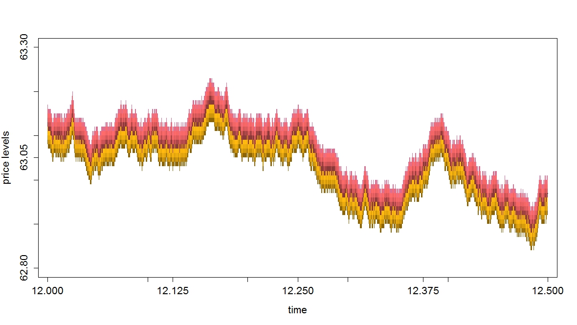
Recently, as information from order books become more and more available, researchers and practitioners have sparked the discussion to which kind of observed prices estimation methods should be applied. [16] discuss this point and the possibilities of mid-quotes, executed traded prices or micro-prices which are volume-weighted combinations of bid and ask order levels. None of these observed time series, however, is free from market microstructure corruptions and the idea of an underlying efficient price remains untouched. Figure 2 visualizes the information about the evolution of prices provided by a limit order book for one specific data set. The colored areas highlight differences between the five best bid and five best ask levels, the dark area in the center marking the bid-ask spread between best bid and best ask. The idea is that an efficient price should lie, at least most of the time, below the best ask (and symmetrically above the best bid) and that its distance to this stochastic frontier is homogeneous. Similar reasoning served as the fundament of the order book model by [27] as well as for the dynamic trading model by [2].

Since modeling in science, economics and particularly finance is always a compromise between catching major features and too complex descriptive models, robustness to model misspecification is a key issue. Therefore we propose a simple modification of our estimator such that occasional violations of the continuous semi-martingale model do not change the asymptotic properties of the estimator. We shall show that for general violations, in particular evoked by jumps of the efficient price and the volatility our adjusted estimation method is robust.

The remainder of the paper is organized as follows. In Section 2 we present an estimation approach based on local order statistics whose asymptotic properties are explored in Section 3, along with the robustification against violations. In Section 4 we prove the lower bound for the minimax estimation rate. An empirical example is performed in Section 5 which concludes with a discussion. Proofs are provided in the Appendix.

We construct the integrated squared volatility estimator in both models (1.2) and (1.3). We partition the unit interval into $h_{n}^{-1}\in\mathds{N}$ equi-spaced bins $\mathcal{T}_{k}^{n}=[kh_{n},(k+1)h_{n}),k=0,\ldots,h_{n}^{-1}-1,$ with bin-widths $h_{n}$. For simplicity suppose that $nh_{n}\in\mathds{N}$. As $n\rightarrow\infty$ the bin-width gets smaller $h_{n}\rightarrow 0$, whereas the number of observed values on each bin gets large, $nh_{n}\rightarrow\infty$. If we think of a constant signal locally on a bin observed with one-sided positive errors, classical parametric estimation theory motivates to use the bin-wise minimum as an estimator of the local signal (it then forms a sufficient statistic under exponential noise or equivalently in the PPP model). In the regression-type model (1.3) with equidistant observation times $t_{i}^{n}=i/n$, we therefore set

Equally, in the PPP model (1.2) the local minima are given by

The same symbol $m_{n,k}$ is used in both models because the following construction only depends on the $m_{n,k}$. All results and proofs will refer to the concrete model under consideration.

Since $\mathbb{V}\hskip-1.42271pt\textnormal{a\hskip 0.56917ptr}(m_{n,k}\,|\,(X_{t}))\propto(n\lambda h_{n})^{-2}$ holds in both models, the variance is much smaller than for an estimator based on a local mean. Nevertheless, we may continue in the spirit of the pre-averaging paradigm, cf. [20], and interpret $m_{n,k}$ as a proxy for $X_{t}$ on ${\cal T}_{k}^{n}$, which in a second step is inserted in the realized variance expression $\sum_{i=1}^{h_{n}^{-1}}(X_{kh_{n}}-X_{(k-1)h_{n}})^{2}$ without noise. The use of a locally constant signal approximation $X_{t}=X_{kh_{n}}+\mathcal{O}_{\mathbb{P}}(h_{n}^{1/2})$ on ${\cal T}_{k}^{n}$ is only admissible, however, if $h_{n}$ is chosen so small that $h_{n}^{1/2}=o((n\lambda h_{n})^{-1})$, which would result in a sub-optimal procedure.

Rate-optimality can be attained if we balance the magnitude $(n\lambda h_{n})^{-1}$ of bin-wise minimal errors due to noise with the range $h_{n}^{1/2}$ of the motion of $X$ on the bin. This gives the order

In the PPP model (1.2) this natural choice of the bin-width also follows nicely by a scaling argument: $\bar{W}_{t}=h_{n}^{-1/2}W_{h_{n}t}$ defines a standard Brownian motion for $t\in[0,1]$ based on the values of $W$ on $[0,h_{n}]$; the correspondingly scaled PPP observations $(\bar{T}_{j},\bar{\cal Y}_{j})$ with $\bar{T}_{j}=h_{n}^{-1}T_{j}$, $\bar{\cal Y}_{j}=h_{n}^{-1/2}{\cal Y}_{j}$ have an intensity with density $\bar{\lambda}_{t,y}=n\lambda h_{n}^{3/2}\mathbbm{1}(y\geq\bar{W}_{t})$, which becomes independent of $n$ exactly for $h_{n}=(n\lambda)^{-2/3}$.

In this balanced setup the law of the statistics $m_{n,k}$ depends on the motion of $X$ as well as the error distribution in a non-trivial way. Still, the natural statistics to assess the quadratic variation of the boundary process $X$ are the squared differences $(m_{n,k}-m_{n,k-1})^{2}$ between consecutive local minima. In the PPP model and with the choice

the law of $h_{n}^{-1/2}m_{n,k}$ is independent of $n$, $h_{n}$ and $\lambda$ and for $X_{t}=X_{(k-1)h_{n}}+\sigma\int_{(k-1)h_{n}}^{t}\,dW_{s}$ on ${\cal T}_{k-1}^{n}\cup{\cal T}_{k}^{n}$, we may introduce

Below we shall derive theoretical properties of $\Psi$ and in particular we shall see that it is invertible as soon as $\mathcal{K}>0$ is chosen sufficiently large. Numerically, the function $\Psi$ can be determined by standard Monte Carlo simulations, see Figure 3, and is thus available. This paves the way for a moment-estimator approach. In fact, $\sum_{k}(m_{n,2k}-m_{n,2k-1})^{2}$ approximates $\int\Psi(\sigma_{t}^{2})dt$ with corresponding summation and integration intervals. Under regularity assumptions on $t\mapsto\sigma_{t}^{2}$ and by the smoothness of $\Psi$ shown below, we have

where $r_{n}^{-1}h_{n}$ is a coarse grid size with $r_{n}h_{n}^{-1}\in\mathds{N},r_{n}^{-1}\in 2\mathds{N}$. This gives rise to the following estimator of integrated squared volatility $IV=\int_{0}^{1}\sigma_{t}^{2}dt$ in the PPP model (1.2) with bin-width (2.4):

In the regression-type model (1.3) the corresponding second moments still depend on $n$ and we write explicitly

We shall see below that $\Psi_{n}\to\Psi$ holds, but a non-asymptotic form of the volatility estimator from regression-type observations is given by

For a parametric estimation of $\sigma_{t}=\sigma=\text{const.}$, we employ the global moment-type estimator $\widehat{IV}_{n}^{h_{n},h_{n}}$. Here, inversion of the entire sum of squared differences is conducted. In the nonparametric case of varying $\sigma_{t}$ instead a localized estimator $\widehat{IV}_{n}^{h_{n},r_{n}}$, with $r_{n}\rightarrow 0,r_{n}^{-1}h_{n}\rightarrow 0$, is applied. A balance between a second order term on each coarse interval of order $r_{n}$ and an approximation error controlled by a semi-martingale assumption on $\sigma_{t}$ of order $r_{n}^{-1}h_{n}$ will lead to the choice $r_{n}\propto h_{n}^{1/2}\propto(n\lambda)^{-1/3}$.

In order to centralize the local minima, we write

where $\mathcal{R}_{n,k}=m_{n,k}-X_{kh_{n}}$ and $\mathcal{L}_{n,k}=m_{n,k-1}-X_{kh_{n}}$ measure the distances between the minima on bin ${\cal T}_{k}^{n}$ and ${\cal T}_{k-1}^{n}$, respectively, to the central true value $X_{kh_{n}}$ between both bins. In our high-frequency framework the drift is asymptotically negligible and a regular volatility function will be approximated by a piecewise constant function on blocks of the coarse grid. In this setting, where $X_{t}=X_{kh_{n}}+\sigma(W_{t}-W_{kh_{n}})$ and $\sigma$ is deterministic, we may invoke time-reversibility of Brownian motion to see that $X_{t}-X_{kh_{n}}$, $t\in{\cal T}_{k-1}^{n}$, and $X_{t}-X_{kh_{n}}$, $t\in{\cal T}_{k}^{n}$, form independent Brownian motions of variance $\sigma^{2}$ such that $\mathcal{R}_{n,k},\mathcal{L}_{n,k},k=(l-1)r_{n}^{-1}+1,\ldots,lr_{n}^{-1}$, are all identically distributed and there is independence whenever different bins are considered (but $\mathcal{R}_{n,k}$ and $\mathcal{L}_{n,k+1}$ are dependent). From (2.5) and (3.1) we infer

and similarly for $\Psi_{n}$. The histogram in Figure 4 shows the distribution of $\mathcal{R}_{n,k}$ (equivalently $\mathcal{L}_{n,k}$) in the regression model jointly with the associated histograms for $\min_{i\in\mathcal{I}_{k}^{n}}X_{t_{i}^{n}}-X_{kh_{n}}$ and $\min_{i\in\mathcal{I}_{k}^{n}}\varepsilon_{i}$. In this situation the law of $\mathcal{R}_{n,k}$ is given as the convolution between an exponential distribution and the law of the minimum of Brownian motion on the discrete grid ${\cal I}_{k}^{n}$. The latter converges to the law of the minimum of $W$ on $[0,1]$, but the simulations confirm the known feature that the laws deviate rather strongly around zero for moderate discretisations. Let us state and prove a slightly more general result.

For the regression-type model the survival function is asymptotically of the same form.

The approximation error due to non-constant $\sigma$ and drift is considered in detail in Appendix A.1 and proved to be asymptotically negligible. This way, the asymptotic analysis of our estimation problem leads into the theory of Brownian excursion areas. Let $\mathcal{R}_{t}$ be a real random variable distributed as $\lim_{n\rightarrow\infty}h_{n}^{-1/2}\mathcal{R}_{n,\lfloor th_{n}^{-1}\rfloor}$. The law of $\mathcal{R}_{t}$ determines $\Psi(\sigma_{t}^{2})$ via

The Feynman–Kac formula gives a connection of the right-hand side in Proposition (3.1) to a parabolic PDE based on the heat semigroup for Brownian motion. We can prove the following explicit result on the Laplace transform which determines the distribution of $(\mathcal{R}_{t}),{t\in[0,1]}$.

This result generalizes the Laplace transform of the exponential integrated positive part of a Brownian motion derived by [31]. Inserting $x=0$ and setting $\vartheta=1$ renders the result by [31]. An inversion of the Laplace transform in Proposition 3.3 in order to obtain an explicit form of the distribution function and then $\Psi$ appears unfeasible as several experts vainly attempted to solve related problems, see [31] and [23]. Exploiting the strong Markov property of Brownian motion together with hitting times, we are able to circumvent this problem in our study of $\Psi(\sigma^{2})$, for details we refer to the Appendix.

The observation models (1.2) and (1.3) as well as the semi-martingale model (1.1) for $X$ might be idealized. In finance, effects of surprise elements and information processing might occasionally result in violations of this model, for instance by price jumps. In such situations, a regularization of $\Psi^{-1}(\cdot)$ can yield more robust estimation results. We propose to truncate the estimator on the coarse grid by employing

for some $\tau>0$ instead of $\Psi^{-1}$, giving the adjusted estimators $\widetilde{IV}_{n,\tau}^{h_{n},r_{n}}$ and $\widehat{IV}_{n,\tau}^{h_{n},r_{n}}$ in (2.7) and (2.9). The truncation level $\tau>0$ is chosen such that we can guarantee $\sup_{t\in[0,1]\setminus\mathcal{V}_{n}}\sigma_{t}^{2}\leq\tau$ almost surely where $\mathcal{V}_{n}$ denotes the union of all violated blocks. In practice, any over-estimated bound from independent historical data may work. Furthermore, observe that any continuous process of finite variation $\bar{A}_{t}$ may corrupt the observations via $Y_{i}=X_{t_{i}^{n}}+A_{t_{i}^{n}}+\varepsilon_{i}$ without harming our volatility estimator because it can be incorporated as a drift into the new semi-martingale $X_{t}+A_{t}$. For order books, the corruption $A_{t_{i}^{n}}$ may account for spreads due to market processing and inventory costs.

We formulate now the main convergence results whose proofs are given in the Appendix. For that we impose some mild regularity on the drift and diffusion coefficient. Moreover, we need that the function $\Psi$ is invertible and sufficiently regular, which by Proposition A.6 below is ensured by a sufficiently large choice of $\mathcal{K}$, but at least numerically seems to be the case for much smaller choices, cf. Figure 3. We work under the general structural hypothesis that the volatility is an Itô semi-martingale with finite activity jumps. This is a standard assumption in financial volatility estimation, see e.g. [4] and [20], allowing for stochastic volatility with leverage. To remain concise, we assume global conditions on the characteristics, but extensions via localization techniques as in Section 4.4.1 of [21] are clearly possible.

Based on the same strategy of proof we can obtain an analogous result for the regression-type model.

In the rate-optimal balanced setup there are three error contributions of the same order: the implied observational noise on the bins $[kh_{n},(k+1)h_{n})$, the bin-wise approximation of $X$, and a second order term on the coarse blocks arising from the nonlinearity of $\Psi$. Their interplay is non-trivial and thus a general stable central limit theorem for the rescaled error does not seem straight-forward. If we dropped the ambition of rate-optimality, however, we could undersmooth or oversmooth by a different choice of the block sizes $h_{n}$ and $r_{n}$ such that only one or two error terms would prevail for which estimators with a simpler asymptotic distribution theory would be available. This is not pursued here.

Consider our PPP-model (1.2). We show that even in the simpler parametric statistical experiment where $X_{t}=\sigma W_{t},\,t\in[0,1]$, and $\sigma>0$ is unknown the optimal rate of convergence is $n^{-1/3}$ in a minimax sense. This lower bound for the parametric case then serves a fortiori as a lower bound for the general nonparametric case. A lower bound for the discrete regression-type model is obtained in a similar way; in fact the proof is even simpler, replacing the Poisson sampling $(T_{j}^{s})$ below by a deterministic design of distance $n^{-2/3}$.

The proof falls into three main parts. We first simplify the problem by considering more informative experiments. These reductions are given in the two steps below. Then, in the third step we use bounds for the Hellinger distance. The more technical step 3 is worked out in Appendix B.

1. 1.

   A PPP with intensity $\Lambda$ is obtained as the sum of two independent PPPs with intensities $\Lambda_{r}$ and $\Lambda_{s}$, respectively, satisfying $\Lambda=\Lambda_{r}+\Lambda_{s}$, see e.g. [25]. Hence, for $b>0$ the experiment of observing $(T_{i}^{r},\mathcal{Y}_{i}^{r})_{i\geq 1}$ from a PPP with regularised intensity density

   $$\lambda_{r}(t,y)=n\Big(\big((y-X_{t})_{+}/b\big)^{2}\wedge 1\Big)$$

   and independently $(T_{j}^{s},\mathcal{Y}_{j}^{s})_{j\geq 1}$ from a PPP with discontinuous intensity density $\lambda_{s}=\lambda-\lambda_{r}$ is more informative. We now provide even more information by replacing $(T_{j}^{s},\mathcal{Y}_{j}^{s})_{j\geq 1}$ by $(T_{j}^{s},X_{T_{j}^{s}})_{j\geq 1}$, the direct observation of the martingale values at the random times $(T_{j}^{s})$. A lower bound proved for observing $(T_{i}^{r},\mathcal{Y}_{i}^{r})_{i\geq 1}$ and $(T_{j}^{s},X_{T_{j}^{s}})_{j\geq 1}$ independently thus also applies to the original (less informative) observations.

2. 2.

   Due to $\int\int\lambda_{s}(t,y)dt\,dy=(2/3)nb$, we conclude that the times $(T_{j}^{s})$ are given by a Poisson sampling of intensity $(2/3)nb$ on $[0,1]$ and there are a.s. only finitely many times $(T_{j}^{s})_{j=1,\ldots,J}$. Let us first work conditionally on $(T_{j}^{s})$ and put $T_{0}^{s}=0$, $T_{J+1}^{s}=1$. All observations of $(T_{i}^{r},\mathcal{Y}_{i}^{r})_{i\geq 1}$ with $T_{i}^{r}\in[T_{j-1}^{s},T_{j}^{s})$ are transformed via

   $$(T_{i}^{r},\mathcal{Y}_{i}^{r})\mapsto\Bigg(T_{i}^{r}-T_{j-1}^{s},\mathcal{Y}_{i}^{r}-\Bigg(X_{T_{j-1}^{s}}\frac{T_{i}^{r}-T_{j-1}^{s}}{T_{j}^{s}-T_{j-1}^{s}}+X_{T_{j}^{s}}\frac{T_{j}^{s}-T_{i}^{r}}{T_{j}^{s}-T_{j-1}^{s}}\Bigg)\Bigg).$$

   Noting that $(B_{t}-(t/T)B_{T},t\in[0,T])$ defines a Brownian bridge $B^{0,T}$ on $[0,T]$, we thus obtain conditionally on $(T_{j}^{s})$ for each $j=1,\ldots,J+1$ observations of a PPP on $\big[0,T_{j}^{s}-T_{j-1}^{s}\big]$ with intensity density

   $$\lambda^{j}(t,y)=n\Big(b^{-1}\big(y-\sigma B^{0,T_{j}^{s}-T_{j-1}^{s}}_{t}\big)_{+}\wedge 1\Big).$$

   The transformation has rendered the family of PPPs with intensity densities $(\lambda^{j})_{j=1,\ldots,J+1}$ independent by reducing the Brownian motion to piecewise Brownian bridges. Conditionally on $(T_{j}^{s})$ we thus have independent observations of $(T_{j}^{s},X_{T_{j}^{s}})_{j=1,\ldots,J}$ and independent PPPs with intensity densities $(\lambda^{j})_{j=1,\ldots,J+1}$.

By using the latter more informative experiment and by choosing $b\propto n^{-1/3}$ we show below that for a Poisson sampling $(T_{j}^{s})_{j=1,\ldots,J}$ on $[0,1]$ of intensity $(2/3)nb\propto n^{2/3}$ of direct observations $X_{T_{j}^{s}}$ as well as for independent observations of PPPs, generated by $\sigma$ times a Brownian bridge in-between the sampling points $(T_{j}^{s})_{j}$, we cannot estimate at a better rate than $n^{-1/3}$. This is accomplished by bounding the Hellinger distance between the experiments for $\sigma^{2}=\sigma_{0}^{2}$ and $\sigma^{2}=\sigma_{0}^{2}+\delta n^{-1/3}$.

For the application to limit order books we model the relationship between ask quotes and an efficient price process by a pure boundary model, not taking into account the fine structure of order book dynamics. This agnostic point of view seems attractive for statistical purposes because more complex models will usually require more data for the same estimation accuracy and are highly exposed to model misspecification. To check whether the semi-martingale boundary model leads to realistic results, we apply our estimator to limit order book data and compare it to integrated volatility estimators, which are commonly used for traded prices under market microstructure noise.

We consider limit order book data of the Facebook asset (FB) traded at NASDAQ provided by LOBSTER academic data, recorded over the 21 trading days in August 2015. Empirical data analysis with similar assets lead to comparable results. The August 2015 time series has the advantage of starting with a relatively calm period before incorporating a period of high trading activity, which can serve as a kind of stress test to the estimators. We estimate day-wise integrated volatilities based on

1. 1.

   Our estimator (2.9) with truncation for the regression-type model and first level ask quotes log-prices (and symmetrically, but independently bid quotes), called $\widehat{IV}$ in the sequel. The average number of newly submitted best ask quotes per day, $n$, in the considered period is about 100,000. The average $n$ for bid quotes is similar, but the difference on certain days may be large. The maximal absolute difference is 30,537 in the considered period.

2. 2.

   The local method of moment (LMM) estimator from [6], adjusted to possible jumps with the truncated version from [8], and log-prices from trades reconstructed from the order book. The average number of trades per day in the considered period is about 43,000.

The LMM is the asymptotically efficient estimator for the standard regular noise model with centered noise and we follow the implementation with a selection of tuning parameter described in [7]. For the truncation step we employ a global threshold $\tau=2\log(h_{n}^{-1})h_{n}\widehat{IV}^{pre}$, with the pre-estimator of integrated volatility obtained from the first estimation step of the two-stage adaptive LMM, for both approaches using their different bin-lengths $h_{n}$ and sample sizes $n$. $h_{n}$ is chosen in a data-driven way, for the LMM we arrive at about 100 bins per day and for the $\widehat{IV}$ at about 650 bins. We expect that comparative studies using alternative estimators for the regular noise model, as e.g. realized kernels from [4] or pre-averaging from [20], would yield similar results.

The results are presented in Figure 5. It shows a rather close relationship between the three sequences of estimates. Estimates obtained from bid and ask quotes can differ, but their differences are very small. On August 24, 2015, however, there is a large difference among the estimators. On that day a flash crash manipulated the traded and order quote prices challenging all market models. The huge difference among the truncated estimates is due to the rougher time resolution of bins for LMM which are equidistant in calendar time. The flash crash led to tremendous price movements in very short time at the beginning of the trading day along with a huge trading activity. In the regular noise model the LMM ascribes those movements on its first two time bins to jumps and truncates, while our bin widths $h_{n}$ are much smaller and thus $\widehat{IV}$ is still affected by this period because not all bins are truncated. The same effect explains why the values of $\widehat{IV}$ are significantly larger around that date.

A priori, even from a microeconomic perspective, it is not clear whether the assumed efficient price processes for the different market mechanisms giving rise to bids, asks and trades are the same or at least exhibit the same integrated volatility. A proper statistical test for the latter hypothesis requires a simultaneous distribution theory for $\widehat{IV}$ and the LMM (a CLT alone is not sufficient), which is beyond the scope of the present work and a project in its own right. For the LMM alone, however, a feasible central limit theorem is available, see Theorem 4.4 of [6].

For the Facebook data set we have conducted a test on the hypothesis that the integrated volatilities in the order book and transaction price models coincide, assuming independence of the estimators and a Gaussian limit distribution where the variance of $\widehat{IV}$ does not exceed the one of LMM. Applied to 21 trading days and at asymptotic level $\alpha=5\%$ , the test has accepted the null on 14 days and rejected on 7 days. This testing problem illustrates that more mathematical analysis of the estimator’s risk is highly desirable as well as a more profound empirical study.

Proposition 3.2 considers the simplified model where $X_{t},t\in{\cal T}_{k}^{n}$, is approximated by $X_{kh_{n}}+\int_{kh_{n}}^{t}\sigma_{kh_{n}}\,dW_{t}$. The resulting approximation error is bounded within Proposition A.2 for the PPP-model and an analogous proof carries over to the regression-type model. In the sequel, we write $A_{+}=A\mathbbm{1}(A\geq 0)$, $A_{-}=|A|\mathbbm{1}{(A\leq 0)}$ and $\|Z\|_{p}=\mathbb{E}[|Z|^{p}]^{1/p},p\geq 1$.

References

- [1] Aït-Sahalia, Y., Mykland, P. A. and Zhang, L. (2005). How often to sample a continuous-time process in the presence of market microstructure noise. Review of Financial Studies, 18, 351–416.
- [2] Aït-Sahalia, Y. and Saglam, M. (2014). High Frequency Traders: Taking Advantage of Speed. preprint, SSRN: 2331613.
- [3] Bacry, E. and Muzy, J. F. (2014). Hawkes model for price and trades high-frequency dynamics. Quantitative Finance, 14 (7), 1147–1166.
- [4] Barndorff-Nielsen, O. E., Hansen, P. R., Lunde, A. and Shephard, N. (2008). Designing realised kernels to measure the ex-post variation of equity prices in the presence of noise. Econometrica 76 (6), 1481–1536.
- [5] Biais, B., Hillion, P. and Spatt, C. (1995). An empirical analysis of the limit order book and the order flow in the paris bourse. The Journal of Finance, 50 (5), 1655–1689.
- [6] Bibinger, M., Hautsch, N., Malec, P. and Reiß, M. (2014). Estimating the Quadratic Covariation Matrix from Noisy Observations: Local Method of Moments and Efficiency, The Annals of Statistics, 42 (4), 1312–1346.
- [7] Bibinger, M., Hautsch, N., Malec, P. and Reiß, M. (2014). Estimating the Spot Covariation of Asset Prices – Statistical Theory and Empirical Evidence, CFS Working Paper, No. 477, SSRN:2507714.
- [8] Bibinger, M. and Winkelmann, L. (2015). Econometrics of co-jumps in high-frequency data with noise. The Journal of Econometrics, 184, 361–378.
- [9] Bouchaud, J. P., Mzard, M. and Potters, M. (2002). Statistical properties of stock order books: Empirical results and models. Quantitative Finance, 2 (4), 251–256.
- [10] Carmona, R. and Lacker, D. (2015). A probabilistic weak formulation of mean field games and applications. The Annals of Applied Probability, 25 (3), 1189–1231.
- [11] Clément, E., Delattre, S. and Gloter, A. (2013). An infinite dimensional convolution theorem with applications to the efficient estimation of the integrated volatility. Stochastic Processes and their Applications, 123 (7), 2500–2521.
- [12] Cont, R., Stoikov, S. and Talreja, R. (2010). A stochastic model for order book dynamics. Operations Research, 58 (3), 549–563.
- [13] Cont, R. and de Larrard, A. (2012). Order Book Dynamics in Liquid Markets: Limit Theorems and Diffusion Approximations. preprint, SSRN: http://ssrn.com/abstract=1757861
- [14] Diaz, H. F. and Hughes, M. K. and Swetman, T. W. (2010). Dendroclimatology: progress and prospects. Springer Netherlands.
- [15] Foucault, T., Kadan, O. and Kandel, E. (2005). Limit order book as a market for liquidity. Review of Financial Studies, 18, 1171–1217.
- [16] Gatheral, J. and Oomen, R. C. A. (2010). Zero-Intelligence Realized Variance Estimation. Finance and Stochastics, 14 (2), 249–283.
- [17] Glosten, L.R. and Milgrom, P. R. (1985). Bid, ask and transaction prices in a specialist market with heterogeneously informed traders. Journal of Financial Economics, 14, 71–100.
- [18] Gloter, A. and Jacod, J. (2001). Diffusions with measurement errors 1 and 2. ESAIM, Probability and Statistics, 5, 225–242.
- [19] Imkeller, P. and Storch, J-S. (2012). Stochastic Climate Models. In Progress in Probability, Basel: Birkhäuser.
- [20] Jacod, J., Podolskij, M. and Vetter, M. (2010). Limit theorems for moving averages of discretized processes plus noise. The Annals of Statistics 38 (3), 1478–1545.
- [21] Jacod, J. and Protter, P. (2012). Discretization of processes. New York: Springer.
- [22] Jaisson, T. and Rosenbaum, M. (2014). Limit theorems for nearly unstable Hawkes processes. The Annals of Applied Probability, 25 (2), 600–631.
- [23] Janson, S. (2007). Brownian excursion area, Wright’s constants in graph enumeration, and other Brownian areas. Probability Surveys 4, 80–145.
- [24] Karatzas, I. and Shreve, S. E. (1991). Brownian motion and stochastic calculus. Second Edition. Volume 113 of Graduate Texts in Mathematics. New York: Springer-Verlag.
- [25] Karr, A. F. (1991). Point processes and their statistical inference. Second edition. Probability: Pure and Applied, New York: Marcel Dekker, Inc.
- [26] Kutoyants, Y. (1998). Statistical Inference for Spatial Poisson Processes. Lecture Notes in Statistics, Springer.
- [27] Lorenz, J. and Osterrieder, J. (2009). Simulation of a limit order driven market. The Journal of Trading, 4 (1), 23–30.
- [28] Majda, A. J. and Timofeyev, I. and Eijnden, E. V. (2001). A mathematical framework for stochastic climate models. Comm. Pure Appl. Math., 54 (8), 891–974.
- [29] Meister, A. and Reiß, M. (2013). Asymptotic equivalence for nonparametric regression with non-regular errors. Probability Theory and Related Fields 155, (1-2), 201–229. Proceedings of the 7th Séminaire Européen de
- [30] Naes, R. and Skjeltorp, J. A. (2006). Order book characteristics and the volume-volatility relation: Empirical evidence from a limit order market. Journal of Financial Markets, 9 (4), 408–432.
- [31] Perman, M. and Wellner, J. A. (1996). On the distribution of Brownian areas. The Annals of Applied Probability 6 (4), 1091–1111.
- [32] Reiß, M. (2011). Asymptotic equivalence for inference on the volatility from noisy observations. The Annals of Statistics, 39 (2), 772–802.
- [33] Rosu, I. (2009). A dynamic model of the limit order book. Review of Financial Studies, 22 (11), 4601–4641.
- [34] Tsybakov, A. B. (2009). Introduction to Nonparametric Estimation. New York: Springer-Verlag.
- [35] Varlamov, V. (2008). Differential and integral relations involving fractional derivatives of Airy functions and applications. Journal of Mathematical Analysis and Applications 348 (1), 101–115.
- [36] Zhang, L., Mykland, P. A. and Aït-Sahalia, Y. (2005). A tale of two time scales: Determining integrated volatility with noisy high-frequency data. Journal of the American Statistical Association 100 (472), 1394–1411.