跳到论文正文
W Papers独立论文阅读器 arXiv:1408.3661 论文正文 计算阅读时间 · 0%
引用这篇论文根据当前论文元数据生成,正式投稿前建议核对。


License: arXiv.org perpetual non-exclusive license
arXiv:1408.3661v1 [cs.IT] 15 Aug 2014

Overhead Performance Tradeoffs—A Resource Allocation Perspective

Jie Ren    Bradford D. Boyle    Gwanmo Ku    Steven Weber    John MacLaren Walsh ††thanks: This research has been supported by the Air Force Research Laboratory under agreement number FA9550-12-1-0086. The U.S. Government is authorized to reproduce and distribute reprints for Governmental purposes notwithstanding any copyright notation thereon.††thanks: The authors are with the Department of Electrical and Computer Engineering, Drexel University, Philadelphia, PA USA. The contact author is John MacLaren Walsh (email: jwalsh@ece.drexel.edu)††thanks: Preliminary results were reported at CISS 2014 [1, 2].
Abstract

A key aspect of many resource allocation problems is the need for the resource controller to compute a function, such as the max\max or arg​max\argmax, of the competing users metrics. Information must be exchanged between the competing users and the resource controller in order for this function to be computed. In many practical resource controllers the competing users’ metrics are communicated to the resource controller, which then computes the desired extremization function. However, in this paper it is shown that information rate savings can be obtained by recognizing that controller only needs to determine the result of this extremization function. If the extremization function is to be computed losslessly, the rate savings are shown in most cases to be at most 22 bits independent of the number of competing users. Motivated by the small savings in the lossless case, simple achievable schemes for both the lossy and interactive variants of this problem are considered. It is shown that both of these approaches have the potential to realize large rate savings, especially in the case where the number of competing users is large. For the lossy variant, it is shown that the proposed simple achievable schemes are in fact close to the fundamental limit given by the rate distortion function.

Index Terms: 
Distributed function computation, extremization, rate distortion, scalar quantization, interactive communication, resource allocation

I Introduction

In this paper we consider a problem in which series of NN users have access to independent sequences 𝑿i=[Xi,s|s∈{1,2,…,}],i∈{1,…,N}\bm{X}_{i}=\left[X_{i,s}|s\in\{1,2,\ldots,\}\right],\ i\in\{1,\ldots,N\} of independent and identically distributed observations Xi,sX_{i,s} from a known distribution on a set 𝒳⊂ℝ+\mathcal{X}\subset\mathbb{R}^{+}, a subset of the non-negative real numbers. The users compress their observations for transmission to a CEO (CEO) that wishes to know for each element in the sequence:

  1. 1.

    the largest observation, i.e. maxi∈{1,…,N}⁡Xi,s\max_{i\in\{1,\ldots,N\}}X_{i,s} for each ss;

  2. 2.

    a source having the largest observation, i.e. a single member of arg⁡maxi∈{1,…,N}⁡Xi,s\arg\max_{i\in\{1,\ldots,N\}}X_{i,s} for each ss, or;

  3. 3.

    both the largest observation and the user that having the largest observation.

We refer the three cases as the max\max problem, the arg​max\argmax problem, and the (max,arg​max)(\max,\argmax) problem respectively. Although we present all our results terms of max\max, similar results will hold for the corresponding minimization problems.

(a)
(b)
Fig. 1: Model block diagrams
max\max arg​max\argmax (max,arg​max)(\max,\argmax)
1 OFDMA resource allocation anycasting rateless PHY layer traditional AMC PHY layer
2 economics asset pricing asset allocation sealed-bid first-price auctions
3 sensor network/intrusion detection is there an intruder where is the intruder is there an intruder & where is the intruder
TABLE I: Example application of indirect extremal value computation

This generic indirect extremal value computation problem finds examples in several fields; Table I lists a few of these. We consider three in more detail here:

Example 1 ( OFDMA (OFDMA) resource allocation).

Rateless coding, also known as fixed-to-variable coding [3], can achieve performance close to the channel capacity without requiring the explicit feedback of channel state information and use of adaptive modulation and coding in a single user system [4, 5]. These schemes operate by enabling the block length (in channel uses) for the modulation and coding to stretch or shrink based on the received channel quality in a manner that closely resembles H-ARQ. Rather than feeding back channel quality, the receiver only needs to indicate when it has successfully decoded the transmitted message, which it learns through an outer error detection code. In a multiuser OFDMA system, the BS (BS) needs to assign MS to subblocks of channles, even when a rateless code used (Fig. 2). If the BS wishes to maximize the sum-rate across users, the uplink feedback from the MS only needs to enable the basestation to determine which MS has the best channel. The BS does not need to know the actual channel gain/capacity.

Refer to caption
Fig. 2: The BS wishes to compute the index (arg max) of the user with the largest gain on each subband. The users encode their local gains across subbands using SQ.

Once the BS has decided which user to schedule on a particular collection of subbands, it must signal this resource decision on the downlink as overhead control information in addition to the data to be transmitted to the user itself. These resource decisions control information, along with the MS’s feedback, result in control overheads that are surprisingly large—the control overheads account for ≈25\approx 25–30%30\% of all downlink transmission in the LTE standard[6].

Anycasting is transmission scheme whereby a sender wishes to send a message to a group of potential receivers and ensure that it is received by at least one receiver [7]. This is contrasted with broadcasting, where every receiver is required to receive the message. In this context, the CEO is the BS and the sourcess at the different receivers are the channel gains/capacities on the downlinks. The BS needs to know the largest channel capacity in order to select an approriate transmission rate. Replacing max\max with min\min, this setup becomes a broadcasting problem. By knowing the smallest channel capacity, the BS can select a rate that ensures its message is received by all of the users.

Traditional AMC (AMC) [8] proceeds by first defining a finite collection of codes and modulation schemes associated with different information rates rkr_{k} measured in bits per channel use. The index k∈{1,…,K}k\in\{1,\ldots,K\} indicating which scheme to use is called the MCS (MCS) index. The receiver measures the channel quality using reference or training signals, or pilots, and determines the information rate among this finite set corresponding to a modulation and coding scheme achieving a given target probability of error. The associated index kk, or some quantization of it, is then fed back to the transmitter under the label CQI (CQI). The transmitter then takes into consideration factors such as the amount of data waiting to be sent to the various receivers associated with it and their necessary quality of service, then selects the modulation and coding scheme to use when transmitting to them.

Example 2 (Economics).

When a seller has a commodity that it wishes to sell, it sets the price with respect to the market [9]. If the seller wants to ensure that it does not price it self out of the market, it would want to compute the max\max of the individual valuations of a representative sample of the market. Conversely, if the seller wants to undercut its competition it would need to compute the min\min of the competitor’s prices.

In many situations, goods should be allocated/distributed to users based on their “need” or expected derived utility [10]. For example, need-based financial aid for higher education. In this scenario, the entity distributing the goods would only need to calculate the individual with the largest expected derived utility (i.e., the arg​max\argmax).

We think of the CEO selling a good through an auction to a set of independent buyers. In a sealed-bid first-price auction, the buyers submit bids in “sealed” envelopes and the highest bidder is the winner, paying their bid amount[11]. The auctioneer has no need for recovering this bids of the other users.

Example 3 (Sensor network/intrusion detection [12]).

A collection of sensor nodes are monitoring an area large enough that individual sensor readings are independent. As a very simple model, we can take the local sensor outputs to be binary: 00 if no intruder is present, 11 if an intruder is present. Computing the arg​max\argmax determines where an intruder is (if in fact there is one); computing themax\max sensor reading determines if an intruder is present but not where, and; computing both determines if and where an intruder is.

The remainder of the paper is organized as follows: In Section II, we review the existing literature concerning fundamental limits and achievable schemes for the non-interactive lossless and lossy estimation. We also review literature for the interactive variant of this problem where the users and CEO are allowed to interactively communicate over multiple rounds. Next we formalize the mathematical model for this problem and propose natural distortion measures in Section III. In Section IV, we derive the fundamental limit on rate to estimate losslessly (in the usual Shannon sense) and propose a scheme to achieve this limit. We observe that the rate savings compared with the source recovery (i.e. SW (SW) [13]) are not large. In Section V, we consider the same problem, but allow the CEO to estimate the function in a lossy manner. We compute the rate-distortion function numerically (Section V-A) and compare it with an achievable scheme based on scalar quantization (Section V-B & Section V-C). Finally in Section VI, we consider interactive communications[14] between the CEO and the users. We propose interactive schemes in which the CEO will losslessly determine the max\max, arg​max\argmax or the pair. For both the one-shot lossy and interactive lossless case, we show the rate saving can be substantial.

II Related Work

We first review some previous results of the CEO problem under both lossless and lossy setup to understand the fundamental limits of the rate region. We then review some results about quantization design which help us to give achievable schemes for the extremization problems we are interested in.We will also cover the lossless interactive communication results which allows multi-round communications. In this paper, we consider aymptotically lossless, lossy (i.e., rate-distortion), and interactive limits for the problem of computing the functions of interest. In this section we review the literature for the different approaches to the problem as well as the literature on quantization-based achievable schemes.

II-A Related Work—Lossless

The two-terminal function computation with side information problem has been considered in [15] and [16] where two terminals (transmitter and receiver) each contain a source and the receiver wants to decode a function of the two sources. Earlier work by Witsenhausen considered the problem of minimizing the encoder’s alphabet size with the constraint that the computation needs to be zero-error[15]. He showed the minimum alphabet size is related to the chromatic number of the characteristic graph of the source. Orlitsky et al. considered a similar problem setup, but instead of zero-error they allowed an asymptotically small probability of error[16]. With this assumption, they showed the fundamental limit on rate is the graph entropy of the characteristic graph. The distributed function computation problem has been considered in [17] and [18] where the problem is under the CEO setup[19] where the CEO wants to compute a function of the sources from two or more users. Doshi et al. gave the rate region to the problem under a constraint that they term a “zig-zag” condition [18]. They showed that any achievable rate point can be realized by graph coloring at each user and SW encoding the colors. Sefidgaran et al. derived inner and outer bounds to the rate region under for a class of tree structured networks, which includes the classical CEO problem formulation. They also showed that the two bounds coincide with each other if the sources are independent and hence obtained an expression for the rate region [17]. The extremization functions that we are interested in are set-valued and the CEO only needs to know one value rather than the whole set of the function result. Under this setup, we give the fundamental limits of the minimum sum-rate to losslessly determine the extremizations. These results are in agreement with the results in [17] and [18] when the function is single-valued.

II-B Related Work—Lossy

After Shannon introduced rate distortion function in source coding with a fidelity criterion [20], rate distortion theory was notably developed by Berger and Gallager [21, 22]. Recent work in rate distortion theory has been focused on lossy source coding by attempting to find efficient compression algorithms based on information theory. Rate distortion theory was extended to multi-terminal systems in the 1970’s by Berger and Tung [23, 24]. For point-to-point rate distortion problems, Arimoto and Blahut proposed numerical calculation algorithms based on alternating optimization to find the channel capacity and rate distortion function [25, 26]. The convergence proof of Blahut and Arimoto’ algorithms was developed by Csiszar [27] and Boukris [28]. The generic CEO problem from multi-terminal source coding theory was introduced by Berger [19] and the Quadratic Gaussian CEO rate region is known by Oohama [29] and Prabhakaran [30]. A general outer bound to the CEO problem, not necessarily required Quadratic Gaussian CEO problem, was derived by Wagner [31]. Lossy indirect function computation at the CEO was developed by Oohama [29] and Wyner [32]. An adaptation of the Blahut-Arimoto algorithm to the CEO model with independent sources is developed by the authors [33].

II-C Related Work—Scaler Quantization

Recent work by Misra et al. considered the problem of DFSQ (DFSQ) [34]. By focusing on the high-rate regime and assuming a MSE (MSE) distortion, the authors are able to make several approximations to obtain distortion expressions that are optimal asymptotically (i.e., as the rate goes to infinity). We assume a different distortion measure, derive an exact expression for the distortion as a function of the quantizer parameters, and derive necessary conditions for optimal parameters. Moreover, our results hold for all rates.

Our focus on the use of SQ as an achievable scheme is motivated by several results concerning the optimality of a layered architecture of quantization followed by entropy coding. Zamir et al. considered the distributed encoding and centralized decoding of continuous valued sources and established that lattice quantization followed by SW encoding is optimal asymptotically in rate [35]. When the sources are Gaussian and the distortion is MSE, local vector quantizers followed by SW coding is optimal, not just asymptotically [36]. For discrete valued random variables, scalar quantization with block entropy encoding is optimal [37]. Each of the problem models considered in [35, 36, 37] can be understood as an instance of indirect distributed lossy source coding for the identity function.

II-D Related Work—Interaction

Interactive communication is the scheme that allows message passing forward and backward multiple times between two or more terminals. For the two terminals’ interactive communication problem of lossy source reproduction, Kaspi first characterized the rate region in [38]. Followed by this, Ishwar and Ma made some further contributions. They worked on both two and more than two terminals cases for computing any function of the sources in both lossy and lossless manner. They showed that interactive communication strictly improves the Wyner-Ziv rate-distortion function[39]. They also showed that in some distributed function computation problems, interactive communication can provide substantial benefits over non-interactive codes and infinite-many rounds of interaction may still improve the rate-region[14]. In Section VI, we consider resource allocation in the multiuser OFDMA systems that use rateless AWGN codes for downlink data transmission as a model of the distributed arg-max problem. We propose an interactive communication scheme for this resource allocation problem. This scheme is inspired by the ideas of selective multiuser diversity [40] (SMUD) scheme as well as the multi-predefined thresholds [41] scheme which is an extension of SMUD that set up multiple thresholds and allow the user nodes sending messages based on these thresholds.

III Model Specification

As stated previously, we are considering the NN user CEO problem for estimating either max\max, arg​max\argmax, or the pair (max,arg​max)(\max,\argmax). The i​thi\textsuperscript{th} user observes the sequence 𝑿i≜(Xi,s:s∈[S])\bm{X}_{i}\triangleq(X_{i,s}:s\in[S]) of non-negative random variables 11 1 For any integer nn, let [n]≜{1,…,n}[n]\triangleq\{1,\ldots,n\}. Let 𝑿≜(𝑿i:i∈[N])\bm{X}\triangleq(\bm{X}_{i}:i\in[N]). We assume that the sources are independent and identically distributed (i.i.d.) across both users (ii) and the sequence (ss); that is

f𝑿​(𝒙)=∏i=1N∏s=1SfX​(xn,s).f_{\bm{X}}(\bm{x})=\prod_{i=1}^{N}\prod_{s=1}^{S}f_{X}(x_{n,s}). (1)

The quantities we are interested in for our problem are

ZA​(s)≜{i|Xi,s=max⁡{Xi,s:i∈[N]}}Z_{A}(s)\triangleq\{i|X_{i,s}=\max\{X_{i,s}:i\in[N]\}\} (2)

as the users with the maximum s​ths\textsuperscript{th} source output and

ZM​(s)≜max⁡{Xi,s:i∈[N]}Z_{M}(s)\triangleq\max\{X_{i,s}:i\in[N]\} (3)

as the maximum s​ths\textsuperscript{th} source output. Specifically for the arg​max\argmax case, we consider a class of problems where we need not estimate the set ZA​(s)Z_{A}(s), but rather a representative user from this set.

TABLE II: Notation Guide
Symbol Meaning
𝒞⁡(G⁡(f))\mathcal{C}(G(f)) set of all coloring method to color GG
c⁡(xi)c(x_{i}) coloring of source xix_{i}
ℓ\bm{\ell} scalar quantizer decision boundaries
ϵ\epsilon fixed, but arbitrarily small value
EkE_{k} 𝔼⁡[X|ℓk−1≤X≤ℓk]\mathds{E}\left[X|\ell_{k-1}\leq X\leq\ell_{k}\right]
ff probability density function
fkf_{k} fX​(ℓk)f_{X}(\ell_{k})
FF cumulative density function
FkF_{k} FX​(ℓk)F_{X}(\ell_{k})
gg generic optimal resource allocation function
G⁡(V,E)G(V,E) non directed graph with vertex set V and edge set E
hh binary entropy function −p​log2​p−(1−p)​log2⁡(1−p)-p\log_{2}p-(1-p)\log_{2}(1-p)
H⁡(⋅)H(\cdot) Shannon entropy
HGH_{G} graph entropy
ii user indexing variable
jj subcarrier indexing variable
i,ji,j possible CQI levels/nodes in G usually in the proof in lossless limit section
kk quantizer level indexing variable
KK number of quantizer bins
κ\kappa rate region in Doshi’s result
L⁡(ℓ,𝝁)L(\bm{\ell},\bm{\mu}) Lagrangian
Lf​(X1|X2)L_{f}(X_{1}|X_{2}) fundamental limit of the one-way Orlitsky’s problem
ℒk\mathcal{L}_{k} kkth quantizer bin
MiM_{i} message index for iith user
NN number of users
nn user indexing variable
pp shorthand for probability
pkp_{k} FX​(ℓk)−FX​(ℓk−1)F_{X}(\ell_{k})-F_{X}(\ell_{k-1})
RR total rate from all users
RiR_{i} rate from user ii
RH​o​m​S​QR_{HomSQ} rate of HomSQ (HomSQ)
RH​e​t​S​QR_{HetSQ} rate of HetSQ (HetSQ)
ss sequence indexing variable
SS size of the source sequence
tt discrete time index
UtU_{t} message sent from the BS to MSs at round t in interaction scheme
Γ⁡(G)\Gamma(G) set of maximum independent sets of a graph
WW maximum independent set
XX random variable for channel capacity
𝒳\mathcal{X} support set for random variable XX
ZZ generic resource allocation
ZAZ_{A} arg-max of values
ZMZ_{M} max of values
ZM,AZ_{M,A} both max & arg-max of values
λ\lambda possible threshold in interaction scheme
λt∗\lambda^{*}_{t} optimal threshold at round t in interaction scheme
μ\mu Lagrange multiplier (slope) for rate-distortion computation
ν\nu Lagrange multiplier associated with equality constraints
ϕ\phi encoding mapping
ψ\psi decoding mapping

III-A Distortion Measures

Two typical distortion measures are Hamming and squared error, neither of which are appropriate for the problems of interest (Section I, Examples 1–3). Hamming distortion is “all-or-nothing” in that all estimation errors are treated the same. Squared error distortion more heavily penalizes larger estimation errors, but treats under- and over-estimation the same. For the problems of interest, over-estimation needs to be more heavily penalized then under-estimation. With that in mind, we propose the following distortion measures. For estimating the max\max, the distortion measures linearly penalizes underestimation of the maximum value; we can think of this as the lost revenue (difference between what you could have gotten and what you got) when an asset is priced below market value. It also captures the loss when the estimated max rate exceeds the actual max; continuing the analogy, this is the case where an asset does not sell because it is priced above market value.

dM​((X1,s,…,XN,s),Z^M​(s))={ZM​(s)−Z^M​(s)if Z^M​(s)≤ZM​(s)ZM​(s)otherwised_{M}((X_{1,s},\ldots,X_{N,s}),\hat{Z}_{M}(s))=\begin{cases}Z_{M}(s)-\hat{Z}_{M}(s)&if $\hat{Z}_{M}(s)\leq Z_{M}(s)$\\ Z_{M}(s)&otherwise\end{cases} (4)

For estimating the arg​max\argmax, a similar distortion measure is utilized. The distortion measures the loss between source value of the user with the actual max and the source value for the user estimated to have the max. Unlike the previous case, the CEO cannot make an over-estimation error.

dA​((X1,s,…,XN,s),Z^A​(s))={0if Z^A∈ZAZM​(s)−XZ^A​(s),sotherwised_{A}((X_{1,s},\ldots,X_{N,s}),\hat{Z}_{A}(s))=\begin{cases}0&if $\hat{Z}_{A}\in Z_{A}$\\ Z_{M}(s)-X_{\hat{Z}_{A}(s),s}&otherwise\end{cases} (5)

Finally, for estimating the pair of values (max,arg​max)(\max,\argmax) we propose a distortion measure that is a hybrid of the previous two. The distortion is a combination of under-estimating the max value, provided the estimate does not exceed the value of the user estimated as having the max value. It also captures the loss due to over-estimation, both exceeding the estimated arg​max\argmax user’s value or exceeding the actual max value.

dM,A​((X1,s,…,XN,s),(Z^M​(s),Z^A​(s)))={ZM−Z^M​(s)if Z^M​(s)≤XZ^A​(s),sZMotherwised_{M,A}((X_{1,s},\ldots,X_{N,s}),(\hat{Z}_{M}(s),\hat{Z}_{A}(s)))=\begin{cases}Z_{M}-\hat{Z}_{M}(s)&if $\hat{Z}_{M}(s)\leq X_{\hat{Z}_{A}(s),s}$\\ Z_{M}&otherwise\end{cases} (6)

Depending on the problem formulation being considered, let d⁡(s)d(s) be

  1. 1.

    dM,A​((X1,s,…,XN,s),(Z^M​(s),Z^A​(s)))d_{M,A}((X_{1,s},\ldots,X_{N,s}),(\hat{Z}_{M}(s),\hat{Z}_{A}(s)));

  2. 2.

    dA​((X1,s,…,XN,s),Z^A​(s))d_{A}((X_{1,s},\ldots,X_{N,s}),\hat{Z}_{A}(s)), or;

  3. 3.

    dM​((X1,s,…,XN,s),Z^M​(s))d_{M}((X_{1,s},\ldots,X_{N,s}),\hat{Z}_{M}(s))

and define

d⁡((𝑿1,…,𝑿N),𝒁^)=1S​∑s=1Sd⁡(s)d((\bm{X}_{1},\ldots,\bm{X}_{N}),\hat{\bm{Z}})=\frac{1}{S}\sum_{s=1}^{S}d(s) (7)

as the distortion between sequences. Finally, denote

D=𝔼⁡[d⁡((𝑿1,…,𝑿N),𝒁^)]D=\mathds{E}\left[d((\bm{X}_{1},\ldots,\bm{X}_{N}),\hat{\bm{Z}})\right] (8)

where the expectation is with respect to joint distribution on the sources. In the next section, we consider the problem of finding the minimum sum rate necessary for computing the different extremization functions when the distortion is constrained D=0D=0. Later, we will consider the problem of the minimum sum rate necessary for computing the different extremization functions with a non-zero upper bound on the distortion DD.

IV Lossless Extremization

In this section, we determine the minimum amount of information necessary to remotely solve the extremization problems in a Shannon lossless sense. We begin by providing an achievable scheme for the arg​max\argmax problem based on graph coloring in Section IV-A. We then prove in Section IV-B that this scheme achieves a fundamental limit. We also show via a computation of the fundamental limits, that no rate can be saved relative to simply forwarding the observations in the max\max and (max,arg​max)(\max,\argmax) problems unless min⁡𝒳=0\min\mathcal{X}=0.

In [16], a related problem is considered in which the node observing 𝑿1\bm{X}_{1} sends a message to the node observing 𝑿2\bm{X}_{2} in such a manner that the function 𝒇S​(𝑿1S,𝑿2S)=[f⁡(X1,s,X2,s)|s∈[S]]\bm{f}^{S}(\bm{X}_{1}^{S},\bm{X}_{2}^{S})=[f(X_{1,s},X_{2,s})|s\in[S]], taking values from the set 𝒵S\mathcal{Z}^{S}, can be computed losslessly. In this problem, a rate RR is said to be achievable if for every ϵ>0\epsilon>0 there exists a sufficiently large SS and KK with R≥KSR\geq\frac{K}{S}, and an encoder φ:𝒳S→{0,1}K\varphi:\mathcal{X}^{S}\rightarrow\{0,1\}^{K} and a decoder ψ:{0,1}K×𝒳S→𝒵S\psi:\{0,1\}^{K}\times\mathcal{X}^{S}\rightarrow\mathcal{Z}^{S} such that ℙ⁡(ψ⁡(φ⁡(𝑿1S),𝑿2S)≠𝒇S​(𝑿1S,𝑿2S))<ϵ\mathbb{P}(\psi(\varphi(\bm{X}_{1}^{S}),\bm{X}_{2}^{S})\neq\bm{f}^{S}(\bm{X}_{1}^{S},\bm{X}_{2}^{S}))<\epsilon. Orlitsky and Roche proved that for given X1X_{1}, X2X_{2} and ff, the infimum of the set of achievable rates is

Lf​(X1|X2)=HG​(X1|X2)L_{f}(X_{1}|X_{2})=H_{G}(X_{1}|X_{2}) (9)

where HG​(X1|X2)H_{G}(X_{1}|X_{2}) is the conditional graph entropy of the characteristic graph of this problem in [16]. The characteristic graph GG of X1X_{1}, X2X_{2}, and ff is a generalization of the definition given by Witsenhausen[15]. Its vertex set is the support set 𝒳\mathcal{X} of X1X_{1}, and distinct vertices x1x_{1}, x1′x_{1}^{\prime} are adjacent if there is a x2x_{2} such that p⁡(x1,x2),p⁡(x1′,x2)>0p(x_{1},x_{2}),p(x_{1}^{\prime},x_{2})>0 and f⁡(x1,x2)≠f⁡(x1′,x2)f(x_{1},x_{2})\neq f(x_{1}^{\prime},x_{2}). The conditional graph entropy is

HG​(X1|X2)≜minW−X1−X2,X1∈W∈Γ⁡(G)⁡I⁡(W;X1|X2)H_{G}(X_{1}|X_{2})\triangleq\min_{W-X_{1}-X_{2},X_{1}\in W\in\Gamma(G)}I(W;X_{1}|X_{2}) (10)

where Γ⁡(G)\Gamma(G) is the set of all maximal independent sets in GG, WW is a random variable that has Γ⁡(G)\Gamma(G) as its support set, and the minimization is over all conditional probabilities p⁡(w|x1)p(w|x_{1}) which is supported on those maximal independent sets ww containing the vertex x1x_{1}, with the constraint that WW, X1X_{1} and X2X_{2} form a Markov chain.

Additionally, conditional graph entropy can be related to coloring a certain product graph. In particular, the OR-product graph G1S​(VS,ES)G^{S}_{1}(V_{S},E_{S}), based on the characteristic graph G1G_{1} of X1X_{1}, X2X_{2} and ff, has a vertex set VS=𝒳SV_{S}=\mathcal{X}^{S}, and distinct vertices (x1,1,…,x1,S)(x_{1,1},\ldots,x_{1,S}),(x1,1′,…,x1,S′)(x_{1,1}^{\prime},\ldots,x_{1,S}^{\prime}) are connected if there exists an edge between x1,sx_{1,s} and x1,s′x_{1,s}^{\prime} in G1G_{1} for any ss. In [42], Doshi et al. showed that minimum-entropy coloring the OR-product graph, followed by lossless compression of the colors with SW coding, yields a rate proportional to the conditional chromatic entropy, and can asymptotically reach the lower limit set out by the conditional graph entropy

limS→∞minc∈𝒞ϵ​(G1S​(f))⁡1S​H​(c⁡(X1))=HG​(X1|X2)\lim_{S\rightarrow\infty}\min_{c\in\mathcal{C}_{\epsilon}(G_{1}^{S}(f))}\frac{1}{S}H(c(X_{1}))=H_{G}(X_{1}|X_{2}) (11)

where 𝒞ϵ​(G1S​(f))\mathcal{C}_{\epsilon}(G_{1}^{S}(f)) is the set of all ϵ\epsilon-colorings of the product graph.

For the decentralized model where two users communicate with a CEO attempting to losslessly compute a function, Doshi et al. gave the rate region when the problem satisfies a given zig-zag condition, which requires that for any (x1,x2x_{1},x_{2}) and (x1′,x2′x_{1}^{\prime},x_{2}^{\prime}) in 𝒳1×𝒳2\mathcal{X}_{1}\times\mathcal{X}_{2}, p⁡(x1,x2)>0p(x_{1},x_{2})>0 and p⁡(x1′,x2′)>0p(x_{1}^{\prime},x_{2}^{\prime})>0 imply either p⁡(x1,x2′)>0p(x_{1},x_{2}^{\prime})>0 or p⁡(x1′,x2)>0p(x_{1}^{\prime},x_{2})>0 [18]. The key idea is to let each user do an ϵ\epsilon-coloring [18] of the OR-product graph of its own source and transmits the color by a SW code.

[18] showed in Theorem 16 that the rate-region for the aforementioned distributed function computation problem under the zig-zag condition is the set closure of κ\kappa, where κ\kappa is the intersection of κϵ\kappa^{\epsilon} for all ϵ>0\epsilon>0, and κϵ\kappa^{\epsilon} is

κϵ=⋃n=1∞⋃(cx1n,cx2n)ℛn​(cx1n,cx2n)\kappa^{\epsilon}=\displaystyle\bigcup_{n=1}^{\infty}\bigcup_{(c_{x_{1}}^{n},c_{x_{2}}^{n})}\mathcal{R}^{n}(c_{x_{1}}^{n},c_{x_{2}}^{n}) (12)

where the regions ℛn​(cx1n,cx2n)\mathcal{R}^{n}(c_{x_{1}}^{n},c_{x_{2}}^{n}) are given by

Rx1≥1n​H​(cx1n​(𝐗𝟏)|cx2n​(𝐗𝟐))\displaystyle R_{x_{1}}\geq\frac{1}{n}H(c_{x_{1}}^{n}({\bf X_{1}})|c_{x_{2}}^{n}({\bf X_{2}})) (13)
Rx2≥1n​H​(cx2n​(𝐗𝟐)|cx1n​(𝐗𝟏))\displaystyle R_{x_{2}}\geq\frac{1}{n}H(c_{x_{2}}^{n}({\bf X_{2}})|c_{x_{1}}^{n}({\bf X_{1}}))
Rx1+Rx2≥1n​H​(cx1n​(𝐗𝟏),cx2n​(𝐗𝟐)).\displaystyle R_{x_{1}}+R_{x_{2}}\geq\frac{1}{n}H(c_{x_{1}}^{n}({\bf X_{1}}),c_{x_{2}}^{n}({\bf X_{2}})).

In Theorem 18, [18] showed that the difference of the minimum sum-rate and HG​(X1|X2)+HG​(X2|X1)H_{G}(X_{1}|X_{2})+H_{G}(X_{2}|X_{1}) is bounded by

HG​(X1|X2)+HG​(X2|X1)−(Rx1+Rx2)≤min⁡{IG1​(X1,X2),IG2​(X1,X2)}H_{G}(X_{1}|X_{2})+H_{G}(X_{2}|X_{1})-\left(R_{x_{1}}+R_{x_{2}}\right)\leq\min\{I_{G_{1}}(X_{1};X_{2}),I_{G_{2}}(X_{1};X_{2})\} (14)

where IG1​(X1,X2)I_{G_{1}}(X_{1};X_{2}) is the graph information of X1X_{1}, and the right hand side is zero when X1X_{1} and X2X_{2} are independent. Note that HG​(X1|X2)=HG​(X1)H_{G}(X_{1}|X_{2})=H_{G}(X_{1}) when the sources are independent, where the graph entropy HG​(X1)H_{G}(X_{1}) is

HG​(X1)≜minW−X1−X2,X1∈W∈Γ⁡(G)⁡I⁡(W,X1).H_{G}(X_{1})\triangleq\min_{W-X_{1}-X_{2},X_{1}\in W\in\Gamma(G)}I(W;X_{1}). (15)

Hence when the sources are independent, the rate-region is

Rx1≥HG​(X1)\displaystyle R_{x_{1}}\geq H_{G}(X_{1}) (16)
Rx2≥HG​(X2)\displaystyle R_{x_{2}}\geq H_{G}(X_{2})
Rx1+Rx2≥HG​(X1)+HG​(X2).\displaystyle R_{x_{1}}+R_{x_{2}}\geq H_{G}(X_{1})+H_{G}(X_{2}).

Doshi et al. consider a very general class of problems, for which in general it is necessary to express the rate region in terms of the ϵ\epsilon-coloring, which essentially is an valid coloring on a high probability subset of the characteristic graph. We will now show how to apply these ideas and related ones to the extremization problems under investigation. In particular, we will show in Section IV-B that we can achieve the fundamental limits of the sum-rate in the extremization problems by normally coloring the original characteristic graph as described in Section IV-A, thereby removing the need for both OR-product graph and ϵ\epsilon-coloring.

IV-A Achievable Schemes of Determining the arg​max\argmax Function

In this subsection we present an achievable scheme for determining the arg​max\argmax as we will show in Section IV-B, there is no need for sophisticated coding schemes for the max and both functions, as simple Huffman coding achieves the fundamental limits of the sum-rates for these functions.

We first consider N users, each observing 𝑿n=(Xn,s|s∈{1,…,S},Xn,s∈𝒳)\bm{X}_{n}=(X_{n,s}|s\in\{1,\ldots,S\},X_{n,s}\in\mathcal{X}) and assume that 𝒳={α1,α2,…,αL}\mathcal{X}=\{\alpha_{1},\alpha_{2},\ldots,\alpha_{L}\} s.t. 0≤α1<α2<…<αL0\leq\alpha_{1}<\alpha_{2}<\ldots<\alpha_{L} and ℙ⁡(X=αi)>0\mathbb{P}(X=\alpha_{i})>0 for all i∈[L]i\in[L] w.l.o.g.. For each element X1,s,…,XN,sX_{1,s},\ldots,X_{N,s} of these sequences, we are interested in the aggregate rate required to enable the CEO to learn a Z^A​(s)\hat{Z}_{A}(s) in the arg​max\argmax such that

𝔼⁡[dA​((X1,s,…,XN,s),Z^A​(s))]=0.\mathbb{E}[d_{A}((X_{1,s},\ldots,X_{N,s}),\hat{Z}_{A}(s))]=0. (17)
Definition 1.

A rate RR will be said to be achievable if for every ϵ\epsilon there exists S,R1,…,RNS,R_{1},\ldots,R_{N} with R=∑n=1NRnR=\sum_{n=1}^{N}R_{n}, N encoder maps ϕn:𝒳S→{0,1}S⋅Rn\phi_{n}:\mathcal{X}^{S}\rightarrow\{0,1\}^{S\cdot R_{n}}, n∈{1,…,N}n\in\{1,\ldots,N\}, and a decoder map ψ:{0,1}S⋅R1×{0,1}S⋅R2​…×{0,1}S⋅RN→{1,…,N}S\psi:\{0,1\}^{S\cdot R_{1}}\times\{0,1\}^{S\cdot R_{2}}\ldots\times\{0,1\}^{S\cdot R_{N}}\rightarrow\{1,\ldots,N\}^{S} such that dA​((X1,s,…,XN,s),ψ⁡(ϕ1​(𝑿1S),ϕ2​(𝑿2S),…,ϕN​(𝑿NS)))<ϵ.d_{A}((X_{1,s},\ldots,X_{N,s}),\psi(\phi_{1}(\bm{X}_{1}^{S}),\phi_{2}(\bm{X}_{2}^{S}),\ldots,\phi_{N}(\bm{X}_{N}^{S})))<\epsilon.

We say a tie happens in the arg​max\argmax of the st​hs^{th} sources if two or more users attain the maximum value. Note that the arg​max\argmax is not unique in such a case, because when a tie happens, the CEO can choose any user that achieves the maximum and will attain zero distortion. In other words, the extremization function is not uniquely determined everywhere. This will be useful when minimizing the amount of information necessary to determine this function.

Definition 2.

A response from the NN users is jj-ambigous if there are jj maximizers.

Lemma 1.

The number of jj-ambigous responses is

Aj,N​(K)=(Nj)​∑i=1K−1iN−j.A_{j,N}(K)=\binom{N}{j}\sum_{i=1}^{K-1}i^{N-j}. (18)

The number of possible deterministic tie-breaking arg​max\argmax functions is

CN​(K)=N​∏j=1NjAj,N​(K)C_{N}(K)=N\prod_{j=1}^{N}j^{A_{j,N}(K)} (19)
Proof:

There are

(Nj)​(i−1)N−j\binom{N}{j}(i-1)^{N-j} (20)

possible responses from the NN users such that ii is the index of the maximum value and jj is the number of maximizers. Summing over ii gives the total number of jj-ambgious responses. For each of these responses, we have jj possible values for the candidate arg​max\argmax function; if i=1i=1, then we have NN possible values for the candidate function. Taking the product over jj and making suitable changes of variable gives the result of the lemma. ∎

Remark.

We have

C2​(K)\displaystyle C_{2}(K) =2K\displaystyle=2^{K} (21)
C3​(K)\displaystyle C_{3}(K) =3K​23​K​(K−1)2\displaystyle=3^{K}2^{\frac{3K(K-1)}{2}}
C4​(K)\displaystyle C_{4}(K) =4K​32​K​(K−1)​2(K−1)​K​(2​K−1)\displaystyle=4^{K}3^{2K(K-1)}2^{(K-1)K(2K-1)}
C5​(K)\displaystyle C_{5}(K) =5K​45​K​(K−1)2​310​(K−1)​K​(2​K−1)6​210​K2​(K−1)24\displaystyle=5^{K}4^{\frac{5K(K-1)}{2}}3^{\frac{10(K-1)K(2K-1)}{6}}2^{\frac{10K^{2}(K-1)^{2}}{4}}

These functions are plotted as a function of KK in Fig. 3. We see that the number of functions 𝒳N↦[N]\mathcal{X}^{N}\mapsto[N] that returns the unique maximizer when there is a single maximizer and deterministically breaks ties when there are more than one maximizer is extremely large, even for small values of NN and KK.

Fig. 3: The number of candidate arg​max\argmax functions as a function of KK the number of values the users can take parameterized by NN the number of users.

We are able to realize a reduction in rate over the naïve approach of each user independently Huffman encoding their observations by searching over the space of functions that are consistent with arg​max\argmax (defined formally (22)) in Theorem 1. Despite the incredibly large search space, we develop a characterization of a subset of these candidate arg​max\argmax functions and provide an expression for the rate acheived by these functions in Theorem 2. In Section IV-B, we establish that this rate is in fact the best possible sum rate that can be attained.

Definition 3.

A function f:𝒳N→{1,…,N}f:\mathcal{X}^{N}\rightarrow\{1,\ldots,N\} is a candidate arg​max\argmax function if and only if

𝔼⁡[dA​((X1,…,XN),f⁡(X1,…,XN))]=0.\mathbb{E}[d_{A}((X_{1},\ldots,X_{N}),f(X_{1},\ldots,X_{N}))]=0. (22)

Let ℱA,N\mathcal{F}_{A,N} be the set of all such candidate arg​max\argmax functions with NN inputs. For any f∈ℱA,Nf\in\mathcal{F}_{A,N}, it indicates the index of a user attaining the max\max.

Theorem 1.

An achievable sum-rate for losslessly determining the a​r​g​m​a​xargmax among a set of NN users is

RA=min⁡∑n=1NfN∈ℱA,N⁡mincn∈𝒞⁡(Gn​(fN))⁡H⁡(cn​(Xn))R_{A}=\min_{f_{N}\in\mathcal{F}_{A,N}}\sum_{n=1}^{N}\min_{c_{n}\in\mathcal{C}(G_{n}(f_{N}))}H(c_{n}(X_{n})) (23)

where the first minimization is over all candidate arg​max\argmax functions, and 𝒞​(Gn​(f))\mathcal{C}(G_{n}(f)) is the set of all colorings of the characteristic graph of user nn w.r.t. the function fNf_{N}.

Proof:

This achievable scheme directly follows the result from [18] with a block size S=1S=1 and by observing that an ordinary coloring is also an ϵ\epsilon-coloring. Following [18], we color the characteristic graph for each arg​max\argmax function and transmit the colors by a SW code. (23) is the minimum sum-rate over all such schemes w.r.t. all candidate arg​max\argmax functions and all possible coloring schemes on the OR-product graph of size S=1S=1. ∎

In order to solve the optimizations in (23), the following two lemmas will be useful. Throughout the discussion below, we will use {αi,αj}∈G\{\alpha_{i},\alpha_{j}\}\in G to denote the existence of an edge between node αi\alpha_{i} and αj\alpha_{j} in the characteristic graph GG, and use {αi,αj}∉G\{\alpha_{i},\alpha_{j}\}\not\in G to denote that there is no such edge.

Lemma 2.

For any function fN∈ℱA,Nf_{N}\in\mathcal{F}_{A,N} that determines the arg​max\argmax, no 3 vertices can form an independent set in its characteristic graph Gi​(fN)G_{i}(f_{N}) for any user ii.

Proof:

For any 3 vertices, there must exist two of them that their indices are not adjacent in number, say vertex α\alpha and vertex β\beta, hence ∃\exists vertex γ\gamma, α<γ<β\alpha<\gamma<\beta such that fN​(x1=γ,…,xi−1=γ,xi=α,xi+1=γ,…,xN=γ)≠fN​(x1=γ,…,xi−1=γ,xi=β,xi+1=γ,…,xN=γ)f_{N}(x_{1}=\gamma,\ldots,x_{i-1}=\gamma,x_{i}=\alpha,x_{i+1}=\gamma,\ldots,x_{N}=\gamma)\neq f_{N}(x_{1}=\gamma,\ldots,x_{i-1}=\gamma,x_{i}=\beta,x_{i+1}=\gamma,\ldots,x_{N}=\gamma). Therefore, an edge must exist between α\alpha and β\beta in Gi​(fN)G_{i}(f_{N}), and they can not be in the same independent set. ∎

Lemma 3.

For any function fN∈ℱA,Nf_{N}\in\mathcal{F}_{A,N} that determines the arg​max\argmax, if {α,β}∉Gi​(fN)\{\alpha,\beta\}\not\in G_{i}(f_{N}), then {α,β}∈Gn​(fN)​∀n∈[N]∖{i}\{\alpha,\beta\}\in G_{n}(f_{N})\ \forall n\in[N]\setminus\{i\}.

Proof:

Without loss of generality, we suppose α<β\alpha<\beta. From the condition that {α,β}∉Gi​(fN)\{\alpha,\beta\}\not\in G_{i}(f_{N}), we know that ∀𝒙∖{i}∈𝒳N−1\forall\bm{x}_{\setminus\{i\}}\in\mathcal{X}^{N-1}, fN​(xi=α,𝒙∖{i})=fN​(xi=β,𝒙∖{i})f_{N}(x_{i}=\alpha,\bm{x}_{\setminus\{i\}})=f_{N}(x_{i}=\beta,\bm{x}_{\setminus\{i\}}). In particular, we consider the following input sequences

𝒙1=(x11,…,xN1)​s.t.xn1=α​∀n∈[N],\displaystyle\bm{x}^{1}=(x_{1}^{1},\ldots,x_{N}^{1})\ s.t.\ x_{n}^{1}=\alpha\ \forall n\in[N], (24)
𝒙2=(x12,…,xN2)s.t.xi2=β,xn2=α∀n∈[N]∖{i},and\displaystyle\bm{x}^{2}=(x_{1}^{2},\ldots,x_{N}^{2})\ s.t.\ x_{i}^{2}=\beta,x_{n}^{2}=\alpha\ \forall n\in[N]\setminus\{i\},\text{and}
𝒙3=(x13,…,xN3)s.t.xj3=β,xn3=α∀n∈[N]∖{j}.\displaystyle\bm{x}^{3}=(x_{1}^{3},\ldots,x_{N}^{3})\ s.t.\ x_{j}^{3}=\beta,x_{n}^{3}=\alpha\ \forall n\in[N]\setminus\{j\}.

Begin by observing that fN​(𝒙2)=if_{N}(\bm{x}^{2})=i and fN​(𝒙3)=jf_{N}(\bm{x}^{3})=j since β>α\beta>\alpha and the positions associated with other users are all α\alpha. Next, we observe that fN​(𝒙1)=fN​(𝒙2)f_{N}(\bm{x}^{1})=f_{N}(\bm{x}^{2}) because {α,β}∉Gi​(fN)\{\alpha,\beta\}\not\in G_{i}(f_{N}) by assumption. This then implies fN​(𝒙1)≠fN​(𝒙3)f_{N}(\bm{x}^{1})\neq f_{N}(\bm{x}^{3}), and hence there exists 𝒙∖{j}=(α,…,α)\bm{x}_{\setminus\{j\}}=(\alpha,\ldots,\alpha) such that the function result differs for xj=αx_{j}=\alpha and xj=βx_{j}=\beta, and there is an edge between xj=αx_{j}=\alpha and xj=βx_{j}=\beta. ∎

As we mentioned above, the minimum achievable sum-rate RAR_{A} depends on how we break the ties (i.e. how we choose the candidate arg​max\argmax function). Denote ℱA,N∗\mathcal{F}_{A,N}^{*} as the set of all candidate arg​max\argmax functions that achieve RAR_{A}, the following theorem specifies the solution to the optimization problem introduced in Theorem 1.

Theorem 2.

There exists a series of functions {fn∗|n∈[N]}\left\{f^{*}_{n}\left|n\in[N]\right.\right\} where fn∗f^{*}_{n} is a candidate arg​max\argmax function for nn users satisfying the properties that

  1. 1.

    f1∗​(x)=1f^{*}_{1}(x)=1 for any x∈{α1,…,αL}x\in\{\alpha_{1},\ldots,\alpha_{L}\},

  2. 2.

    ∀𝒙∈𝒮n−​(αi)\forall\bm{x}\in\mathcal{S}^{-}_{n}(\alpha_{i}), where αi∈𝒳\alpha_{i}\in\mathcal{X} and 𝒮n−(αi)={(x1,…,xn)|x1=αi,max{𝒙∖{1}}<αi}\mathcal{S}^{-}_{n}(\alpha_{i})=\{(x_{1},\ldots,x_{n})|x_{1}=\alpha_{i},\max\{\bm{x}_{\setminus\{1\}}\}<\alpha_{i}\},

    fn∗​(𝒙)=1,f^{*}_{n}(\bm{x})=1, (25)
  3. 3.

    ∀𝒙∈𝒮n=​(αi)\forall\bm{x}\in\mathcal{S}^{=}_{n}(\alpha_{i}), where αi∈𝒳\alpha_{i}\in\mathcal{X} and 𝒮n=(αi)={(x1,…,xn)|x1=αi,max{𝒙∖{1}}=αi}\mathcal{S}^{=}_{n}(\alpha_{i})=\{(x_{1},\ldots,x_{n})|x_{1}=\alpha_{i},\max\{\bm{x}_{\setminus\{1\}}\}=\alpha_{i}\},

    fn∗​(𝒙)={1mod(n,2)=mod(i,2)fn−1∗​(𝒙∖{1})+1otherwise,f^{*}_{n}(\bm{x})=\begin{cases}1&\mod(n,2)=\mod(i,2)\\ f^{*}_{n-1}(\bm{x}_{\setminus\{1\}})+1&\text{otherwise},\end{cases} (26)
  4. 4.

    ∀𝒙∈𝒮n+​(αi)\forall\bm{x}\in\mathcal{S}^{+}_{n}(\alpha_{i}), where αi∈𝒳\alpha_{i}\in\mathcal{X} and 𝒮n+(αi)={(x1,…,xn)|x1=αi,max{𝒙∖{1}}>αi}\mathcal{S}^{+}_{n}(\alpha_{i})=\{(x_{1},\ldots,x_{n})|x_{1}=\alpha_{i},\max\{\bm{x}_{\setminus\{1\}}\}>\alpha_{i}\},

    fn∗​(𝒙)=fn−1∗​(𝒙∖{1})+1,f^{*}_{n}(\bm{x})=f^{*}_{n-1}(\bm{x}_{\setminus\{1\}})+1, (27)

such that

  1. 1.

    The minimum sum-rate achieved by graph coloring w.r.t. fN∗f^{*}_{N} is

    R(fN∗)=−(N−2)∑i=1Lpilog2pi−∑i=1L−1pi,i+1log2pi,i+1−p1log2p1−pLlog2pLR(f^{*}_{N})=-(N-2)\sum_{i=1}^{L}p_{i}\log_{2}p_{i}-\sum_{i=1}^{L-1}p_{i,i+1}\log_{2}p_{i,i+1}-p_{1}\log_{2}p_{1}-p_{L}\log_{2}p_{L} (28)

    where pi=ℙ⁡(𝕏=αi)p_{i}=\mathbb{P}(\mathbb{X}=\alpha_{i}) and pi,i+1=pi+pi+1p_{i,i+1}=p_{i}+p_{i+1},

  2. 2.

    fN∗∈ℱA,N∗f^{*}_{N}\in\mathcal{F}_{A,N}^{*}, i.e. RAR_{A} can be achieved by fN∗f^{*}_{N}.

Proof:

See Appendix -A1 ∎

Example 4 (N=3N=3 L=4L=4 case).

The properties that f3∗f_{3}^{*} must obey become

  1. 1.

    ∀𝒙∈𝒮3−​(αi)\forall\bm{x}\in\mathcal{S}^{-}_{3}(\alpha_{i}), where αi∈𝒳\alpha_{i}\in\mathcal{X} and 𝒮3−(αi)={(x1,x2,x3)|x1=αi,max{x2,x3}}<αi}\mathcal{S}^{-}_{3}(\alpha_{i})=\{(x_{1},x_{2},x_{3})|x_{1}=\alpha_{i},\max\{x_{2},x_{3}\}\}<\alpha_{i}\},

    f3∗​(𝒙)=1,f^{*}_{3}(\bm{x})=1, (29)
  2. 2.

    ∀𝒙∈𝒮3=​(αi)\forall\bm{x}\in\mathcal{S}^{=}_{3}(\alpha_{i}), where αi∈𝒳\alpha_{i}\in\mathcal{X} and 𝒮3=(αi)={(x1,x2,x3)|x1=αi,max{x2,x3}=αi}\mathcal{S}^{=}_{3}(\alpha_{i})=\{(x_{1},x_{2},x_{3})|x_{1}=\alpha_{i},\max\{x_{2},x_{3}\}=\alpha_{i}\},

    f3∗​(𝒙)={1i​oddf2∗​(x2,x3)+1otherwise,f^{*}_{3}(\bm{x})=\begin{cases}1&i\;\text{odd}\\ f^{*}_{2}(x_{2},x_{3})+1&\text{otherwise},\end{cases} (30)

    where

    f2∗​(x2,x3)={1x2=αi>x32x2<x3=αi1x2=x3=αi,i​even2x2=x3=αi,i​oddf^{*}_{2}(x_{2},x_{3})=\begin{cases}1&x_{2}=\alpha_{i}>x_{3}\\ 2&x_{2}<x_{3}=\alpha_{i}\\ 1&x_{2}=x_{3}=\alpha_{i},i\;\text{even}\\ 2&x_{2}=x_{3}=\alpha_{i},i\;\text{odd}\\ \end{cases} (31)
  3. 3.

    ∀𝒙∈𝒮3+​(αi)\forall\bm{x}\in\mathcal{S}^{+}_{3}(\alpha_{i}), where αi∈𝒳\alpha_{i}\in\mathcal{X} and 𝒮3+(αi)={(x1,x2,x3)|x1=αi,max{x2,x3}>αi}\mathcal{S}^{+}_{3}(\alpha_{i})=\{(x_{1},x_{2},x_{3})|x_{1}=\alpha_{i},\max\{x_{2},x_{3}\}>\alpha_{i}\},

    f3∗​(𝒙)=f2∗​(x2,x3)+1,f^{*}_{3}(\bm{x})=f^{*}_{2}(x_{2},x_{3})+1, (32)

For convenience, we illustrate the complement characteristic graph as well as the coloring method in Fig. 4. Note that an edge connects two nodes in the complement graph represents that the two nodes forms an independent set in the original graph.

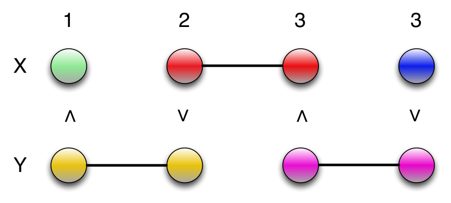
Refer to caption
Fig. 4: Coloring the characteristic graph under the optimal function with N=3N=3 and L=4L=4
Refer to caption
Fig. 5: Coloring the characteristic graph under the optimal function with N=2N=2 and L=4L=4

For the case that N=2N=2, since there will be LL different ties that need to be distinguished, and 2L2^{L} different candidate functions that need to be considered, we have:

Corollary 1 (N=2N=2 case).

Among all 2L2^{L} arg​max\argmax functions, the one that achieves the lowest sum-rate under minimum entropy graph coloring satisfies the property that for all αi∈𝒳\alpha_{i}\in\mathcal{X},

f2∗​(αi,αi)={1,i odd2,i even.f^{*}_{2}(\alpha_{i},\alpha_{i})=\begin{cases}1,&$i$ odd\\ 2,&$i$ even.\\ \end{cases} (33)
Refer to caption
Fig. 6: Coloring the characteristic graph under the non-recursive optimal function with N=3N=3 and L=4L=4
Remark.

Another type of candidate arg​max\argmax function which leads to the complement characteristic graph as shown in Fig. 6 with rate

R⁡(fN∗)=(N−2)​H​(X)+minc1∈𝒞⁡(G1​(f2∗))⁡H⁡(c1​(X1))+minc2∈𝒞⁡(G2​(f2∗))⁡H⁡(c2​(X2))R(f_{N}^{*})=(N-2)H(X)+\min_{c_{1}\in\mathcal{C}(G_{1}(f^{*}_{2}))}H(c_{1}(X_{1}))+\min_{c_{2}\in\mathcal{C}(G_{2}(f^{*}_{2}))}H(c_{2}(X_{2})) (34)

although do not have the recursive property, can still achieve (28), and this structure can be interpreted as 22 of the NN users do graph coloring by Corollary 1, and the rest of the N−2N-2 users Huffman encode their own sources.

Having introduced this scheme, we will show in the next section that no scheme can have a higher rate-savings than this one.

IV-B Converse of Determining the Extremization Functions

The following lemma is necessary to aid in drawing the conclusion that joint graph coloring achieves the fundamental limit and there is no benefit from the OR-product graph for arg​max\argmax.

Lemma 4.

For any given candidate arg​max\argmax function fN∈ℱA,Nf_{N}\in\mathcal{F}_{A,N}, the conditional probability p⁡(w|x)p(w|x), which is supported on the maximal independent sets ww containing the vertices xx, to achieve the minimum mutual information in the graph entropy expression (15) must be either 11 or 00 for all n∈[N]n\in[N].

Proof: We prove this by showing that no vertex exists in two different maximal independent sets. Without loss of generality, we consider vertex αi\alpha_{i} in X1X_{1}’s characteristic graph. By Lemma 2, the two maximal independent sets that αi\alpha_{i} may belong to are w1={αi−1,αi}w_{1}=\{\alpha_{i-1},\alpha_{i}\} and w2={αi,αi+1}w_{2}=\{\alpha_{i},\alpha_{i+1}\}. If vertex αi∈w1\alpha_{i}\in w_{1} under the arg​max\argmax function fNf_{N} (which means there is no edge between αi−1\alpha_{i-1} and αi\alpha_{i}), then ∀𝒙∖{1}∈𝒳N−1\forall\bm{x}_{\setminus\{1\}}\in\mathcal{X}^{N-1}, we have

fN​(αi,𝒙∖{1})=fN​(αi−1,𝒙∖{1}).f_{N}(\alpha_{i},\bm{x}_{\setminus\{1\}})=f_{N}(\alpha_{i-1},\bm{x}_{\setminus\{1\}}). (35)

In particular, there exists 𝒙∖{1}=(αi,αi−1,…,αi−1)\bm{x}_{\setminus\{1\}}=(\alpha_{i},\alpha_{i-1},\ldots,\alpha_{i-1}) such that

fN​(αi,𝒙∖{1})=fN​(αi−1,𝒙∖{1})=2,f_{N}(\alpha_{i},\bm{x}_{\setminus\{1\}})=f_{N}(\alpha_{i-1},\bm{x}_{\setminus\{1\}})=2, (36)

and obviously

fN​(αi+1,𝒙∖{1})=1.f_{N}(\alpha_{i+1},\bm{x}_{\setminus\{1\}})=1. (37)

Therefore, x1=αix_{1}=\alpha_{i} is connected to x1=αi+1x_{1}=\alpha_{i+1}, and the set w2={αi,αi+1}w_{2}=\{\alpha_{i},\alpha_{i+1}\} is not an independent set in X1X_{1}’s characteristic graph, and we have

p⁡(w|x1=αi)={1,w={αi−1,αi}0,otherwise.p(w|x_{1}=\alpha_{i})=\begin{cases}1,&$w=\{\alpha_{i-1},\alpha_{i}\}$\\ 0,&otherwise.\\ \end{cases} (38)

■\blacksquare

Theorem 3.

To losslessly determine the arg​max\argmax, the fundamental limit of the sum-rate can be achieved by coloring the characteristic graph of each user, hence the OR-product graph is not necessary.

Proof:

As reviewed at (16), the fundamental limit of the sum-rate with independent sources problems is the sum of the graph entropy, i.e. RA∗=∑n=1NRnR_{A}^{*}=\sum_{n=1}^{N}R_{n} with Rn=HG​(Xn)R_{n}=H_{G}(X_{n}). By Lemma 4, for any given candidate arg​max\argmax function,

HG​(Xn)\displaystyle H_{G}(X_{n}) =minp⁡(wn|xn)∈{0,1},wn∈Γ⁡(Gn)⁡I⁡(Wn,Xn)\displaystyle=\min_{p(w_{n}|x_{n})\in\{0,1\},w_{n}\in\Gamma(G_{n})}I(W_{n};X_{n}) (39)
=minp⁡(wn|xn)∈{0,1},wn∈Γ⁡(Gn)⁡H⁡(Wn)−H⁡(Wn|Xn)\displaystyle=\min_{p(w_{n}|x_{n})\in\{0,1\},w_{n}\in\Gamma(G_{n})}H(W_{n})-H(W_{n}|X_{n})
=minp⁡(wn|xn)∈{0,1},wn∈Γ⁡(Gn)⁡H⁡(Wn).\displaystyle=\min_{p(w_{n}|x_{n})\in\{0,1\},w_{n}\in\Gamma(G_{n})}H(W_{n}).

Note that the proof of Lemma 4 implies that the maximal independent sets are disjoint, and the fact that one can always Huffman encode the maximal independent sets with any given distribution. Consider using colors to represent the maximal independent sets, then Huffman encode the sets is the same as Huffman encode these colors. This color representation is a normal coloring method w.r.t. the characteristic graph since any two vertices connected by an edge will be in two different independent sets and no two maximal independent sets share the same color. Also note that when the maximal independents are disjoint, distinguish the vertices in the same independent set will result in a higher mutual information in the graph entropy optimization, since for any probabilities pip_{i}, pi+1p_{i+1} of the the nodes in a pairwise maximal independent set {αi,αi+1}\{\alpha_{i},\alpha_{i+1}\}, the difference of the mutual information will be

−pi​log2​pi−pi+1​log2​pi+1+(pi+pi+1)​log2⁡(pi+pi+1)\displaystyle-p_{i}\log_{2}p_{i}-p_{i+1}\log_{2}p_{i+1}+(p_{i}+p_{i+1})\log_{2}(p_{i}+p_{i+1}) =−pi​log2⁡(pipi+pi+1)−pi+1​log2⁡(pi+1pi+pi+1)\displaystyle=-p_{i}\log_{2}\left(\frac{p_{i}}{p_{i}+p_{i+1}}\right)-p_{i+1}\log_{2}\left(\frac{p_{i+1}}{p_{i}+p_{i+1}}\right) (40)
=(pi+pi+1)​h2​(pipi+pi+1)≥0\displaystyle=\left(p_{i}+p_{i+1}\right)h_{2}(\frac{p_{i}}{p_{i}+p_{i+1}})\geq 0

where h2​()h_{2}() is the binary entropy function. Therefore (39) can be achieved by graph coloring. Since the scheme we present in Theorem 2 is the optimal coloring method w.r.t. the non-product characteristic graph, it must achieve the minimum in (39). Therefore we have the following relationship for all n∈[N]n\in[N] and the fundamental limit of the sum-rate can be achieved by Theorem 2.

HG​(Xn)​≤(a)​limS→∞1S​mincn∈𝒞ϵ​(GnS​(f))⁡H⁡(cn​(Xn))​≤(b)​mincn∈𝒞⁡(Gn​(f))⁡H⁡(cn​(Xn))​=(c)​HG​(Xn)H_{G}(X_{n})\overset{(a)}{\leq}\lim_{S\rightarrow\infty}\frac{1}{S}\min_{c_{n}\in\mathcal{C_{\epsilon}}(G_{n}^{S}(f))}H(c_{n}(X_{n}))\overset{(b)}{\leq}\min_{c_{n}\in\mathcal{C}(G_{n}(f))}H(c_{n}(X_{n}))\overset{(c)}{=}H_{G}(X_{n}) (41)

where (a) holds by [42]; (b) holds by achievability: an ordinary coloring is also an ϵ\epsilon-coloring, and a valid ordinary coloring on the characteristic graph can be used in replication to achieve a valid coloring on the OR-product graph; and we have proved (c) above. ∎

We now give the fundamental limit of the sum-rate in the problem that the CEO needs to determine ZMZ_{M} and ZA,MZ_{A,M} respectively.

Definition 4.

A function f:𝒳N→𝒳f:\mathcal{X}^{N}\rightarrow\mathcal{X} is a candidate max\max function if and only if

𝔼⁡[dM​((X1,…,XN),f⁡(X1,…,XN))]=0.\mathbb{E}[d_{M}((X_{1},\ldots,X_{N}),f(X_{1},\ldots,X_{N}))]=0. (42)

Let ℱM,N\mathcal{F}_{M,N} be the set of all such candidate max\max functions with NN inputs. For any f∈ℱM,Nf\in\mathcal{F}_{M,N}, it indicates the max\max.

Definition 5.

A function f:𝒳N→{1,…,N}×𝒳f:\mathcal{X}^{N}\rightarrow\{1,\ldots,N\}\times\mathcal{X} is a candidate (arg​max,max)(\argmax,\max) function if and only if

𝔼⁡[dA,M​((X1,…,XN),f⁡(X1,…,XN))]=0.\mathbb{E}[d_{A,M}((X_{1},\ldots,X_{N}),f(X_{1},\ldots,X_{N}))]=0. (43)

Let ℱP,N\mathcal{F}_{P,N} be the set of all such candidate (arg​max,max)(\argmax,\max) functions with NN inputs. For any f∈ℱP,Nf\in\mathcal{F}_{P,N}, it indicates both the index of a user attaining the max\max and the max\max.

Theorem 4.

In the problem that the CEO needs to decide Z^M\hat{Z}_{M}, if min⁡𝒳>0\min\mathcal{X}>0, then the minimum sum-rate will be

RM∗=∑n=1NH⁡(Xn).R_{M}^{*}=\sum_{n=1}^{N}H(X_{n}). (44)
Proof:

The distortion measure dMd_{M} is

dM​((X1,s,…,XN,s),Z^M​(s))={ZM​(s)−Z^M​(s)if Z^M​(s)≤ZM​(s)ZM​(s)otherwise.d_{M}((X_{1,s},\ldots,X_{N,s}),\hat{Z}_{M}(s))=\begin{cases}Z_{M}(s)-\hat{Z}_{M}(s)&if $\hat{Z}_{M}(s)\leq Z_{M}(s)$\\ Z_{M}(s)&otherwise.\end{cases} (45)

Given min⁡𝒳>0\min\mathcal{X}>0, ZM​(s)Z_{M}(s) can never be 00, the only way to make (42) happen is to let Z^M​(s)\hat{Z}_{M}(s) exactly estimate ZM​(s)Z_{M}(s), in other words, (42) is satisfied if and only if

f⁡(X1,s,…,XN,s)=max⁡(X1,s,…,XN,s).f(X_{1,s},\ldots,X_{N,s})=\max(X_{1,s},\ldots,X_{N,s}). (46)

For any node pair (αi\alpha_{i}, αj\alpha_{j}) in user nn’s characteristic graph, assume i<ji<j w.l.o.g., we will have (αi,αj)∈Gn(\alpha_{i},\alpha_{j})\in G_{n} since there exists 𝒙∖{n}=(αi,…,αi)\bm{x}_{\setminus\{n\}}=(\alpha_{i},\ldots,\alpha_{i}) such that

f⁡(αi,𝒙∖{n})≠f⁡(αj,𝒙∖{n}).f(\alpha_{i},\bm{x}_{\setminus\{n\}})\neq f(\alpha_{j},\bm{x}_{\setminus\{n\}}). (47)

Therefore, the characteristic graph of user nn w.r.t. ff is complete, and Γ⁡(Gn)={{αi}:αi∈𝒳}\Gamma(G_{n})=\{\{\alpha_{i}\}:\alpha_{i}\in\mathcal{X}\}, and the graph entropy is the same as the entropy of each source. ∎

Remark.

To achieve this limit, we simply need each user to Huffman encode its source.

Corollary 2.

In the problem that the CEO needs to decide (Z^A,Z^M)(\hat{Z}_{A},\hat{Z}_{M}), if min⁡𝒳>0\min\mathcal{X}>0, then the minimum sum-rate will be

RA,M∗=∑n=1NH⁡(Xn).R_{A,M}^{*}=\sum_{n=1}^{N}H(X_{n}). (48)
Proof:

This directly follows the proof of Theorem 4, the characteristic graph is also complete if min⁡𝒳>0\min\mathcal{X}>0. ∎

Theorem 5.

In the problem that the CEO needs to decide Z^M\hat{Z}_{M}, if min⁡𝒳=0\min\mathcal{X}=0, then the minimum sum-rate satisfies

RM∗\displaystyle R_{M}^{*} =N​H​(X)+N⁡(p1​log2​p1+p2​log2​p2−(p1+p2)​log2⁡(p1+p2))\displaystyle=NH(X)+N\left(p_{1}\log_{2}p_{1}+p_{2}\log_{2}p_{2}-\left(p_{1}+p_{2}\right)\log_{2}\left(p_{1}+p_{2}\right)\right) (49)
=N​H​(X)−N⁡(p1+p2)​h2​(p1p1+p2)\displaystyle=NH(X)-N\left(p_{1}+p_{2}\right)h_{2}\left(\frac{p_{1}}{p_{1}+p_{2}}\right)

where p1=ℙ⁡(X=α1=0)p_{1}=\mathbb{P}(X=\alpha_{1}=0) and p2=ℙ⁡(X=α2)p_{2}=\mathbb{P}(X=\alpha_{2}).

Proof:

Let f∈ℱM,Nf\in\mathcal{F}_{M,N} satisfies that f⁡(α1,…,α1)=α2f(\alpha_{1},\ldots,\alpha_{1})=\alpha_{2}, then (α1,α2)∉G(\alpha_{1},\alpha_{2})\not\in G for the characteristic graph of each source XiX_{i} w.r.t. ff. The graph is not complete and the set of independent sets is Γ⁡(Gn)={{α1,α2},{α3},…,{αL}}\Gamma(G_{n})=\{\{\alpha_{1},\alpha_{2}\},\{\alpha_{3}\},\ldots,\{\alpha_{L}\}\} for all n∈[N]n\in[N]. Hence by a similar proof as in Theorem 2 and Theorem 3, we have

RM∗=∑n=1NHG​(Xn)R_{M}^{*}=\sum_{n=1}^{N}H_{G}(X_{n}) (50)

with

HG​(Xn)=−(p1+p2)​log2⁡(p1+p2)−∑i=3Lpi​log2​piH_{G}(X_{n})=-\left(p_{1}+p_{2}\right)\log_{2}\left(p_{1}+p_{2}\right)-\sum_{i=3}^{L}p_{i}\log_{2}p_{i} (51)

for all n∈[N]n\in[N]. ∎

Theorem 6.

In the problem that the CEO needs to decide (Z^A,Z^M)(\hat{Z}_{A},\hat{Z}_{M}), if min⁡𝒳=0\min\mathcal{X}=0, then the minimum sum-rate satisfies

RA,M∗\displaystyle R_{A,M}^{*} =N​H​(X)+(p1​log2​p1+p2​log2​p2−(p1+p2)​log2⁡(p1+p2))\displaystyle=NH(X)+\left(p_{1}\log_{2}p_{1}+p_{2}\log_{2}p_{2}-\left(p_{1}+p_{2}\right)\log_{2}\left(p_{1}+p_{2}\right)\right) (52)
=N​H​(X)−(p1+p2)​h2​(p1p1+p2)\displaystyle=NH(X)-\left(p_{1}+p_{2}\right)h_{2}\left(\frac{p_{1}}{p_{1}+p_{2}}\right)

where p1=ℙ⁡(X=α1)=ℙ⁡(X=0)p_{1}=\mathbb{P}(X=\alpha_{1})=\mathbb{P}(X=0) and p2=ℙ⁡(X=α2)p_{2}=\mathbb{P}(X=\alpha_{2}).

Proof:

Let f=(fA,fM)∈ℱP,Nf=(f_{A},f_{M})\in\mathcal{F}_{P,N}. Note that (43) is satisfied if and only if both (22) and (42) are satisfied, and hence {αi,αj}∉Gn\{\alpha_{i},\alpha_{j}\}\not\in G_{n} in user nn’s characteristic graph if and only if fA​(αi,𝒙∖{n})=fA​(αj,𝒙∖{n})f_{A}(\alpha_{i},\bm{x}_{\setminus\{n\}})=f_{A}(\alpha_{j},\bm{x}_{\setminus\{n\}}) and fM​(αi,𝒙∖{n})=fM​(αj,𝒙∖{n})f_{M}(\alpha_{i},\bm{x}_{\setminus\{n\}})=f_{M}(\alpha_{j},\bm{x}_{\setminus\{n\}}) for all 𝒙∖{n}=(xk|k∈[N]∖{n},xk∈𝒳)\bm{x}_{\setminus\{n\}}=(x_{k}|k\in[N]\setminus\{n\},x_{k}\in\mathcal{X}). Let fA∈ℱA,Nf_{A}\in\mathcal{F}_{A,N} be defined as in Theorem 2 and fM∈ℱM,Nf_{M}\in\mathcal{F}_{M,N} as in Theorem 5, then {α1,α2}∉G1\{\alpha_{1},\alpha_{2}\}\not\in G_{1}, and all characteristic graphs other than G1G_{1} are complete. The sets of independent sets are Γ⁡(G1)={{α1,α2},{α3},…,{αL}}\Gamma(G_{1})=\{\{\alpha_{1},\alpha_{2}\},\{\alpha_{3}\},\ldots,\{\alpha_{L}\}\}, and Γ⁡(Gn)={{α1},{α2},…,{αL}}\Gamma(G_{n})=\{\{\alpha_{1}\},\{\alpha_{2}\},\ldots,\{\alpha_{L}\}\} for all n∈[N]∖{1}n\in[N]\setminus\{1\}. By a similar proof as in Theorem 2 and Theorem 3, we have

RA,M∗=∑n=1NHG​(Xn)R_{A,M}^{*}=\sum_{n=1}^{N}H_{G}(X_{n}) (53)

with

HG​(X1)=−(p1+p2)​log2⁡(p1+p2)−∑i=3Lpi​log2​piH_{G}(X_{1})=-\left(p_{1}+p_{2}\right)\log_{2}\left(p_{1}+p_{2}\right)-\sum_{i=3}^{L}p_{i}\log_{2}p_{i} (54)

and

HG​(Xn)=H⁡(X)H_{G}(X_{n})=H(X) (55)

for all n∈[N]∖{1}n\in[N]\setminus\{1\}. ∎

IV-C Scaling in Number of Users

In this subsection, we consider the rate saving performance of graph coloring in a large scale of NN. Define the rate savings as the difference between the scheme that each user Huffman encode its source and the scheme by Theorem 2, i.e.

ΔA≜∑n=1NH⁡(Xn)−RA∗.\Delta_{A}\triangleq\sum_{n=1}^{N}H(X_{n})-R_{A}^{*}. (56)
Theorem 7.

To losslessly determine the arg​max\argmax, the savings ΔA\Delta_{A} is bounded by

maxp1,…,pL⁡ΔA=max⁡∑i=1L−1p1,…,pL⁡(pi+pi+1)​h2​(pipi+pi+1)≤2\max_{p_{1},\ldots,p_{L}}\Delta_{A}=\max_{p_{1},\ldots,p_{L}}\sum_{i=1}^{L-1}\left(p_{i}+p_{i+1}\right)h_{2}\left(\frac{p_{i}}{p_{i}+p_{i+1}}\right)\leq 2 (57)

where pi=ℙ⁡(X=αi)p_{i}=\mathbb{P}(X=\alpha_{i}), and hence the per user saving satisfies that

limN→∞ΔAN=0.\lim_{N\rightarrow\infty}\frac{\Delta_{A}}{N}=0. (58)
Proof:

See Appendix -A2 ∎

Corollary 3.

In the problem that the CEO needs to decide the m​a​xmax, the per user saving ΔM/N\nicefrac{{\Delta_{M}}}{{N}} satisfies

limN→∞ΔMN={0if min⁡𝒳>0−(p1+p2)​h2​(p1p1+p2)if min⁡𝒳=0\lim_{N\rightarrow\infty}\frac{\Delta_{M}}{N}=\begin{cases}0&if $\min\mathcal{X}>0$\\ -\left(p_{1}+p_{2}\right)h_{2}\left(\frac{p_{1}}{p_{1}+p_{2}}\right)&if $\min\mathcal{X}=0$\end{cases} (59)

where p1=ℙ⁡(x=α1)=ℙ⁡(x=0)p_{1}=\mathbb{P}(x=\alpha_{1})=\mathbb{P}(x=0) and p2=ℙ⁡(x=α2)p_{2}=\mathbb{P}(x=\alpha_{2}).

Proof:

See Appendix -A3 ∎

Corollary 4.

In the problem that the CEO needs to decide the pair (arg​max,max)(\argmax,\max), the per user saving ΔA,M/N\nicefrac{{\Delta_{A,M}}}{{N}} goes to 00 as NN goes to infinity.

Proof:

Observe that

RA∗≤RA,M∗≤∑n=1NH⁡(Xn).R_{A}^{*}\leq R_{A,M}^{*}\leq\sum_{n=1}^{N}H(X_{n}). (60)

∎As we shall see in Section VI, the lack of savings in this lossless non-interactive problem structure stands in stark contrast to an interactive setup in which it can be shown that, by allowing the CEO to communicate with the users over multiple rounds, a substantial saving in sum rate relative to the the non-interactive scheme can be achieved [43] while still obtaining the answer losslessly. Additionally, as we will see in Section V, substantial rate savings can be obtained if we are willing to tolerate a small amount of loss.

V Lossy Extremization

In the previous section, it was shown that having a CEO losslessly compute the max\max, arg​max\argmax, or (max,arg​max)(\max,\argmax) of a set of distributed sources does not result in a significant rate savings relative to simply recovering all of the sources. For applications where reducing the rate is critical, tolerating bounded estimation error may be necessary. In this section, we consider the lossy variant of the function computation problem where the CEO need not determine the function output exactly. In particular, we first bound the best achievable rate-distortion tradeoff by computing the rate-distortion curves for each of the three functions with an adapted version of the Blahut-Arimoto algorithm in Section V-A. Achievable schemes for each of the three functions based on scalar quantization followed by entropy encoding are then presented in Section V-B and Section V-C. For certain problem instances, this scheme closely approximates the rate-distortion function as shown in Section V-D.

V-A Fundamental Limits—Multi-Source Blahut-Arimoto

In this subsection, we first utilize a generalized BA (BA) algorithm to compute the sum-rate distortion function for the independent CEO extremization problems with discrete sources. We then show by Theorem 8 and Corollary 5 that the sum-rate distortion function for the case of continuous sources can be well approximated by discretizing the sources and applying the generalized BA algorithm from [33] to compute the rate distortion function for the discretized sources. In the limit as the discretization becomes arbitrarily fine, the discretized rate distortion function provides an ϵ\epsilon-lower bound for the continuous one. This calculated lower bound is used in Section V-D to measure the performance of the continuous quantizations we propose in Section V-B and Section V-C.

We first prove our discretization result for the classical single-source rate distortion function for continuous sources with bounded support.

Theorem 8.

For any continuous source XX with bounded support set 𝒳=(xm​i​n,xm​a​x)\mathcal{X}=(x_{min},x_{max}) and bounded PDF f⁡(x)f(x) if there exists a continuous quantizer

𝑸:𝒳S→{1,…,2S​R}\bm{Q}:\mathcal{X}^{S}\rightarrow\{1,\ldots,2^{SR}\} (61)

a reconstruction function

g:{1,…,2S​R}→𝒳^={𝒙^1,…,𝒙^L}g:\{1,\ldots,2^{SR}\}\rightarrow\hat{\mathcal{X}}=\{\bm{\hat{x}}_{1},\ldots,\bm{\hat{x}}_{L}\} (62)

and a distortion metric

d:𝒳×𝒳^→R+d:\mathcal{X}\times\hat{\mathcal{X}}\rightarrow R^{+} (63)

that attain rate distortion pair (R,D)(R,D), where

L=2S​RL=2^{SR} (64)
𝒙^ℓ=(x^ℓ,1,…,x^ℓ,S)\bm{\hat{x}}_{\ell}=\left(\hat{x}_{\ell,1},\ldots,\hat{x}_{\ell,S}\right) (65)
D=𝔼⁡[𝒅⁡(𝑿,𝑿^ℓ)]D=\mathbb{E}[\bm{d}(\bm{X},\bm{\hat{X}}_{\ell})] (66)
𝒅⁡(𝒙,𝒙^ℓ)=1S​∑s=1Sd⁡(xs,x^ℓ,s)\bm{d}(\bm{x},\bm{\hat{x}}_{\ell})=\frac{1}{S}\sum_{s=1}^{S}d(x_{s},\hat{x}_{\ell,s}) (67)

with d⁡(⋅)d(\cdot) bounded above by dmd_{m}, and, when regarded as a function of 𝐱\bm{x} for a fixed 𝐱^ℓ\bm{\hat{x}_{\ell}}, 𝐝⁡(𝐱,𝐱^ℓ)\bm{d}(\bm{x},\bm{\hat{x}}_{\ell}) has at most a finite number of discontinuous points, then there must exist a discrete source YKY_{K}, a discrete quantizer

𝑸Kd:𝒴KS→{1,…,2S​R}\bm{Q}^{d}_{K}:\mathcal{Y}_{K}^{S}\rightarrow\{1,\ldots,2^{SR}\} (68)

along with the same distortion metric dd and reconstruction mapping gg that attains rate RK=RR_{K}=R and distortion DK≥DD_{K}\geq D, where YK=QK​(X)Y_{K}=Q_{K}(X) is built by uniformly quantizing XX into KK intervals with the reconstruction levels 𝒴K={uk:k∈[K]}\mathcal{Y}_{K}=\{u_{k}:k\in[K]\}. Further, DKD_{K} can be arbitrarily close to DD for a large enough KK, i.e.

limK→∞DK=D\lim_{K\rightarrow\infty}D_{K}=D (69)
Proof:

Given a continuous source XX with 𝒳=[xm​i​n,xm​a​x]\mathcal{X}=[x_{min},x_{max}] and PDF f⁡(x)f(x), the expected distortion is

D\displaystyle D =𝔼⁡[𝒅⁡(𝑿,𝑿^)]\displaystyle=\mathbb{E}[\bm{d}(\bm{X},\bm{\hat{X}})] (70)
=∫𝒅⁡(𝒙,𝑸⁡(𝒙))​f​(𝒙)​𝒅𝒙\displaystyle=\int\bm{d}(\bm{x},\bm{Q}(\bm{x}))f(\bm{x})d\bm{x}

where we denote 𝒙^ℓ=g⁡(𝑸⁡(𝒙))\bm{\hat{x}}_{\ell}=g(\bm{Q}(\bm{x})) by 𝑸⁡(𝒙)\bm{Q}(\bm{x}) for convenience, and

𝒅⁡(𝒙,𝑸⁡(𝒙))=1S​∑s=1Sd⁡(xs,(𝑸⁡(𝒙))s)\bm{d}(\bm{x},\bm{Q}(\bm{x}))=\frac{1}{S}\sum_{s=1}^{S}d\left(x_{s},\left(\bm{Q}(\bm{x})\right)_{s}\right) (71)

Now let QKQ_{K} that uniformly quantizes XX with KK intervals, i.e.

QK:𝒳→{ℐk:k∈[K]}Q_{K}:\mathcal{X}\rightarrow\{\mathcal{I}_{k}:k\in[K]\} (72)

where

ℐk=(xm​i​n+k−1K​(xm​a​x−xm​i​n),xm​i​n+kK​(xm​a​x−xm​i​n)).\mathcal{I}_{k}=(x_{min}+\frac{k-1}{K}\left(x_{max}-x_{min}\right),\ x_{min}+\frac{k}{K}\left(x_{max}-x_{min}\right)). (73)

Let gKg_{K} that maps the intervals to the reconstruction levels, i.e.

gK:{ℐk:k∈K}→{uk:k∈[K]}g_{K}:\{\mathcal{I}_{k}:k\in K\}\rightarrow\{u_{k}:k\in[K]\} (74)

with

uk=a​r​g​minx∈ℐk​d​(x,Q⁡(x)).u_{k}=\underset{x\in\mathcal{I}_{k}}{arg\min}\;d(x,Q(x)). (75)

The discrete random variable YKY_{K} by discretizing XX is then defined on the support set

𝒴K={uk:k∈[K]}\mathcal{Y}_{K}=\{u_{k}:k\in[K]\} (76)

with PMF

ℙ[YK=uk]=∫x∈ℐkf(x)dx.\mathbb{P}[Y_{K}=u_{k}]=\int_{x\in\mathcal{I}_{k}}f(x)dx. (77)

Let 𝒚K=(yK,s:s∈[S])\bm{y}_{K}=\left(y_{K,s}:s\in[S]\right), the discrete quantizer 𝑸Kd\bm{Q}^{d}_{K} satisfies

𝑸Kd​(𝒚K)=𝑸⁡(𝒚K).\bm{Q}^{d}_{K}(\bm{y}_{K})=\bm{Q}(\bm{y}_{K}). (78)

The distortion DKD_{K} for quantization QKdQ^{d}_{K} will be

DK=𝔼[𝒅(𝒀K,𝑸Kd(𝒀K)]=∑𝒚K∈𝒴KS𝒅(𝒚K,𝑸Kd(𝒚K))ℙ[𝒀K=𝒚K]D_{K}=\mathbb{E}[\bm{d}(\bm{Y}_{K},\bm{Q}^{d}_{K}(\bm{Y}_{K})]=\sum_{\bm{y}_{K}\in\mathcal{Y}_{K}^{S}}\bm{d}(\bm{y}_{K},\bm{Q}^{d}_{K}(\bm{y}_{K}))\mathbb{P}[\bm{Y}_{K}=\bm{y}_{K}] (79)

where

𝒅⁡(𝒚K,𝑸Kd​(𝒚K))=1S​∑s=1Sd⁡(yK,s,(𝑸Kd​(𝒚K))s).\bm{d}(\bm{y}_{K},\bm{Q}^{d}_{K}(\bm{y}_{K}))=\frac{1}{S}\sum_{s=1}^{S}d\left(y_{K,s},\left(\bm{Q}^{d}_{K}(\bm{y}_{K})\right)_{s}\right). (80)

Let 𝑸K​(⋅)\bm{Q}_{K}(\cdot) quantize 𝒙\bm{x} element wise as QKQ_{K} does. In addition, let

ℐ⁡(𝒚K)={𝒙∈𝒳S|𝑸K​(𝒙)=𝒚K}=ℐ1​(𝒚K)∪ℐ2​(𝒚K)∪ℐ3​(𝒚K)\mathcal{I}(\bm{y}_{K})=\{\bm{x}\in\mathcal{X}^{S}|\bm{Q}_{K}(\bm{x})=\bm{y}_{K}\}=\mathcal{I}_{1}(\bm{y}_{K})\cup\mathcal{I}_{2}(\bm{y}_{K})\cup\mathcal{I}_{3}(\bm{y}_{K}) (81)

be a subset of 𝒳S\mathcal{X}^{S} that maps to 𝒚K\bm{y}_{K} by 𝑸K​(⋅)\bm{Q}_{K}(\cdot), where

ℐ1​(𝒚K)={ℐ⁡(𝒚K)if 𝑸⁡(𝒙)=𝑸⁡(𝒚K) for all 𝒙∈ℐ⁡(𝒚K) and 𝒅⁡(𝒙,𝒙^) is continuous on ℐ⁡(𝒚K)∅otherwise\mathcal{I}_{1}(\bm{y}_{K})=\begin{cases}\mathcal{I}(\bm{y}_{K})&if $\bm{Q}(\bm{x})=\bm{Q}(\bm{y}_{K})$ for all $\bm{x}\in\mathcal{I}(\bm{y}_{K})$ and $\bm{d}(\bm{x},\bm{\hat{x}})$ is continuous on $\mathcal{I}(\bm{y}_{K})$\\ \emptyset&otherwise\end{cases} (82)
ℐ2​(𝒚K)={ℐ⁡(𝒚K)if 𝑸⁡(𝒙)=𝑸⁡(𝒚K) for all 𝒙∈ℐ⁡(𝒚K) and 𝒅⁡(𝒙,𝒙^) is not continuous on ℐ⁡(𝒚K)∅otherwise\mathcal{I}_{2}(\bm{y}_{K})=\begin{cases}\mathcal{I}(\bm{y}_{K})&if $\bm{Q}(\bm{x})=\bm{Q}(\bm{y}_{K})$ for all $\bm{x}\in\mathcal{I}(\bm{y}_{K})$ and $\bm{d}(\bm{x},\bm{\hat{x}})$ is not continuous on $\mathcal{I}(\bm{y}_{K})$\\ \emptyset&otherwise\end{cases} (83)

and

ℐ3​(𝒚K)={ℐ⁡(𝒚K)if ∃𝒙1,𝒙2∈ℐ⁡(𝒚K) such that 𝑸⁡(𝒙1)≠𝑸⁡(𝒙2)∅otherwise\mathcal{I}_{3}(\bm{y}_{K})=\begin{cases}\mathcal{I}(\bm{y}_{K})&if $\exists\bm{x}_{1},\bm{x}_{2}\in\mathcal{I}(\bm{y}_{K})$ such that $\bm{Q}(\bm{x}_{1})\neq\bm{Q}(\bm{x}_{2})$\\ \emptyset&otherwise\end{cases} (84)

Clearly, ℐi​(𝒚K)∩ℐj​(𝒚K)=∅\mathcal{I}_{i}(\bm{y}_{K})\cap\mathcal{I}_{j}(\bm{y}_{K})=\emptyset for any i≠j,i,j∈{1,2,3}i\neq j,\ i,j\in\{1,2,3\}. By comparing (70) and (79), we have

D\displaystyle D =∫𝒅⁡(𝒙,𝑸⁡(𝒙))​f​(𝒙)​𝒅𝒙\displaystyle=\int\bm{d}(\bm{x},\bm{Q}(\bm{x}))f(\bm{x})d\bm{x} (85)
=∑𝒚K∈𝒴KS∫𝒙∈ℐ⁡(𝒚K)𝒅⁡(𝒙,𝑸⁡(𝒙))​f​(𝒙)​𝒅𝒙\displaystyle=\sum_{\bm{y}_{K}\in\mathcal{Y}_{K}^{S}}\int_{\bm{x}\in\mathcal{I}(\bm{y}_{K})}\bm{d}(\bm{x},\bm{Q}(\bm{x}))f(\bm{x})d\bm{x}
=∑𝒚K∈𝒴KS∫𝒙∈ℐ⁡(𝒚K)[𝒅⁡(𝒙,𝑸⁡(𝒙))+𝒅⁡(𝒚K,𝑸⁡(𝒚K))−𝒅⁡(𝒚K,𝑸⁡(𝒚K))]​f​(𝒙)​𝒅𝒙\displaystyle=\sum_{\bm{y}_{K}\in\mathcal{Y}_{K}^{S}}\int_{\bm{x}\in\mathcal{I}(\bm{y}_{K})}\left[\bm{d}(\bm{x},\bm{Q}(\bm{x}))+\bm{d}(\bm{y}_{K},\bm{Q}(\bm{y}_{K}))-\bm{d}(\bm{y}_{K},\bm{Q}(\bm{y}_{K}))\right]f(\bm{x})d\bm{x}
=DK+∑𝒚K∈𝒴KS∫𝒙∈ℐ⁡(𝒚K)[𝒅⁡(𝒙,𝑸⁡(𝒙))−𝒅⁡(𝒚K,𝑸⁡(𝒚K))]​f​(𝒙)​𝒅𝒙\displaystyle=D_{K}+\sum_{\bm{y}_{K}\in\mathcal{Y}_{K}^{S}}\int_{\bm{x}\in\mathcal{I}(\bm{y}_{K})}\left[\bm{d}(\bm{x},\bm{Q}(\bm{x}))-\bm{d}(\bm{y}_{K},\bm{Q}(\bm{y}_{K}))\right]f(\bm{x})d\bm{x}

First observe by (71) and (75) that

D=DK+∑𝒚K∈𝒴KS∫𝒙∈ℐ⁡(𝒚K)[𝒅⁡(𝒙,𝑸⁡(𝒙))−𝒅⁡(𝒚K,𝑸⁡(𝒚K))]​f​(𝒙)​𝑑𝒙≥DKD=D_{K}+\sum_{\bm{y}_{K}\in\mathcal{Y}_{K}^{S}}\int_{\bm{x}\in\mathcal{I}(\bm{y}_{K})}\left[\bm{d}(\bm{x},\bm{Q}(\bm{x}))-\bm{d}(\bm{y}_{K},\bm{Q}(\bm{y}_{K}))\right]f(\bm{x})d\bm{x}\geq D_{K} (86)

then we can further express (85) as

D\displaystyle D =DK+∑𝒚K∈𝒴KS∫𝒙∈ℐ⁡(𝒚K)[𝒅⁡(𝒙,𝑸⁡(𝒙))−𝒅⁡(𝒚K,𝑸⁡(𝒚K))]​f​(𝒙)​𝒅𝒙\displaystyle=D_{K}+\sum_{\bm{y}_{K}\in\mathcal{Y}_{K}^{S}}\int_{\bm{x}\in\mathcal{I}(\bm{y}_{K})}\left[\bm{d}(\bm{x},\bm{Q}(\bm{x}))-\bm{d}(\bm{y}_{K},\bm{Q}(\bm{y}_{K}))\right]f(\bm{x})d\bm{x} (87)
=DK+∑𝒚K∈𝒴KS∫𝒙∈ℐ1​(𝒚K)∪ℐ2​(𝒚K)∪ℐ3​(𝒚K)[𝒅⁡(𝒙,𝑸⁡(𝒙))−𝒅⁡(𝒚K,𝑸⁡(𝒚K))]​f​(𝒙)​𝒅𝒙\displaystyle=D_{K}+\sum_{\bm{y}_{K}\in\mathcal{Y}_{K}^{S}}\int_{\bm{x}\in\mathcal{I}_{1}(\bm{y}_{K})\cup\mathcal{I}_{2}(\bm{y}_{K})\cup\mathcal{I}_{3}(\bm{y}_{K})}\left[\bm{d}(\bm{x},\bm{Q}(\bm{x}))-\bm{d}(\bm{y}_{K},\bm{Q}(\bm{y}_{K}))\right]f(\bm{x})d\bm{x}
=DK+A⁡(ℐ1)+A⁡(ℐ2)+A⁡(ℐ3)\displaystyle=D_{K}+A(\mathcal{I}_{1})+A(\mathcal{I}_{2})+A(\mathcal{I}_{3})

where

A⁡(ℐi)=∑𝒚K∈𝒴KS∫𝒙∈ℐi​(𝒚K)[𝒅⁡(𝒙,𝑸⁡(𝒙))−𝒅⁡(𝒚K,𝑸⁡(𝒚K))]​f​(𝒙)​𝑑𝒙.A(\mathcal{I}_{i})=\sum_{\bm{y}_{K}\in\mathcal{Y}_{K}^{S}}\int_{\bm{x}\in\mathcal{I}_{i}(\bm{y}_{K})}\left[\bm{d}(\bm{x},\bm{Q}(\bm{x}))-\bm{d}(\bm{y}_{K},\bm{Q}(\bm{y}_{K}))\right]f(\bm{x})d\bm{x}. (88)

For any S-fold vector quantization 𝑸⁡(⋅)\bm{Q}(\cdot), we then have the following statements:

  1. (a)

    ∀\forall ϵ1>0\epsilon_{1}>0, ∃\exists a large enough K1K_{1} and a uniform quantization QK1Q_{K_{1}} such that ∀\forall 𝒙∈ℐ1​(𝒚K1)\bm{x}\in\mathcal{I}_{1}(\bm{y}_{K_{1}})

    𝒅⁡(𝒙,𝑸⁡(𝒙))−𝒅⁡(𝒚K1,𝑸⁡(𝒚K1))≤ϵ1\bm{d}(\bm{x},\bm{Q}(\bm{x}))-\bm{d}(\bm{y}_{K_{1}},\bm{Q}(\bm{y}_{K_{1}}))\leq\epsilon_{1} (89)
  2. (b)

    ∀\forall ϵ2>0\epsilon_{2}>0, ∃\exists a large enough K2K_{2} and a uniform quantization QK2Q_{K_{2}} such that

    ∑𝒚K2∈𝒴K2Sℙ[𝑿∈ℐ2(𝒚K2)]<ϵ2.\sum_{\bm{y}_{K_{2}}\in\mathcal{Y}_{K_{2}}^{S}}\mathbb{P}[\bm{X}\in\mathcal{I}_{2}(\bm{y}_{K_{2}})]<\epsilon_{2}. (90)
  3. (c)

    ∀\forall ϵ3>0\epsilon_{3}>0, ∃\exists a large enough K3K_{3} and a uniform quantization QK3Q_{K_{3}} such that

    ∑𝒚K3∈𝒴K3Sℙ[𝑿∈ℐ3(𝒚K3)]<ϵ3.\sum_{\bm{y}_{K_{3}}\in\mathcal{Y}_{K_{3}}^{S}}\mathbb{P}[\bm{X}\in\mathcal{I}_{3}(\bm{y}_{K_{3}})]<\epsilon_{3}. (91)

where (89) holds since d⁡(⋅)d(\cdot) is continuous on ℐ1​(𝒚K)\mathcal{I}_{1}(\bm{y}_{K}); (90) holds since 𝒅⁡(𝒙,𝒙^)\bm{d}(\bm{x},\bm{\hat{x}}) has a finite number (i.e. mm) of discontinuous points on 𝒳S×𝒳^\mathcal{X}^{S}\times\mathcal{\hat{X}}, and for given ϵ=ϵ2/m>0\epsilon=\nicefrac{{\epsilon_{2}}}{{m}}>0, there must exist a large enough K2K_{2} such that when ℐ2​(𝒚K2)≠∅\mathcal{I}_{2}(\bm{y}_{K_{2}})\neq\emptyset,

ℙ[𝑿∈ℐ2(𝒚K2)]<ϵ\mathbb{P}[\bm{X}\in\mathcal{I}_{2}(\bm{y}_{K_{2}})]<\epsilon (92)

hence

∑𝒚K2∈𝒴K2Sℙ[𝑿∈ℐ2(𝒚K2)]\displaystyle\sum_{\bm{y}_{K_{2}}\in\mathcal{Y}_{K_{2}}^{S}}\mathbb{P}[\bm{X}\in\mathcal{I}_{2}(\bm{y}_{K_{2}})] =∑𝒚K2∈𝒴K2S(ℙ⁡[𝑿∈ℐ2​(𝒚K2),ℐ2​(𝒚K2)≠∅]+ℙ⁡[𝑿∈ℐ2​(𝒚K2),ℐ2​(𝒚K2)=∅])\displaystyle=\sum_{\bm{y}_{K_{2}}\in\mathcal{Y}_{K_{2}}^{S}}\left(\mathbb{P}[\bm{X}\in\mathcal{I}_{2}(\bm{y}_{K_{2}}),\mathcal{I}_{2}(\bm{y}_{K_{2}})\neq\emptyset]+\mathbb{P}[\bm{X}\in\mathcal{I}_{2}(\bm{y}_{K_{2}}),\mathcal{I}_{2}(\bm{y}_{K_{2}})=\emptyset]\right) (93)
<m​ϵ+0\displaystyle<m\epsilon+0
=ϵ2.\displaystyle=\epsilon_{2}.

Now we prove (91) also holds. Given a continuous quantizer

𝑸:𝒳S→{1,…,2S​R},\bm{Q}:\mathcal{X}^{S}\rightarrow\{1,\ldots,2^{SR}\}, (94)

a point 𝒙∈𝒳S\bm{x}\in\mathcal{X}^{S} is a boundary point w.r.t. 𝑸\bm{Q} if for any ϵ>0\epsilon>0 there exist 𝒙1∈𝒳S,𝒙1≠𝒙\bm{x}_{1}\in\mathcal{X}^{S},\bm{x}_{1}\neq\bm{x} such that

‖𝒙1−𝒙‖2<ϵ\|\bm{x}_{1}-\bm{x}\|_{2}<\epsilon (95)

and

𝑸⁡(𝒙1)≠𝑸⁡(𝒙).\bm{Q}(\bm{x}_{1})\neq\bm{Q}(\bm{x}). (96)

Let f⁡(𝒙)f(\bm{x}) be a bounded PDF which is defined on 𝒳S⊂ℝS\mathcal{X}^{S}\subset\mathbb{R}^{S} with 𝒳=(xm​i​n,xm​a​x)\mathcal{X}=(x_{min},x_{max}). For a continuous quantizer

𝑸:𝒳S→{1,…,2S​R},\bm{Q}:\mathcal{X}^{S}\rightarrow\{1,\ldots,2^{SR}\}, (97)

let B⁡(𝑸)B(\bm{Q}) be the set of all boundary points w.r.t. 𝑸⁡(⋅)\bm{Q}(\cdot). Since every k-dimensional subspace of ℝS\mathbb{R}^{S} must have measure zero if k<Sk<S, by the definition of measure zero, we have that for any ϵ>0\epsilon>0, there exist open cubes 𝒰1,𝒰2,…\mathcal{U}_{1},\mathcal{U}_{2},\ldots such that B(𝑸)⊆∪i=1∞𝒰iB(\bm{Q})\subseteq\cup_{i=1}^{\infty}\mathcal{U}_{i}, and

∑i=1∞vol⁡(𝒰i)<ϵfm​a​x,\sum_{i=1}^{\infty}\mathrm{vol}(\mathcal{U}_{i})<\frac{\epsilon}{f_{max}}, (98)

where

𝒰i=(ai,1,bi,1)×(ai,2,bi,2)×⋯×(ai,S,bi,S)\mathcal{U}_{i}=(a_{i,1},b_{i,1})\times(a_{i,2},b_{i,2})\times\cdots\times(a_{i,S},b_{i,S}) (99)
vol(𝒰i)=(bi,1−ai,1)(bi,2−ai,2)⋯(bi,S−ai,S)\mathrm{vol}(\mathcal{U}_{i})=(b_{i,1}-a_{i,1})(b_{i,2}-a_{i,2})\cdots(b_{i,S}-a_{i,S}) (100)

and

fm​a​x=max𝒙∈𝒳S⁡f⁡(𝒙).f_{max}=\max_{\bm{x}\in\mathcal{X}^{S}}f(\bm{x}). (101)

Hence

ℙ[𝑿∈∪i=1∞𝒰i]\displaystyle\mathbb{P}[\bm{X}\in\cup_{i=1}^{\infty}\mathcal{U}_{i}] ≤∑i=1∞∫𝒙∈𝒰if⁡(𝒙)​𝒅𝒙\displaystyle\leq\sum_{i=1}^{\infty}\int_{\bm{x}\in\mathcal{U}_{i}}f(\bm{x})d\bm{x} (102)
≤fm​a​x​(∑i=1∞∫𝒙∈𝒰id𝒙)\displaystyle\leq f_{max}\left(\sum_{i=1}^{\infty}\int_{\bm{x}\in\mathcal{U}_{i}}d\bm{x}\right)
=fm​a​x​∑i=1∞vol⁡(𝒰i)\displaystyle=f_{max}\sum_{i=1}^{\infty}\mathrm{vol}(\mathcal{U}_{i})
=ϵ.\displaystyle=\epsilon.

In other words, the boundaries of the quantization levels have probability measure 00.

Therefore, for any ϵ>0\epsilon>0 and any SS, there exists K≥max⁡{K1,K2,K3}K\geq\max\{K_{1},K_{2},K_{3}\} such that

D\displaystyle D =DK+A⁡(ℐ1)+A⁡(ℐ2)+A⁡(ℐ3)\displaystyle=D_{K}+A(\mathcal{I}_{1})+A(\mathcal{I}_{2})+A(\mathcal{I}_{3}) (103)
≤DK+∑𝒚K∈𝓨K∫𝒙∈ℐ1​(𝒚K)ϵ1​f​(𝒙)​𝒅𝒙+∑𝒚K∈𝓨K∫𝒙∈ℐ2​(𝒚K)dm​f​(𝒙)​𝒅𝒙+∑𝒚K∈𝓨K∫𝒙∈ℐ3​(𝒚K)dm​f​(𝒙)​𝒅𝒙\displaystyle\leq D_{K}+\sum_{\bm{y}_{K}\in\bm{\mathcal{Y}}_{K}}\int_{\bm{x}\in\mathcal{I}_{1}(\bm{y}_{K})}\epsilon_{1}f(\bm{x})d\bm{x}+\sum_{\bm{y}_{K}\in\bm{\mathcal{Y}}_{K}}\int_{\bm{x}\in\mathcal{I}_{2}(\bm{y}_{K})}d_{m}f(\bm{x})d\bm{x}+\sum_{\bm{y}_{K}\in\bm{\mathcal{Y}}_{K}}\int_{\bm{x}\in\mathcal{I}_{3}(\bm{y}_{K})}d_{m}f(\bm{x})d\bm{x}
=DK+ϵ1∑𝒚K∈𝓨Kℙ[𝑿∈ℐ1(𝒀K)]+dm∑𝒚K∈𝓨Kℙ[𝑿∈ℐ2(𝒀K)]+dm∑𝒚K∈𝓨Kℙ[𝑿∈ℐ3(𝒀K)]\displaystyle=D_{K}+\epsilon_{1}\sum_{\bm{y}_{K}\in\bm{\mathcal{Y}}_{K}}\mathbb{P}[\bm{X}\in\mathcal{I}_{1}(\bm{Y}_{K})]+d_{m}\sum_{\bm{y}_{K}\in\bm{\mathcal{Y}}_{K}}\mathbb{P}[\bm{X}\in\mathcal{I}_{2}(\bm{Y}_{K})]+d_{m}\sum_{\bm{y}_{K}\in\bm{\mathcal{Y}}_{K}}\mathbb{P}[\bm{X}\in\mathcal{I}_{3}(\bm{Y}_{K})]
≤DK+ϵ1+ϵ2​dm+ϵ3​dm\displaystyle\leq D_{K}+\epsilon_{1}+\epsilon_{2}d_{m}+\epsilon_{3}d_{m}

and

limK→∞DK=D\lim_{K\rightarrow\infty}D_{K}=D (104)

∎

Corollary 5.

In the CEO problem for estimating a function f⁡(⋅)f(\cdot) of NN independent observations, user nn observe 𝐗n=(Xn,s:s∈[S])\bm{X}_{n}=\left(X_{n,s}:s\in[S]\right), where Xn,sX_{n,s} is a continuous random variable drawn from a bounded support set 𝒳=(xm​i​nn,xm​a​xn)\mathcal{X}=(x_{min}^{n},x_{max}^{n}) with a bounded PDF fn​(x)f_{n}(x). If for each user there exists a continuous quantizer 𝐐n\bm{Q}_{n}

𝑸n:𝒳nS→{1,…,2S​Rn}\bm{Q}_{n}:\mathcal{X}^{S}_{n}\rightarrow\{1,\ldots,2^{SR_{n}}\} (105)

a joint reconstruction function

g:{1,…,2S​R1}×{1,…,2S​R2}×⋯×{1,…,2S​RN}→𝒳^={𝒙^1,…,𝒙^L}g:\{1,\ldots,2^{SR_{1}}\}\times\{1,\ldots,2^{SR_{2}}\}\times\cdots\times\{1,\ldots,2^{SR_{N}}\}\rightarrow\hat{\mathcal{X}}=\{\bm{\hat{x}}_{1},\ldots,\bm{\hat{x}}_{L}\} (106)

and a distortion metric

d:𝒳1×⋯×𝒳N×𝒳^→R+d:\mathcal{X}_{1}\times\cdots\times\mathcal{X}_{N}\times\hat{\mathcal{X}}\rightarrow R^{+} (107)

that attain rate distortion pair (𝐑,D)(\bm{R},D), where

𝑹=(R1,…,RN)\bm{R}=\left(R_{1},\ldots,R_{N}\right) (108)
𝒙^ℓ=(x^ℓ,1,…,x^ℓ,S)\bm{\hat{x}}_{\ell}=\left(\hat{x}_{\ell,1},\ldots,\hat{x}_{\ell,S}\right) (109)
D=𝔼⁡[𝒅⁡(𝑿1,…,𝑿N,𝑿^)]D=\mathbb{E}[\bm{d}(\bm{X}_{1},\ldots,\bm{X}_{N},\bm{\hat{X}})] (110)
𝒅⁡(𝒙1,…,𝒙N,𝒙^ℓ)=1S​∑s=1Sd⁡(x1,s,…,xN,s,x^ℓ,s)\bm{d}(\bm{x}_{1},\ldots,\bm{x}_{N},\bm{\hat{x}}_{\ell})=\frac{1}{S}\sum_{s=1}^{S}d(x_{1,s},\ldots,x_{N,s},\hat{x}_{\ell,s}) (111)

with d⁡(⋅)d(\cdot) bounded above by dmd_{m}, and, when regarded as a function of 𝐱1,…,𝐱N\bm{x}_{1},\ldots,\bm{x}_{N} for a fixed 𝐱^ℓ\bm{\hat{x}}_{\ell}, 𝐝⁡(𝐱1,…,𝐱N,𝐱^ℓ)\bm{d}(\bm{x}_{1},\ldots,\bm{x}_{N},\bm{\hat{x}}_{\ell}) has at most a finite number of discontinuous points, then there must exist discrete sources {YKn:n∈[N]}\{Y_{K_{n}}:n\in[N]\}, a series of discrete quantizers

𝑸nd:𝒴KnS→{1,…,2S​Rn}\bm{Q}_{n}^{d}:\mathcal{Y}_{K_{n}}^{S}\rightarrow\{1,\ldots,2^{SR_{n}}\} (112)

along with the same distortion metric d⁡(⋅)d(\cdot) and reconstruction mapping gg that attains rate region 𝐑K=𝐑\bm{R}_{K}=\bm{R} and average distortion DK≥DD_{K}\geq D, where YKn=QKn​(Xn)Y_{K_{n}}=Q_{K_{n}}(X_{n}) is built by uniformly quantizing XnX_{n} into KnK_{n} intervals with reconstruction levels {uk,n:k∈[Kn]}\{u_{k,n}:k\in[K_{n}]\}. Further, DKD_{K} can be arbitrarily close to DD for a large enough KK, i.e.

limK→∞DK=D\lim_{K\rightarrow\infty}D_{K}=D (113)
Proof:

The proof follows along the same lines as the Theorem 8. ∎It follows directly from Theorem 8 and Corollary 5 that a tight lower bound for the continuous source distortion rate functions for the extremization problems of interest can be computed via the algorithm presented in [33] applied to a suitably fine discretization of the continuous source.

In Fig. 7, we show example rate distortion functions for the three extremization problems for a fixed number of users N=2N=2 with Uniform(0,1)(0,1) sources; we also show how the rate distortion function scales with the number of users N∈{2,3,4}N\in\{2,3,4\} for the case of the arg​max\argmax function. Observer in the first three plots, that difference between the approximations of the continuous source rate distortion functions is rapidly diminishing with the discretization parameters KK. Looking at the fourth plot, it appears that the rate distortion function scales neglibly in the number of users. In fact, based on the performance of the SQ discussed in Section V-D (Fig. 13), we observe that the rate distortion function must decrease as the number of users NN grows large. Note that for our plots of rate versus distortion, we normalize the distortion by the expected value of the maximum, i.e.,

𝔼⁡[d⁡((X1,…,XN),z^)]𝔼⁡[max⁡{X1,…,XN}].\frac{\mathds{E}\left[d((X_{1},\ldots,X_{N}),\hat{z})\right]}{\mathds{E}\left[\max\{X_{1},\ldots,X_{N}\}\right]}. (114)
(a)
(b)
(c)
(d)
Fig. 7: (a)–(c): Rate distortion function for N=2N=2 uniformly distributed sources as a function of the discretization parameter KK; (d): Rate distortion function for arg​max\argmax as a function of NN with a fixed K=16K=16

In the rest of Section V, we will discuss quantization designs for the independent CEO extremization problems with continuous source random variables. The lower bounds that we compute based on Theorem 8 and Corollary 5 (and shown in Fig. 7) will be used as the fundamental limits to measure the performance of the quantization schemes we propose in Section V-B and Section V-C.

V-B Scalar Quantizers for arg​max\argmax

In this section, we consider the design of SQ as an achievable scheme and compare their performance to computed rate-distortion functions. We first consider the case where all users are using the same quantizer and derive an expression for the resulting distortion. Using this expression, we pose two non-linear optimization problems: first, minimize distortion for a given number of bins, and; second, minimize distortion for a given number of bins subject to a constraint on the entropy of the quantizer output. We provide first order necessary conditions for the optimal quantizer for both non-linear optimizations. We then argue that the same distortion performance can be achieved with a smaller sum rate by utilizing different quantizers at each user. We show that the design of the HetSQ can be accomplished via the same design procedure as for the HomSQ.

Let Xi:i=1,…,NX_{i}:i=1,\ldots,N be the sources for the NN users and let ZAZ_{A} be the index of the user with maximum value. Unlike previous sections, we assume continous (instead of discrete) random variables Xi:i=1,…,NX_{i}:i=1,\ldots,N. As before, we still assume they are i.i.d. with common PDF f⁡(x)f(x), CDF F⁡(x)F(x), and support set 𝒳⊆ℝ+\mathcal{X}\subseteq\mathds{R}_{+}.

V-B1 Homogeneous Scalar Quantizers

Normally, a SQ is specified as a set of decision boundaries and reconstruction levels [44]. For the estimating the arg​max\argmax, we do not need the CEO to produce estimates for Xi:i=1,…,NX_{i}:i=1,\ldots,N or even XZAX_{Z_{A}} (i.e., the value of the maximum source). We can therefore specify the quantizer with just a set of decision boundaries {ℓk:k=0,…,K}\{\ell_{k}:k=0,\ldots,K\} which divide the support set 𝒳\mathcal{X} into KK intervals

ℒk=[ℓk−1,ℓk]k=1,…,K\mathcal{L}_{k}=[\ell_{k-1},\ell_{k}]\quad k=1,\ldots,K (115)

where ℓ0≜inf𝒳\ell_{0}\triangleq\inf\mathcal{X} and ℓK≜sup𝒳\ell_{K}\triangleq\sup\mathcal{X}. Let Ui∈{1,…,K}U_{i}\in\{1,\ldots,K\} indicate the interval in which user ii’s observed value lies. The CEO will pick user ii if Ui>Ui′U_{i}>U_{i^{\prime}} for all i′≠ii^{\prime}\neq i and will randomly pick a user from arg​max𝑖​Ui\underset{i}{\argmax}U_{i} otherwise; we denote the estimate so obtained as XZ^AX_{\hat{Z}_{A}}.

For notational brevity, we define the following: Ej≜𝔼⁡[X∣ℓj−1≤X≤ℓj]E_{j}\triangleq\mathds{E}\left[X\mid\ell_{j-1}\leq X\leq\ell_{j}\right], fj=f⁡(ℓj)f_{j}=f(\ell_{j}), Fj≜F⁡(ℓj)F_{j}\triangleq F(\ell_{j}), and pj≜ℙ⁡(ℓj−1≤X≤ℓj)p_{j}\triangleq\mathds{P}\left(\ell_{j-1}\leq X\leq\ell_{j}\right).

Lemma 5.

Let (Xi:i∈[N])(X_{i}:i\in[N]) be a collection of i.i.d. random variables with cdf F⁡(x)F(x) and pdf f⁡(x)f(x) and

ZA≜{i|Xi=max{X1,…,XN},i∈[N]}.Z_{A}\triangleq\{i|X_{i}=\max\{X_{1},\ldots,X_{N}\},i\in[N]\}. (116)

The expected value of the max is

𝔼⁡[Xi|i∈ZA]=∫inf𝒳sup𝒳x​N​FN−1​(x)​f​(x)​𝑑x.\mathds{E}\left[X_{i}|i\in Z_{A}\right]=\int_{\inf\mathcal{X}}^{\sup\mathcal{X}}xNF^{N-1}(x)f(x)\,\mathrm{d}x. (117)
Proof:

Omitted for brevity. ∎

Theorem 9.

Let (Xi:i∈[N])(X_{i}:i\in[N]) be a collection of i.i.d. random variables with cdf F⁡(x)F(x) and pdf f⁡(x)f(x) and

ZA≜{i|Xi=max{X1,…,XN},i∈[N]}.Z_{A}\triangleq\{i|X_{i}=\max\{X_{1},\ldots,X_{N}\},i\in[N]\}. (118)

The expected value of the estimated arg​max\argmax when using HomSQ with KK intervals is

𝔼⁡[XZ^A]=∑j=1K[Ej​(FjN−Fj−1N)].\mathds{E}\left[X_{\hat{Z}_{A}}\right]=\sum_{j=1}^{K}\left[E_{j}\left(F_{j}^{N}-F_{j-1}^{N}\right)\right]. (119)
Proof:

See Appendix -A4 ∎Recall that for a collection of i.i.d. random variables Xi:i∈[N])X_{i}:i\in[N]), the CDF of maximum Z=maxi⁡XiZ=\max_{i}X_{i} is given as

FZ​(z)=FXN​(z).F_{Z}(z)=F_{X}^{N}(z). (120)

We see then that an alternative and more intuitive way to view (119) is given as

𝔼⁡[XZ^A]=∑j=1KEj​ℙ​(ℓj−1≤XZA≤ℓj).\mathds{E}\left[X_{\hat{Z}_{A}}\right]=\sum_{j=1}^{K}E_{j}\mathds{P}\left(\ell_{j-1}\leq X_{Z_{A}}\leq\ell_{j}\right). (121)
Lemma 6.
∂Ek∂ℓk−1\displaystyle\frac{\partial E_{k}}{\partial\ell_{k-1}} =fk−1​Ek−ℓk−1pk\displaystyle=f_{k-1}\frac{E_{k}-\ell_{k-1}}{p_{k}} (122a)
∂Ek∂ℓk\displaystyle\frac{\partial E_{k}}{\partial\ell_{k}} =fk​ℓk−Ekpk\displaystyle=f_{k}\frac{\ell_{k}-E_{k}}{p_{k}} (122b)
Proof:

Follows from application of the quotient rule and Leibniz’s rule. ∎

Lemma 7.
∂𝔼⁡[XZ^A]∂ℓk=fk​[(Fk+1N−FkN)​(Ek+1−ℓk)pk+1+(FkN−Fk−1N)​(ℓk−Ek)pk−N​FkN−1​(Ek+1−Ek)]\frac{\partial\mathds{E}\left[X_{\hat{Z}_{A}}\right]}{\partial\ell_{k}}=f_{k}\left[\frac{(F_{k+1}^{N}-F_{k}^{N})(E_{k+1}-\ell_{k})}{p_{k+1}}+\frac{(F_{k}^{N}-F_{k-1}^{N})(\ell_{k}-E_{k})}{p_{k}}-NF_{k}^{N-1}(E_{k+1}-E_{k})\right] (123)
Proof:

See Appendix -A5 ∎

Corollary 6.

For N=2N=2, the above simplifies to

∂𝔼⁡[XZ^A]∂ℓk=fk​[∫ℓk−1ℓk+1(x−ℓk)​f​(x)​𝑑x].\frac{\partial\mathds{E}\left[X_{\hat{Z}_{A}}\right]}{\partial\ell_{k}}=f_{k}\left[\int_{\ell_{k-1}}^{\ell_{k+1}}\!(x-\ell_{k})f(x)\,\mathrm{d}x\right]. (124)
Proof:

See Appendix -A6 ∎

Minimum Distortion

For a given number of intervals KK, the decision boundaries {ℓk:k=0,…,K}\{\ell_{k}:k=0,\ldots,K\} that minimize the expected distortion are given by the solution to the following non-linear optimization:

minimizeℓ\displaystyle\underset{\bm{\ell}}{\text{minimize}} D⁡(ℓ)\displaystyle D(\bm{\ell}) (125)
subject to\displaystyle\text{subject to} ℓk−1≤ℓkk=1,…,K.\displaystyle\ell_{k-1}\leq\ell_{k}\quad k=1,\ldots,K.
Theorem 10.

If {ℓk∗:k=0,…,K}\{\ell^{*}_{k}:k=0,\ldots,K\} is an optimal solution to (125) then there exists μK∗≥0\mu_{K}^{*}\geq 0 for k=1,…,Kk=1,\ldots,K such that

fk​[(Fk+1N−FkN)​(ℓk∗−Ek+1)pk+1+(FkN−Fk−1N)​(Ek−ℓk∗)pk−N​FkN−1​(Ek−Ek+1)]−μk∗+μk+1∗=0\displaystyle f_{k}\left[\frac{(F_{k+1}^{N}-F_{k}^{N})(\ell^{*}_{k}-E_{k+1})}{p_{k+1}}+\frac{(F_{k}^{N}-F_{k-1}^{N})(E_{k}-\ell^{*}_{k})}{p_{k}}-NF_{k}^{N-1}(E_{k}-E_{k+1})\right]-\mu^{*}_{k}+\mu^{*}_{k+1}=0 (126a)
μk∗​(ℓk−1∗−ℓk∗)=0.\displaystyle\mu_{k}^{*}(\ell^{*}_{k-1}-\ell^{*}_{k})=0. (126b)
Proof:

The Lagrangian associated with this problem is

L⁡(ℓ,𝝁)=D⁡(ℓ)+∑k=1Kμk​(ℓk−1−ℓk)L(\bm{\ell},\bm{\mu})=D(\bm{\ell})+\sum_{k=1}^{K}\mu_{k}(\ell_{k-1}-\ell_{k}) (127)

Taking the derivative w.r.t. ℓi\ell_{i} gives

∂L⁡(ℓ,𝝁)∂ℓk=∂D⁡(ℓ)∂ℓk−μk+μk+1\frac{\partial L(\bm{\ell},\bm{\mu})}{\partial\ell_{k}}=\frac{\partial D(\bm{\ell})}{\partial\ell_{k}}-\mu_{k}+\mu_{k+1} (128)

where

∂D⁡(ℓ)∂ℓk=−∂𝔼⁡[XZ^A]∂ℓk.\frac{\partial D(\bm{\ell})}{\partial\ell_{k}}=-\frac{\partial\mathds{E}\left[X_{\hat{Z}_{A}}\right]}{\partial\ell_{k}}. (129)

The result follows from setting the above equal to zero and complementary slackness. ∎

Corollary 7.

For N=2N=2, the above simplifies to

fk​[∫ℓk−1∗ℓk+1∗(ℓk∗−x)​f​(x)​𝑑x]−μk∗+μk+1∗=0\displaystyle f_{k}\left[\int_{\ell^{*}_{k-1}}^{\ell^{*}_{k+1}}\!(\ell^{*}_{k}-x)f(x)\,\mathrm{d}x\right]-\mu^{*}_{k}+\mu^{*}_{k+1}=0 (130a)
μk∗​(ℓk−1∗−ℓk∗)=0.\displaystyle\mu_{k}^{*}(\ell_{k-1}^{*}-\ell_{k}^{*})=0. (130b)
Remark.

In Section V-D, we solved for the optimal decision boundaries by setting all the Lagrange multipliers to zero and solving (126a). Depending upon the distribution, (126a) can be solved exactly or with a non-linear solver.

Entropy-constrained minimum distortion

The interval UiU_{i} that the ii-th user’s observed value lies in is a discrete random variable with probability mass function given by 𝒑=(pk:k=1,…,K)\bm{p}=(p_{k}:k=1,\ldots,K) and the entropy of UiU_{i} is H(Ui)=−∑k=1Kpklog2pkH(U_{i})=-\sum_{k=1}^{K}p_{k}\log_{2}p_{k}. The total rate needed for the NN users to report their intervals is then

RH​o​m​S​Q​(ℓ)≜∑i=1NH⁡(Ui)=N​H​(U)R_{HomSQ}(\bm{\ell})\triangleq\sum_{i=1}^{N}H(U_{i})=NH(U) (131)

by the i.i.d. assumption of the sources and the homogeneity of the quantizers.

Lemma 8.
∂RH​o​m​S​Q​(ℓ)∂ℓk=N​fk​log2⁡(pk+1pk)\frac{\partial R_{HomSQ}(\bm{\ell})}{\partial\ell_{k}}=Nf_{k}\log_{2}\left(\frac{p_{k+1}}{p_{k}}\right) (132)
Proof:
∂RH​o​m​S​Q​(ℓ)∂ℓk\displaystyle\frac{\partial R_{HomSQ}(\bm{\ell})}{\partial\ell_{k}} =N​∑j=1K∂∂ℓk​pj​log⁡(1pj)\displaystyle=N\sum_{j=1}^{K}\frac{\partial}{\partial\ell_{k}}p_{j}\log\left(\frac{1}{p_{j}}\right) (133)
=N⁡(∂∂ℓk​pk​log⁡(1pk)+∂∂ℓk​pk+1​log⁡(1pk+1))\displaystyle=N\left(\frac{\partial}{\partial\ell_{k}}p_{k}\log\left(\frac{1}{p_{k}}\right)+\frac{\partial}{\partial\ell_{k}}p_{k+1}\log\left(\frac{1}{p_{k+1}}\right)\right)
=N⁡(−fk+fk​log⁡(1pk)+fk−fk​log⁡(1pk+1))\displaystyle=N\left(-f_{k}+f_{k}\log\left(\frac{1}{p_{k}}\right)+f_{k}-f_{k}\log\left(\frac{1}{p_{k+1}}\right)\right)

∎

We now consider the problem of minimizing the distortion subject to an upper limit on the sum rate.

minimizeℓ\displaystyle\underset{\bm{\ell}}{\text{minimize}} D⁡(ℓ)\displaystyle D(\bm{\ell}) (134)
subject to\displaystyle\text{subject to} RH​o​m​S​Q​(ℓ)≤R0\displaystyle R_{HomSQ}(\bm{\ell})\leq R_{0}
ℓk−1≤ℓkk=1,…,K\displaystyle\ell_{k-1}\leq\ell_{k}\quad k=1,\ldots,K

In general, this problem is not convex. To see this, consider Xi∼X_{i}\sim Exp(λ)(\lambda) and a single threshold ℓ\ell (two intervals: [0,ℓ),[ℓ,∞)[0,\ell),[\ell,\infty)). Fig. 8 shows a plot of D⁡(ℓ)D(\ell) (top) and R⁡(ℓ)R(\ell) (bottom) as ℓ\ell is swept from inf𝒳\inf\mathcal{X} to sup𝒳\sup\mathcal{X}. For R0=1.75R_{0}=1.75 bits, the range of infeasible ℓ\ell is shown as a filled area under the rate and distortion curves and we see that the set of feasible ℓ\ell is non-convex.

Fig. 8: Plots of D⁡(ℓ)D(\ell) and R⁡(ℓ)R(\ell) as functions of ℓ\ell. For R⁡(ℓ)≤1.75R(\ell)\leq 1.75, the set of feasible ℓ\ell is seen to be non-convex.
Theorem 11.

If {ℓk∗:k=0,…,K}\{\ell^{*}_{k}:k=0,\ldots,K\} is an optimal solution to (134), then there exists μK∗≥0\mu_{K}^{*}\geq 0 for k=1,…,Kk=1,\ldots,K and μR≥0\mu_{R}\geq 0 such that

fk​[(Fk+1N−FkN)​(ℓk∗−Ek+1)pk+1+(FkN−Fk−1N)​(Ek−ℓk∗)pk−N​FkN−1​(Ek−Ek+1)+μR∗​N​log2⁡(pk+1pk)]−μk∗+μk+1∗=0\displaystyle\begin{gathered}f_{k}\left[\frac{(F_{k+1}^{N}-F_{k}^{N})(\ell^{*}_{k}-E_{k+1})}{p_{k+1}}+\frac{(F_{k}^{N}-F_{k-1}^{N})(E_{k}-\ell^{*}_{k})}{p_{k}}-NF_{k}^{N-1}(E_{k}-E_{k+1})+\mu^{*}_{R}N\log_{2}\left(\frac{p_{k+1}}{p_{k}}\right)\right]\\ -\mu^{*}_{k}+\mu^{*}_{k+1}=0\\ \end{gathered}
μi∗​(ℓi−1∗−ℓi∗)=0​ and ​μR∗​(RH​o​m​S​Q​(ℓ∗)−R0)=0.\displaystyle\mu^{*}_{i}(\ell^{*}_{i-1}-\ell^{*}_{i})=0\text{ and }\mu^{*}_{R}(R_{HomSQ}(\bm{\ell}^{*})-R_{0})=0. (135d)
Proof:

The Lagrangian associated with this problem is

L⁡(ℓ,𝝁)=D⁡(ℓ)+μR​(RH​o​m​S​Q​(ℓ)−r)+∑k=1Kμk​(ℓk−1−ℓk)L(\bm{\ell},\bm{\mu})=D(\bm{\ell})+\mu_{R}(R_{HomSQ}(\bm{\ell})-r)+\sum_{k=1}^{K}\mu_{k}(\ell_{k-1}-\ell_{k}) (136)

Taking the derivative w.r.t. ℓi\ell_{i} gives

∂L⁡(ℓ,𝝁)∂ℓi=∂D⁡(ℓ)∂ℓi+μR​∂RH​o​m​S​Q​(ℓ)∂ℓi−μi+μi+1.\frac{\partial L(\bm{\ell},\bm{\mu})}{\partial\ell_{i}}=\frac{\partial D(\bm{\ell})}{\partial\ell_{i}}+\mu_{R}\frac{\partial R_{HomSQ}(\bm{\ell})}{\partial\ell_{i}}-\mu_{i}+\mu_{i+1}. (137)

The result follows from setting the above equal to zero and complementary slackness. ∎

Remark.

Solving for the optimal entropy constrained quantizer is more difficult than solving for the minimum distortion quantizer. Depending upon the given values of R0R_{0} and KK, the decision boundaries may collapse and the associated Lagrange multipliers need no longer be identically zero. A general solution technique for (135) is beyond the scope of the present paper; generalizations to both Lloyd’s and Max’s algorithms for entropy constrained quantizer design are presented in [45].

We conclude with some observations about the rate-distortion curve for entropy-constrained quantizers. For a given KK, suppose ℓ∗\bm{\ell}^{*} is a solution to (125). If R0≥RH​o​m​S​Q​(ℓ∗)R_{0}\geq R_{HomSQ}(\bm{\ell}^{*}), then the rate constraint in (134) is not active and ℓ∗\bm{\ell}^{*} is also a solution to (134) for the same KK. On the other hand, if R0<R⁡(ℓ∗)R_{0}<R(\bm{\ell}^{*}) then the rate constraint in (134) is active and ℓ∗\bm{\ell}^{*} is infeasible for (134) [45]. Next, consider the rate-distortion curve for a NN-level entropy-constrained quantizer and the sequence of rate-distortion points given by (125) for K=1,…,NK=1,\ldots,N. These rate-distortion points all lie in the rate-distortion curve for the NN-level entropy-constrained quantizer.

V-B2 Heterogeneous Scalar Quantizers

It is somewhat intuitive to suppose that because the sources are i.i.d., the quantizers at each user should be identical. For symmetric functions (e.g., max\max), Misra et al. consider only the design of the quantizer for a single user [34]. When the function is not symmetric (e.g., arg​max\argmax as in our case), the assumption of HomSQ is in fact not true.

Theorem 12.

For an optimal HomSQ ℓ∗\bm{\ell}^{*} that achieves a distortion D⁡(ℓ∗)D(\bm{\ell}^{*}), there exists a HetSQ that achieves the same distortion with rate

RH​e​t​S​Q​(ℓ)=(N−2)​H​(U)+δR_{HetSQ}(\bm{\ell})=(N-2)H(U)+\delta (138)

where

δ=∑k=1Kpk​log⁡1(pk−1+pk)​(pk+pk+1)≤2​H​(U)\delta=\sum_{k=1}^{K}p_{k}\log\frac{1}{(p_{k-1}+p_{k})(p_{k}+p_{k+1})}\leq 2H(U) (139)

and p0=0p_{0}=0 and pK+1=0p_{K+1}=0.

Proof:

We think of HomSQ as approximating the continous distribution with a discrete one and then losslessly computing the arg​max\argmax of the quantization bin indices. This is exactly the problem considered in Section IV. From Theorem 2, we know that fewer than RH​o​m​S​Q​(ℓ)R_{HomSQ}(\bm{\ell}) bits are needed to enable the CEO to losslessly determine arg​max\argmax of the bin indices. In the proof of Theorem 2, a code is constructed by coloring the vertices of the associated characteristic graphs for each user and entropy coding the vertex colors. The rate savings comes by allowing a pair of consecutive bin indices for a user to be assigned the same color, provided the pair of indices are assigned different colors for every other user. We can compute the colors directly, by observing that if a pair of consecutive bin indices are being assigned the same color we are merging the underlying bins into one larger bin for that user only. ∎

Remark.

As was shown in Theorem 7, the total rate savings for losslessly determinging the arg​max\argmax of a discrete distribution is at most 22 bits. Therefore, the rate savings of HetSQ versus HomSQ is also at most 22 bits and the savings per user goes to zero as the number of users is increased.

(a) HomSQ
(b) Alternative HomSQ
(c) HetSQ
Fig. 9: Block diagram of possible scalar quantizers for arg​max\argmax. For HomSQ , U1,…,UNU_{1},\ldots,U_{N} are i.i.d. and the encoder is the same for each user. In the alternative HomSQ scheme , the reduction in rate comes from coloring the vertices in a characteristic graph associated with each source. In general, this graph is different for each user and therefore the encoder will be different for each user. Finally, by having the quantization operation at each source determine the “vertex color”, U1′,…,UN′U^{\prime}_{1},\ldots,U^{\prime}_{N} are independent but not identically distributed.

For HetSQ, when N=2N=2 and K=2K=2 only one of the sources is sending back a bit. We can use results from rate-distortion for the Bernoulli(p)(p) source with Hamming distortion to trace out the low-rate/high-distortion segment of the trade-off curve.

Lemma 9.

The expected value of the estimator when a lossy source code is used to communicate the output HetSQ for N=2N=2 and K=2K=2 to the CEO is given by

𝔼⁡[XZ^A]=(1−p^)​𝔼​[X]+p^​(DH​𝔼​[X|X≤ℓ]+(1−DH)​𝔼​[X|ℓ≤X])\mathds{E}\left[X_{\hat{Z}_{A}}\right]=(1-\hat{p})\mathds{E}\left[X\right]+\hat{p}(D_{H}\mathds{E}\left[X|X\leq\ell\right]+(1-D_{H})\mathds{E}\left[X|\ell\leq X\right]) (140)

where

p^=p2−DH1−2​DH\hat{p}=\frac{p_{2}-D_{H}}{1-2D_{H}} (141)

and the rate is given by

R⁡(ℓ,DH)={h2​(p2)−h2​(DH)DH≤min⁡{p2,1−p2}0DH>min⁡{p2,1−p2}R(\ell,D_{H})=\begin{cases}h_{2}(p_{2})-h_{2}(D_{H})&D_{H}\leq\min\{p_{2},1-p_{2}\}\\ 0&D_{H}>\min\{p_{2},1-p_{2}\}\end{cases} (142)
Proof:

We assume that user 11 is sending the single indicator bit to the CEO w.l.o.g. and model this as a Bernoulli(p2)(p_{2}) source with p2=ℙ⁡(X1≥ℓ)p_{2}=\mathds{P}\left(X_{1}\geq\ell\right) and Hamming distortion DHD_{H}. The rate-distortion function for this subproblem is given by (142). The test channel that achieves this is a BSC (BSC)(DH)(D_{H}) with input X^∼\hat{X}\sim Bernoulli(p^)(\hat{p}). From this we obtain an expression for the joint PMF (PMF) ℙ⁡(X=x,X^=x^)\mathds{P}\left(X=x,\hat{X}=\hat{x}\right) from which we can derive (140). ∎

Remark.

Observer that for DH=0D_{H}=0, we obtain the same expression as (119) for N=2N=2 and K=2K=2 and for DH=min⁡{p2,1−p2}D_{H}=\min\{p_{2},1-p_{2}\}, we get 𝔼⁡[XZ^A]=𝔼⁡[X]\mathds{E}\left[X_{\hat{Z}_{A}}\right]=\mathds{E}\left[X\right].

V-C Optimal HetSQ for N=2N=2 Users

Having considered SQ as an acheivable scheme for lossy determination of the arg​max\argmax of a set of distributed sources, we investigate the use of SQ for the scenarios where the max\max and the pair (arg​max,max)(\argmax,\max) need to be determined. As was shown in the previous section, the assumption of homogeneity of the quantizers leads to suboptimal performance for arg​max\argmax. For the other two functions, we will immediately consider the design of HetSQ.

We begin by formally stating the design process that was used implicitly in the previous section, which is depicted in Fig. 10.

Fig. 10: Method utilized to design the scalar quantizers.

Let XiX_{i} represent the source value of user ii, i∈{1,…,N}i\in\{1,\ldots,N\}. The quantizer for user ii breaks its support 𝒳\mathcal{X} into KK intervals indexed by ki∈{0,…,K}k_{i}\in\{0,\ldots,K\}

𝒳=⋃ki=1Kℒi,ki,ℒi,ki=[ℓi,ki−1,ℓi,ki].\mathcal{X}=\bigcup_{k_{i}=1}^{K}\mathcal{L}_{i,k_{i}},\quad\mathcal{L}_{i,k_{i}}=\left[\ell_{i,k_{i}-1},\ell_{i,k_{i}}\right]. (143)

Let UiU_{i} be the index of the quantization interval user ii’s source value XiX_{i} is in (i.e., Ui=kiU_{i}=k_{i} if Xi∈[ℓi,ki−1,ℓi,ki]X_{i}\in\left[\ell_{i,k_{i}-1},\ell_{i,k_{i}}\right]) and let 𝐔=(Ui:i∈1,…,N)\mathbf{U}=(U_{i}:i\in 1,\ldots,N).

First, the Bayes estimator z^​(𝐔)\hat{z}(\mathbf{U}) which minimizes the expected distortion given the quantization indices 𝐔\mathbf{U} is found by solving

z^(𝐔)=arg​minz^𝔼[d(Z,z^)∣U1,…,UN]\hat{z}(\mathbf{U})=\argmin_{\hat{z}}\mathds{E}\left[d(Z,\hat{z})\mid U_{1},\ldots,U_{N}\right] (144)

as a function of the decision boundaries ℓ=[ℓi,k:k∈{1,…,K}]\bm{\ell}=\left[\ell_{i,k}:k\in\{1,\ldots,K\}\right] and the common CDF FX​(x)F_{X}(x) of the sources. Next, the expected distortion of the Bayes estimator is expressed in terms of the decision boundaires levels and the distribution of the source

D(ℓ)=𝔼[𝔼[d(Z,z^)∣U1,…,UN]].D(\bm{\ell})=\mathds{E}\left[\mathds{E}\left[d(Z,\hat{z})\mid U_{1},\ldots,U_{N}\right]\right]. (145)

Finally, this expression is numerically optimized to yield the minimum distortion HetSQ ℓ\bm{\ell} for a given number of quantization levels KK

DK=minℓ⁡D⁡(ℓ).D_{K}=\min_{\bm{\ell}}D(\bm{\ell}). (146)

The resulting sum-rate distortion pair for each KK is then (RK,DK)(R_{K},D_{K}) where

RK=−∑i=1N∑k1=1Kℙ(Ui=ki)log2ℙ(Ui=ki)R_{K}=-\sum_{i=1}^{N}\sum_{k_{1}=1}^{K}\mathds{P}\left(U_{i}=k_{i}\right)\log_{2}\mathds{P}\left(U_{i}=k_{i}\right) (147)

which assumes that the quantization indices UiU_{i} will be block Huffman coded so as to approach a rate equal to their entropy. Note that we do not consider the more complicated case of entropy constrained scalar quantization as the simpler minimum distortion quantizers already require calculations that are somewhat dense, and also, for the sources of interest, yield rate distortion tradeoffs close to the fundamental limits.

For the case of N=2N=2, we provide expressions for Bayes estimator and the average distortion of the Bayes estimator as a function of the quantizer parameters ℓ\bm{\ell}. In Section V-D, we numerically perform the optimization (146) for the case of an assumed distribution.

Theorem 13.

The optimal Bayes estimator for the two-user arg​max\argmax problem is

z^​(U1,U2)={1if ​𝔼​[X1∣U1]≥𝔼⁡[X2∣U2]2if ​𝔼​[X1∣U1]<𝔼⁡[X2∣U2]\hat{z}(U_{1},U_{2})=\begin{cases}1&\text{if }\mathds{E}\left[X_{1}\mid U_{1}\right]\geq\mathds{E}\left[X_{2}\mid U_{2}\right]\\ 2&\text{if }\mathds{E}\left[X_{1}\mid U_{1}\right]<\mathds{E}\left[X_{2}\mid U_{2}\right]\end{cases} (148)

and the expected distortion when using the optimal Bayes estimator is given by

D⁡(ℓ)\displaystyle D(\bm{\ell}) =𝔼⁡[d⁡((X1,X2),z^​(U1,U2))]\displaystyle=\mathds{E}\left[d((X_{1},X_{2}),\hat{z}(U_{1},U_{2}))\right] (149)
=∑(k1,k2)∈𝐙01∫max⁡(ℓ1,k1−1,ℓ2,k2−1)ℓ2,k2z​fX​(z)​[2​FX​(z)−FX​(ℓ2,k2−1)−FX​(ℓ1,k1−1)]​𝑑z\displaystyle=\sum_{(k_{1},k_{2})\in\mathbf{Z}_{01}}\int_{\max(\ell_{1,k_{1}-1},\ell_{2,k_{2}-1})}^{\ell_{2,k_{2}}}zf_{X}(z)\left[2F_{X}(z)-F_{X}(\ell_{2,k_{2}-1})-F_{X}(\ell_{1,k_{1}-1})\right]\,\mathrm{d}z
+∑(k1,k2)∈𝐙01∫ℓ2,k2ℓ1,k1zfX(z)[FX(ℓ2,k2)−FX(ℓ2,k2−1)]dz\displaystyle+\sum_{(k_{1},k_{2})\in\mathbf{Z}_{01}}\int_{\ell_{2,k_{2}}}^{\ell_{1,k_{1}}}zf_{X}(z)\left[F_{X}(\ell_{2,k_{2}})-F_{X}(\ell_{2,k_{2}-1})\right]\,\mathrm{d}z
−∑(k1,k2)∈𝐙01max(𝔼[X1∣U1=k1],𝔼[X2∣U2=k2])ℙ(U1=k1)ℙ(U2=k2)\displaystyle-\sum_{(k_{1},k_{2})\in\mathbf{Z}_{01}}\max\left(\mathds{E}\left[X_{1}\mid U_{1}=k_{1}\right],\mathds{E}\left[X_{2}\mid U_{2}=k_{2}\right]\right)\mathds{P}\left(U_{1}=k_{1}\right)\mathds{P}\left(U_{2}=k_{2}\right)
+∑(k1,k2)∈𝐙02∫max⁡(ℓ1,k1−1,ℓ2,k2−1)ℓ1,k1zfX(z)[2FX(z)−FX(ℓ1,k1−1)−FX(ℓ2,k2−1)]dz\displaystyle+\sum_{(k_{1},k_{2})\in\mathbf{Z}_{02}}\int_{\max(\ell_{1,k_{1}-1},\ell_{2,k_{2}-1})}^{\ell_{1,k_{1}}}zf_{X}(z)\left[2F_{X}(z)-F_{X}(\ell_{1,k_{1}-1})-F_{X}(\ell_{2,k_{2}-1})\right]\,\mathrm{d}z
+∑(k1,k2)∈𝐙02∫ℓ1,k1ℓ2,k2zfX(z)[FX(ℓ1,k1)−FX(ℓ1,k1−1)]dz\displaystyle+\sum_{(k_{1},k_{2})\in\mathbf{Z}_{02}}\int_{\ell_{1,k_{1}}}^{\ell_{2,k_{2}}}zf_{X}(z)\left[F_{X}(\ell_{1,k_{1}})-F_{X}(\ell_{1,k_{1}-1})\right]\,\mathrm{d}z
−∑(k1,k2)∈𝐙02max(𝔼[X1∣X1∈ℒ1,k1],𝔼[X2∣X2∈ℒ2,k2])ℙ(U1=k1)ℙ(U2=k2)\displaystyle-\sum_{(k_{1},k_{2})\in\mathbf{Z}_{02}}\max\left(\mathds{E}\left[X_{1}\mid X_{1}\in\mathcal{L}_{1,k_{1}}\right],\mathds{E}\left[X_{2}\mid X_{2}\in\mathcal{L}_{2,k_{2}}\right]\right)\mathds{P}\left(U_{1}=k_{1}\right)\mathds{P}\left(U_{2}=k_{2}\right)

where

𝐙01\displaystyle\mathbf{Z}_{01} ={k1,k2:max(ℓ1,k1−1,ℓ2,k2−1)≤ℓ2,k2≤ℓ1,k1}\displaystyle=\{k_{1},k_{2}:\max(\ell_{1,k_{1}-1},\ell_{2,k_{2}-1})\leq\ell_{2,k_{2}}\leq\ell_{1,k_{1}}\} (150)
𝐙02\displaystyle\mathbf{Z}_{02} ={k1,k2:max(ℓ1,k1−1,ℓ2,k2−1)≤ℓ1,k1≤ℓ2,k2}.\displaystyle=\{k_{1},k_{2}:\max(\ell_{1,k_{1}-1},\ell_{2,k_{2}-1})\leq\ell_{1,k_{1}}\leq\ell_{2,k_{2}}\}.
Proof:

See Appendix -A7 ∎

We can repeat a similar procedure for case where the CEO is interested in estimating max\max of two distributed sources.

Theorem 14.

The optimal Bayes estimator for ZM=max⁡(X1,X2)Z_{M}=\max(X_{1},X_{2}) is given by

z^​(U1,U2)={z^1∗if ​ℓ1,U1−1≥ℓ2,U2z^2∗if ​ℓ2,U2−1≥ℓ1,U1z^01∗if ​max⁡(ℓ2,U2−1,ℓ1,U1−1)<ℓ2,U2≤ℓ1,U1z^02∗if ​max⁡(ℓ1,U1−1,ℓ2,U2−1)<ℓ1,U1≤ℓ2,U2\hat{z}(U_{1},U_{2})=\begin{cases}\hat{z}_{1}^{*}&\text{if }\ell_{1,U_{1}-1}\geq\ell_{2,U_{2}}\\ \hat{z}_{2}^{*}&\text{if }\ell_{2,U_{2}-1}\geq\ell_{1,U_{1}}\\ \hat{z}_{01}^{*}&\text{if }\max(\ell_{2,U_{2}-1},\ell_{1,U_{1}-1})<\ell_{2,U_{2}}\leq\ell_{1,U_{1}}\\ \hat{z}_{02}^{*}&\text{if }\max(\ell_{1,U_{1}-1},\ell_{2,U_{2}-1})<\ell_{1,U_{1}}\leq\ell_{2,U_{2}}\end{cases} (151)

where

z^1∗={sol{z:FX(ℓ1,U1)=FX(z)+zfX(z), 2fX(z)+zf′X(z)≥0}z∈ℒ1,U1ℓ1,U1−1otherwise\hat{z}_{1}^{*}=\begin{cases}\sol\left\{z:F_{X}(\ell_{1,U_{1}})=F_{X}(z)+zf_{X}(z),\;2f_{X}(z)+zf^{\prime}_{X}(z)\geq 0\right\}&z\in\mathcal{L}_{1,U_{1}}\\ \ell_{1,U_{1}-1}&\text{otherwise}\end{cases} (152)
z^2∗={sol{z:FX(ℓ2,U2)=FX(z)+zfX(z), 2fX(z)+zf′X(z)≥0}z∈ℒ2,U2ℓ2,U2−1otherwise\hat{z}_{2}^{*}=\begin{cases}\sol\left\{z:F_{X}(\ell_{2,U_{2}})=F_{X}(z)+zf_{X}(z),\;2f_{X}(z)+zf^{\prime}_{X}(z)\geq 0\right\}&z\in\mathcal{L}_{2,U_{2}}\\ \ell_{2,U_{2}-1}&\text{otherwise}\end{cases} (153)
z^01∗={z^11∗w11​(z^11∗)≥w12​(z^12∗)z^12∗otherwise.\hat{z}_{01}^{*}=\begin{cases}\hat{z}_{11}^{*}&w_{11}(\hat{z}_{11}^{*})\geq w_{12}(\hat{z}_{12}^{*})\\ \hat{z}_{12}^{*}&\text{otherwise}.\end{cases} (154)
z^02∗={z^21∗w21​(z^21∗)≥w22​(z^22∗)z^22∗otherwise.\hat{z}_{02}^{*}=\begin{cases}\hat{z}_{21}^{*}&w_{21}(\hat{z}_{21}^{*})\geq w_{22}(\hat{z}_{22}^{*})\\ \hat{z}_{22}^{*}&\text{otherwise}.\end{cases} (155)
w11​(z)\displaystyle w_{11}(z) =z⁡[1−FX|X∈ℒ1,U1​(z)​FX|X∈ℒ2,U2​(z)]\displaystyle=z\left[1-F_{X\mid X\in\mathcal{L}_{1,U_{1}}}(z)F_{X\mid X\in\mathcal{L}_{2,U_{2}}}(z)\right] (156)
w12​(z)\displaystyle w_{12}(z) =z⁡[1−FX|X∈ℒ1,U1​(z)]\displaystyle=z\left[1-F_{X\mid X\in\mathcal{L}_{1,U_{1}}}(z)\right]
z^11∗={sol{z:w′11(z)=0,w′′11(z)≤0}max⁡(ℓ1,U1−1,ℓ2,U2−1)≤z≤ℓ2,U2max⁡(ℓ1,U1−1,ℓ2,U2−1)otherwise\hat{z}_{11}^{*}=\begin{cases}\sol\left\{z:w^{\prime}_{11}(z)=0,w^{\prime\prime}_{11}(z)\leq 0\right\}&\max(\ell_{1,U_{1}-1},\ell_{2,U_{2}-1})\leq z\leq\ell_{2,U_{2}}\\ \max(\ell_{1,U_{1}-1},\ell_{2,U_{2}-1})&\text{otherwise}\end{cases} (157)
z^12∗={sol{z:FX(ℓ1,U1)=FX(z)+zfX(z), 2fX(z)+zf′X(z)≥0}ℓ2,U2≤z≤ℓ1,U1ℓ2,U2otherwise\hat{z}_{12}^{*}=\begin{cases}\sol\left\{z:F_{X}(\ell_{1,U_{1}})=F_{X}(z)+zf_{X}(z),\;2f_{X}(z)+zf^{\prime}_{X}(z)\geq 0\right\}&\ell_{2,U_{2}}\leq z\leq\ell_{1,U_{1}}\\ \ell_{2,U_{2}}&\text{otherwise}\end{cases} (158)
w21​(z)\displaystyle w_{21}(z) =z⁡[1−FX|X∈ℒ1,U1​(z)​FX|X∈ℒ2,U2​(z)]\displaystyle=z\left[1-F_{X\mid X\in\mathcal{L}_{1,U_{1}}}(z)F_{X\mid X\in\mathcal{L}_{2,U_{2}}}(z)\right] (159)
w22​(z)\displaystyle w_{22}(z) =z⁡[1−FX|X∈ℒ2,U2​(z)]\displaystyle=z\left[1-F_{X\mid X\in\mathcal{L}_{2,U_{2}}}(z)\right]
z^21∗={sol{z:w′21(z)=0,w′′21(z)≤0}max⁡(ℓ1,U1−1,ℓ2,U2−1)≤z≤ℓ1,U1max⁡(ℓ1,U1−1,ℓ2,U2−1)otherwise\hat{z}_{21}^{*}=\begin{cases}\sol\left\{z:w^{\prime}_{21}(z)=0,w^{\prime\prime}_{21}(z)\leq 0\right\}&\max(\ell_{1,U_{1}-1},\ell_{2,U_{2}-1})\leq z\leq\ell_{1,U_{1}}\\ \max(\ell_{1,U_{1}-1},\ell_{2,U_{2}-1})&\text{otherwise}\end{cases} (160)
z^22∗={sol{z:FX(ℓ2,U2)=FX(z)+zfX(z), 2fX(z)+zf′X(z)≥0}ℓ1,U1≤z≤ℓ2,U2ℓ1,U1otherwise\hat{z}_{22}^{*}=\begin{cases}\sol\left\{z:F_{X}(\ell_{2,U_{2}})=F_{X}(z)+zf_{X}(z),\;2f_{X}(z)+zf^{\prime}_{X}(z)\geq 0\right\}&\ell_{1,U_{1}}\leq z\leq\ell_{2,U_{2}}\\ \ell_{1,U_{1}}&\text{otherwise}\end{cases} (161)

Furthermore, the expected distortion when using the optimal Bayes estimator is given by

D⁡(ℓ)\displaystyle D(\bm{\ell}) =𝔼⁡[d⁡((X1,X2),z^)]\displaystyle=\mathds{E}\left[d((X_{1},X_{2}),\hat{z})\right] (162)
=∑(k1,k2)∈𝐙1[∫ℓ1,k1−1ℓ1,k1x​fX​(x)​dx−z^1∗​[FX​(ℓ1,k1)−FX​(z^1∗)]]​[FX​(ℓ2,k2)−FX​(ℓ2,k2−1)]\displaystyle=\sum_{(k_{1},k_{2})\in\mathbf{Z}_{1}}\left[\int_{\ell_{1,k_{1}-1}}^{\ell_{1,k_{1}}}xf_{X}(x)\,\mathrm{d}x-\hat{z}_{1}^{*}\left[F_{X}(\ell_{1,k_{1}})-F_{X}(\hat{z}_{1}^{*})\right]\right]\left[F_{X}(\ell_{2,k_{2}})-F_{X}(\ell_{2,k_{2}-1})\right]
+∑(k1,k2)∈𝐙2[∫ℓ2,k2−1ℓ2,k2xfX(x)dx−z^2∗[FX(ℓ2,k2)−FX(z^2∗)]][FX(ℓ1,k1)−FX(ℓ1,k1−1)]\displaystyle+\sum_{(k_{1},k_{2})\in\mathbf{Z}_{2}}\left[\int_{\ell_{2,k_{2}-1}}^{\ell_{2,k_{2}}}xf_{X}(x)\,\mathrm{d}x-\hat{z}_{2}^{*}\left[F_{X}(\ell_{2,k_{2}})-F_{X}(\hat{z}_{2}^{*})\right]\right]\left[F_{X}(\ell_{1,k_{1}})-F_{X}(\ell_{1,k_{1}-1})\right]
+∑(k1,k2)∈𝐙01∫max⁡(ℓ1,k1−1,ℓ2,k2−1)ℓ2,k2zfX(z)[2FX(z)−FX(ℓ2,k2−1)−FX(ℓ1,k1−1)]dz\displaystyle+\sum_{(k_{1},k_{2})\in\mathbf{Z}_{01}}\int_{\max(\ell_{1,k_{1}-1},\ell_{2,k_{2}-1})}^{\ell_{2,k_{2}}}zf_{X}(z)\left[2F_{X}(z)-F_{X}(\ell_{2,k_{2}-1})-F_{X}(\ell_{1,k_{1}-1})\right]\,\mathrm{d}z
+∑(k1,k2)∈𝐙01∫ℓ2,k2ℓ1,k1zfX(z)[FX(ℓ2,k2)−FX(ℓ2,k2−1)]dz\displaystyle+\sum_{(k_{1},k_{2})\in\mathbf{Z}_{01}}\int_{\ell_{2,k_{2}}}^{\ell_{1,k_{1}}}zf_{X}(z)[F_{X}(\ell_{2,k_{2}})-F_{X}(\ell_{2,k_{2}-1})]\,\mathrm{d}z
−∑(k1,k2)∈𝐙01max{w11(z^11∗),w12(z^12∗)}[FX(ℓ1,k1)−FX(ℓ1,k1−1)][FX(ℓ2,k2)−FX(ℓ2,k2−1)]\displaystyle-\sum_{(k_{1},k_{2})\in\mathbf{Z}_{01}}\max\left\{w_{11}(\hat{z}_{11}^{*}),w_{12}(\hat{z}_{12}^{*})\right\}[F_{X}(\ell_{1,k_{1}})-F_{X}(\ell_{1,k_{1}-1})][F_{X}(\ell_{2,k_{2}})-F_{X}(\ell_{2,k_{2}-1})]
+∑(k1,k2)∈𝐙02∫max⁡(ℓ1,k1−1,ℓ2,k2−1)ℓ1,k1zfX(z)[2FX(z)−FX(ℓ1,k1−1)−FX(ℓ2,k2−1)]dz\displaystyle+\sum_{(k_{1},k_{2})\in\mathbf{Z}_{02}}\int_{\max(\ell_{1,k_{1}-1},\ell_{2,k_{2}-1})}^{\ell_{1,k_{1}}}zf_{X}(z)\left[2F_{X}(z)-F_{X}(\ell_{1,k_{1}-1})-F_{X}(\ell_{2,k_{2}-1})\right]\,\mathrm{d}z
+∑(k1,k2)∈𝐙02∫ℓ1,k1ℓ2,k2zfX(z)[FX(ℓ1,k1)−FX(ℓ1,k1−1)]dz\displaystyle+\sum_{(k_{1},k_{2})\in\mathbf{Z}_{02}}\int_{\ell_{1,k_{1}}}^{\ell_{2,k_{2}}}zf_{X}(z)[F_{X}(\ell_{1,k_{1}})-F_{X}(\ell_{1,k_{1}-1})]\,\mathrm{d}z
−∑(k1,k2)∈𝐙02max{w21(z^21∗),w22(z^22∗)}[FX(ℓ1,k1)−FX(ℓ1,k1−1)][FX(ℓ2,k2)−FX(ℓ2,k2−1)]\displaystyle-\sum_{(k_{1},k_{2})\in\mathbf{Z}_{02}}\max\left\{w_{21}(\hat{z}_{21}^{*}),w_{22}(\hat{z}_{22}^{*})\right\}[F_{X}(\ell_{1,k_{1}})-F_{X}(\ell_{1,k_{1}-1})][F_{X}(\ell_{2,k_{2}})-F_{X}(\ell_{2,k_{2}-1})]

where

𝐙1\displaystyle\mathbf{Z}_{1} ={(k1,k2):ℓ2,k2≤ℓ1,k1−1}\displaystyle=\{(k_{1},k_{2}):\ell_{2,k_{2}}\leq\ell_{1,k_{1}-1}\} (163)
𝐙2\displaystyle\mathbf{Z}_{2} ={(k1,k2):ℓ1,k1≤ℓ2,k2−1}\displaystyle=\{(k_{1},k_{2}):\ell_{1,k_{1}}\leq\ell_{2,k_{2}-1}\}
𝐙01\displaystyle\mathbf{Z}_{01} ={k1,k2:max(ℓ1,k1−1,ℓ2,k2−1)≤ℓ2,k2≤ℓ1,k1}\displaystyle=\{k_{1},k_{2}:\max(\ell_{1,k_{1}-1},\ell_{2,k_{2}-1})\leq\ell_{2,k_{2}}\leq\ell_{1,k_{1}}\}
𝐙02\displaystyle\mathbf{Z}_{02} ={k1,k2:max(ℓ1,k1−1,ℓ2,k2−1)≤ℓ1,k1≤ℓ2,k2}.\displaystyle=\{k_{1},k_{2}:\max(\ell_{1,k_{1}-1},\ell_{2,k_{2}-1})\leq\ell_{1,k_{1}}\leq\ell_{2,k_{2}}\}.
Proof:

See Appendix -A8 ∎

Finally, we consider the design of HetSQ for the scenario where the CEO wishes to estimate both ZM=max⁡(X1,X2)Z_{M}=\max(X_{1},X_{2}) and ZA=arg⁡max⁡(X1,X2)Z_{A}=\arg\max(X_{1},X_{2}).

Theorem 15.

The optimal Bayes estimator for (ZM,ZA)=(max⁡(X1,X2),arg​max⁡(X1,X2))(Z_{M},Z_{A})=\left(\max(X_{1},X_{2}),\argmax(X_{1},X_{2})\right) is given by

z^∗​(U1,U2)={(z^1∗,1)if ​ℓ1,U1−1≥ℓ2,U2(z^2∗,2)if ​ℓ2,U2−1≥ℓ1,U1(z^0∗,i^0∗)if ​max⁡(ℓ2,U2−1,ℓ1,U1−1)≤min⁡(ℓ1,U1,ℓ2,U2)≤max⁡(ℓ1,U1,ℓ2,U2)\hat{z}^{*}(U_{1},U_{2})=\begin{cases}(\hat{z}_{1}^{*},1)&\text{if }\ell_{1,U_{1}-1}\geq\ell_{2,U_{2}}\\ (\hat{z}_{2}^{*},2)&\text{if }\ell_{2,U_{2}-1}\geq\ell_{1,U_{1}}\\ (\hat{z}_{0}^{*},\hat{i}_{0}^{*})&\text{if }\max(\ell_{2,U_{2}-1},\ell_{1,U_{1}-1})\leq\min(\ell_{1,U_{1}},\ell_{2,U_{2}})\leq\max(\ell_{1,U_{1}},\ell_{2,U_{2}})\end{cases} (164)

where

z^1∗={sol{z:FX(ℓ1,U1)=FX(z)+zfX(z),2fX1(z)+zf′X(z)≥0}z∈ℒ1,U1ℓ1,U1−1otherwise\hat{z}_{1}^{*}=\begin{cases}\sol\left\{z:F_{X}(\ell_{1,U_{1}})=F_{X}(z)+zf_{X}(z),2f_{X_{1}}(z)+zf^{\prime}_{X}(z)\geq 0\right\}&z\in\mathcal{L}_{1,U_{1}}\\ \ell_{1,U_{1}-1}&\text{otherwise}\end{cases} (165)
z^2∗={sol{z:FX(ℓ2,U2)=FX(z)+zfX(z),2fX2(z)+zf′X2(z)≥0}z∈ℒ2,U2ℓ2,U2−1otherwise\hat{z}_{2}^{*}=\begin{cases}\sol\left\{z:F_{X}(\ell_{2,U_{2}})=F_{X}(z)+zf_{X}(z),2f_{X_{2}}(z)+zf^{\prime}_{X_{2}}(z)\geq 0\right\}&z\in\mathcal{L}_{2,U_{2}}\\ \ell_{2,U_{2}-1}&\text{otherwise}\end{cases} (166)
z^0∗={z^1∗if ​w​(z^1∗)≥w⁡(z^2∗)z^2∗otherwise.\hat{z}_{0}^{*}=\begin{cases}\hat{z}_{1}^{*}&\text{if }w(\hat{z}_{1}^{*})\geq w(\hat{z}_{2}^{*})\\ \hat{z}_{2}^{*}&\text{otherwise}.\end{cases} (167)
i^0∗={1if ​w​(z^1∗)≥w⁡(z^2∗)2otherwise\hat{i}_{0}^{*}=\begin{cases}1&\text{if }w(\hat{z}_{1}^{*})\geq w(\hat{z}_{2}^{*})\\ 2&\text{otherwise}\end{cases} (168)
w⁡(z)=z​FX​(ℓi^,Ui^)−FX​(z)FX​(ℓi^,Ui^)−FX​(ℓi^,Ui^−1)w(z)=z\frac{F_{X}(\ell_{\hat{i},U_{\hat{i}}})-F_{X}(z)}{F_{X}(\ell_{\hat{i},U_{\hat{i}}})-F_{X}(\ell_{\hat{i},U_{\hat{i}}-1})} (169)

Furthermore, the expected distortion when using the optimal Bayes estimator is given by

D⁡(ℓ)\displaystyle D(\bm{\ell}) =𝔼⁡[dM,A​((X1,X2),(z^,i^))]\displaystyle=\mathds{E}\left[d_{M,A}((X_{1},X_{2}),(\hat{z},\hat{i}))\right] (170)
=∑(k1,k2)∈𝐙1[∫ℓ1,k1−1ℓ1,k1x​fX​(x)​dx−z^1∗​(FX​(ℓ1,k1)−FX​(z^1∗))]​(FX​(ℓ2,k2)−FX​(ℓ2,k2−1))\displaystyle=\sum_{(k_{1},k_{2})\in\mathbf{Z}_{1}}\left[\int_{\ell_{1,k_{1}-1}}^{\ell_{1,k_{1}}}xf_{X}(x)\,\mathrm{d}x-\hat{z}_{1}^{*}(F_{X}(\ell_{1,k_{1}})-F_{X}(\hat{z}_{1}^{*}))\right](F_{X}(\ell_{2,k_{2}})-F_{X}(\ell_{2,k_{2}-1}))
+∑(k1,k2)∈𝐙2[∫ℓ2,k2−1ℓ2,k2xfX(x)dx−z^2∗(FX(ℓ2,k2)−FX(z^2∗))](FX(ℓ1,k1)−FX(ℓ1,k1−1))\displaystyle+\sum_{(k_{1},k_{2})\in\mathbf{Z}_{2}}\left[\int_{\ell_{2,k_{2}-1}}^{\ell_{2,k_{2}}}xf_{X}(x)\,\mathrm{d}x-\hat{z}_{2}^{*}(F_{X}(\ell_{2,k_{2}})-F_{X}(\hat{z}_{2}^{*}))\right](F_{X}(\ell_{1,k_{1}})-F_{X}(\ell_{1,k_{1}-1}))
+∑(k1,k2)∈𝐙01∫max⁡(ℓ1,k1−1,ℓ2,k2−1)ℓ2,k2zfX(z)(2FX(z)−FX(ℓ2,k2−1)−FX(ℓ1,k1−1))dz\displaystyle+\sum_{(k_{1},k_{2})\in\mathbf{Z}_{01}}\int_{\max(\ell_{1,k_{1}-1},\ell_{2,k_{2}-1})}^{\ell_{2,k_{2}}}zf_{X}(z)(2F_{X}(z)-F_{X}(\ell_{2,k_{2}-1})-F_{X}(\ell_{1,k_{1}-1}))\,\mathrm{d}z
+∑(k1,k2)∈𝐙01∫ℓ2,k2ℓ1,k1zfX(z)(FX(ℓ2,k2)−FX(ℓ2,k2−1))dz\displaystyle+\sum_{(k_{1},k_{2})\in\mathbf{Z}_{01}}\int_{\ell_{2,k_{2}}}^{\ell_{1,k_{1}}}zf_{X}(z)(F_{X}(\ell_{2,k_{2}})-F_{X}(\ell_{2,k_{2}-1}))\,\mathrm{d}z
−∑(k1,k2)∈𝐙01max{w(z^1∗),w(z^2∗)}(FX(ℓ1,k1)−FX(ℓ1,k1−1)(FX(ℓ2,k2)−FX(ℓ2,k2−1))\displaystyle-\sum_{(k_{1},k_{2})\in\mathbf{Z}_{01}}\max\left\{w(\hat{z}_{1}^{*}),w(\hat{z}_{2}^{*})\right\}(F_{X}(\ell_{1,k_{1}})-F_{X}(\ell_{1,k_{1}-1})(F_{X}(\ell_{2,k_{2}})-F_{X}(\ell_{2,k_{2}-1}))
+∑(k1,k2)∈𝐙02∫max⁡(ℓ1,k1−1,ℓ2,k2−1)ℓ1,k1zfX(z)(2FX(z)−FX(ℓ1,k1−1)−FX(ℓ2,k2−1))dz\displaystyle+\sum_{(k_{1},k_{2})\in\mathbf{Z}_{02}}\int_{\max(\ell_{1,k_{1}-1},\ell_{2,k_{2}-1})}^{\ell_{1,k_{1}}}zf_{X}(z)(2F_{X}(z)-F_{X}(\ell_{1,k_{1}-1})-F_{X}(\ell_{2,k_{2}-1}))\,\mathrm{d}z
+∑(k1,k2)∈𝐙02∫ℓ1,k1ℓ2,k2zfX(z)(FX(ℓ1,k1)−FX(ℓ1,k1−1))dz\displaystyle+\sum_{(k_{1},k_{2})\in\mathbf{Z}_{02}}\int_{\ell_{1,k_{1}}}^{\ell_{2,k_{2}}}zf_{X}(z)(F_{X}(\ell_{1,k_{1}})-F_{X}(\ell_{1,k_{1}-1}))\,\mathrm{d}z
−∑(k1,k2)∈𝐙02max{w(z^1∗),w(z^2∗)}(FX(ℓ1,k1)−FX(ℓ1,k1−1))(FX(ℓ2,k2)−FX(ℓ2,k2−1))\displaystyle-\sum_{(k_{1},k_{2})\in\mathbf{Z}_{02}}\max\left\{w(\hat{z}_{1}^{*}),w(\hat{z}_{2}^{*})\right\}(F_{X}(\ell_{1,k_{1}})-F_{X}(\ell_{1,k_{1}-1}))(F_{X}(\ell_{2,k_{2}})-F_{X}(\ell_{2,k_{2}-1}))

where

𝐙1\displaystyle\mathbf{Z}_{1} ={(k1,k2):ℓ2,k2≤ℓ1,k1−1}\displaystyle=\{(k_{1},k_{2}):\ell_{2,k_{2}}\leq\ell_{1,k_{1}-1}\} (171)
𝐙2\displaystyle\mathbf{Z}_{2} ={(k1,k2):ℓ1,k1≤ℓ2,k2−1}\displaystyle=\{(k_{1},k_{2}):\ell_{1,k_{1}}\leq\ell_{2,k_{2}-1}\}
𝐙01\displaystyle\mathbf{Z}_{01} ={k1,k2:max(ℓ1,k1−1,ℓ2,k2−1)≤ℓ2,k2≤ℓ1,k1}\displaystyle=\{k_{1},k_{2}:\max(\ell_{1,k_{1}-1},\ell_{2,k_{2}-1})\leq\ell_{2,k_{2}}\leq\ell_{1,k_{1}}\}
𝐙02\displaystyle\mathbf{Z}_{02} ={k1,k2:max(ℓ1,k1−1,ℓ2,k2−1)≤ℓ1,k1≤ℓ2,k2}.\displaystyle=\{k_{1},k_{2}:\max(\ell_{1,k_{1}-1},\ell_{2,k_{2}-1})\leq\ell_{1,k_{1}}\leq\ell_{2,k_{2}}\}.
Proof:

See Appendix -A9 ∎

We conclude by breifly commenting on the subtle difference between between the design of the Bayes estimator for estimating the max\max (Theorem 14) and estimating the pair (max,arg​max)(\max,\argmax) (Theorem 13). For the case of estimating the max\max, the Bayes estimator is given by

arg​maxz⁡z​ℙ​(max⁡{X1,X2}≥z∣X1∈ℒ1,U1,X2∈ℒ2,U2)\argmax_{z}z\mathds{P}\left(\max\{X_{1},X_{2}\}\geq z\mid X_{1}\in\mathcal{L}_{1,U_{1}},X_{2}\in\mathcal{L}_{2,U_{2}}\right) (172)

while for the case of estimating the pair (max,arg​max)(\max,\argmax), the Bayes estimator is given by

arg​maxz,i⁡z​ℙ​(Xi≥z∣X1∈ℒ1,U1,X2∈ℒ2,U2).\argmax_{z,i}z\mathds{P}\left(X_{i}\geq z\mid X_{1}\in\mathcal{L}_{1,U_{1}},X_{2}\in\mathcal{L}_{2,U_{2}}\right). (173)

If ℒ1,U1∩ℒ2,U2=∅\mathcal{L}_{1,U_{1}}\cap\mathcal{L}_{2,U_{2}}=\varnothing, the above expressions are identical becuse the CEO can identify the arg​max\argmax with zero error. If, on the other hand, ℒ1,U1∩ℒ2,U2≠∅\mathcal{L}_{1,U_{1}}\cap\mathcal{L}_{2,U_{2}}\neq\varnothing then the two expressions are different; in the first case, the objective function is a product of conditional CDFs and in the second case, the objective function is a conditional CDF. For a fixed rate, the HetSQ for max\max should be able to acheive a lower distortion than the HetSQ for the pair (max,arg​max)(\max,\argmax).

V-D Examples

In this section, we consider two different continuous distributions for the sources and compare the performance of HomSQ, homogeneous ECSQ (ECSQ), and HetSQ. We also show results for a discrete distribution in order to gauge the performance of the SQ relative to fundamental limit given by the rate-distortion function.

(a)
(b)
(c)
Fig. 11: Rate distortion tradeoff for numerically optimized HetSQ for two users with sources distributed Uniform(0,1)(0,1): arg​max\argmax; max\max, and; (arg​max,max)(\argmax,\max). The rate-distortion performance of HomSQ and HetSQ is compared to the rate-distortion function. For the purposes of comparison, we have included a trendline for the rate distortion function plus a bit.
Example 5 (arg​max\argmax quantizer with Uniform(0,1)(0,1)).

When X1,X2∼X_{1},X_{2}\sim Uniform(0,1)(0,1), the Bayes’ detector is

z^​(U1,U2)={1if ​ℓ1,U1−1+ℓ1,U12≥ℓ2,U2−1+ℓ2,U222if ​ℓ1,U1−1+ℓ1,U12<ℓ2,U2−1+ℓ2,U22\hat{z}(U_{1},U_{2})=\begin{cases}1&\text{if }\frac{\ell_{1,U_{1}-1}+\ell_{1,U_{1}}}{2}\geq\frac{\ell_{2,U_{2}-1}+\ell_{2,U_{2}}}{2}\\ 2&\text{if }\frac{\ell_{1,U_{1}-1}+\ell_{1,U_{1}}}{2}<\frac{\ell_{2,U_{2}-1}+\ell_{2,U_{2}}}{2}\end{cases} (174)

For (U1=k1,U2=k2)∈𝐙01(U_{1}=k_{1},U_{2}=k_{2})\in\mathbf{Z}_{01}, the expected distortion 𝔼[d((X1,X2),z^(U1,U2))∣U1,U2]ℙ(U1,U2)\mathds{E}\left[d((X_{1},X_{2}),\hat{z}(U_{1},U_{2}))\mid U_{1},U_{2}\right]\mathds{P}\left(U_{1},U_{2}\right) is

[23​z3−12​(ℓ1,k1−1+ℓ2,k2−1)​z2]|max⁡(ℓ1,k1−1,ℓ2,k2−1)ℓ2,k2+12​(ℓ2,k2−ℓ2,k2−1)​z2|ℓ2,k2ℓ1,k1−(ℓ1,k1−ℓ1,k1−1)​(ℓ2,k2−ℓ2,k2−1)​max⁡{ℓ1,k1+ℓ1,k1−12,ℓ2,k2+ℓ2,k2−12}\begin{split}\left[\frac{2}{3}z^{3}-\frac{1}{2}(\ell_{1,k_{1}-1}+\ell_{2,k_{2}-1})z^{2}\right]\Big|_{\max(\ell_{1,k_{1}-1},\ell_{2,k_{2}-1})}^{\ell_{2,k_{2}}}+\frac{1}{2}(\ell_{2,k_{2}}-\ell_{2,k_{2}-1})z^{2}\Big|_{\ell_{2,k_{2}}}^{\ell_{1,k_{1}}}\\ -(\ell_{1,k_{1}}-\ell_{1,k_{1}-1})(\ell_{2,k_{2}}-\ell_{2,k_{2}-1})\max\left\{\frac{\ell_{1,k_{1}}+\ell_{1,k_{1}-1}}{2},\frac{\ell_{2,k_{2}}+\ell_{2,k_{2}-1}}{2}\right\}\end{split} (175)

For (U1=k1,U2=k2)∈𝐙02(U_{1}=k_{1},U_{2}=k_{2})\in\mathbf{Z}_{02}, the expected distortion 𝔼[d((X1,X2),z^(U1,U2))∣U1,U2]ℙ(U1,U2)\mathds{E}\left[d((X_{1},X_{2}),\hat{z}(U_{1},U_{2}))\mid U_{1},U_{2}\right]\mathds{P}\left(U_{1},U_{2}\right) is

[23​z3−12​(ℓ1,k1−1+ℓ2,k2−1)​z2]|max⁡(ℓ1,k1−1,ℓ2,k2−1)ℓ1,k1+12​(ℓ2,k2−ℓ2,k2−1)​z2|ℓ1,k1ℓ2,k2−(ℓ1,k1−ℓ1,k1−1)​(ℓ2,k2−ℓ2,k2−1)​max⁡{(ℓ1,k1+ℓ1,k1−1)2,(ℓ2,k2+ℓ2,k2−1)2}\begin{split}\left[\frac{2}{3}z^{3}-\frac{1}{2}(\ell_{1,k_{1}-1}+\ell_{2,k_{2}-1})z^{2}\right]\Big|_{\max(\ell_{1,k_{1}-1},\ell_{2,k_{2}-1})}^{\ell_{1,k_{1}}}+\frac{1}{2}(\ell_{2,k_{2}}-\ell_{2,k_{2}-1})z^{2}\Big|_{\ell_{1,k_{1}}}^{\ell_{2,k_{2}}}\\ -(\ell_{1,k_{1}}-\ell_{1,k_{1}-1})(\ell_{2,k_{2}}-\ell_{2,k_{2}-1})\max\left\{\frac{(\ell_{1,k_{1}}+\ell_{1,k_{1}-1})}{2},\frac{(\ell_{2,k_{2}}+\ell_{2,k_{2}-1})}{2}\right\}\end{split} (176)

Summing the above two expressions over 𝐙01\mathbf{Z}_{01} and 𝐙02\mathbf{Z}_{02} gives expression for the distortion when the CEO utilizes a Bayes estimator a function of quantization decision boundaries ℓ\bm{\ell} that are heterogeneous across users. We then numerically optimize this expression to obtain the rate-distortion paris (RK,DK)(R_{K},D_{K}) for the given number KK of quantization bins.

For the case of HomSQ, we have

ℓ∗k=kK,μ∗k=0k∈1,…,K\ell^{*}_{k}=\frac{k}{K},\;\mu^{*}_{k}=0\quad k\in 1,\ldots,K (177)

as a solution to (126). As expected, the optimal quantizer for a uniform distribution is uniform. Substituting into the expressions for distortion and rate we obtain

DK=16​K2,RK=N​log2​K.D_{K}=\frac{1}{6K^{2}},\;R_{K}=N\log_{2}K. (178)

Fig. 11a shows the per user rate and the normalized distortion of both HomSQ, staggered HetSQ, and the optimal HetSQ along with a numerically computed approximation of the rate-distortion function for function arg​max\argmax. Interestingly, while the approach of staggering HomSQ decision boundaries across users to effect potentially suboptimal HetSQ design, we observe here that the optimal HetSQ we have derived yields nearly identical performances, at least for the two user case under investigation. Here, a large improvement is achieved by passing between the HomSQ and HetSQ designs. Additionally, all of the 1616, 3232, and 6464 level fundamental limits are right on top of one another and have already effectively converged to the continuous limit. Finally, we observe that the designed practical scalar scheme is right up against the fundamental overhead performance tradeoff.

Example 6 (Two user 22-level distributed HomSQ for max\max with Uniform(0,1)(0,1)).

For 22-level scalar quantizer, we set up the qunatizer parameters as follows

ℒ1,1\displaystyle\mathcal{L}_{1,1} =[ℓ1,0,ℓ1,1],ℒ1,2=[ℓ1,1,ℓ1,2]\displaystyle=[\ell_{1,0},\ell_{1,1}],\qquad\mathcal{L}_{1,2}=[\ell_{1,1},\ell_{1,2}]
ℒ2,1\displaystyle\mathcal{L}_{2,1} =[ℓ2,0,ℓ2,1],ℒ2,2=[ℓ2,1,ℓ2,2]\displaystyle=[\ell_{2,0},\ell_{2,1}],\qquad\mathcal{L}_{2,2}=[\ell_{2,1},\ell_{2,2}]

where ℓ1,0=ℓ2,0=0\ell_{1,0}=\ell_{2,0}=0 and ℓ1,2=ℓ2,2=1\ell_{1,2}=\ell_{2,2}=1. We want to find l1,1l_{1,1} and l2,1l_{2,1} minimizing the expected distortion. For convenience, we analyze a homogeneous scalar quantizer which has same parameters between users. In this case, we set ℓ1,1=ℓ2,1=ℓ\ell_{1,1}=\ell_{2,1}=\ell. First, we solve for the Bayes estimator z^​(U1,U2)\hat{z}(U_{1},U_{2}) as a function of ℓ\ell. Based on the Theorem 14, we obtain the following expression for the Bayes estimator

z^​(U1,U2)={ℓ3if ​U1=U2=1max⁡{12,ℓ}if ​U1≠U22​ℓ+4​ℓ2−6​ℓ+33if ​U1=U2=2\hat{z}(U_{1},U_{2})=\begin{cases}\frac{\ell}{\sqrt{3}}&\text{if }U_{1}=U_{2}=1\\ \max\left\{\frac{1}{2},\ell\right\}&\text{if }U_{1}\neq U_{2}\\ \frac{2\ell+\sqrt{4\ell^{2}-6\ell+3}}{3}&\text{if }U_{1}=U_{2}=2\end{cases} (179)

Next, we substitute the above expression in the expression for conditional expected distortion to obtain, then we solve an optimization problem.

𝔼[d((X1,X2),z^(U1,U2))∣U1,U2]ℙ(U1,U2)={2​(3−1)3​3​ℓ3if ​U1=U2=1(1−2​ℓ2)​ℓ2​𝟙ℓ≤12+(1−ℓ)2​ℓ​𝟙ℓ>12if ​U1≠U2−7​ℓ3+36​ℓ2−45​ℓ+18−2​(4​ℓ2−6​ℓ+3)3227if ​U1=U2=2.\mathds{E}\left[d((X_{1},X_{2}),\hat{z}(U_{1},U_{2}))\mid U_{1},U_{2}\right]\mathds{P}\left(U_{1},U_{2}\right)=\\ \begin{cases}\frac{2(\sqrt{3}-1)}{3\sqrt{3}}\ell^{3}&\text{if }U_{1}=U_{2}=1\\ \frac{(1-2\ell^{2})\ell}{2}\mathds{1}_{\ell\leq\frac{1}{2}}+(1-\ell)^{2}\ell\mathds{1}_{\ell>\frac{1}{2}}&\text{if }U_{1}\neq U_{2}\\ \frac{-7\ell^{3}+36\ell^{2}-45\ell+18-2(4\ell^{2}-6\ell+3)^{\frac{3}{2}}}{27}&\text{if }U_{1}=U_{2}=2.\end{cases} (180)

Finally, we numerically optimize the expected distortion as a function ℓ\ell. For 0<l≤120<l\leq\frac{1}{2}, the average distortion is

D⁡(ℓ)=2​(3−1)3​3​ℓ3+(1−2​ℓ2)​ℓ2+−7​ℓ3+36​ℓ2−45​ℓ+18−2​(4​ℓ2−6​ℓ+3)3227D(\ell)=\frac{2(\sqrt{3}-1)}{3\sqrt{3}}\ell^{3}+\frac{(1-2\ell^{2})\ell}{2}+\frac{-7\ell^{3}+36\ell^{2}-45\ell+18-2(4\ell^{2}-6\ell+3)^{\frac{3}{2}}}{27} (181)

which has a minimum value of 0.22040.2204 at ℓ=0.5\ell=0.5. In 12≤l<1\frac{1}{2}\leq l<1, the average distortion is

D⁡(ℓ)=2​(3−1)3​3​ℓ3+(1−ℓ)2​ℓ+−7​ℓ3+36​ℓ2−45​ℓ+18−2​(4​ℓ2−6​ℓ+3)3227D(\ell)=\frac{2(\sqrt{3}-1)}{3\sqrt{3}}\ell^{3}+(1-\ell)^{2}\ell+\frac{-7\ell^{3}+36\ell^{2}-45\ell+18-2(4\ell^{2}-6\ell+3)^{\frac{3}{2}}}{27} (182)

which has a minimum value of 0.17420.1742 at ℓ=0.7257\ell=0.7257. Therefore, we should to choose the HomSQ parameter ℓ=0.7257\ell=0.7257 to attain a minimum distortion of 0.17420.1742.

Example 7 (Two user KK-level Distributed Scalar Quantizer for max\max with Uniform(0,1)(0,1)).

When the two users’ source is Uniform(0,1)(0,1), an expected minimum distortion is

D⁡(ℓ)\displaystyle D(\bm{\ell}) =∑(k1,k2)∈𝐙1{(ℓ1,k12−2​ℓ1,k1−12)​(ℓ2,k2−ℓ2,k2−1)4ℓ1,k1≥2​ℓ1,k1−1(ℓ1,k1−ℓ1,k1−1)2​(ℓ2,k2−ℓ2,k2−1)2ℓ1,k1<2​ℓ1,k1−1\displaystyle=\sum_{(k_{1},k_{2})\in\mathbf{Z}_{1}}\begin{cases}\frac{(\ell_{1,k_{1}}^{2}-2\ell_{1,k_{1}-1}^{2})(\ell_{2,k_{2}}-\ell_{2,k_{2}-1})}{4}&\ell_{1,k_{1}}\geq 2\ell_{1,k_{1}-1}\\ \frac{(\ell_{1,k_{1}}-\ell_{1,k_{1}-1})^{2}(\ell_{2,k_{2}}-\ell_{2,k_{2}-1})}{2}&\ell_{1,k_{1}}<2\ell_{1,k_{1}-1}\end{cases} (183)
+∑(k1,k2)∈𝐙2{(ℓ1,k1−ℓ1,k1−1)​(ℓ2,k22−2​ℓ2,k2−12)4ℓ2,k2≥2​ℓ2,k2−1(ℓ1,k1−ℓ1,k1−1)​(ℓ2,k2−ℓ2,k2−1)22ℓ2,k2<2​ℓ2,k2−1\displaystyle+\sum_{(k_{1},k_{2})\in\mathbf{Z}_{2}}\begin{cases}\frac{(\ell_{1,k_{1}}-\ell_{1,k_{1}-1})(\ell_{2,k_{2}}^{2}-2\ell_{2,k_{2}-1}^{2})}{4}&\ell_{2,k_{2}}\geq 2\ell_{2,k_{2}-1}\\ \frac{(\ell_{1,k_{1}}-\ell_{1,k_{1}-1})(\ell_{2,k_{2}}-\ell_{2,k_{2}-1})^{2}}{2}&\ell_{2,k_{2}}<2\ell_{2,k_{2}-1}\end{cases}
+∑(k1,k2)∈𝐙01[(23z^013−(ℓ1,k1−1+ℓ2,k2−1)2z^012)|max⁡{ℓ1,k1−1,ℓ2,k2−1}ℓ2,k2+(ℓ2,k2−ℓ2,k2−1)2z^012|ℓ2,k2ℓ1,k1]\displaystyle+\sum_{(k_{1},k_{2})\in\mathbf{Z}_{01}}\left[\left(\frac{2}{3}\hat{z}_{01}^{3}-\frac{(\ell_{1,k_{1}-1}+\ell_{2,k_{2}-1})}{2}\hat{z}_{01}^{2}\right)\Big|_{\max\{\ell_{1,k_{1}-1},\ell_{2,k_{2}-1}\}}^{\ell_{2,k_{2}}}+\frac{(\ell_{2,k_{2}}-\ell_{2,k_{2}-1})}{2}\hat{z}_{01}^{2}\Big|_{\ell_{2,k_{2}}}^{\ell_{1,k_{1}}}\right]
−∑(k1,k2)∈𝐙01[(ℓ1,k1−ℓ1,k1−1)(ℓ2,k2−ℓ2,k2−1)max{w11(z^11∗),w12(z^12∗)}]\displaystyle-\sum_{(k_{1},k_{2})\in\mathbf{Z}_{01}}\left[(\ell_{1,k_{1}}-\ell_{1,k_{1}-1})(\ell_{2,k_{2}}-\ell_{2,k_{2}-1})\max\left\{w_{11}(\hat{z}_{11}^{*}),w_{12}(\hat{z}_{12}^{*})\right\}\right]
+∑(k1,k2)∈𝐙02[(23z^023−(ℓ1,k1−1+ℓ2,k2−1)2z^022)|max⁡{ℓ1,k1−1,ℓ2,k2−1}ℓ1,k1+(ℓ1,k1−ℓ1,k1−1)2z^022|ℓ1,k1ℓ2,k2]\displaystyle+\sum_{(k_{1},k_{2})\in\mathbf{Z}_{02}}\left[\left(\frac{2}{3}\hat{z}_{02}^{3}-\frac{(\ell_{1,k_{1}-1}+\ell_{2,k_{2}-1})}{2}\hat{z}_{02}^{2}\right)\Big|_{\max\{\ell_{1,k_{1}-1},\ell_{2,k_{2}-1}\}}^{\ell_{1,k_{1}}}+\frac{(\ell_{1,k_{1}}-\ell_{1,k_{1}-1})}{2}\hat{z}_{02}^{2}\Big|_{\ell_{1,k_{1}}}^{\ell_{2,k_{2}}}\right]
−∑(k1,k2)∈𝐙02[(ℓ1,k1−ℓ1,k1−1)(ℓ2,k2−ℓ2,k2−1)max{w21(z^21∗),w22(z^22∗)}]\displaystyle-\sum_{(k_{1},k_{2})\in\mathbf{Z}_{02}}\left[(\ell_{1,k_{1}}-\ell_{1,k_{1}-1})(\ell_{2,k_{2}}-\ell_{2,k_{2}-1})\max\left\{w_{21}(\hat{z}_{21}^{*}),w_{22}(\hat{z}_{22}^{*})\right\}\right]

where z^01∗\hat{z}^{*}_{01}, w11​(⋅)w_{11}(\cdot), z^11∗\hat{z}^{*}_{11}, w12​(⋅)w_{12}(\cdot), z^12∗\hat{z}^{*}_{12}, z^02∗\hat{z}^{*}_{02}, w21​(⋅)w_{21}(\cdot), z^21∗\hat{z}^{*}_{21}, w22​(⋅)w_{22}(\cdot), and z^22∗\hat{z}^{*}_{22} are given by (154–161).

Fig. 11b shows the per user rate and normalized distortion for HomSQ and HetSQ along with a numerically computed approximation of the rate-distortion function for estimating the max\max of two distributed users with sources distributed Uniform(0,1)(0,1). Numerically optimizing the expected distortion for HomSQ and HetSQ yields rate-distortion pairs (RK,DK)(R_{K},D_{K}) that are nearly identical. The achievable SQ schemes are not particularly far from the fundamental limit, leaving only a small gain possible from a better designed scalar of vector quantizer.

Example 8 (max\max and arg​max\argmax Quantizer with Uniform(0,1)(0,1)).

When two users’ source is Uniform(0,1)(0,1), the expected minimum distortion in region (U1=k1,U2=k2)∈𝐙1(U_{1}=k_{1},U_{2}=k_{2})\in\mathbf{Z}_{1} is

D⁡(ℓ)\displaystyle D(\bm{\ell}) =∑(k1,k2)∈𝐙1{(ℓ1,k12−2​ℓ1,k1−12)​(ℓ2,k2−ℓ2,k2−1)4ℓ1,k1≥2​ℓ1,k1−1(ℓ1,k1−ℓ1,k1−1)2​(ℓ2,k2−ℓ2,k2−1)2ℓ1,k1<2​ℓ1,k1−1\displaystyle=\sum_{(k_{1},k_{2})\in\mathbf{Z}_{1}}\begin{cases}\frac{(\ell_{1,k_{1}}^{2}-2\ell_{1,k_{1}-1}^{2})(\ell_{2,k_{2}}-\ell_{2,k_{2}-1})}{4}&\ell_{1,k_{1}}\geq 2\ell_{1,k_{1}-1}\\ \frac{(\ell_{1,k_{1}}-\ell_{1,k_{1}-1})^{2}(\ell_{2,k_{2}}-\ell_{2,k_{2}-1})}{2}&\ell_{1,k_{1}}<2\ell_{1,k_{1}-1}\end{cases} (184)
+∑(k1,k2)∈𝐙2{(ℓ1,k1−ℓ1,k1−1)​(ℓ2,k22−2​ℓ2,k2−12)4ℓ2,k22≥ℓ2,k2−1(ℓ1,k1−ℓ1,k1−1)​(ℓ2,k2−ℓ2,k2−1)22ℓ2,k22<ℓ2,k2−1\displaystyle+\sum_{(k_{1},k_{2})\in\mathbf{Z}_{2}}\begin{cases}\frac{(\ell_{1,k_{1}}-\ell_{1,k_{1}-1})(\ell_{2,k_{2}}^{2}-2\ell_{2,k_{2}-1}^{2})}{4}&\frac{\ell_{2,k_{2}}}{2}\geq\ell_{2,k_{2}-1}\\ \frac{(\ell_{1,k_{1}}-\ell_{1,k_{1}-1})(\ell_{2,k_{2}}-\ell_{2,k_{2}-1})^{2}}{2}&\frac{\ell_{2,k_{2}}}{2}<\ell_{2,k_{2}-1}\end{cases}
+∑(k1,k2)∈𝐙01[23z3−(ℓ1,k1−1+ℓ2,k2−1)2z2]|max⁡{ℓ1,k1−1,ℓ2,k2−1}ℓ2,k2+(ℓ2,k2−ℓ2,k2−1)2z2|ℓ2,k2ℓ1,k1\displaystyle+\sum_{(k_{1},k_{2})\in\mathbf{Z}_{01}}\left[\frac{2}{3}z^{3}-\frac{(\ell_{1,k_{1}-1}+\ell_{2,k_{2}-1})}{2}z^{2}\right]\Big|_{\max\{\ell_{1,k_{1}-1},\ell_{2,k_{2}-1}\}}^{\ell_{2,k_{2}}}+\frac{(\ell_{2,k_{2}}-\ell_{2,k_{2}-1})}{2}z^{2}\Big|_{\ell_{2,k_{2}}}^{\ell_{1,k_{1}}}
−∑(k1,k2)∈𝐙01(ℓ1,k1−ℓ1,k1−1)(ℓ2,k2−ℓ2,k2−1)max{z11∗ℓ1,k1−z11∗ℓ1,k1−ℓ1,k1−1,z12∗ℓ2,k2−z12∗ℓ2,k2−ℓ2,k2−1}\displaystyle-\sum_{(k_{1},k_{2})\in\mathbf{Z}_{01}}(\ell_{1,k_{1}}-\ell_{1,k_{1}-1})(\ell_{2,k_{2}}-\ell_{2,k_{2}-1})\max\left\{z_{11}^{*}\frac{\ell_{1,k_{1}}-z_{11}^{*}}{\ell_{1,k_{1}}-\ell_{1,k_{1}-1}},z_{12}^{*}\frac{\ell_{2,k_{2}}-z_{12}^{*}}{\ell_{2,k_{2}}-\ell_{2,k_{2}-1}}\right\}
+∑(k1,k2)∈𝐙02[23z3−(ℓ1,k1−1+ℓ2,k2−1)2z2]|max⁡{ℓ1,k1−1,ℓ2,k2−1}ℓ1,k1+(ℓ2,k2−ℓ2,k2−1)2z2|ℓ1,k1ℓ2,k2\displaystyle+\sum_{(k_{1},k_{2})\in\mathbf{Z}_{02}}\left[\frac{2}{3}z^{3}-\frac{(\ell_{1,k_{1}-1}+\ell_{2,k_{2}-1})}{2}z^{2}\right]\Big|_{\max\{\ell_{1,k_{1}-1},\ell_{2,k_{2}-1}\}}^{\ell_{1,k_{1}}}+\frac{(\ell_{2,k_{2}}-\ell_{2,k_{2}-1})}{2}z^{2}\Big|_{\ell_{1,k_{1}}}^{\ell_{2,k_{2}}}
−∑(k1,k2)∈𝐙02(ℓ1,k1−ℓ1,k1−1)(ℓ2,k2−ℓ2,k2−1)max{z21∗ℓ1,k1−z21∗ℓ1,k1−ℓ1,k1−1,z22∗ℓ2,k2−z22∗ℓ2,k2−ℓ2,k2−1}\displaystyle-\sum_{(k_{1},k_{2})\in\mathbf{Z}_{02}}(\ell_{1,k_{1}}-\ell_{1,k_{1}-1})(\ell_{2,k_{2}}-\ell_{2,k_{2}-1})\max\left\{z_{21}^{*}\frac{\ell_{1,k_{1}}-z_{21}^{*}}{\ell_{1,k_{1}}-\ell_{1,k_{1}-1}},z_{22}^{*}\frac{\ell_{2,k_{2}}-z_{22}^{*}}{\ell_{2,k_{2}}-\ell_{2,k_{2}-1}}\right\}

where

z11∗\displaystyle z_{11}^{*} ={ℓ1,k12if ​ℓ1,k1≥2​ℓ1,k1−1ℓ1,k1−1otherwise\displaystyle=\begin{cases}\frac{\ell_{1,k_{1}}}{2}&\text{if }\ell_{1,k_{1}}\geq 2\ell_{1,k_{1}-1}\\ \ell_{1,k_{1}-1}&\text{otherwise}\end{cases} (185)
z12∗\displaystyle z_{12}^{*} ={ℓ2,k22if ​ℓ2,k2≥2​ℓ2,k2−1ℓ2,k2−1otherwise\displaystyle=\begin{cases}\frac{\ell_{2,k_{2}}}{2}&\text{if }\ell_{2,k_{2}}\geq 2\ell_{2,k_{2}-1}\\ \ell_{2,k_{2}-1}&\text{otherwise}\end{cases} (186)
z21∗\displaystyle z_{21}^{*} ={ℓ1,k12if ​ℓ1,k1≥2​ℓ1,k1−1ℓ1,k1−1otherwise\displaystyle=\begin{cases}\frac{\ell_{1,k_{1}}}{2}&\text{if }\ell_{1,k_{1}}\geq 2\ell_{1,k_{1}-1}\\ \ell_{1,k_{1}-1}&\text{otherwise}\end{cases} (187)
z22∗\displaystyle z_{22}^{*} ={ℓ2,k22if ​ℓ2,k2≥2​ℓ2,k2−1ℓ2,k2−1otherwise\displaystyle=\begin{cases}\frac{\ell_{2,k_{2}}}{2}&\text{if }\ell_{2,k_{2}}\geq 2\ell_{2,k_{2}-1}\\ \ell_{2,k_{2}-1}&\text{otherwise}\end{cases} (188)

Fig. 11c shows the per user rate and normalized distortion for HomSQ and HetSQ along with a numerically computed approximation of the rate-distortion function for estimating both the arg​max\argmax and max\max of two distributed users with sources distributed Uniform(0,1)(0,1). Unlike the previous example (estimating just the max\max), we do observe that HetSQ has a better performance than HomSQ although the improvement is not as marked as for estimating arg​max\argmax.

Example 9 (arg​max\argmax SQ for N>2N>2 Uniform(0,1)(0,1)).

We now consider the design of a HomSQ for estimating the arg​max\argmax from N>2N>2 sources i.i.d. Uniform(0,1)(0,1). From (119) we obtain the following expression for the expected distortion

D⁡(ℓ)=NN+1−∑j=1K(ℓj−1+ℓj)​(ℓjN−ℓj−1N)2D(\bm{\ell})=\frac{N}{N+1}-\sum_{j=1}^{K}\frac{(\ell_{j-1}+\ell_{j})(\ell_{j}^{N}-\ell_{j-1}^{N})}{2} (189)

from which we solve for optimal quantizer parameter ℓ∗\bm{\ell}^{*}

ℓj−1∗N−1=ℓj+1∗N−ℓj−1∗NN⁡(ℓj+1∗−ℓj−1∗).\ell_{j-1}^{*N-1}=\frac{\ell_{j+1}^{*N}-\ell_{j-1}^{*N}}{N(\ell^{*}_{j+1}-\ell^{*}_{j-1})}. (190)

Fig. 12 shows the per user rate and normalized distortion for HomSQ and the staggered HetSQ derived from the optimal HomSQ for estimating the arg​max\argmax of a collection of distributed users with sources i.i.d. Uniform(0,1)(0,1). The left subplot is for N=2N=2 users, the middle subplot for N=4N=4 users, and N=8N=8 users. We observe immediately that the performance gains of the staggered HetSQ over HomSQ diminish as the number of users increases. Additionally, while the zero rate distortion is increasing in the number of users, we observe that the required rate per user to acheive a specified normalized distortion is non-montonic in the number of users. For example, fixing D=0.01D=0.01 we observe per user rate for HomSQ is 2.322.32 bits for N=2N=2, 2.322.32 bits for N=4N=4, and 1.861.86 bits for N=8N=8. The per user rate for HetSQ is 1.521.52 bits for N=2N=2, 1.951.95 bits for N=4N=4, and 1.711.71 bits for N=8N=8.

(a)
(b)
(c)
Fig. 12: Comparison of the rate-distortion tradeoff for HomSQ vs. HetSQ for: N=2N=2 users; N=3N=3 users, and; N=4N=4 users.

Computing the rate distortion bounds becomes computationally expensive for a larger number of users NN; however, we can investigate the scaling behavior of the presented achievable schemes for a wider range of NN. We see in Fig. 13 that there is very little difference between the curves for N=2N=2 and N=4N=4, which matches with the behavior observed in Fig. 7. For larger values of NN, we see that the per-user rate required to obtain a given distortion rapidly decreases with NN. This proves in turn that the rate distortion function must also posses this property.

Fig. 13: Comparison of the rate-distortion tradeoff for optimal HomSQ as the number of users is increased.

Our investigation of the rate distortion tradeoff for the CEO to compute the extremization functions in a lossy manner was motivated by the minimal rate savings shown in Section IV. Shown in Table III are the rate savings of SQ for a small increase in tolerable distortion when the sources are distributed Uniform(0,1)(0,1).

N=2N=2 N=4N=4 N=8N=8 N=16N=16 N=32N=32 N=64N=64 N=128N=128 N=256N=256
optimal HomSQ 41.72% 39.51% 41.62% 43.18% 43.00% 41.92% 40.59% 41.80%
staggered HetSQ 50.05% 42.75% 43.12% 43.94% 43.40% 42.13% 40.70% 41.86%
TABLE III: Rate savings for uniform sources when the allowable normalized distortion is increased from 0.0010.001 to 0.010.01

We see an average savings of about 43% accoss SQ type and number of users. We conclude that by incurring small increase in estimation error, a significant rate savings can be realized and that these savings do not appear to diminish as the number of users is increased.

VI INTERACTIVE EXTREMIZATION

Comparing with the straightforward scheme in which each user uses a SW code to forward its observations to the CEO to enable it to learn the arg​max\argmax, we showed in Section IV that it is possible to save some rate by applying graph coloring. However we showed that the maximum possible such savings is small: one can save at most 22 bits for independent and identically distributed sources and the per user saving as the number of users goes to infinity will be 00. This motivated us to investigate other coding strategies capable of delivering a larger reduction in rate. While the previous section considered strategies that enabled this rate reduction by relaxing the requirement that the CEO compute the extremizations perfectly to computing them in a lossy manner, here we will revert to the requirement that the extremizations are computed losslessly and focus instead on rate savings obtainable through interactive communication.

Interactive communication is defined to be a method of communication that allows message passing forward and backward multiple times between two or more terminals [38]. It has been shown that interactive communication can provide substantial rate savings over non-interactive communication in some distributed function computation problems [14]. Here, we will apply interactive communication to the extremization problems, and show that a large reduction in rate is possible relative to the non-interactive lossless limits presented in Section IV. While we will not discuss any fundamental limits as they are not yet available in the literature for the interactive CEO problems under investigation, we will demonstrate that through interaction we can obtain substantial rate savings.

Inspired by the selective multiuser diversity (SMUD)[40] scheme as well as the multi-predefined thresholds [41] scheme which is an extension of SMUD, we propose here the MTIS (MTIS) between the CEO and the users that efficiently encodes the feedback necessary for the lossless computation of the extremization problems. We show that the MTIS achieves a large reduction in the rate when interaction is utilized when compared with the rate results of Theorem 1 in Section IV in which each user sends its own message to the CEO by graph coloring.

Here we will model the observations of the users as identically distributed discrete random variables with support set 𝒳={α1,…,αL}​s.t.​ 0<α1<α2<…<αL\mathcal{X}=\{\alpha_{1},\ldots,\alpha_{L}\}\ \text{s.t.}\ 0<\alpha_{1}<\alpha_{2}<\ldots<\alpha_{L}, and cumulative distribution function Fx​(x)F_{x}(x). The users each initially occupy a fraction of a bandwidth to communicate to the CEO. The CEO knows the user index and the part of the bandwidth that it corresponds to at the beginning. The interactive communication will occur over multiple rounds indexed by tt. During each round, only a subset of the users called the online users will participate in the communication, and the CEO will know which users are offline by the information it exchanges with the online users. For instance, in the arg​max\argmax case, a user remains online only while it is still possible to be the arg​max\argmax based on the information it has received up until this round, and is offline otherwise. The part of communication bandwidth associated with offline users is freed up for use by other communications and is thus not wasted. During round tt, given the CDF Ft​(x)F_{t}(x), the support set 𝒳t={α1t,…,αL⁡(t)t}\mathcal{X}_{t}=\left\{\alpha_{1}^{t},\ldots,\alpha_{L(t)}^{t}\right\} and the NtN_{t} conditioned on the information that the CEO obtained about the online users thus far, it will determine and send a common message VtV_{t} to declare a threshold to each of the online users, and each online user ii responds with a message UtiU^{i}_{t} to let the CEO know whether or not it is above this threshold for all i∈[Nt]i\in[N_{t}]. The user will stay online for the next round if it feeds back a 1. Alternatively, if a user feeds back a 0, but the next threshold λt+1\lambda_{t+1} is lower than λt\lambda_{t} (which indicating that all users replied 00 at round tt), it will also stay online, otherwise this user becomes offline. After receiving all of the feedback bits, the CEO can obtain the information Ft+1​(x),𝒳t+1F_{t+1}(x),\mathcal{X}_{t+1} and Nt+1N_{t+1} for next round’s communication. If there is only one user above the threshold λT\lambda_{T} at the round TT, this user is the arg​max\argmax and the communication process stops. Similarly, if |𝒳T|=1\left|\mathcal{X}_{T}\right|=1, then all of the online users in the next round attain the max\max, and the communication process stops since the CEO can pick any one of these users to be the arg​max\argmax. If more than one online user replies a 11, then conditioned on all the information received thus far, the new channel distribution parameters for the next round are

Nt+1=∑i=1Nt𝟙xi≥λt\displaystyle N_{t+1}=\sum_{i=1}^{N_{t}}\mathds{1}_{x_{i}\geq\lambda_{t}} (191)
α1t=λt\displaystyle\alpha_{1}^{t}=\lambda_{t}
αL⁡(t+1)t=αL⁡(t)t\displaystyle\alpha_{L(t+1)}^{t}=\alpha_{L(t)}^{t}
Ft+1​(x)=Ft​(x)−Ft​(λt)Ft​(αL⁡(t)t)−Ft​(λt)\displaystyle F_{t+1}(x)=\frac{F_{t}(x)-F_{t}(\lambda_{t})}{F_{t}(\alpha_{L(t)}^{t})-F_{t}(\lambda_{t})}

While if all users reply 00, then conditioned on all the information received thus far at the CEO, the new channel distribution parameters for the next round are

Nt+1=Nt\displaystyle N_{t+1}=N_{t} (192)
α1t+1=α1t\displaystyle\alpha_{1}^{t+1}=\alpha_{1}^{t}
αL⁡(t+1)t+1=λt\displaystyle\alpha_{L(t+1)}^{t+1}=\lambda_{t}
Ft+1​(x)=Ft​(x)−Ft​(α1t)Ft​(λt)−Ft​(α1t)\displaystyle F_{t+1}(x)=\frac{F_{t}(x)-F_{t}(\alpha_{1}^{t})}{F_{t}(\lambda_{t})-F_{t}(\alpha_{1}^{t})}

The threshold for next round can be generated based on the new information. Hence the algorithm of MTIS operates as follows.

Algorithm 1 Muti-Thresholds Interactive Scheme
Result: Let the CEO decide the arg​max\argmax
initialization: number of online users N1=NN_{1}=N, the support set and the CDF of the discrete source random variables 𝒳1=𝒳,F1​(x)=Fx​(x)\mathcal{X}_{1}=\mathcal{X},F_{1}(x)=F_{x}(x)
while Nt>1N_{t}>1 & |𝒳t|>1|\mathcal{X}_{t}|>1 do
   step 1) CEO sends threshold λt\lambda_{t} to all users
   step 2) online users generate the parameters 𝒳t\mathcal{X}_{t} and Ft​(x)F_{t}(x) according to (191) (192), and decide to stay online or not
   step 3) online users send Uti=𝟙xi≥λU_{t}^{i}=\mathds{1}_{x_{i}\geq\lambda} for all i∈[Nt]i\in[N_{t}]
   step 4) CEO generates the parameters Nt+1N_{t+1},𝒳t+1\mathcal{X}_{t+1} and Ft+1​(x)F_{t+1}(x) according to (191) (192)

VI-A Analysis

Our aim in this subsection is to determine the optimal choice of the thresholds in the interactive scheme in the sense of minimizing the average total amount of rates must incur.

(a)
(b)
Fig. 14: MTIS Vs. non interactive for the arg​max\argmax problem with N1=8N_{1}=8, and; |𝒳1|=64\left|\mathcal{X}_{1}\right|=64

Define RR to be the total expected number of overhead bits exchanged when using the series of threshold levels λ1,λ2,⋯\lambda_{1},\lambda_{2},\cdots, and define R∗R^{*} to be

R∗=minλ1,λ2,…⁡R⁡(λ1,λ2,…)R^{*}=\min_{\lambda_{1},\lambda_{2},\ldots}R(\lambda_{1},\lambda_{2},\ldots) (193)

It is clear that R∗R^{*} will be a function of the initial number of users N1N_{1} (all of whom are initially online) and 𝒳1\mathcal{X}_{1}. We will need the following theorem to solve the optimization problem.

Theorem 16.

Problem (193) is a dynamic programming problem.

Proof:

We first show there will be a finite stop T for (193). The threshold λt\lambda_{t} is picking from the support set of the sources 𝒳={α1t,…,αL⁡(t)t}\mathcal{X}=\left\{\alpha_{1}^{t},\ldots,\alpha_{L(t)}^{t}\right\}. After each round of communication, the support set will be updated to either {α1t,…,λt}\left\{\alpha_{1}^{t},\ldots,\lambda_{t}\right\} or {λt,…,αL⁡(t)t}\left\{\lambda_{t},\ldots,\alpha_{L(t)}^{t}\right\}, hence the size of the support set is monotone decreasing. Therefore finite rounds are needed to decrease the support set to be 11 and the communication stops.

Also, we observe that if policy λ1∗,⋯,λT∗\lambda^{*}_{1},\cdots,\lambda^{*}_{T} is the optimal choice of thresholds for initial condition N1N_{1}, {α11,…,αL⁡(1)1}\left\{\alpha_{1}^{1},\ldots,\alpha_{L(1)}^{1}\right\} and F1​(x)F_{1}(x) then the truncated policy λt∗,⋯,λT∗\lambda^{*}_{t},\cdots,\lambda^{*}_{T} will be the optimal choice of thresholds for initial condition NtN_{t}, {α1t,…,αL⁡(t)t}\left\{\alpha_{1}^{t},\ldots,\alpha_{L(t)}^{t}\right\} and Ft​(x)F_{t}(x), and thus the problem has the form of a dynamic programming problem. ∎

In order to solve this problem, we begin with a one round analysis in which we assume to pick λt\lambda_{t} as the threshold for round t and that the thresholds after round t have been optimized already. Define Rt​(λt)R_{t}(\lambda_{t}) as the expected aggregate rate from round t to the end, then

Rt​(λt)=H⁡(λt|λ1,𝒳1,N1,⋯,λt−1,𝒳t−1,Nt−1)+Nt+𝔼⁡[Rt+1]R_{t}(\lambda_{t})=H(\lambda_{t}|\lambda_{1},\mathcal{X}_{1},N_{1},\cdots,\lambda_{t-1},\mathcal{X}_{t-1},N_{t-1})+N_{t}+\mathbb{E}[R_{t+1}] (194)

where the first term represents the minimum number of bits needed to let the users know the threshold in round t, the second term represents the total number of bits of feedback from the NtN_{t} users, and the last term represents the expected rate cost for future rounds which can be further expressed as

𝔼⁡[Rt+1]=∑i=0Ntpi​𝔼​[Rt+1|i]=(Ft​(λt))Nt​R∗​(Nt,α1t,λt)+∑i=1Nt(1−Ft​(λt))i​Ft​(λt)Nt−i​Nt!i!​(Nt−i)!​R∗​(i,λt,αL⁡(t)t)\mathbb{E}[R_{t+1}]=\sum_{i=0}^{N_{t}}p_{i}\mathbb{E}[R_{t+1}|i]=(F_{t}(\lambda_{t}))^{N_{t}}R^{*}(N_{t},\alpha_{1}^{t},\lambda_{t})+\sum_{i=1}^{N_{t}}(1-F_{t}(\lambda_{t}))^{i}F_{t}(\lambda_{t})^{N_{t}-i}\frac{N_{t}!}{i!(N_{t}-i)!}R^{*}(i,\lambda_{t},\alpha_{L(t)}^{t}) (195)

where pip_{i} represents the probability of i users reply 1 at round t. The optimal choice of threshold at round tt then must satisfy

λt∗=arg​minλt⁡Rt​(λt)\lambda^{*}_{t}=\argmin_{\lambda_{t}}R_{t}(\lambda_{t}) (196)

(194) (195) and (196) together form a policy iteration algorithm[46] for this dynamic programming problem.

VI-B Thresholds vs. Number of Users

Let us now consider several possible methods of encoding the threshold, and hence several possible values for the quantity H⁡(λt|λ1,𝒳1,N1,⋯,λt−1,𝒳t−1,Nt−1)H(\lambda_{t}|\lambda_{1},\mathcal{X}_{1},N_{1},\cdots,\lambda_{t-1},\mathcal{X}_{t-1},N_{t-1}) in (194). Based on SW codes, the minimum information the CEO needs to broadcast should be the conditional entropy of the threshold given all previous knowledges that the online users have.

For the purposes of comparison, and ease of the associated algorithm encoder design, let us also consider two additional coding strategies which are easy to implement. We will see that these two strategies also require less communication than the non-interaction scheme. The first strategy is to encode the threshold with no conditioning

Ut=H⁡(λt)=log2⁡|𝒳t|U_{t}=H(\lambda_{t})=\log_{2}|\mathcal{X}_{t}| (197)

Motivated by the idea that the users may calculate the optimal choice of threshold themselves rather than receiving it, we provide the second strategy that the BS broadcasts the number of currently online users. Observe that the optimal policy λ∗\lambda^{*} at each round is determined by the information the CEO has, including NtN_{t}, ft​(x)f_{t}(x) and 𝒳t={α1t,…,αL⁡(t)t}\mathcal{X}_{t}=\left\{\alpha_{1}^{t},\ldots,\alpha_{L(t)}^{t}\right\}. We show that it is enough to let the users calculate the threshold by broadcasting NtN_{t} by induction.

Theorem 17.

The number of online users NtN_{t} is a sufficient statistic of the optimal threshold λt∗\lambda_{t}^{*}.

Proof:

(194) (195) (196) show that the CEO determines the λt∗\lambda_{t}^{*} by the information of {(Fi​(x),𝒳i,Ni):i∈[t]}\left\{\left(F_{i}(x),\mathcal{X}_{i},N_{i}\right):i\in[t]\right\}, hence it suffices to show that the users can learn Ft​(x)F_{t}(x) and 𝒳t\mathcal{X}_{t} by knowing NtN_{t} at round tt. We prove it by induction. At round 11, each user has the CDF F1​(x)F_{1}(x), the support set 𝒳1={α11,…,αL⁡(1)1}\mathcal{X}_{1}=\left\{\alpha_{1}^{1},\ldots,\alpha_{L(1)}^{1}\right\} and its own value xix_{i}, hence the optimal threshold λ1∗\lambda_{1}^{*} can be calculated after receiving the initial number of the online users N1N_{1}. Suppose that at round t−1t-1 the users successfully compute the threshold λt−1∗\lambda_{t-1}^{*} by the information Nt−1N_{t-1}, Ft−1​(x)F_{t-1}(x) and 𝒳t−1={α1t−1,…,αL⁡(t−1)t−1}\mathcal{X}_{t-1}=\left\{\alpha_{1}^{t-1},\ldots,\alpha_{L(t-1)}^{t-1}\right\}. Now at round tt for any user i∈[Nt−1]i\in[N_{t-1}], if it receives Nt=Nt−1N_{t}=N_{t-1} and its value is below the threshold λt−1\lambda_{t-1} which means it replied a 00 at previous round, then it knows that every user must be below the previous threshold and 𝒳t={α1t−1,λt−1∗}\mathcal{X}_{t}=\{\alpha_{1}^{t-1},\lambda_{t-1}^{*}\}; similarly if it receives Nt=Nt−1N_{t}=N_{t-1} and its value is above the threshold λt−1\lambda_{t-1}, then it knows that every user must be above the previous threshold and 𝒳t={λt−1∗,αL⁡(t−1)t−1}\mathcal{X}_{t}=\{\lambda_{t-1}^{*},\alpha_{L(t-1)}^{t-1}\}. Therefore the 𝒳t\mathcal{X}_{t} can be renewed at each user by the following rules

𝒳t={{λt−1∗,αL⁡(t−1)t−1}i​f​Nt<Nt−1{α1t−1,λt−1∗}i​f​Nt=Nt−1​a​n​d​λt−1∗>xi{λt−1∗,αL⁡(t−1)t−1}i​f​Nt=Nt−1​a​n​d​λt−1∗≤xi.\mathcal{X}_{t}=\left\{\begin{aligned} &\left\{\lambda_{t-1}^{*},\alpha_{L(t-1)}^{t-1}\right\}&&if\ N_{t}<N_{t-1}\\ &\left\{\alpha_{1}^{t-1},\lambda_{t-1}^{*}\right\}&&if\ N_{t}=N_{t-1}\ and\ \lambda_{t-1}^{*}>x_{i}\\ &\left\{\lambda_{t-1}^{*},\alpha_{L(t-1)}^{t-1}\right\}&&if\ N_{t}=N_{t-1}\ and\ \lambda_{t-1}^{*}\leq x_{i}\end{aligned}.\right. (198)

Note that the user will turn offline if Nt<Nt−1N_{t}<N_{t-1} and λt−1∗>xi\lambda_{t-1}^{*}>x_{i} and stay online otherwise. The updated CDF Ft​(x)F_{t}(x) can be get by (191) (192) once 𝒳t\mathcal{X}_{t} has been renewed. Therefore, the threshold λt∗\lambda_{t}^{*} can be determined after each user receiving the NtN_{t}. ∎

Fig. 15: A comparison of sending thresholds and sending number of users with |𝒳1|=16\left|\mathcal{X}_{1}\right|=16.

VI-C Results—Interaction in the arg​max\argmax case

Having identified the policy iteration form of the problem of minimizing the expected aggregate rate exchanged for the MTIS scheme for determining the user with the arg​max\argmax, we now solve the policy iteration for the various methods of communicating the thresholds. We will measure the amount of communication required in each case and compare with the amount of information which must be transmitted without interaction. As we mentioned before, (194) (195) (196) can be solved by iteration with the boundary condition

R∗​(Nt,𝒳t)=0R^{*}(N_{t},\mathcal{X}_{t})=0 (199)

if Nt=1N_{t}=1 or |𝒳t|=1\left|\mathcal{X}_{t}\right|=1. Fig. 14a, 14b, 18a, 18b, 15, 16a and 16b present the number of bits communicated under the various schemes when the sources are uniformly distributed. Fig. 14a compares the bits communicated by MTIS, with SW coded thresholds achieving the conditional entropies (194), and the non-interactive scheme with N1=8N_{1}=8, while Fig. 14b performs the same comparison with 𝒳1=64\mathcal{X}_{1}=64. From both figures we can see significant rate savings through interaction when calculating the arg​max\argmax.

As mentioned in previous subsection, we suggested two simple encoding strategies for the base station to broadcast which include Huffman encoding the λt∗\lambda_{t}^{*} with no conditioning on previous thresholds and Huffman encoding the NtN_{t}. Fig. 15 shows the number of bits that must be exchanged when these methods are used. The strategy of sending the threshold outperforms the strategy of sending the number of users in the situation that the initial number N1N_{1} is large; while when N1N_{1} is small, the latter shows better performance. The minimum between these two schemes requires an amount of communication close to the best scheme, which SW encodes the thresholds.

VI-D Results–max\max and (arg⁡max,max)(\arg\max,\max) Case

We can also apply the achievable interaction scheme in the problem that the exact maximum value need to be decided as well as the problem that both the max\max and arg​max\argmax need to be decided, following the same analysis as (191) to (196) with the only difference being the boundary conditions. Instead of (199), we will have the following condition for determining the max\max and the pair

R∗​(Nt,𝒳t)=0⇔|𝒳t|=1.R^{*}(N_{t},\mathcal{X}_{t})=0\iff\left|\mathcal{X}_{t}\right|=1. (200)
(a)
(b)
Fig. 16: MTIS Vs. non-interactive for the max\max problem with N1=8N_{1}=8, and; |𝒳1|=16\left|\mathcal{X}_{1}\right|=16

For the problem that the CEO wants to learn the max\max or the pair (max,arg​max)(\max,\argmax), Fig. 16a compares the bits communicated by MTIS, with SW coded thresholds achieving the conditional entropies (194), and the non-interactive scheme with N1=8N_{1}=8, while Fig. 16b performs the same comparison with 𝒳1=16\mathcal{X}_{1}=16. Note that case 1 and case 3 share the same boundary conditions and hence have the same rates because once the CEO knows the maximum value, it can pick any one of the online users that achieves the maximum. Also note that by Theorem 4, the one-way fundamental limit of determining the max\max is N​H​(X)NH(X) because we have selected min⁡𝒳>0\min\mathcal{X}>0.

VI-E Scaling Laws

We have shown for the lossless non-interactive communication, one can have at most 22 bits saving for the arg​max\argmax case, and the per user saving goes to 00 as the number of users goes to infinity. Now we will see our proposed interactive scheme will exhibit a better scaling law.

Theorem 18.

For the case that two users each observe uniformly distributed independent discrete sources, the aggregate expected rate required to losslessly determine the arg​max\argmax by interactive communication satisfies

R∗<6−6​(12)⌈log2⁡L⌉<6R^{*}<6-6\left(\frac{1}{2}\right)^{\lceil\log_{2}L\rceil}<6 (201)

hence the per-user rate goes to 00 as NN goes to infinity.

Proof:

We will derive an upper bound on the amount of information exchanged by MTIS by choosing non-optimal thresholds and transmitting NtN_{t} instead of the threshold. The users, instead of computing λt∗\lambda_{t}^{*} by dynamic programming, will always pick the median of 𝒳t\mathcal{X}_{t} as the threshold and send a 11 bit message indicating whether its observation is in {α1t,λt−1}\{\alpha_{1}^{t},\lambda_{t-1}\} or {λt,…,αL⁡(t)t}\{\lambda_{t},\ldots,\alpha_{L(t)}^{t}\}. The CEO then also replies a 1 bit message indicating whether or not the two users are in the same region. The communication process stops if the two users are not in the same region, otherwise the problem degenerates to a 2-user arg​max\argmax problem with support set shrinking to a half of the original size. Define R⁡(L)R(L) as the expected aggregate rate by this interactive scheme with support set {α1,…,αL}\{\alpha_{1},\ldots,\alpha_{L}\} in the 2-user arg-max problem.

R⁡(L)\displaystyle R(L) =(a)​2+1+(p1t​p2t)​(R⁡(⌈L/2⌉)+R⁡(⌊L/2⌋))\displaystyle\overset{(a)}{=}2+1+(p_{1}^{t}p_{2}^{t})\left(R\left(\lceil L/2\rceil\right)+R\left(\lfloor L/2\rfloor\right)\right) (202)
≤3+2​p1t​p2t​R​(⌈L/2⌉)\displaystyle\leq 3+2p_{1}^{t}p_{2}^{t}R\left(\lceil L/2\rceil\right)
≤3+0.5​(R⁡(⌈L/2⌉))\displaystyle\leq 3+0.5\left(R\left(\lceil L/2\rceil\right)\right)

where p1t=ℙ⁡(x∈{𝒳1t,λt−1})p_{1}^{t}=\mathbb{P}\left(x\in\{\mathcal{X}_{1}^{t},\lambda_{t-1}\}\right), p2t=ℙ⁡(x∈{λt−1,𝒳L⁡(t)t})p_{2}^{t}=\mathbb{P}\left(x\in\{\lambda_{t-1},\mathcal{X}_{L(t)}^{t}\}\right). Where the 22 in (202) stands for the 22 bits communicated by the two users in this round, the 11 stands for the replied bit from the CEO, and the last term stands for the case that both users either reply 11 or 00. As (199) suggests, we have R⁡(1)=0R(1)=0, hence for any 𝒳={α1,…,αL}\mathcal{X}=\{\alpha_{1},\ldots,\alpha_{L}\} we have

R⁡(L)−6\displaystyle R(L)-6 ≤12​((R⁡(⌈L/2⌉))−6)\displaystyle\leq\frac{1}{2}\left(\left(R\left(\lceil L/2\rceil\right)\right)-6\right) (203)
≤(12)m​(R⁡(1)−6)\displaystyle\leq\left(\frac{1}{2}\right)^{m}(R(1)-6)
=−6​(12)m\displaystyle=-6\left(\frac{1}{2}\right)^{m}

where 2m−1≤L≤2m2^{m-1}\leq L\leq 2^{m}, and therefore

R∗≤R⁡(L)≤6−6​(12)m<6.R^{*}\leq R(L)\leq 6-6\left(\frac{1}{2}\right)^{m}<6. (204)

∎

Theorem 19.

Let ΔA=RA∗−R∗\Delta_{A}=R_{A}^{*}-R^{*} be the rate saving of the proposed interactive scheme w.r.t. the lossless non-interactive limit RA∗R_{A}^{*} in the arg​max\argmax problem, the per-user saving ΔA/N\Delta_{A}/N satisfies

limN→∞ΔAN≥H⁡(X)−1\lim_{N\rightarrow\infty}\frac{\Delta_{A}}{N}\geq H(X)-1 (205)
Proof:

We propose an interactive scheme which will derive an upper bound on the amount of information exchanged by MTIS by choosing λ=max⁡𝒳\lambda=\max\mathcal{X}. Define RU​(𝒳,N)R_{U}(\mathcal{X},N) as the expected aggregate rate of this scheme, we know RU≥R∗R_{U}\geq R^{*}, and

RU​({α1,…,αL},N)\displaystyle R_{U}(\{\alpha_{1},\ldots,\alpha_{L}\},N) =(1−pL)N​RU​({α1,…,αL−1},N)+(1−(1−pL)N)⋅0+H⁡(X)+N\displaystyle=(1-p_{L})^{N}R_{U}\left(\left\{\alpha_{1},\ldots,\alpha_{L-1}\right\},N\right)+(1-(1-p_{L})^{N})\cdot 0+H(X)+N (206)
≤(1−pL)N​RU​({α1,…,αL},N)+H⁡(X)+N\displaystyle\leq(1-p_{L})^{N}R_{U}\left(\left\{\alpha_{1},\ldots,\alpha_{L}\right\},N\right)+H(X)+N
≤(1−pL)N​N​H​(X)+H⁡(X)+N\displaystyle\leq(1-p_{L})^{N}NH(X)+H(X)+N

where the first two terms in (206) stand for the expected rate cost for future rounds, pL=ℙ⁡(X=αL)p_{L}=\mathbb{P}(X=\alpha_{L}), H⁡(X)H(X) stands for the bits required to send the threshold λ=max⁡𝒳\lambda=\max\mathcal{X} and NN stands for the bits replied by the NN users. Hence by (28), (206) and the fact that limN→∞(1−pL)N=0\lim_{N\rightarrow\infty}(1-p_{L})^{N}=0, we have

limN→∞ΔAN\displaystyle\lim_{N\rightarrow\infty}\frac{\Delta_{A}}{N} ≥limN→∞1N​((N−2)​H​(X)−∑i=1L−1pi,i+1​log2​pi,i+1−p1​log2​p1−pL​log2​pL−(1−pL)N⋅N​H​(X)−H⁡(X)−N)\displaystyle\geq\lim_{N\rightarrow\infty}\frac{1}{N}\left((N-2)H(X)-\sum_{i=1}^{L-1}p_{i,i+1}\log_{2}p_{i,i+1}-p_{1}\log_{2}p_{1}-p_{L}\log_{2}p_{L}-(1-p_{L})^{N}\cdot NH(X)-H(X)-N\right) (207)
=H⁡(X)−1.\displaystyle=H(X)-1.

∎

VI-F Compare with Other Interactive Schemes

As an interesting point of comparison, we compare the MTIS with another two interactive schemes. Both of the two schemes are given in[14] as examples that show interaction can enable rate savings relative to non-interactive schemes in distributed function computation problems. In both schemes, it is assumed that when the user sends an message, the CEO knows without cost which user this message is from. Additionally, in the first scheme, referred to as RIS (RIS), the users transmit sequentially with one user transmitting at a time for reception by the next user. The second scheme, called NBIS (NBIS), has an additional constraint that all communication must occur between the CEO and users and the CEO can only communicate to one user at a time. Here we illustrate the schemes for 33 users. Pseudocode for the two schemes is provided in Algorithms 2 and 3 respectively.

(a)
(b)
Fig. 17: The 33 users case of the CEO extremization problem with RIS, and; NBIS
Algorithm 2 Relay Interaction Scheme
Result: Let the CEO decide the arg​max\argmax
initialization: number of users NN, the support set and the CDF of the source random variables 𝒳={α1,…,αL},Fx​(x)\mathcal{X}=\{\alpha_{1},\ldots,\alpha_{L}\},F_{x}(x)
step 1) user 11 sends its value to user 22
step 2) user 22 computes max⁡{x1,x2}\max\{x_{1},x_{2}\} and sends it with its index (the arg​max\argmax) to user 33
⋯\cdots
step L-1) user N−1N-1 computes max⁡{x1,…,xN−1}\max\{x_{1},\ldots,x_{N-1}\} and sends it with its index to user NN
step L) user NN computes max⁡{x1,…,xN}\max\{x_{1},\ldots,x_{N}\} and sends its index to the CEO
Algorithm 3 Non-Broadcasting Interaction Scheme
Result: Let the CEO decide the arg​max\argmax
initialization: number of users NN, the support set and the CDF of the source random variables 𝒳={α1,…,αL},Fx​(x)\mathcal{X}=\{\alpha_{1},\ldots,\alpha_{L}\},F_{x}(x)
step 1) user 11 sends its value to the CEO
step 2) CEO forwards user 1’s value to user 2
step 3) user 22 computes max⁡{x1,x2}\max\{x_{1},x_{2}\} and sends it to the CEO
step 4) CEO learns both the arg​max\argmax and the max\max of the first 22 users and forwards max⁡{x1,x2}\max\{x_{1},x_{2}\} to user 3
⋯\cdots
step 2N-3) user N−1N-1 computes max⁡{x1,…,xN−1}\max\{x_{1},\ldots,x_{N-1}\} and sends it to the CEO
step 2N-2) CEO learns both the arg​max\argmax and the max\max of the first N−1N-1 users and forwards max⁡{x1,…,xN−1}\max\{x_{1},\ldots,x_{N-1}\} to user N
step 2N-1) user NN computes max⁡{x1,…,xN}\max\{x_{1},\ldots,x_{N}\} and sends it to the CEO
(a)
(b)
Fig. 18: A comparison of the three interactive schemes with N1=8N_{1}=8, and; |𝒳1|=16\left|\mathcal{X}_{1}\right|=16

In Fig. 18a and Fig. 18b, we see that for uniformly distributed sources, the NBIS has better performance than MTIS when there is only two users. For most of the cases, the MTIS utilizes fewer overhead bits than the other two schemes.

In summary, we observe from Fig. 14a – Fig. 18b that the MTIS provides a substantial saving in sum rate relative to the the non-interactive scheme as well as the RIS and the NBIS while still obtaining the answer losslessly. In fact, we observe from Theorem 19 that the per-user rate goes to 11 as the number of users goes to infinity, which is a very large reduction relative to the minimum necessary communication if non-interaction is required.

VII Conclusion

In this paper, we considered resource allocation problems in which a resource controller needs to compute an extremization function (one or both of the functions max,arg⁡max\max,\arg\max) over a series of NN remote users. Designs were developed that minimized the amount of information exchange necessary for this remote function computation. We first showed that, in most of the cases where the extremization must be computed losslessly, at most two bits can be saved relative to the direct scheme in which the users simply forward their metrics to the controller which computes the function. In contrast to this lossless case, we observed that substantial rate savings can be achieved if the controller tolerates even a small amount of distortion in computing the function. In particular, we developed simple quantizers for remote extremization whose rate distortion performance closely matches the optimal rate distortion curve. Alternatively, if no distortion can be tolerated, we demonstrate that substantial rate savings can still be achieved if the controller and the users are allowed to interactively communicate. An attractive feature of both the interactive and lossy paradigms for remote extremization is that the rate saving obtained improve with the number of users. An important direction for future work is to further reduce the rate necessary via lossy interactive computation, by building a hybrid combining the developed lossy and interactive schemes.

References

  • [1] B. D. Boyle, J. M. Walsh, and S. Weber, “Distributed scalar quantizers for subband allocation,” in Conf. Information Sciences and Systems (CISS), March 2014.
  • [2] J. Ren and J. M. Walsh, “Interactive communication for resource allocation,” in Conf. Information Sciences and Systems (CISS), March 2014.
  • [3] S. Verdu and S. Shamai, “Variable-rate channel capacity,” IEEE Trans. Inf. Theory, vol. 56, no. 6, pp. 2651–2667, Jun. 2010.
  • [4] M. Luby, “Lt codes,” in Proceedings of the 43rd Symposium on Foundations of Computer Science, 2002, pp. 271–280.
  • [5] U. Erez, M. D. Trott, and G. W. Wornell, “Rateless coding for Gaussian channels,” IEEE Trans. Inf. Theory, vol. 58, no. 2, pp. 530–547, Feb. 2012.
  • [6] E-UTRA; Physical Channels and Modulation (Release 8), 3GPP Technical Specification TS36 211-890, Dec. 2009.
  • [7] D. Katabi and J. Wroclawski, “A framework for scalable global ip-anycast (GIA),” SIGCOMM Comput. Commun. Rev., vol. 30, no. 4, pp. 3–15, 2000.
  • [8] J. G. Proakis and M. Salehi, Communication Systems Engineering. Prentice Hall, 1994.
  • [9] H. R. Varian, Microeconomic Analysis. W.M. Norton, 1992.
  • [10] J. Rawls, A Theory of Justics. Harvard University Press, 1971.
  • [11] V. Krishna, Auction Theory, 2nd ed. Academic Press, 2010.
  • [12] I. Butun, S. D. Morgera, and R. Sankar, “A survey of intrusion detection systems in wireless sensor networks,” IEEE Commun. Surveys Tuts., vol. 16, no. 1, pp. 266–282, 2014.
  • [13] D. Slepian and J. K. Wolf, “Noiseless coding of correlated information sources,” IEEE Trans. Inf. Theory, vol. 19, no. 4, pp. 471–480, Jul. 1973.
  • [14] N. Ma and P. Ishwar, “Some results on distributed source coding for interactive function computation,” IEEE Trans. Inf. Theory, vol. 57, no. 9, pp. 6180–6195, Sep. 2011.
  • [15] H. S. Witsenhausen, “The zero-error side information problem and chromatic numbers,” IEEE Trans. Inf. Theory, vol. 22, no. 5, pp. 592–593, Sep. 1976.
  • [16] A. Orlitsky and J. R. Roche, “Coding for computing,” IEEE Trans. Inf. Theory, vol. 47, no. 3, pp. 903–917, Mar. 2001.
  • [17] M. Sefidgaran and A. Tchamkerten, “Distributed function computation over a rooted directed tree,” submitted to IEEE Trans. Inf. Theory. [Online]. Available: http://arxiv.org/pdf/1312.3631v1.pdf
  • [18] V. Doshi, D. Shah, M. Medard, and S. Jaggi, “Functional compression through graph coloring,” IEEE Trans. Inf. Theory, vol. 56, no. 8, pp. 3901–3917, Aug. 2010.
  • [19] T. Berger, Z. Zhang, and H. Viswanathan, “The CEO problem [multiterminal source coding],” IEEE Trans. Inf. Theory, vol. 42, no. 3, pp. 887–902, May 1996.
  • [20] C. E. Shannon, “Coding theorems for a discrete source with a fidelity criterion,” IRE Nat. Conv. Rec., vol. 7, no. 4, pp. 142–163, 1959.
  • [21] T. Berger, Rate Distortion Theory: A Mathematical Basis for Data Compression. Englewood Cliffs, N.J.: Prentice-Hall, 1971.
  • [22] R. G. Gallager, Informattion Theory and Reliable Communication. New York: Wiley, 1968.
  • [23] T. Berger, “Multiterminal source coding,” The Information Theory Approach to Communications, vol. 22, 1977.
  • [24] S. Tung, “Multiterminal source coding,” Ph.D. dissertation, Cornell University, 1978.
  • [25] S. Arimoto, “An algorithm for computing the capacity of arbitrary discrete memoryless channels,” IEEE Trans. Inf. Theory, vol. 18, no. 1, pp. 14–20, 1972.
  • [26] R. E. Blahut, “Computation of channel capacity and rate-distortion functions,” IEEE Trans. Inf. Theory, vol. 18, no. 4, pp. 460–473, 1972.
  • [27] I. Csiszár, “On the computation of rate-distortion functions (corresp.),” IEEE Trans. Inf. Theory, vol. 20, no. 1, pp. 122–124, 1974.
  • [28] P. Boukris, “An upper bound on the speed of convergence of the Blahut algorithm for computing rate-distortion functions (corresp.),” IEEE Trans. Inf. Theory, vol. 19, no. 5, pp. 708–709, 1973.
  • [29] Y. Oohama, “Rate-distortion theory for Gaussian multiterminal source coding system with several side informations at the decoder,” IEEE Trans. Inf. Theory, vol. 51, no. 7, pp. 2577–2593, Jul. 2005.
  • [30] V. Prabhakaran, D. Tse, and K. Ramchandran, “Rate region of the quadratic Gaussian CEO problem,” in Proc. Int. Symp. Inform. Theory (ISIT), Jun. 2004, p. 117.
  • [31] A. B. Wagner and V. Anantharam, “An improved outer bound for multiterminal source coding,” IEEE Trans. Inf. Theory, vol. 54, no. 5, pp. 1919–1937, May 2008.
  • [32] A. D. Wyner and J. Ziv, “The rate-distortion function for source coding with side information at the decoder,” IEEE Trans. Inf. Theory, vol. IT-22, no. 1, pp. 1–10, Jan. 1976.
  • [33] G. Ku, J. Ren, and J. M. Walsh, “Computing the rate distortion region for the CEO problem with independent sources,” IEEE Trans. Signal Process., 2014, submitted.
  • [34] V. Misra, V. K. Goyal, and L. R. Varshney, “Distributed scalar quantization for computing: High-resolution analysis and extensions,” IEEE Trans. Inf. Theory, vol. 57, no. 8, pp. 5298–5325, 2011.
  • [35] R. Zamir and T. Berger, “Multiterminal source coding with high resolution,” IEEE Trans. Inf. Theory, vol. 45, no. 1, pp. 106–117, 1999.
  • [36] A. B. Wagner, S. Tavildar, and P. Viswanath, “Rate region of the quadratic Gaussian two-encoder source-coding problem,” IEEE Trans. Inf. Theory, vol. 54, no. 5, pp. 1938–1961, 2008.
  • [37] S. D. Servetto, “Achievable rates for multiterminal source coding with scalar quantizers,” in Conf. Rec. of the 39th Asilomar Conf. Signals, Systems and Computers, 2005, pp. 1762–1766.
  • [38] A. H. Kaspi, “Two-way source coding with a fidelity criterion,” IEEE Trans. Inf. Theory, vol. 31, no. 6, pp. 735–740, Nov. 1985.
  • [39] N. Ma and P. Ishwar, “Interaction strictly improves the wyner-ziv rate-distortion function,” in International Symposium on Information Theory, 2010, pp. 61–65.
  • [40] D. Gesbert and M. S. Alouini, “How much feedback is multi-user diversity really worth?” in Proc. IEEE Int. Conf. Commun., 2004, pp. 234–238.
  • [41] V. Hassel, M. S. Alouini, D. Gesbert, and G. E. Oien, “Exploiting multiuser diversity using multiple feedback thresholds,” in Proc. IEEE Veh. Technol. Conf., 2005, pp. 1302–1306.
  • [42] V. Doshi, D. Shah, M. Medard, and S. Jaggi, “Graph coloring and conditional graph entropy,” in 40th Asilomar Conf. on Signals, Systems, and Computers, 2006, pp. 2137–2141.
  • [43] J. Ren and J. M. Walsh, “Interactive communication for resource allocation,” Drexel University, Dept. of ECE, Tech. Rep., Dec. 2013.
  • [44] K. Sayood, Introduction to Data Compression, 4th ed. Elsevier, 2012.
  • [45] N. Farvardin and J. W. Modestino, “Optimum quantizer performance for a class of non-Gaussian memoryless sources,” IEEE Trans. Inf. Theory, vol. 30, no. 3, pp. 485–497, 1984.
  • [46] D. P. Bertsekas, Dynamic Programming and Optimal Control. Athena Scientific, 2005.

Disclaimer

The views and conclusions contained herein are those of the authors and should not be interpreted as necessarily representing the official policies or endorsements, either expressed or implied, of the Air Force Research Laboratory or the U.S. Government.

-A Proofs

-A1 Proof of Theorem 2

Proof:

First we prove 1. In user 11’s characteristic graph G1​(V1,E1)G_{1}(V_{1},E_{1}) where V1=𝒳={α1,…,αL}V_{1}=\mathcal{X}=\{\alpha_{1},\ldots,\alpha_{L}\}, by Lemma 2, we must have {αi,αj}∈G1\{\alpha_{i},\alpha_{j}\}\in G_{1} if |i−j|≥2|i-j|\geq 2. Now we consider the pair of vertices {αi,αi+1}\{\alpha_{i},\alpha_{i+1}\} for any i∈{1,…,L−1}i\in\{1,\ldots,L-1\}. When mod(n,2)≠mod(i,2)\mod(n,2)\neq\mod(i,2), there exists a sequence 𝒙∖{1}=(αi,…,αi)\bm{x}_{\setminus\{1\}}=(\alpha_{i},\ldots,\alpha_{i}) satisfying fn∗​(αi,𝒙∖{1})=fn−1∗​(𝒙∖{1})+1f^{*}_{n}(\alpha_{i},\bm{x}_{\setminus\{1\}})=f^{*}_{n-1}(\bm{x}_{\setminus\{1\}})+1 by (26) , and fn∗​(αi+1,𝒙∖{1})=1f^{*}_{n}(\alpha_{i+1},\bm{x}_{\setminus\{1\}})=1 by (25). Note that fn∗​(𝒙)>0f^{*}_{n}(\bm{x})>0 for all nn. This implies fn∗​(αi,𝒙∖{1})>fn∗​(αi+1,𝒙∖{1})f^{*}_{n}(\alpha_{i},\bm{x}_{\setminus\{1\}})>f^{*}_{n}(\alpha_{i+1},\bm{x}_{\setminus\{1\}}), hence {αi,αi+1}∈G1\{\alpha_{i},\alpha_{i+1}\}\in G_{1}. Next we will prove {αi,αi+1}∉G1​(fn∗)\{\alpha_{i},\alpha_{i+1}\}\not\in G_{1}(f^{*}_{n}) if mod(n,2)=mod(i,2)\mod(n,2)=\mod(i,2). Since 𝒳n−1={𝒙∖{1}|max{𝒙∖{1}}<αi+1}⋃{𝒙∖{1}|max{𝒙∖{1}}=αi+1}⋃{𝒙∖{1}|max{𝒙∖{1}}>αi+1}\mathcal{X}^{n-1}=\bigr\{\bm{x}_{\setminus\{1\}}\bigr|\max\{\bm{x}_{\setminus\{1\}}\}<\alpha_{i+1}\bigr\}\bigcup\bigr\{\bm{x}_{\setminus\{1\}}\bigr|\max\{\bm{x}_{\setminus\{1\}}\}=\alpha_{i+1}\bigr\}\bigcup\bigr\{\bm{x}_{\setminus\{1\}}\bigr|\max\{\bm{x}_{\setminus\{1\}}\}>\alpha_{i+1}\bigr\}, it suffices to show that for any given 𝒙∖{1}\bm{x}_{\setminus\{1\}} in these three sets, the function will not differ when mod(n,2)=mod(i,2)\mod(n,2)=\mod(i,2). For 𝒙∖{1}∈{𝒙∖{1}|max{𝒙∖{1}}<αi+1}\bm{x}_{\setminus\{1\}}\in\bigr\{\bm{x}_{\setminus\{1\}}\bigr|\max\{\bm{x}_{\setminus\{1\}}\}<\alpha_{i+1}\bigr\}, we observe that fn∗​(αi+1,𝒙∖{1})=fn∗​(αi,𝒙∖{1})=1f^{*}_{n}(\alpha_{i+1},\bm{x}_{\setminus\{1\}})=f^{*}_{n}(\alpha_{i},\bm{x}_{\setminus\{1\}})=1 by (25) and (26). For 𝒙∖{1}∈{𝒙∖{1}|max{𝒙∖{1}}=αi+1}\bm{x}_{\setminus\{1\}}\in\bigr\{\bm{x}_{\setminus\{1\}}\bigr|\max\{\bm{x}_{\setminus\{1\}}\}=\alpha_{i+1}\bigr\}, we observe that fn∗​(αi+1,𝒙∖{1})=fn∗​(αi,𝒙∖{1})=fn−1∗​(𝒙∖{1})+1f^{*}_{n}(\alpha_{i+1},\bm{x}_{\setminus\{1\}})=f^{*}_{n}(\alpha_{i},\bm{x}_{\setminus\{1\}})=f^{*}_{n-1}(\bm{x}_{\setminus\{1\}})+1 by (26) and (27). Finally for 𝒙∖{1}∈{𝒙∖{1}|max{𝒙∖{1}}>αi+1}\bm{x}_{\setminus\{1\}}\in\bigr\{\bm{x}_{\setminus\{1\}}\bigr|\max\{\bm{x}_{\setminus\{1\}}\}>\alpha_{i+1}\bigr\}, we also observe that fn∗​(αi,𝒙∖{1})=fn∗​(αi+1,𝒙∖{1})=fn−1∗​(𝒙∖{1})+1f^{*}_{n}(\alpha_{i},\bm{x}_{\setminus\{1\}})=f^{*}_{n}(\alpha_{i+1},\bm{x}_{\setminus\{1\}})=f^{*}_{n-1}(\bm{x}_{\setminus\{1\}})+1 by (27). Therefore in user 11’s characteristic graph G1G_{1}, we have

{αi,αj}∉G1⇔mod(n,2)=mod(i,2)&j=i+1.\{\alpha_{i},\alpha_{j}\}\not\in G_{1}\ \iff\ \mod(n,2)=\mod(i,2)\ \&\ j=i+1. (208)

In user 22’s characteristic graph G2​(V2,E2)G_{2}(V_{2},E_{2}) where V2=𝒳={α1,…,αL}V_{2}=\mathcal{X}=\{\alpha_{1},\ldots,\alpha_{L}\}, similarly by Lemma 2, we must have {αi,αj}∈G2\{\alpha_{i},\alpha_{j}\}\in G_{2} if |i−j|≥2|i-j|\geq 2. Now we consider the pair of vertices {αi,αi+1}\{\alpha_{i},\alpha_{i+1}\} for any i∈{1,…,L−1}i\in\{1,\ldots,L-1\}. When mod(n,2)=mod(i,2)\mod(n,2)=\mod(i,2), there exists a sequence (αi,…,αi)(\alpha_{i},\ldots,\alpha_{i}) satisfying fn∗​(αi,…,αi)=1f^{*}_{n}(\alpha_{i},\ldots,\alpha_{i})=1 by (26) , and another sequence (αi,αi+1,αi,…,αi)(\alpha_{i},\alpha_{i+1},\alpha_{i},\ldots,\alpha_{i}) satisfying fn∗​(αi,αi+1,αi,…,αi)=2f^{*}_{n}(\alpha_{i},\alpha_{i+1},\alpha_{i},\ldots,\alpha_{i})=2 by (27). This implies {αi,αi+1}∈G2\{\alpha_{i},\alpha_{i+1}\}\in G_{2} if mod(n,2)=mod(i,2)\mod(n,2)=\mod(i,2). Next we will prove {αi,αi+1}∉G2​(fn∗)\{\alpha_{i},\alpha_{i+1}\}\not\in G_{2}(f^{*}_{n}) if mod(n,2)≠mod(i,2)\mod(n,2)\neq\mod(i,2). Since 𝒳n−2={𝒙∖{1,2}|max{𝒙∖{1,2}}<αi+1}⋃{𝒙∖{1,2}|max{𝒙∖{1,2}}=αi+1}⋃{𝒙∖{1,2}|max{𝒙∖{1,2}}>αi+1}\mathcal{X}^{n-2}=\bigr\{\bm{x}_{\setminus\{1,2\}}\bigr|\max\{\bm{x}_{\setminus\{1,2\}}\}<\alpha_{i+1}\bigr\}\bigcup\bigr\{\bm{x}_{\setminus\{1,2\}}\bigr|\max\{\bm{x}_{\setminus\{1,2\}}\}=\alpha_{i+1}\bigr\}\bigcup\bigr\{\bm{x}_{\setminus\{1,2\}}\bigr|\max\{\bm{x}_{\setminus\{1,2\}}\}>\alpha_{i+1}\bigr\}, it suffices to show that for any given x1∈𝒳x_{1}\in\mathcal{X} and 𝒙∖{1,2}\bm{x}_{\setminus\{1,2\}} in these three sets, the function will not differ when mod(n,2)≠mod(i,2)\mod(n,2)\neq\mod(i,2). For x1<max⁡{𝒙∖{1,2}}x_{1}<\max\{\bm{x}_{\setminus\{1,2\}}\} and 𝒙∖{1,2}∈{𝒙∖{1,2}|max{𝒙∖{1,2}}<αi+1}\bm{x}_{\setminus\{1,2\}}\in\bigr\{\bm{x}_{\setminus\{1,2\}}\bigr|\max\{\bm{x}_{\setminus\{1,2\}}\}<\alpha_{i+1}\bigr\}, we observe that

fn∗​(x1,αi,𝒙∖{1,2})​=(a​.1)​fn−1∗​(αi,𝒙∖{1,2})+1​=(a​.2)​2f_{n}^{*}(x_{1},\alpha_{i},\bm{x}_{\setminus\{1,2\}})\overset{(a.1)}{=}f_{n-1}^{*}(\alpha_{i},\bm{x}_{\setminus\{1,2\}})+1\overset{(a.2)}{=}2 (209)

and

fn∗​(x1,αi+1,𝒙∖{1,2})​=(a​.3)​fn−1∗​(αi+1,𝒙∖{1,2})+1​=(a​.4)​2f_{n}^{*}(x_{1},\alpha_{i+1},\bm{x}_{\setminus\{1,2\}})\overset{(a.3)}{=}f_{n-1}^{*}(\alpha_{i+1},\bm{x}_{\setminus\{1,2\}})+1\overset{(a.4)}{=}2 (210)

where (a.1) and (a.3) hold by (27), (a.2) hold by (25) if max⁡{𝒙∖{1,2}}<αi\max\{\bm{x}_{\setminus\{1,2\}}\}<\alpha_{i}, and by (26) and the fact that mod(n,2)≠mod(i,2)\mod(n,2)\neq\mod(i,2) implies mod(n−1,2)=mod(i,2)\mod(n-1,2)=\mod(i,2) if max⁡{𝒙∖{1,2}}=αi\max\{\bm{x}_{\setminus\{1,2\}}\}=\alpha_{i}, and (a.4) hold by (25). For x1<max⁡{𝒙∖{1,2}}x_{1}<\max\{\bm{x}_{\setminus\{1,2\}}\} and 𝒙∖{1,2}∈{𝒙∖{1,2}|max{𝒙∖{1,2}}=αi+1}\bm{x}_{\setminus\{1,2\}}\in\bigr\{\bm{x}_{\setminus\{1,2\}}\bigr|\max\{\bm{x}_{\setminus\{1,2\}}\}=\alpha_{i+1}\bigr\}, we observe that

fn∗​(x1,αi,𝒙∖{1,2})​=(b​.1)​fn−1∗​(αi,𝒙∖{1,2})+1​=(b​.2)​fn−2∗​(𝒙∖{1,2})+2f_{n}^{*}(x_{1},\alpha_{i},\bm{x}_{\setminus\{1,2\}})\overset{(b.1)}{=}f_{n-1}^{*}(\alpha_{i},\bm{x}_{\setminus\{1,2\}})+1\overset{(b.2)}{=}f_{n-2}^{*}(\bm{x}_{\setminus\{1,2\}})+2 (211)

and

fn∗​(x1,αi+1,𝒙∖{1,2})​=(b​.3)​fn−1∗​(αi+1,𝒙∖{1,2})+1​=(b​.4)​fn−2∗​(𝒙∖{1,2})+2f_{n}^{*}(x_{1},\alpha_{i+1},\bm{x}_{\setminus\{1,2\}})\overset{(b.3)}{=}f_{n-1}^{*}(\alpha_{i+1},\bm{x}_{\setminus\{1,2\}})+1\overset{(b.4)}{=}f_{n-2}^{*}(\bm{x}_{\setminus\{1,2\}})+2 (212)

where (b.1) and (b.3) hold by by (27), (b.2) hold by (27), and (b.4) hold by (26) and the fact that mod(n,2)≠mod(i,2)\mod(n,2)\neq\mod(i,2) implies mod(n−1,2)≠mod(i+1,2)\mod(n-1,2)\neq\mod(i+1,2). For x1<max⁡{𝒙∖{1,2}}x_{1}<\max\{\bm{x}_{\setminus\{1,2\}}\} and 𝒙∖{1,2}∈{𝒙∖{1,2}|max{𝒙∖{1,2}}>αi+1}\bm{x}_{\setminus\{1,2\}}\in\bigr\{\bm{x}_{\setminus\{1,2\}}\bigr|\max\{\bm{x}_{\setminus\{1,2\}}\}>\alpha_{i+1}\bigr\}, we observe that

fn∗​(x1,αi,𝒙∖{1,2})​=(c​.1)​fn−1∗​(αi,𝒙∖{1,2})+1​=(c​.2)​fn−2∗​(𝒙∖{1,2})+2f_{n}^{*}(x_{1},\alpha_{i},\bm{x}_{\setminus\{1,2\}})\overset{(c.1)}{=}f_{n-1}^{*}(\alpha_{i},\bm{x}_{\setminus\{1,2\}})+1\overset{(c.2)}{=}f_{n-2}^{*}(\bm{x}_{\setminus\{1,2\}})+2 (213)

and

fn∗​(x1,αi+1,𝒙∖{1,2})​=(c​.3)​fn−1∗​(αi+1,𝒙∖{1,2})+1​=(c​.4)​fn−2∗​(𝒙∖{1,2})+2f_{n}^{*}(x_{1},\alpha_{i+1},\bm{x}_{\setminus\{1,2\}})\overset{(c.3)}{=}f_{n-1}^{*}(\alpha_{i+1},\bm{x}_{\setminus\{1,2\}})+1\overset{(c.4)}{=}f_{n-2}^{*}(\bm{x}_{\setminus\{1,2\}})+2 (214)

where (c.1) (c.2) (c.3) (c.4) all hold by (27). For x1=max⁡{𝒙∖{1,2}}x_{1}=\max\{\bm{x}_{\setminus\{1,2\}}\} and 𝒙∖{1,2}∈{𝒙∖{1,2}|max{𝒙∖{1,2}}<αi+1}\bm{x}_{\setminus\{1,2\}}\in\bigr\{\bm{x}_{\setminus\{1,2\}}\bigr|\max\{\bm{x}_{\setminus\{1,2\}}\}<\alpha_{i+1}\bigr\}, we observe that

fn∗​(x1,αi,𝒙∖{1,2})​=(d​.1)​fn−1∗​(αi,𝒙∖{1,2})+1​=(d​.2)​2f_{n}^{*}(x_{1},\alpha_{i},\bm{x}_{\setminus\{1,2\}})\overset{(d.1)}{=}f_{n-1}^{*}(\alpha_{i},\bm{x}_{\setminus\{1,2\}})+1\overset{(d.2)}{=}2 (215)

and

fn∗​(x1,αi+1,𝒙∖{1,2})​=(d​.3)​fn−1∗​(αi+1,𝒙∖{1,2})+1​=(d​.4)​2f_{n}^{*}(x_{1},\alpha_{i+1},\bm{x}_{\setminus\{1,2\}})\overset{(d.3)}{=}f_{n-1}^{*}(\alpha_{i+1},\bm{x}_{\setminus\{1,2\}})+1\overset{(d.4)}{=}2 (216)

where (d.1) holds by (26) if x1=αix_{1}=\alpha_{i} and by (27) if x1<αix_{1}<\alpha_{i}, (d.2) holds by (26) if max⁡{𝒙∖{1,2}}=αi\max\{\bm{x}_{\setminus\{1,2\}}\}=\alpha_{i} and by (25) if max⁡{𝒙∖{1,2}}<αi\max\{\bm{x}_{\setminus\{1,2\}}\}<\alpha_{i}, (d.3) holds by (27), and (d.4) holds by (25). For x1=max⁡{𝒙∖{1,2}}x_{1}=\max\{\bm{x}_{\setminus\{1,2\}}\} and 𝒙∖{1,2}∈{𝒙∖{1,2}|max{𝒙∖{1,2}}=αi+1}\bm{x}_{\setminus\{1,2\}}\in\bigr\{\bm{x}_{\setminus\{1,2\}}\bigr|\max\{\bm{x}_{\setminus\{1,2\}}\}=\alpha_{i+1}\bigr\}, we observe that

fn∗​(x1,αi,𝒙∖{1,2})​=(e​.1)​1f_{n}^{*}(x_{1},\alpha_{i},\bm{x}_{\setminus\{1,2\}})\overset{(e.1)}{=}1 (217)

and

fn∗​(x1,αi+1,𝒙∖{1,2})​=(e​.2)​1f_{n}^{*}(x_{1},\alpha_{i+1},\bm{x}_{\setminus\{1,2\}})\overset{(e.2)}{=}1 (218)

where (e.1) (e.2) both hold by by (26) and the fact that mod(n,2)≠mod(i,2)\mod(n,2)\neq\mod(i,2) implies mod(n,2)=mod(i+1,2)\mod(n,2)=\mod(i+1,2). For x1=max⁡{𝒙∖{1,2}}x_{1}=\max\{\bm{x}_{\setminus\{1,2\}}\} and 𝒙∖{1,2}∈{𝒙∖{1,2}|max{𝒙∖{1,2}}>αi+1}\bm{x}_{\setminus\{1,2\}}\in\bigr\{\bm{x}_{\setminus\{1,2\}}\bigr|\max\{\bm{x}_{\setminus\{1,2\}}\}>\alpha_{i+1}\bigr\}, which means x1=max⁡{𝒙}x_{1}=\max\{\bm{x}\}, we observe that if x1=αjx_{1}=\alpha_{j} where mod(j,2)=mod(n,2)\mod(j,2)=\mod(n,2), then

fn∗​(x1,αi,𝒙∖{1,2})​=(f​.1)​1f_{n}^{*}(x_{1},\alpha_{i},\bm{x}_{\setminus\{1,2\}})\overset{(f.1)}{=}1 (219)

and

fn∗​(x1,αi+1,𝒙∖{1,2})​=(f​.2)​1f_{n}^{*}(x_{1},\alpha_{i+1},\bm{x}_{\setminus\{1,2\}})\overset{(f.2)}{=}1 (220)

where (f.1) (f.2) both hold by (26). If x1=αjx_{1}=\alpha_{j} where mod(j,2)≠mod(n,2)\mod(j,2)\neq\mod(n,2), then

fn∗​(x1,αi,𝒙∖{1,2})​=(f​.3)​fn−1∗​(αi,𝒙∖{1,2})+1​=(f​.4)​fn−2∗​(𝒙∖{1,2})+2f_{n}^{*}(x_{1},\alpha_{i},\bm{x}_{\setminus\{1,2\}})\overset{(f.3)}{=}f_{n-1}^{*}(\alpha_{i},\bm{x}_{\setminus\{1,2\}})+1\overset{(f.4)}{=}f_{n-2}^{*}(\bm{x}_{\setminus\{1,2\}})+2 (221)

and

fn∗​(x1,αi+1,𝒙∖{1,2})​=(f​.5)​fn−1∗​(αi+1,𝒙∖{1,2})+1​=(f​.6)​fn−2∗​(𝒙∖{1,2})+2f_{n}^{*}(x_{1},\alpha_{i+1},\bm{x}_{\setminus\{1,2\}})\overset{(f.5)}{=}f_{n-1}^{*}(\alpha_{i+1},\bm{x}_{\setminus\{1,2\}})+1\overset{(f.6)}{=}f_{n-2}^{*}(\bm{x}_{\setminus\{1,2\}})+2 (222)

where (f.3) (f.4) both hold by (26), and (f.5) (f.6) both hold by (27). For x1>max⁡{𝒙∖{1,2}}x_{1}>\max\{\bm{x}_{\setminus\{1,2\}}\} and 𝒙∖{1,2}∈{𝒙∖{1,2}|max{𝒙∖{1,2}}<αi+1}\bm{x}_{\setminus\{1,2\}}\in\bigr\{\bm{x}_{\setminus\{1,2\}}\bigr|\max\{\bm{x}_{\setminus\{1,2\}}\}<\alpha_{i+1}\bigr\}, we observe that if x1≤αix_{1}\leq\alpha_{i}, then

fn∗​(x1,αi,𝒙∖{1,2})​=(g​.1)​2f_{n}^{*}(x_{1},\alpha_{i},\bm{x}_{\setminus\{1,2\}})\overset{(g.1)}{=}2 (223)

and

fn∗​(x1,αi+1,𝒙∖{1,2})​=(g​.2)​2f_{n}^{*}(x_{1},\alpha_{i+1},\bm{x}_{\setminus\{1,2\}})\overset{(g.2)}{=}2 (224)

where (g.1) holds by (26) if x1=αix_{1}=\alpha_{i}, and by (27) if x1<αix_{1}<\alpha_{i}, and (g.2) holds by (27). If x1>αix_{1}>\alpha_{i}, then

fn∗​(x1,αi,𝒙∖{1,2})​=(g​.3)​1f_{n}^{*}(x_{1},\alpha_{i},\bm{x}_{\setminus\{1,2\}})\overset{(g.3)}{=}1 (225)

and

fn∗​(x1,αi+1,𝒙∖{1,2})​=(g​.4)​1f_{n}^{*}(x_{1},\alpha_{i+1},\bm{x}_{\setminus\{1,2\}})\overset{(g.4)}{=}1 (226)

where (g.3) holds by (25), and (g.4) holds by (26) and the fact that mod(n,2)≠mod(i,2)\mod(n,2)\neq\mod(i,2) implies mod(n,2)=mod(i+1,2)\mod(n,2)=\mod(i+1,2) if x1=αi+1x_{1}=\alpha_{i+1}, and by (25) if x1>αi+1x_{1}>\alpha_{i+1}. For x1>max⁡{𝒙∖{1,2}}x_{1}>\max\{\bm{x}_{\setminus\{1,2\}}\} and 𝒙∖{1,2}∈{𝒙∖{1,2}|max{𝒙∖{1,2}}≥αi+1}\bm{x}_{\setminus\{1,2\}}\in\bigr\{\bm{x}_{\setminus\{1,2\}}\bigr|\max\{\bm{x}_{\setminus\{1,2\}}\}\geq\alpha_{i+1}\bigr\}, we observe that

fn∗​(x1,αi,𝒙∖{1,2})​=(h​.1)​1f_{n}^{*}(x_{1},\alpha_{i},\bm{x}_{\setminus\{1,2\}})\overset{(h.1)}{=}1 (227)

and

fn∗​(x1,αi+1,𝒙∖{1,2})​=(h​.2)​1f_{n}^{*}(x_{1},\alpha_{i+1},\bm{x}_{\setminus\{1,2\}})\overset{(h.2)}{=}1 (228)

where (h.1) (h.2) both hold by (25). Therefore in user 22’s characteristic graph G1G_{1}, we have

{αi,αj}∉G2⇔mod(n,2)≠mod(i,2)&j=i+1.\{\alpha_{i},\alpha_{j}\}\not\in G_{2}\ \iff\ \mod(n,2)\neq\mod(i,2)\ \&\ j=i+1. (229)

By Lemma 3 and user 11 and 22’s characteristic graphs, we know user ii’s characteristic graph will be complete for all i∈[N]∖{1,2}i\in[N]\setminus\{1,2\}. Therefore if NN is odd and LL is odd, the set of all maximal independent sets for each of the users will be

Γ⁡(1)={{α1,α2},{α3,α4},{α5,α6},…,{αL−2,αL−1},{αL}}\displaystyle\Gamma(1)=\{\{\alpha_{1},\alpha_{2}\},\{\alpha_{3},\alpha_{4}\},\{\alpha_{5},\alpha_{6}\},\ldots,\{\alpha_{L-2},\alpha_{L-1}\},\{\alpha_{L}\}\} (230)
Γ⁡(2)={{α1},{α2,α3},{α4,α5},…,{L−1,L}}\displaystyle\Gamma(2)=\{\{\alpha_{1}\},\{\alpha_{2},\alpha_{3}\},\{\alpha_{4},\alpha_{5}\},\ldots,\{L-1,L\}\}
Γ(i)={{α1},{α2},…,{αL}}∀i∈[N],i∉{1,2}.\displaystyle\Gamma(i)=\{\{\alpha_{1}\},\{\alpha_{2}\},\ldots,\{\alpha_{L}\}\}\ \forall i\in[N],i\not\in\{1,2\}.

If NN is odd and LL is even, the set of all maximal independent sets for each of the users will be

Γ⁡(1)={{α1,α2},{α3,α4},{α5,α6},…,{αL−1,αL}}\displaystyle\Gamma(1)=\{\{\alpha_{1},\alpha_{2}\},\{\alpha_{3},\alpha_{4}\},\{\alpha_{5},\alpha_{6}\},\ldots,\{\alpha_{L-1},\alpha_{L}\}\} (231)
Γ⁡(2)={{α1},{α2,α3},{α4,α5},…,{L−2,L−1},{L}}\displaystyle\Gamma(2)=\{\{\alpha_{1}\},\{\alpha_{2},\alpha_{3}\},\{\alpha_{4},\alpha_{5}\},\ldots,\{L-2,L-1\},\{L\}\}
Γ(i)={{α1},{α2},…,{αL}}∀i∈[N],i∉{1,2}.\displaystyle\Gamma(i)=\{\{\alpha_{1}\},\{\alpha_{2}\},\ldots,\{\alpha_{L}\}\}\ \forall i\in[N],i\not\in\{1,2\}.

If NN is even and LL is odd, the set of all maximal independent sets for each of the users will be

Γ⁡(1)={{α1},{α2,α3},{α4,α5},…,{αL−1,αL}}\displaystyle\Gamma(1)=\{\{\alpha_{1}\},\{\alpha_{2},\alpha_{3}\},\{\alpha_{4},\alpha_{5}\},\ldots,\{\alpha_{L-1},\alpha_{L}\}\} (232)
Γ⁡(2)={{α1,α2},{α3,α4},…,{L−2,L−1},{L}}\displaystyle\Gamma(2)=\{\{\alpha_{1},\alpha_{2}\},\{\alpha_{3},\alpha_{4}\},\ldots,\{L-2,L-1\},\{L\}\}
Γ(i)={{α1},{α2},…,{αL}}∀i∈[N],i∉{1,2}.\displaystyle\Gamma(i)=\{\{\alpha_{1}\},\{\alpha_{2}\},\ldots,\{\alpha_{L}\}\}\ \forall i\in[N],i\not\in\{1,2\}.

If NN is even and LL is even, the set of all maximal independent sets for each of the users will be

Γ⁡(1)={{α1},{α2,α3},{α4,α5},…,{αL−2,αL−1},{L}}\displaystyle\Gamma(1)=\{\{\alpha_{1}\},\{\alpha_{2},\alpha_{3}\},\{\alpha_{4},\alpha_{5}\},\ldots,\{\alpha_{L-2},\alpha_{L-1}\},\{L\}\} (233)
Γ⁡(2)={{α1,α2},{α3,α4},…,{L−1,L}}\displaystyle\Gamma(2)=\{\{\alpha_{1},\alpha_{2}\},\{\alpha_{3},\alpha_{4}\},\ldots,\{L-1,L\}\}
Γ(i)={{α1},{α2},…,{αL}}∀i∈[N],i∉{1,2}.\displaystyle\Gamma(i)=\{\{\alpha_{1}\},\{\alpha_{2}\},\ldots,\{\alpha_{L}\}\}\ \forall i\in[N],i\not\in\{1,2\}.

Note that in each Γ⁡(n),n∈[N]\Gamma(n),n\in[N], no vertex belongs to two maximal independent sets. Also note that {αi,αi+1}\{\alpha_{i},\alpha_{i+1}\} appears exactly once in {Γ⁡(n)|n∈[N]}\{\Gamma(n)|n\in[N]\} for all αi∈𝒳\alpha_{i}\in\mathcal{X}. To achieve the minimum sum-rate, the optimal coloring method would be assigning a color for each of the independent sets (see Fig. 5). For the case that both LL and NN are odd, we have

RA​(fn∗)\displaystyle R_{A}(f^{*}_{n}) =∑i=1nminci∈Gi​(fn∗)⁡H⁡(ci​(Xi))\displaystyle=\sum_{i=1}^{n}\min_{c_{i}\in G_{i}(f^{*}_{n})}H(c_{i}(X_{i})) (234)
=(n−2)​H​(X)+minc1∈𝒞⁡(G1​(fn∗))⁡H⁡(c1​(X1)+minc2∈𝒞⁡(G2​(fn∗))⁡H⁡(c2​(X2))CLOSE\displaystyle=(n-2)H(X)+\min_{c_{1}\in\mathcal{C}(G_{1}(f^{*}_{n}))}H(c_{1}(X_{1})+\min_{c_{2}\in\mathcal{C}(G_{2}(f^{*}_{n}))}H(c_{2}(X_{2}))
=−(n−2)​(∑i=1Lpi​log2​pi)−(∑i=1L−12p2​i−1,2​i​log2​p2​i−1,2​i)−pL​log2​pL−p1​log2​p1−(∑i=1L−12p2​i,2​i+1​log2​p2​i,2​i+1)\displaystyle=-(n-2)\left(\sum_{i=1}^{L}p_{i}\log_{2}p_{i}\right)-\left(\sum_{i=1}^{\frac{L-1}{2}}p_{2i-1,2i}\log_{2}p_{2i-1,2i}\right)-p_{L}\log_{2}p_{L}-p_{1}\log_{2}p_{1}-\left(\sum_{i=1}^{\frac{L-1}{2}}p_{2i,2i+1}\log_{2}p_{2i,2i+1}\right)
=−(n−2)​(∑i=1Lpi​log2​pi)−(∑i=1L−1pi,i+1​log2​pi,i+1)−p1​log2​p1−pL​log2​pL.\displaystyle=-(n-2)\left(\sum_{i=1}^{L}p_{i}\log_{2}p_{i}\right)-\left(\sum_{i=1}^{L-1}p_{i,i+1}\log_{2}p_{i,i+1}\right)-p_{1}\log_{2}p_{1}-p_{L}\log_{2}p_{L}.

For the other cases, we will get the exact same expression of the sum-rate although there exists a minor variation on the argument.

Now we will show that for any function fn∈ℱA,n,n∈[N]f_{n}\in\mathcal{F}_{A,n},n\in[N] the sum-rate under fnf_{n} will be no lower than (28) and fn∗∈ℱA,n∗f^{*}_{n}\in\mathcal{F}_{A,n}^{*}. By Lemma 2 we know that no three vertices can be assigned the same color and hence only the neighbor pair can share the color. By applying Lemma 3 N-1 times, we know that if a neighbor pair {αi,αi+1}\{\alpha_{i},\alpha_{i+1}\} are given the same color in user 1’s characteristic graph then they have to have distinct colors in all other users’ graph. Therefore for all candidate arg​max\argmax functions, we can have at most L−1L-1 different consecutive pairs {α1,α2},⋯,{αL−1,αL}\{\alpha_{1},\alpha_{2}\},\cdots,\{\alpha_{L-1},\alpha_{L}\} that share the color, all other vertices have to have their own colors, and by assigning distinct colors to each of the L−1L-1 node paris and all other single nodes and encoding the colors by SW coding, (28) is achieved. ∎

-A2 Proof of Theorem 7

Proof:

By Theorem 2 we have

ΔA\displaystyle\Delta_{A} =N​H​(X)−(N−2)​H​(X)+∑i=1L−1(pi,i+1​log2​pi,i+1)+p1​log2​p1+pL​log2​pL\displaystyle=NH(X)-(N-2)H(X)+\sum_{i=1}^{L-1}\left(p_{i,i+1}\log_{2}p_{i,i+1}\right)+p_{1}\log_{2}p_{1}+p_{L}\log_{2}p_{L} (235)
=−2∑i=1L(pilog2pi)+∑i=1L−1(pilog2pi,i+1)+∑i=1L−1(pi+1log2pi,i+1)+p1log2p1+pLlog2pL\displaystyle=-2\sum_{i=1}^{L}\left(p_{i}\log_{2}p_{i}\right)+\sum_{i=1}^{L-1}\left(p_{i}\log_{2}p_{i,i+1}\right)+\sum_{i=1}^{L-1}\left(p_{i+1}\log_{2}p_{i,i+1}\right)+p_{1}\log_{2}p_{1}+p_{L}\log_{2}p_{L}
=−∑i=1L−1(pilog2pi)−∑i=2L(pilog2pi)+∑i=1L−1(pilog2pi,i+1)+∑i=1L−1(pi+1log2pi,i+1)\displaystyle=-\sum_{i=1}^{L-1}\left(p_{i}\log_{2}p_{i}\right)-\sum_{i=2}^{L}\left(p_{i}\log_{2}p_{i}\right)+\sum_{i=1}^{L-1}\left(p_{i}\log_{2}p_{i,i+1}\right)+\sum_{i=1}^{L-1}\left(p_{i+1}\log_{2}p_{i,i+1}\right)
=−∑i=1L−1(pilog2pipi,i+1)−∑i=1L−1(pi+1log2pi+1pi,i+1)\displaystyle=-\sum_{i=1}^{L-1}\left(p_{i}\log_{2}\frac{p_{i}}{p_{i,i+1}}\right)-\sum_{i=1}^{L-1}\left(p_{i+1}\log_{2}\frac{p_{i+1}}{p_{i,i+1}}\right)
=∑i=1L−1(pi+pi+1)​h2​(pipi+pi+1)\displaystyle=\sum_{i=1}^{L-1}(p_{i}+p_{i+1})h_{2}\left(\frac{p_{i}}{p_{i}+p_{i+1}}\right)
≤∑i=1L−1(pi+pi+1)<2​∑i=1Lpi=2.\displaystyle\leq\sum_{i=1}^{L-1}(p_{i}+p_{i+1})<2\sum_{i=1}^{L}p_{i}=2.

Hence,

limN→∞ΔAN=0.\lim_{N\rightarrow\infty}\frac{\Delta_{A}}{N}=0. (236)

∎

-A3 Proof of Corollary 3

Proof:

By Theorem 4, we get no savings if min⁡𝒳>0\min\mathcal{X}>0. By Theorem 5, if min⁡𝒳=0\min\mathcal{X}=0, we have

ΔMN\displaystyle\frac{\Delta_{M}}{N} =N​H​(X)−∑n=1NHG​(Xn)\displaystyle=NH(X)-\sum_{n=1}^{N}H_{G}(X_{n}) (237)
=N⁡(p1+p2)​h2​(p1p1+p2)\displaystyle=N\left(p_{1}+p_{2}\right)h_{2}\left(\frac{p_{1}}{p_{1}+p_{2}}\right)

and

limN→∞ΔMN=(p1+p2)​h2​(p1p1+p2).\lim_{N\rightarrow\infty}\frac{\Delta_{M}}{N}=\left(p_{1}+p_{2}\right)h_{2}\left(\frac{p_{1}}{p_{1}+p_{2}}\right). (238)

∎

-A4 Proof of Theorem 9

Proof:

The optimal Bayes estimator will select one of the users that reports being in the highest interval.

nj≜∑i=1N𝟙ℓj−1≤Xi≤ℓj.n_{j}\triangleq\sum_{i=1}^{N}\mathds{1}_{\ell_{j-1}\leq X_{i}\leq\ell_{j}}. (239)

We then have

𝔼⁡[XZ^A]\displaystyle\mathds{E}\left[X_{\hat{Z}_{A}}\right] =∑j=1K[Ej∑∑kjnk=Nnj>0(Nn1,…,nj)p1n1⋯pjnj]\displaystyle=\sum_{j=1}^{K}\left[E_{j}\sum\limits_{\begin{subarray}{c}\sum_{k}^{j}n_{k}=N\\ n_{j}>0\end{subarray}}\binom{N}{n_{1},\ldots,n_{j}}p_{1}^{n_{1}}\cdots p_{j}^{n_{j}}\right] (240)
=∑j=1K[Ej​((∑k=1jpk)N−(∑k=1j−1pk)N)]\displaystyle=\sum_{j=1}^{K}\left[E_{j}\left(\left(\sum_{k=1}^{j}p_{k}\right)^{N}-\left(\sum_{k=1}^{j-1}p_{k}\right)^{N}\right)\right]
=∑j=1K[Ej​(FjN−Fj−1N)].\displaystyle=\sum_{j=1}^{K}\left[E_{j}\left(F_{j}^{N}-F_{j-1}^{N}\right)\right].

The last step follows from observing

∑∑kjnk=N(Nn1,…,nj)p1n1⋯pjnj=∑∑kjnk=Nnj>0(Nn1,…,nj)p1n1⋯pjnj+∑∑kjnk=Nnj=0(Nn1,…,nj)p1n1⋯pjnj;\sum_{\sum_{k}^{j}n_{k}=N}\binom{N}{n_{1},\ldots,n_{j}}p_{1}^{n_{1}}\cdots p_{j}^{n_{j}}=\sum\limits_{\begin{subarray}{c}\sum_{k}^{j}n_{k}=N\\ n_{j}>0\end{subarray}}\binom{N}{n_{1},\ldots,n_{j}}p_{1}^{n_{1}}\cdots p_{j}^{n_{j}}+\sum\limits_{\begin{subarray}{c}\sum_{k}^{j}n_{k}=N\\ n_{j}=0\end{subarray}}\binom{N}{n_{1},\ldots,n_{j}}p_{1}^{n_{1}}\cdots p_{j}^{n_{j}}; (241)

rearranging and applying the multinomial theorem yeilds

∑∑kjnk=Nnj>0(Nn1,…,nj)p1n1⋯pjnj=(∑k=1jpk)N−(∑k=1j−1pk)N.\sum\limits_{\begin{subarray}{c}\sum_{k}^{j}n_{k}=N\\ n_{j}>0\end{subarray}}\binom{N}{n_{1},\ldots,n_{j}}p_{1}^{n_{1}}\cdots p_{j}^{n_{j}}=\left(\sum_{k=1}^{j}p_{k}\right)^{N}-\left(\sum_{k=1}^{j-1}p_{k}\right)^{N}. (242)

∎

-A5 Proof of Lemma 7

Proof:

We re-write (119) as

𝔼⁡[XZ^A]\displaystyle\mathds{E}\left[X_{\hat{Z}_{A}}\right] =∑j=1K[Ej​(FjN−Fj−1N)]\displaystyle=\sum_{j=1}^{K}\left[E_{j}\left(F_{j}^{N}-F_{j-1}^{N}\right)\right] (243)
=FKN​EK−∑j=1K−1FjN​(Ej+1−Ej)−F0N​E1\displaystyle=F_{K}^{N}E_{K}-\sum_{j=1}^{K-1}F_{j}^{N}(E_{j+1}-E_{j})-F_{0}^{N}E_{1}
=EK−∑j=1K−1FjN​(Ej+1−Ej)\displaystyle=E_{K}-\sum_{j=1}^{K-1}F_{j}^{N}(E_{j+1}-E_{j})

and take derivatives

∂𝔼⁡[XZ^A]∂ℓk=∂∂ℓk​EK−∑j=1K−1∂∂ℓk​FjN​(Ej+1−Ej).\frac{\partial\mathds{E}\left[X_{\hat{Z}_{A}}\right]}{\partial\ell_{k}}=\frac{\partial}{\partial\ell_{k}}E_{K}-\sum_{j=1}^{K-1}\frac{\partial}{\partial\ell_{k}}F_{j}^{N}(E_{j+1}-E_{j}). (244)

If k≠K−1k\neq K-1, the above becomes

∂𝔼⁡[XZ^A]∂ℓk\displaystyle\frac{\partial\mathds{E}\left[X_{\hat{Z}_{A}}\right]}{\partial\ell_{k}} =−∑j=1K−1∂∂ℓkFjN(Ej+1−Ej)\displaystyle=-\sum_{j=1}^{K-1}\frac{\partial}{\partial\ell_{k}}F_{j}^{N}(E_{j+1}-E_{j}) (245)
=−∂∂ℓk​Fk−1N​(Ek−Ek−1)−∂∂ℓk​FkN​(Ek+1−Ek)−∂∂ℓk​Fk+1N​(Ek+2−Ek+1)\displaystyle=-\frac{\partial}{\partial\ell_{k}}F_{k-1}^{N}(E_{k}-E_{k-1})-\frac{\partial}{\partial\ell_{k}}F_{k}^{N}(E_{k+1}-E_{k})-\frac{\partial}{\partial\ell_{k}}F_{k+1}^{N}(E_{k+2}-E_{k+1})
=−Fk−1N​∂Ek∂ℓk−N​FkN−1​fk​(Ek+1−Ek)−FkN​(∂Ek+1∂ℓk−∂Ek∂ℓk)+Fk+1N​∂Ek+1∂ℓk\displaystyle=-F_{k-1}^{N}\frac{\partial E_{k}}{\partial\ell_{k}}-NF_{k}^{N-1}f_{k}(E_{k+1}-E_{k})-F_{k}^{N}(\frac{\partial E_{k+1}}{\partial\ell_{k}}-\frac{\partial E_{k}}{\partial\ell_{k}})+F_{k+1}^{N}\frac{\partial E_{k+1}}{\partial\ell_{k}}
=fk​[−Fk−1N​ℓk−Ekpk−N​FkN−1​(Ek+1−Ek)−FkN​(Ek+1−ℓkpk+1−ℓk−Ekpk)+Fk+1N​Ek+1−ℓkpk+1]\displaystyle=f_{k}\left[-F_{k-1}^{N}\frac{\ell_{k}-E_{k}}{p_{k}}-NF_{k}^{N-1}(E_{k+1}-E_{k})-F_{k}^{N}\left(\frac{E_{k+1}-\ell_{k}}{p_{k+1}}-\frac{\ell_{k}-E_{k}}{p_{k}}\right)+F_{k+1}^{N}\frac{E_{k+1}-\ell_{k}}{p_{k+1}}\right]

If k=K−1k=K-1, the above becomes

∂𝔼⁡[XZ^A]∂ℓK−1\displaystyle\frac{\partial\mathds{E}\left[X_{\hat{Z}_{A}}\right]}{\partial\ell_{K-1}} =∂∂ℓK−1​EK−∂∂ℓK−1​FK−2N​(EK−1−EK−2)−∂∂ℓK−1​FK−1N​(EK−EK−1)\displaystyle=\frac{\partial}{\partial\ell_{K-1}}E_{K}-\frac{\partial}{\partial\ell_{K-1}}F_{K-2}^{N}(E_{K-1}-E_{K-2})-\frac{\partial}{\partial\ell_{K-1}}F_{K-1}^{N}(E_{K}-E_{K-1}) (246)
=−FK−2N​∂EK−1∂ℓK−1−N​FK−1N−1​fK−1​(EK−EK−1)−FK−1N​(∂EK∂ℓK−1−∂EK−1∂ℓK−1)+FKN​∂EK∂ℓK−1\displaystyle=-F_{K-2}^{N}\frac{\partial E_{K-1}}{\partial\ell_{K-1}}-NF_{K-1}^{N-1}f_{K-1}(E_{K}-E_{K-1})-F_{K-1}^{N}(\frac{\partial E_{K}}{\partial\ell_{K-1}}-\frac{\partial E_{K-1}}{\partial\ell_{K-1}})+F_{K}^{N}\frac{\partial E_{K}}{\partial\ell_{K-1}}

The above follows from recognizing that FK=1F_{K}=1 and we see that the expression for k≠K−1k\neq K-1 holds for k=K−1k=K-1. ∎

-A6 Proof of Corollary 6

Proof:
∂𝔼⁡[XZ^A]∂ℓk\displaystyle\frac{\partial\mathds{E}\left[X_{\hat{Z}_{A}}\right]}{\partial\ell_{k}} =fk​[(Fk+12−Fk2)​(Ek+1−ℓk)pk+1+(Fk2−Fk−12)​(ℓk−Ek)pk−2​Fk​(Ek+1−Ek)]\displaystyle=f_{k}\left[\frac{(F_{k+1}^{2}-F_{k}^{2})(E_{k+1}-\ell_{k})}{p_{k+1}}+\frac{(F_{k}^{2}-F_{k-1}^{2})(\ell_{k}-E_{k})}{p_{k}}-2F_{k}(E_{k+1}-E_{k})\right] (247)
=fk​[(Fk+12−Fk2)​(Ek+1−ℓk)Fk+1−Fk+(Fk2−Fk−12)​(ℓk−Ek)Fk−Fk−1−2​Fk​(Ek+1−Ek)]\displaystyle=f_{k}\left[\frac{(F_{k+1}^{2}-F_{k}^{2})(E_{k+1}-\ell_{k})}{F_{k+1}-F_{k}}+\frac{(F_{k}^{2}-F_{k-1}^{2})(\ell_{k}-E_{k})}{F_{k}-F_{k-1}}-2F_{k}(E_{k+1}-E_{k})\right]
=fk​[(Fk+1+Fk)​(Ek+1−ℓk)+(Fk+Fk−1)​(ℓk−Ek)−2​Fk​(Ek+1−Ek)]\displaystyle=f_{k}\left[(F_{k+1}+F_{k})(E_{k+1}-\ell_{k})+(F_{k}+F_{k-1})(\ell_{k}-E_{k})-2F_{k}(E_{k+1}-E_{k})\right]
=fk​[(Fk+1−Fk)​Ek+1+(Fk−Fk−1)​Ek−(Fk+1−Fk−1)​ℓk]\displaystyle=f_{k}\left[(F_{k+1}-F_{k})E_{k+1}+(F_{k}-F_{k-1})E_{k}-(F_{k+1}-F_{k-1})\ell_{k}\right]
=fk​[∫ℓkℓk+1x​f​(x)​dx+∫ℓk−1ℓkx​f​(x)​dx−ℓk​∫ℓk−1ℓk+1f⁡(x)​dx]\displaystyle=f_{k}\left[\int_{\ell_{k}}^{\ell_{k+1}}\!xf(x)\,\mathrm{d}x+\int_{\ell_{k-1}}^{\ell_{k}}\!xf(x)\,\mathrm{d}x-\ell_{k}\int_{\ell_{k-1}}^{\ell_{k+1}}\!f(x)\,\mathrm{d}x\right]

∎

-A7 Proof of Theorem 13

Proof:

For an arg​max\argmax quantizer, an average distortion is

𝔼⁡[D⁡((X1,X2),z^)]\displaystyle\mathds{E}\left[D\left((X_{1},X_{2}),\hat{z}\right)\right] =𝔼[𝔼[D((X1,X2),z^)∣U1,U2]]\displaystyle=\mathds{E}\left[\mathds{E}\left[D((X_{1},X_{2}),\hat{z})\mid U_{1},U_{2}\right]\right] (248)
=∑k1,k2𝔼[ZM−Xz^∣U1=k1,U2=k2]ℙ(U1=k1,U2=k2)\displaystyle=\sum_{k_{1},k_{2}}\mathds{E}\left[Z_{M}-X_{\hat{z}}\mid U_{1}=k_{1},U_{2}=k_{2}\right]\mathds{P}\left(U_{1}=k_{1},U_{2}=k_{2}\right)
=∑(k1,k2)∈𝐙1𝔼[X1−Xz^∣X1∈ℒ1,k1,X2∈ℒ2,k2]ℙ(X1∈ℒ1,k1,X2∈ℒ2,k2)\displaystyle=\sum_{(k_{1},k_{2})\in\mathbf{Z}_{1}}\mathds{E}\left[X_{1}-X_{\hat{z}}\mid X_{1}\in\mathcal{L}_{1,k_{1}},X_{2}\in\mathcal{L}_{2,k_{2}}\right]\mathds{P}\left(X_{1}\in\mathcal{L}_{1,k_{1}},X_{2}\in\mathcal{L}_{2,k_{2}}\right)
+∑(k1,k2)∈𝐙2𝔼[X2−Xz^∣X1∈ℒ1,k1,X2∈ℒ2,k2]ℙ(X1∈ℒ1,k1,X2∈ℒ2,k2)\displaystyle+\sum_{(k_{1},k_{2})\in\mathbf{Z}_{2}}\mathds{E}\left[X_{2}-X_{\hat{z}}\mid X_{1}\in\mathcal{L}_{1,k_{1}},X_{2}\in\mathcal{L}_{2,k_{2}}\right]\mathds{P}\left(X_{1}\in\mathcal{L}_{1,k_{1}},X_{2}\in\mathcal{L}_{2,k_{2}}\right)
+∑(k1,k2)∈𝐙0𝔼[XZA−Xz^∣X1∈ℒ1,k1,X2∈ℒ2,k2]ℙ(X1∈ℒ1,k1,X2∈ℒ2,k2)\displaystyle+\sum_{(k_{1},k_{2})\in\mathbf{Z}_{0}}\mathds{E}\left[X_{Z_{A}}-X_{\hat{z}}\mid X_{1}\in\mathcal{L}_{1,k_{1}},X_{2}\in\mathcal{L}_{2,k_{2}}\right]\mathds{P}\left(X_{1}\in\mathcal{L}_{1,k_{1}},X_{2}\in\mathcal{L}_{2,k_{2}}\right)

where 𝐙1={(k1,k2):ℓ2,k2≤ℓ1,k1−1}\mathbf{Z}_{1}=\{(k_{1},k_{2}):\ell_{2,k_{2}}\leq\ell_{1,k_{1}-1}\}, 𝐙2={(k1,k2):ℓ1,k1≤ℓ2,k2−1}\mathbf{Z}_{2}=\{(k_{1},k_{2}):\ell_{1,k_{1}}\leq\ell_{2,k_{2}-1}\}, and 𝐙0={(k1,k2):max⁡(ℓ1,k1−1,ℓ2,k2−1)≤min⁡(ℓ1,k1,ℓ2,k2)≤max⁡(ℓ1,k1,ℓ2,k2)}\mathbf{Z}_{0}=\{(k_{1},k_{2}):\max(\ell_{1,k_{1}-1},\ell_{2,k_{2}-1})\leq\min(\ell_{1,k_{1}},\ell_{2,k_{2}})\leq\max(\ell_{1,k_{1}},\ell_{2,k_{2}})\}. Observe that

z^​(U1,U2)\displaystyle\hat{z}(U_{1},U_{2}) =arg​minz𝔼[d((X1,X2),z)∣U1=k1,U2=k2]\displaystyle=\argmin_{z}\mathds{E}\left[d((X_{1},X_{2}),z)\mid U_{1}=k_{1},U_{2}=k_{2}\right] (249)
=arg​minz𝔼[ZM−Xz∣X1∈ℒ1,k1,X2∈ℒ2,k2]\displaystyle=\argmin_{z}\mathds{E}\left[Z_{M}-X_{z}\mid X_{1}\in\mathcal{L}_{1,k_{1}},X_{2}\in\mathcal{L}_{2,k_{2}}\right]
=arg​maxz𝔼[Xz∣X1∈ℒ1,k1,X2∈ℒ2,k2].\displaystyle=\argmax_{z}\mathds{E}\left[X_{z}\mid X_{1}\in\mathcal{L}_{1,k_{1}},X_{2}\in\mathcal{L}_{2,k_{2}}\right].

When (U1,U2)∈𝐙1(U_{1},U_{2})\in\mathbf{Z}_{1}, ZA=1Z_{A}=1 and a distortion of 00 can be attained with z^=1\hat{z}=1. When (U1,U2)∈𝐙2(U_{1},U_{2})\in\mathbf{Z}_{2}, ZA=2Z_{A}=2 and a distortion of 00 can be attained with z^=2\hat{z}=2. For region 𝐙0\mathbf{Z}_{0}, ZMZ_{M} may be equal to either X1X_{1} or X2X_{2} and we see from (249) that the Bayes estimator is

z^​(U1,U2)={1if ​𝔼​[X1∣X1∈ℒ1,U1]≥𝔼⁡[X2∣X2∈ℒ2,U2]2otherwise.\hat{z}(U_{1},U_{2})=\begin{cases}1&\text{if }\mathds{E}\left[X_{1}\mid X_{1}\in\mathcal{L}_{1,U_{1}}\right]\geq\mathds{E}\left[X_{2}\mid X_{2}\in\mathcal{L}_{2,U_{2}}\right]\\ 2&\text{otherwise}.\end{cases} (250)

To derive the expression for the average distortion in the region 𝐙0\mathbf{Z}_{0}, we partition into the two sets 𝐙01\mathbf{Z}_{01} and 𝐙02\mathbf{Z}_{02} and break the last summation in (248) into two parts and substitute the appropriate conditional density functions and the expression for the Bayes estimator. ∎

-A8 Proof of Theorem 14

Proof:

For a max\max quantizer, the average distortion can be expressed as follows

𝔼⁡[d⁡((X1,X2),z^)]\displaystyle\mathds{E}\left[d((X_{1},X_{2}),\hat{z})\right] =𝔼[𝔼[d(((X1,X2),z^(U1,U2))∣U1,U2]]\displaystyle=\mathds{E}\left[\mathds{E}\left[d(((X_{1},X_{2}),\hat{z}(U_{1},U_{2}))\mid U_{1},U_{2}\right]\right] (251)
=∑k1,k2𝔼[d(((X1,X2),z^)∣U1=k1,U2=k2]ℙ(U1=k1,U2=k2)\displaystyle=\sum_{k_{1},k_{2}}\mathds{E}\left[d(((X_{1},X_{2}),\hat{z})\mid U_{1}=k_{1},U_{2}=k_{2}\right]\mathds{P}\left(U_{1}=k_{1},U_{2}=k_{2}\right)
=∑(k1,k2)∈𝐙1𝔼[d(X1,z^)∣X1∈ℒ1,k1,X2∈ℒ2,k2]ℙ(X1∈ℒ1,k1,X2∈ℒ2,k2)\displaystyle=\sum_{(k_{1},k_{2})\in\mathbf{Z}_{1}}\mathds{E}\left[d(X_{1},\hat{z})\mid X_{1}\in\mathcal{L}_{1,k_{1}},X_{2}\in\mathcal{L}_{2,k_{2}}\right]\mathds{P}\left(X_{1}\in\mathcal{L}_{1,k_{1}},X_{2}\in\mathcal{L}_{2,k_{2}}\right)
+∑(k1,k2)∈𝐙2𝔼[d(X2,z^)∣X1∈ℒ1,k1,X2∈ℒ2,k2]ℙ(X1∈ℒ1,k1,X2∈ℒ2,k2)\displaystyle+\sum_{(k_{1},k_{2})\in\mathbf{Z}_{2}}\mathds{E}\left[d(X_{2},\hat{z})\mid X_{1}\in\mathcal{L}_{1,k_{1}},X_{2}\in\mathcal{L}_{2,k_{2}}\right]\mathds{P}\left(X_{1}\in\mathcal{L}_{1,k_{1}},X_{2}\in\mathcal{L}_{2,k_{2}}\right)
+∑(k1,k2)∈𝐙0𝔼[d(ZM,z^)∣X1∈ℒ1,k1,X2∈ℒ2,k2]ℙ(X1∈ℒ1,k1,X2∈ℒ2,k2)\displaystyle+\sum_{(k_{1},k_{2})\in\mathbf{Z}_{0}}\mathds{E}\left[d(Z_{M},\hat{z})\mid X_{1}\in\mathcal{L}_{1,k_{1}},X_{2}\in\mathcal{L}_{2,k_{2}}\right]\mathds{P}\left(X_{1}\in\mathcal{L}_{1,k_{1}},X_{2}\in\mathcal{L}_{2,k_{2}}\right)

In order to find a quantizer minimizing the average distortion, we need to evaluate a minimum distortion term as follows,

z^​(U1,U2)\displaystyle\hat{z}(U_{1},U_{2}) =arg​minz𝔼[d(ZM,z)∣U1=k1,U2=k2]\displaystyle=\argmin_{z}\mathds{E}\left[d(Z_{M},z)\mid U_{1}=k_{1},U_{2}=k_{2}\right] (252)
=arg​minz𝔼[ZM−z^𝟙ZM≥z∣X1∈ℒ1,k1,X2∈ℒ2,k2]\displaystyle=\argmin_{z}\mathds{E}\left[Z_{M}-\hat{z}\mathds{1}_{Z_{M}\geq z}\mid X_{1}\in\mathcal{L}_{1,k_{1}},X_{2}\in\mathcal{L}_{2,k_{2}}\right]
=arg​maxz⁡z​ℙ​(ZM≥z∣X1∈ℒ1,k1,X2∈ℒ2,k2)\displaystyle=\argmax_{z}z\mathds{P}\left(Z_{M}\geq z\mid X_{1}\in\mathcal{L}_{1,k_{1}},X_{2}\in\mathcal{L}_{2,k_{2}}\right)

When (U1,U2)∈𝐙1(U_{1},U_{2})\in\mathbf{Z}_{1}, then ZM=X1Z_{M}=X_{1} and we have

z^​(U1,U2)=arg​maxz⁡z​ℙ​(X1≥z∣X1∈ℒ1,k1)\hat{z}(U_{1},U_{2})=\argmax_{z}z\mathds{P}\left(X_{1}\geq z\mid X_{1}\in\mathcal{L}_{1,k_{1}}\right) (253)

In order to find an optimum estimation z^1∗\hat{z}_{1}^{*} minimizing the average distortion in region 𝐙1\mathbf{Z}_{1}, the necessary and sufficient condition is to find zz maximizing

z​ℙ​(X1≥z∣X1∈ℒ1,k1)={zz≤ℓ1,k1−1z​FX​(ℓ1,k1)−FX​(z)FX​(ℓ1,k1)−FX​(ℓ1,k1−1)z∈ℒ1,k10z≥ℓ1,k1z\mathds{P}\left(X_{1}\geq z\mid X_{1}\in\mathcal{L}_{1,k_{1}}\right)=\begin{cases}z&z\leq\ell_{1,k_{1}-1}\\ z\frac{F_{X}(\ell_{1,k_{1}})-F_{X}(z)}{F_{X}(\ell_{1,k_{1}})-F_{X}(\ell_{1,k_{1}-1})}&z\in\mathcal{L}_{1,k_{1}}\\ 0&z\geq\ell_{1,k_{1}}\end{cases} (254)

Since the maximum of each region can be included on the boundary from ℒ1,k1\mathcal{L}_{1,k_{1}}, it is suffices to evaluate as follows,

z^1∗=arg​maxz∈ℒ1,k1⁡z​FX​(ℓ1,k1)−FX​(z)FX​(ℓ1,k1)−FX​(ℓ1,k1−1)\hat{z}_{1}^{*}=\argmax_{z\in\mathcal{L}_{1,k_{1}}}z\frac{F_{X}(\ell_{1,k_{1}})-F_{X}(z)}{F_{X}(\ell_{1,k_{1}})-F_{X}(\ell_{1,k_{1}-1})} (255)

If it is possible to take the first and second derivative of (254) with respect to zz, the estimation z^1∗\hat{z}_{1}^{*} can be determined by

z^1∗={sol{z:FX(ℓ1,k1)=FX(z)+zfX(z),2fX(z)+zf′X(z)≥0}z∈ℒ1,k1ℓ1,k1−1otherwise\hat{z}_{1}^{*}=\begin{cases}\sol\left\{z:F_{X}(\ell_{1,k_{1}})=F_{X}(z)+zf_{X}(z),2f_{X}(z)+zf^{\prime}_{X}(z)\geq 0\right\}&z\in\mathcal{L}_{1,k_{1}}\\ \ell_{1,k_{1}-1}&\text{otherwise}\end{cases} (256)

In order to find an average distortion in the region 𝐙1\mathbf{Z}_{1}, we first give 𝔼⁡[X1∣X1∈ℒ1,k1]\mathds{E}\left[X_{1}\mid X_{1}\in\mathcal{L}_{1,k_{1}}\right] as follows

𝔼⁡[X1∣X1∈ℒ1,k1]=∫ℓ1,k1−1ℓ1,k1x​fX​(x)FX​(ℓ1,k1)−FX​(ℓ1,k1−1)​𝑑x.\mathds{E}\left[X_{1}\mid X_{1}\in\mathcal{L}_{1,k_{1}}\right]=\int_{\ell_{1,k_{1}-1}}^{\ell_{1,k_{1}}}x\frac{f_{X}(x)}{F_{X}(\ell_{1,k_{1}})-F_{X}(\ell_{1,k_{1}-1})}\,\mathrm{d}x. (257)

The average conditional minimum distortion when (U1,U2)∈𝐙1(U_{1},U_{2})\in\mathbf{Z}_{1} is

𝔼⁡[X1∣X1∈ℒ1,k1]−z^1∗​ℙ​(X1≥z^1∗∣X1∈ℒ1,k1)=∫ℓ1,k1−1ℓ1,k1x​fX​(x)FX​(ℓ1,k1)−FX​(ℓ1,k1−1)​𝑑x−z^1∗​FX​(ℓ1,k1)−FX​(z^1∗)FX​(ℓ1,k1)−FX​(ℓ1,k1−1)\mathds{E}\left[X_{1}\mid X_{1}\in\mathcal{L}_{1,k_{1}}\right]-\hat{z}_{1}^{*}\mathds{P}\left(X_{1}\geq\hat{z}_{1}^{*}\mid X_{1}\in\mathcal{L}_{1,k_{1}}\right)=\\ \int_{\ell_{1,k_{1}-1}}^{\ell_{1,k_{1}}}x\frac{f_{X}(x)}{F_{X}(\ell_{1,k_{1}})-F_{X}(\ell_{1,k_{1}-1})}\,\mathrm{d}x-\hat{z}_{1}^{*}\frac{F_{X}(\ell_{1,k_{1}})-F_{X}(\hat{z}_{1}^{*})}{F_{X}(\ell_{1,k_{1}})-F_{X}(\ell_{1,k_{1}-1})} (258)

Therefore, the average distortion in 𝐙1\mathbf{Z}_{1} is,

∑(k1,k2)∈𝐙1𝔼[d(X1,z^)∣X1∈ℒ1,k1,X2∈ℒ2,k2]ℙ(X1∈ℒ1,k1,X2∈ℒ2,k2)=∑(k1,k2)∈𝐙1[∫ℓ1,k1−1ℓ1,k1x​fX​(x)​dx−z^1∗​(FX​(ℓ1,k1)−FX​(z^1∗))]​(FX​(ℓ2,k2)−FX​(ℓ2,k2−1))\sum_{(k_{1},k_{2})\in\mathbf{Z}_{1}}\mathds{E}\left[d(X_{1},\hat{z})\mid X_{1}\in\mathcal{L}_{1,k_{1}},X_{2}\in\mathcal{L}_{2,k_{2}}\right]\mathds{P}\left(X_{1}\in\mathcal{L}_{1,k_{1}},X_{2}\in\mathcal{L}_{2,k_{2}}\right)=\\ \sum_{(k_{1},k_{2})\in\mathbf{Z}_{1}}\left[\int_{\ell_{1,k_{1}-1}}^{\ell_{1,k_{1}}}xf_{X}(x)\,\mathrm{d}x-\hat{z}_{1}^{*}\left(F_{X}(\ell_{1,k_{1}})-F_{X}(\hat{z}_{1}^{*})\right)\right]\left(F_{X}(\ell_{2,k_{2}})-F_{X}(\ell_{2,k_{2}-1})\right) (259)

When (U1,U2)∈𝐙2(U_{1},U_{2})\in\mathbf{Z}_{2}, then ZM=X2Z_{M}=X_{2} and by symmetry we have that the estimation z^2∗\hat{z}_{2}^{*} minimizing the average distortion in region 𝐙2\mathbf{Z}_{2}

z^2∗=arg​maxz⁡z​ℙ​(X2≥z∣X2∈ℒ2,k2).\hat{z}_{2}^{*}=\argmax_{z}z\mathds{P}\left(X_{2}\geq z\mid X_{2}\in\mathcal{L}_{2,k_{2}}\right). (260)

If is is possible to take the first and second derivatives, then z^2∗\hat{z}_{2}^{*} can be determined by

z^2∗={sol{z∣FX(ℓ2,k2)=FX(z)+zfX(z),2fX(z)+zf′X(z)≥0}z∈ℒ2,k2ℓ2,k2−1otherwise\hat{z}_{2}^{*}=\begin{cases}\sol\left\{z\mid F_{X}(\ell_{2,k_{2}})=F_{X}(z)+zf_{X}(z),2f_{X}(z)+zf^{\prime}_{X}(z)\geq 0\right\}&z\in\mathcal{L}_{2,k_{2}}\\ \ell_{2,k_{2}-1}&\text{otherwise}\end{cases} (261)

The average conditional minimum distortion when (U1,U2)∈𝐙2(U_{1},U_{2})\in\mathbf{Z}_{2} is

𝔼⁡[X2∣X2∈ℒ2,k2]−z^2∗​ℙ​(X2≥z^2∗∣X2∈ℒ2,k2)=∫ℓ2,k2−1ℓ2,k2x​fX​(x)FX​(ℓ2,k2)−FX​(ℓ2,k2−1)​𝑑x−z^2∗​FX​(ℓ2,k2)−FX​(z^2∗)FX​(ℓ2,k2)−FX​(ℓ2,k2−1)\mathds{E}\left[X_{2}\mid X_{2}\in\mathcal{L}_{2,k_{2}}\right]-\hat{z}_{2}^{*}\mathds{P}\left(X_{2}\geq\hat{z}_{2}^{*}\mid X_{2}\in\mathcal{L}_{2,k_{2}}\right)=\\ \int_{\ell_{2,k_{2}-1}}^{\ell_{2,k_{2}}}x\frac{f_{X}(x)}{F_{X}(\ell_{2,k_{2}})-F_{X}(\ell_{2,k_{2}-1})}\,\mathrm{d}x-\hat{z}_{2}^{*}\frac{F_{X}(\ell_{2,k_{2}})-F_{X}(\hat{z}_{2}^{*})}{F_{X}(\ell_{2,k_{2}})-F_{X}(\ell_{2,k_{2}-1})} (262)

Therefore, the average distortion in region 𝐙2\mathbf{Z}_{2} is

∑(k1,k2)∈𝐙2𝔼[d(X2,z^)∣X1∈ℒ1,k1,X2∈ℒ2,k2]ℙ(X1∈ℒ1,k1,X2∈ℒ2,k2)=∑(k1,k2)∈𝐙2[∫ℓ2,k2−1ℓ2,k2x​fX​(x)​dx−z^2∗​(FX​(ℓ2,k2)−FX​(z^2∗))]​(FX​(ℓ1,k1)−FX​(ℓ1,k1−1))\sum_{(k_{1},k_{2})\in\mathbf{Z}_{2}}\mathds{E}\left[d(X_{2},\hat{z})\mid X_{1}\in\mathcal{L}_{1,k_{1}},X_{2}\in\mathcal{L}_{2,k_{2}}\right]\mathds{P}\left(X_{1}\in\mathcal{L}_{1,k_{1}},X_{2}\in\mathcal{L}_{2,k_{2}}\right)=\\ \sum_{(k_{1},k_{2})\in\mathbf{Z}_{2}}\left[\int_{\ell_{2,k_{2}-1}}^{\ell_{2,k_{2}}}xf_{X}(x)\,\mathrm{d}x-\hat{z}_{2}^{*}\left(F_{X}(\ell_{2,k_{2}})-F_{X}(\hat{z}_{2}^{*})\right)\right]\left(F_{X}(\ell_{1,k_{1}})-F_{X}(\ell_{1,k_{1}-1})\right) (263)

When (U1,U2)∈𝐙0(U_{1},U_{2})\in\mathbf{Z}_{0}, the maximum value ZMZ_{M} may be equal to either X1X_{1} or OPENX2)X_{2}) and

z^0∗=arg​maxz⁡z​ℙ​(ZM≥z∣X1∈ℒ1,k1,X2∈ℒ2,k2).\hat{z}_{0}^{*}=\argmax_{z}z\mathds{P}\left(Z_{M}\geq z\mid X_{1}\in\mathcal{L}_{1,k_{1}},X_{2}\in\mathcal{L}_{2,k_{2}}\right). (264)

For the case of (U1,U2)∈𝐙01⊆𝐙0(U_{1},U_{2})\in\mathbf{Z}_{01}\subseteq\mathbf{Z}_{0} (i.e., max⁡(ℓ2,k2−1,ℓ1,k1−1)<ℓ2,k2≤ℓ1,k1\max(\ell_{2,k_{2}-1},\ell_{1,k_{1}-1})<\ell_{2,k_{2}}\leq\ell_{1,k_{1}}), the CDF of ZMZ_{M} given X1∈ℒ1,k1X_{1}\in\mathcal{L}_{1,k_{1}} and X2∈ℒ2,k2X_{2}\in\mathcal{L}_{2,k_{2}} is

FZM∣X1∈ℒ1,k1,X2∈ℒ2,k2(z)\displaystyle F_{Z_{M}\mid X_{1}\in\mathcal{L}_{1,k_{1}},X_{2}\in\mathcal{L}_{2,k_{2}}}(z) =FX|X∈ℒ1,k1​(z)​FX|X∈ℒ2,k2​(z)\displaystyle=F_{X\mid X\in\mathcal{L}_{1,k_{1}}}(z)F_{X\mid X\in\mathcal{L}_{2,k_{2}}}(z) (265)
={0z≤max⁡(ℓ1,k1−1,ℓ2,k2−1)FX|X∈ℒ1,k1​(z)​FX|X∈ℒ2,k2​(z)max⁡(ℓ1,k1−1,ℓ2,k2−1)≤z≤ℓ2,k2FX|X∈ℒ1,k1​(z)ℓ2,k2≤z≤ℓ1,k11z≥ℓ1,k1\displaystyle=\begin{cases}0&z\leq\max(\ell_{1,k_{1}-1},\ell_{2,k_{2}-1})\\ F_{X\mid X\in\mathcal{L}_{1,k_{1}}}(z)F_{X\mid X\in\mathcal{L}_{2,k_{2}}}(z)&\max(\ell_{1,k_{1}-1},\ell_{2,k_{2}-1})\leq z\leq\ell_{2,k_{2}}\\ F_{X\mid X\in\mathcal{L}_{1,k_{1}}}(z)&\ell_{2,k_{2}}\leq z\leq\ell_{1,k_{1}}\\ 1&z\geq\ell_{1,k_{1}}\end{cases}

then, z​ℙ​(ZM≥z∣X1∈ℒ1,k1,X2∈ℒ2,k2)z\mathds{P}\left(Z_{M}\geq z\mid X_{1}\in\mathcal{L}_{1,k_{1}},X_{2}\in\mathcal{L}_{2,k_{2}}\right) is

z​ℙ​(ZM≥z∣X1∈ℒ1,k1,X2∈ℒ2,k2)={zz≤max⁡(ℓ1,k1−1,ℓ2,k2−1)z⁡[1−FX|X∈ℒ1,k1​(z)​FX|X∈ℒ2,k2​(z)]max⁡(ℓ1,k1−1,ℓ2,k2−1)≤z≤ℓ2,k2z​[1−FX|X∈ℒ1,k1​(z)]ℓ2,k2≤z≤ℓ1,k10z≥ℓ1,k1z\mathds{P}\left(Z_{M}\geq z\mid X_{1}\in\mathcal{L}_{1,k_{1}},X_{2}\in\mathcal{L}_{2,k_{2}}\right)=\begin{cases}z&z\leq\max(\ell_{1,k_{1}-1},\ell_{2,k_{2}-1})\\ z\left[1-F_{X\mid X\in\mathcal{L}_{1,k_{1}}}(z)F_{X\mid X\in\mathcal{L}_{2,k_{2}}}(z)\right]&\max(\ell_{1,k_{1}-1},\ell_{2,k_{2}-1})\leq z\leq\ell_{2,k_{2}}\\ z\left[1-F_{X\mid X\in\mathcal{L}_{1,k_{1}}}(z)\right]&\ell_{2,k_{2}}\leq z\leq\ell_{1,k_{1}}\\ 0&z\geq\ell_{1,k_{1}}\end{cases} (266)

Since the maximum of each region can be also included on the boundary from max⁡(ℓ1,k1−1,ℓ2,k2−1)≤z^≤ℓ1,k1\max(\ell_{1,k_{1}-1},\ell_{2,k_{2}-1})\leq\hat{z}\leq\ell_{1,k_{1}}, it is suffices to evaluate as follows,

z^01∗=arg​maxz⁡{w11​(z)max⁡(ℓ1,k1−1,ℓ2,k2−1)≤z≤ℓ2,k2w12​(z)ℓ2,k2≤z≤ℓ1,k1.\hat{z}_{01}^{*}=\argmax_{z}\begin{cases}w_{11}(z)&\max(\ell_{1,k_{1}-1},\ell_{2,k_{2}-1})\leq z\leq\ell_{2,k_{2}}\\ w_{12}(z)&\ell_{2,k_{2}}\leq z\leq\ell_{1,k_{1}}.\end{cases} (267)

where

w11​(z)\displaystyle w_{11}(z) =z⁡(1−FX|X∈ℒ1,k1​(z)​FX|X∈ℒ2,k2​(z))\displaystyle=z\left(1-F_{X\mid X\in\mathcal{L}_{1,k_{1}}}(z)F_{X\mid X\in\mathcal{L}_{2,k_{2}}}(z)\right) (268)
w12​(z)\displaystyle w_{12}(z) =z⁡(1−FX|X∈ℒ1,k1​(z))\displaystyle=z\left(1-F_{X\mid X\in\mathcal{L}_{1,k_{1}}}(z)\right)

If we can take first and second derivatives, then for max⁡(ℓ1,k1−1,ℓ2,k2−1)≤z≤ℓ2,k2\max(\ell_{1,k_{1}-1},\ell_{2,k_{2}-1})\leq z\leq\ell_{2,k_{2}}, a condition such that w11′​(z^)=0w^{\prime}_{11}(\hat{z})=0 is

(z​fX​(z)+FX​(z)−FX​(ℓ1,k1))​FX​(ℓ2,k2−1)+(z​fX​(z)+FX​(z)−FX​(ℓ2,k2))​FX​(ℓ1,k1−1)=+2​z​F​(x)​f​(x)+FX2​(z)−FX​(ℓ1,k1)​FX​(ℓ2,k2)(zf_{X}(z)+F_{X}(z)-F_{X}(\ell_{1,k_{1}}))F_{X}(\ell_{2,k_{2}-1})+(zf_{X}(z)+F_{X}(z)-F_{X}(\ell_{2,k_{2}}))F_{X}(\ell_{1,k_{1}-1})=\\ +2zF(x)f(x)+F_{X}^{2}(z)-F_{X}(\ell_{1,k_{1}})F_{X}(\ell_{2,k_{2}}) (269)

and w11′′​(z)≤0w^{\prime\prime}_{11}(z)\leq 0 is

(2​fX​(z)+z​fX′​(z))​(FX​(ℓ2,k2−1)−FX​(ℓ1,k1−1)−2​FX​(z))≤2​z​fX2​(z)\displaystyle\left(2f_{X}(z)+zf^{\prime}_{X}(z)\right)\left(F_{X}(\ell_{2,k_{2}-1})-F_{X}(\ell_{1,k_{1}-1})-2F_{X}(z)\right)\leq 2zf_{X}^{2}(z) (270)

A maximizer z^11∗\hat{z}_{11}^{*} for w11​(z)w_{11}(z) is given by

z^11∗={sol{z:w′11(z)=0,w′′11(z)≤0}max⁡(ℓ1,k1−1,ℓ2,k2−1)≤z≤ℓ2,k2max⁡(ℓ1,k1−1,ℓ2,k2−1)otherwise\hat{z}_{11}^{*}=\begin{cases}\sol\left\{z:w^{\prime}_{11}(z)=0,w^{\prime\prime}_{11}(z)\leq 0\right\}&\max(\ell_{1,k_{1}-1},\ell_{2,k_{2}-1})\leq z\leq\ell_{2,k_{2}}\\ \max(\ell_{1,k_{1}-1},\ell_{2,k_{2}-1})&\text{otherwise}\end{cases} (271)

For ℓ2,k2≤z≤ℓ1,k1\ell_{2,k_{2}}\leq z\leq\ell_{1,k_{1}}, based on the first and second derivative of the function w12​(z)w_{12}(z) with respect to zz, a maximizer z^12∗\hat{z}_{12}^{*} for w12​(z)w_{12}(z) is given by

z^12∗={sol{z:FX(ℓ1,k1)=FX(z)+zfX(z),2fX(z)+zf′X(z)≥0}ℓ2,k2≤z≤ℓ1,k1ℓ2,k2otherwise\hat{z}_{12}^{*}=\begin{cases}\sol\left\{z:F_{X}(\ell_{1,k_{1}})=F_{X}(z)+zf_{X}(z),2f_{X}(z)+zf^{\prime}_{X}(z)\geq 0\right\}&\ell_{2,k_{2}}\leq z\leq\ell_{1,k_{1}}\\ \ell_{2,k_{2}}&\text{otherwise}\end{cases} (272)

The estimation z^01∗\hat{z}_{01}^{*} minimizing the distortion in region 𝐙01\mathbf{Z}_{01} is

z^01∗={z^11∗w11​(z^11∗)≥w12​(z^12∗)z^12∗otherwise.\hat{z}_{01}^{*}=\begin{cases}\hat{z}_{11}^{*}&w_{11}(\hat{z}_{11}^{*})\geq w_{12}(\hat{z}_{12}^{*})\\ \hat{z}_{12}^{*}&\text{otherwise}.\end{cases} (273)

For the case (U1,U2)∈𝐙02⊆𝐙0(U_{1},U_{2})\in\mathbf{Z}_{02}\subseteq\mathbf{Z}_{0} (i.e., max⁡(ℓ1,k1−1,ℓ2,k2−1)<ℓ1,k1≤ℓ2,k2\max(\ell_{1,k_{1}-1},\ell_{2,k_{2}-1})<\ell_{1,k_{1}}\leq\ell_{2,k_{2}}) we have that

z​ℙ​(ZM≥z∣X1∈ℒ1,k1,X2∈ℒ2,k2)={zz≤max⁡(ℓ1,k1−1,ℓ2,k2−1)z⁡[1−FX|X∈ℒ1,k1​(z)​FX|X∈ℒ2,k2​(z)]max⁡(ℓ1,k1−1,ℓ2,k2−1)≤z≤ℓ1,k1z​[1−FX|X∈ℒ2,k2​(z)]ℓ1,k1≤z≤ℓ2,k20z≥ℓ2,k2z\mathds{P}\left(Z_{M}\geq z\mid X_{1}\in\mathcal{L}_{1,k_{1}},X_{2}\in\mathcal{L}_{2,k_{2}}\right)=\begin{cases}z&z\leq\max(\ell_{1,k_{1}-1},\ell_{2,k_{2}-1})\\ z\left[1-F_{X\mid X\in\mathcal{L}_{1,k_{1}}}(z)F_{X\mid X\in\mathcal{L}_{2,k_{2}}}(z)\right]&\max(\ell_{1,k_{1}-1},\ell_{2,k_{2}-1})\leq z\leq\ell_{1,k_{1}}\\ z\left[1-F_{X\mid X\in\mathcal{L}_{2,k_{2}}}(z)\right]&\ell_{1,k_{1}}\leq z\leq\ell_{2,k_{2}}\\ 0&z\geq\ell_{2,k_{2}}\end{cases} (274)

Since the maximum of each region can be also included on the boundary from max⁡(ℓ1,k1−1,ℓ2,k2−1)≤z^≤ℓ2,k2\max(\ell_{1,k_{1}-1},\ell_{2,k_{2}-1})\leq\hat{z}\leq\ell_{2,k_{2}}, it is suffices to evaluate as follows,

z^02∗=arg​maxz⁡{w21​(z)max⁡(ℓ1,k1−1,ℓ2,k2−1)≤z≤ℓ1,k1w22​(z)ℓ1,k1≤z≤ℓ2,k2\hat{z}_{02}^{*}=\argmax_{z}\begin{cases}w_{21}(z)&\max(\ell_{1,k_{1}-1},\ell_{2,k_{2}-1})\leq z\leq\ell_{1,k_{1}}\\ w_{22}(z)&\ell_{1,k_{1}}\leq z\leq\ell_{2,k_{2}}\end{cases} (275)

where

w21​(z)\displaystyle w_{21}(z) =z⁡(1−FX|X∈ℒ1,k1​(z)​FX|X∈ℒ2,k2​(z))\displaystyle=z\left(1-F_{X\mid X\in\mathcal{L}_{1,k_{1}}}(z)F_{X\mid X\in\mathcal{L}_{2,k_{2}}}(z)\right) (276)
w22​(z)\displaystyle w_{22}(z) =z(1−FX|X∈ℒ2,k2(z)]\displaystyle=z\left(1-F_{X\mid X\in\mathcal{L}_{2,k_{2}}}(z)\right]

Following a similar argument as above, a maximizer z^21∗\hat{z}_{21}^{*} of w21​(z)w_{21}(z) is given by

z^21∗={sol{z:w′21(z)=0,w′′21(z)≤0}max⁡(ℓ1,k1−1,ℓ2,k2−1)≤z≤ℓ1,k1max⁡(ℓ1,k1−1,ℓ2,k2−1)otherwise\hat{z}_{21}^{*}=\begin{cases}\sol\left\{z:w^{\prime}_{21}(z)=0,w^{\prime\prime}_{21}(z)\leq 0\right\}&\max(\ell_{1,k_{1}-1},\ell_{2,k_{2}-1})\leq z\leq\ell_{1,k_{1}}\\ \max(\ell_{1,k_{1}-1},\ell_{2,k_{2}-1})&\text{otherwise}\end{cases} (277)

and a maximizer z^22∗\hat{z}_{22}^{*} of w22​(z)w_{22}(z) is given by

z^22∗={sol{z:FX(ℓ2,k2)=FX(z)+zfX(z),2fX(z)+zf′X(z)≥0}ℓ1,k1≤z≤ℓ2,k2ℓ1,k1otherwise.\hat{z}_{22}^{*}=\begin{cases}\sol\left\{z:F_{X}(\ell_{2,k_{2}})=F_{X}(z)+zf_{X}(z),2f_{X}(z)+zf^{\prime}_{X}(z)\geq 0\right\}&\ell_{1,k_{1}}\leq z\leq\ell_{2,k_{2}}\\ \ell_{1,k_{1}}&\text{otherwise}.\end{cases} (278)

The estimation z^02∗\hat{z}_{02}^{*} minimizing the distortion in region 𝐙02\mathbf{Z}_{02} is

z^02∗={z^21∗w21​(z^21∗)≥w22​(z^22∗)z^22∗otherwise.\hat{z}_{02}^{*}=\begin{cases}\hat{z}_{21}^{*}&w_{21}(\hat{z}_{21}^{*})\geq w_{22}(\hat{z}_{22}^{*})\\ \hat{z}_{22}^{*}&\text{otherwise}.\end{cases} (279)

An expression for the distortion as a function of the quantizer parameters ℓ\bm{\ell} and the distribution F⁡(⋅)F(\cdot) is found by substituting in the Bayes estimator for in the different regions into (251). ∎

-A9 Proof of Theorem 15

Proof:

For a max\max and arg​max\argmax quantizer, the average distortion is

𝔼⁡[dM,A​((X1,X2),(z^,i^))]\displaystyle\mathds{E}\left[d_{M,A}((X_{1},X_{2}),(\hat{z},\hat{i}))\right] =𝔼[𝔼[dM,A((X1,X2),(z^,i^))∣U1,U2]]\displaystyle=\mathds{E}\left[\mathds{E}\left[d_{M,A}((X_{1},X_{2}),(\hat{z},\hat{i}))\mid U_{1},U_{2}\right]\right] (280)
=∑k1,k2𝔼[ZM−z^𝟙z^≤Xi^∣U1=k1,U2=k2]ℙ(U1=k1,U2=k2)\displaystyle=\sum_{k_{1},k_{2}}\mathds{E}\left[Z_{M}-\hat{z}\mathds{1}_{\hat{z}\leq X_{\hat{i}}}\mid U_{1}=k_{1},U_{2}=k_{2}\right]\mathds{P}\left(U_{1}=k_{1},U_{2}=k_{2}\right)
=∑(k1,k2)∈𝐙1𝔼[X1−z^𝟙z^≤Xi^∣X1∈ℒ1,k1,X2∈ℒ2,k2]ℙ(X1∈ℒ1,k1,X2∈ℒ2,k2)\displaystyle=\sum_{(k_{1},k_{2})\in\mathbf{Z}_{1}}\mathds{E}\left[X_{1}-\hat{z}\mathds{1}_{\hat{z}\leq X_{\hat{i}}}\mid X_{1}\in\mathcal{L}_{1,k_{1}},X_{2}\in\mathcal{L}_{2,k_{2}}\right]\mathds{P}\left(X_{1}\in\mathcal{L}_{1,k_{1}},X_{2}\in\mathcal{L}_{2,k_{2}}\right)
+∑(k1,k2)∈𝐙2𝔼[X2−z^𝟙z^≤Xi^∣X1∈ℒ1,k1,X2∈ℒ2,k2]ℙ(X1∈ℒ1,k1,X2∈ℒ2,k2)\displaystyle+\sum_{(k_{1},k_{2})\in\mathbf{Z}_{2}}\mathds{E}\left[X_{2}-\hat{z}\mathds{1}_{\hat{z}\leq X_{\hat{i}}}\mid X_{1}\in\mathcal{L}_{1,k_{1}},X_{2}\in\mathcal{L}_{2,k_{2}}\right]\mathds{P}\left(X_{1}\in\mathcal{L}_{1,k_{1}},X_{2}\in\mathcal{L}_{2,k_{2}}\right)
+∑(k1,k2)∈𝐙0𝔼[ZM−z^𝟙z^≤Xi^∣X1∈ℒ1,k1,X2∈ℒ2,k2]ℙ(X1∈ℒ1,k1,X2∈ℒ2,k2)\displaystyle+\sum_{(k_{1},k_{2})\in\mathbf{Z}_{0}}\mathds{E}\left[Z_{M}-\hat{z}\mathds{1}_{\hat{z}\leq X_{\hat{i}}}\mid X_{1}\in\mathcal{L}_{1,k_{1}},X_{2}\in\mathcal{L}_{2,k_{2}}\right]\mathds{P}\left(X_{1}\in\mathcal{L}_{1,k_{1}},X_{2}\in\mathcal{L}_{2,k_{2}}\right)

Similar to the case of max\max quantizer, to find a quantizer minimizing an average distortion, we need to evaluate a minimum distortion term as follows,

arg​minz,i\displaystyle\argmin_{z,i} 𝔼[DM,A((ZM,ZA),(z,i))∣X1∈ℒ1,k1,X2∈ℒ2,k2]\displaystyle\mathds{E}\left[D_{M,A}((Z_{M},Z_{A}),(z,i))\mid X_{1}\in\mathcal{L}_{1,k_{1}},X_{2}\in\mathcal{L}_{2,k_{2}}\right] (281)
=arg​minz,i𝔼[ZM−z𝟙Xi≥z∣X1∈ℒ1,k1,X2∈ℒ2,k2]\displaystyle=\argmin_{z,i}\mathds{E}\left[Z_{M}-z\mathds{1}_{X_{i}\geq z\mid X_{1}\in\mathcal{L}_{1,k_{1}},X_{2}\in\mathcal{L}_{2,k_{2}}}\right]
=arg​maxz,i⁡{z​ℙ​(Xi≥z∣X1∈ℒ1,k1,X2∈ℒ2,k2)}\displaystyle=\argmax_{z,i}\left\{z\mathds{P}\left(X_{i}\geq z\mid X_{1}\in\mathcal{L}_{1,k_{1}},X_{2}\in\mathcal{L}_{2,k_{2}}\right)\right\}

When (U1,U2)∈𝐙1(U_{1},U_{2})\in\mathbf{Z}_{1}, then ZM=X1Z_{M}=X_{1} and ZA=1Z_{A}=1 and we take as our estimate i^∗=1\hat{i}^{*}=1 which gives

z^1∗=arg​maxz⁡z​ℙ​(X1≥z∣X1∈ℒ1,k1)\hat{z}_{1}^{*}=\argmax_{z}z\mathds{P}\left(X_{1}\geq z\mid X_{1}\in\mathcal{L}_{1,k_{1}}\right) (282)

In order to find an optimum estimation z^1∗\hat{z}_{1}^{*} minimizing the average distortion in region 𝐙1\mathbf{Z}_{1}, the necessary and sufficient condition is to find zz maximizing

z​ℙ​(X1≥z∣X1∈ℒ1,k1)={zz≤ℓ1,k1−1z​FX​(ℓ1,k1)−FX​(z)FX​(ℓ1,k1)−FX​(ℓ1,k1−1)z∈ℒ1,k10z≥ℓ1,k1z\mathds{P}\left(X_{1}\geq z\mid X_{1}\in\mathcal{L}_{1,k_{1}}\right)=\begin{cases}z&z\leq\ell_{1,k_{1}-1}\\ z\frac{F_{X}(\ell_{1,k_{1}})-F_{X}(z)}{F_{X}(\ell_{1,k_{1}})-F_{X}(\ell_{1,k_{1}-1})}&z\in\mathcal{L}_{1,k_{1}}\\ 0&z\geq\ell_{1,k_{1}}\end{cases} (283)

Since the maximum of each region can be included on the boundary from ℒ1,k1\mathcal{L}_{1,k_{1}}, it is suffices to evaluate as follows,

z^1∗=arg​maxz∈ℒ1,k1⁡z​FX​(ℓ1,k1)−FX​(z)FX​(ℓ1,k1)−FX​(ℓ1,k1−1)\hat{z}_{1}^{*}=\argmax_{z\in\mathcal{L}_{1,k_{1}}}z\frac{F_{X}(\ell_{1,k_{1}})-F_{X}(z)}{F_{X}(\ell_{1,k_{1}})-F_{X}(\ell_{1,k_{1}-1})} (284)

Based on the first and second derivative with respect to zz, the estimation z^1∗\hat{z}_{1}^{*} can be determined by

z^1∗={sol{z:FX(ℓ1,k1)=FX(z)+zfX(z), 2fX(z)+zf′X(z)≥0}z∈ℒ1,k1ℓ1,k1−1otherwise\hat{z}_{1}^{*}=\begin{cases}\sol\left\{z:F_{X}(\ell_{1,k_{1}})=F_{X}(z)+zf_{X}(z),\;2f_{X}(z)+zf^{\prime}_{X}(z)\geq 0\right\}&z\in\mathcal{L}_{1,k_{1}}\\ \ell_{1,k_{1}-1}&\text{otherwise}\end{cases} (285)

In order to find an average distortion in the region 𝐙1\mathbf{Z}_{1}, we first give 𝔼⁡[X1∣X1∈ℒ1,k1]\mathds{E}\left[X_{1}\mid X_{1}\in\mathcal{L}_{1,k_{1}}\right] as follows

𝔼⁡[X1∣X1∈ℒ1,k1]=∫ℓ1,k1−1ℓ1,k1x​fX​(x)FX​(ℓ1,k1)−FX​(ℓ1,k1−1)​𝑑x.\mathds{E}\left[X_{1}\mid X_{1}\in\mathcal{L}_{1,k_{1}}\right]=\int_{\ell_{1,k_{1}-1}}^{\ell_{1,k_{1}}}x\frac{f_{X}(x)}{F_{X}(\ell_{1,k_{1}})-F_{X}(\ell_{1,k_{1}-1})}\,\mathrm{d}x. (286)

The average minimum distortion when (U1,U2)∈𝐙1(U_{1},U_{2})\in\mathbf{Z}_{1} is

𝔼⁡[X1∣X1∈ℒ1,k1]−z^1∗​ℙ​(X1≥z^1∗∣X1∈ℒ1,k1)=∫ℓ1,k1−1ℓ1,k1x​fX​(x)FX​(ℓ1,k1)−FX​(ℓ1,k1−1)​𝑑x−z^1∗​FX​(ℓ1,k1)−FX​(z^1∗)FX​(ℓ1,k1)−FX​(ℓ1,k1−1)\mathds{E}\left[X_{1}\mid X_{1}\in\mathcal{L}_{1,k_{1}}\right]-\hat{z}_{1}^{*}\mathds{P}\left(X_{1}\geq\hat{z}_{1}^{*}\mid X_{1}\in\mathcal{L}_{1,k_{1}}\right)=\\ \int_{\ell_{1,k_{1}-1}}^{\ell_{1,k_{1}}}x\frac{f_{X}(x)}{F_{X}(\ell_{1,k_{1}})-F_{X}(\ell_{1,k_{1}-1})}\,\mathrm{d}x-\hat{z}_{1}^{*}\frac{F_{X}(\ell_{1,k_{1}})-F_{X}(\hat{z}_{1}^{*})}{F_{X}(\ell_{1,k_{1}})-F_{X}(\ell_{1,k_{1}-1})} (287)

When (U1,U2)∈𝐙2(U_{1},U_{2})\in\mathbf{Z}_{2}, then ZM=X2Z_{M}=X_{2} and ZA=2Z_{A}=2 and we take as our estimate i^∗=2\hat{i}^{*}=2 which gives

z^2∗=arg​maxz⁡z​ℙ​(X2≥z∣X2∈ℒ2,k2)\displaystyle\hat{z}_{2}^{*}=\argmax_{z}z\mathds{P}\left(X_{2}\geq z\mid X_{2}\in\mathcal{L}_{2,k_{2}}\right) (288)

Similar to the region 𝐙1\mathbf{Z}_{1}, the estimation z^2∗\hat{z}_{2}^{*} can be determined by the solution as follows,

z^2∗={sol{z:FX(ℓ2,k2)=FX(z)+zfX(z),2fX(z)+zf′X(z)≥0}z∈ℒ2,k2ℓ2,k2−1otherwise\hat{z}_{2}^{*}=\begin{cases}\sol\left\{z:F_{X}(\ell_{2,k_{2}})=F_{X}(z)+zf_{X}(z),2f_{X}(z)+zf^{\prime}_{X}(z)\geq 0\right\}&z\in\mathcal{L}_{2,k_{2}}\\ \ell_{2,k_{2}-1}&\text{otherwise}\end{cases} (289)

The average minimum distortion when (U1,U2)∈𝐙2(U_{1},U_{2})\in\mathbf{Z}_{2} is

𝔼⁡[X2∣X2∈ℒ2,k2]−z^2∗​ℙ​(X2≥z^2∗∣X2∈ℒ2,k2)=∫ℓ2,k2−1ℓ2,k2x​fX​(x)FX​(ℓ2,k2)−FX​(ℓ2,k2−1)​𝑑x−z^2∗​FX​(ℓ2,k2)−FX​(z^2∗)FX​(ℓ2,k2)−FX​(ℓ2,k2−1)\mathds{E}\left[X_{2}\mid X_{2}\in\mathcal{L}_{2,k_{2}}\right]-\hat{z}_{2}^{*}\mathds{P}\left(X_{2}\geq\hat{z}_{2}^{*}\mid X_{2}\in\mathcal{L}_{2,k_{2}}\right)=\\ \int_{\ell_{2,k_{2}-1}}^{\ell_{2,k_{2}}}x\frac{f_{X}(x)}{F_{X}(\ell_{2,k_{2}})-F_{X}(\ell_{2,k_{2}-1})}\,\mathrm{d}x-\hat{z}_{2}^{*}\frac{F_{X}(\ell_{2,k_{2}})-F_{X}(\hat{z}_{2}^{*})}{F_{X}(\ell_{2,k_{2}})-F_{X}(\ell_{2,k_{2}-1})} (290)

When (U1,U2)∈𝐙0(U_{1},U_{2})\in\mathbf{Z}_{0}, then ZMZ_{M} could be either X1X_{1} or X2X_{2} and it suffices to compare

z​ℙ​(ZM≥z∣X1∈ℒ1,k1,X2∈ℒ2,k2)z\mathds{P}\left(Z_{M}\geq z\mid X_{1}\in\mathcal{L}_{1,k_{1}},X_{2}\in\mathcal{L}_{2,k_{2}}\right) (291)

under ZM=X1Z_{M}=X_{1} and ZM=X2Z_{M}=X_{2}. We need to find z^∗\hat{z}^{*} and i^∗\hat{i}^{*} as follows,

arg​maxz,i⁡z​FX​(ℓi,ki)−FX​(z)FX​(ℓi,ki)−FX​(ℓi,ki−1)\argmax_{z,i}z\frac{F_{X}(\ell_{i,k_{i}})-F_{X}(z)}{F_{X}(\ell_{i,k_{i}})-F_{X}(\ell_{i,k_{i}-1})} (292)

An expression for the distortion as a function of the quantizer parameters ℓ\bm{\ell} and the distribution F⁡(⋅)F(\cdot) is found by substituting in the Bayes estimator for in the different regions into (280). ∎