Review of short-range gravity experiments in the LHC era
Abstract
This document briefly reviews recent short-range gravity experiments that were performed at below laboratory scales to test the Newtonian inverse square law of gravity. To compare sensitivities of these measurements, estimates using the conventional Yukawa parametrization are introduced. Since these experiments were triggered by the prediction of the large extra-dimension model, experiments performed at different length scales are compared with this prediction. In this paper, a direct comparison between laboratory-scale experiments and the LHC results is presented for the first time. A laboratory experiment is shown to determine the best limit at and . In addition, new analysis results are described for atomic systems used as gravitational microlaboratories.
1 Introduction
It has been more than 300 years since Newton published Principia, introducing the Newtonian universal gravitational law [principia]. Unlike the case of Coulomb’s law, at the time the gravitational law was introduced, there was no direct experimental data confirming the validity of the inverse square law. Even now, the law remains the least precisely tested of all fundamental physical laws. In fact, Newtonian gravitational constant has been determined only to a precision of , while, for example, the fine structure constant is known to a precision of . Here, Newtonian gravity is defined by
| (1) |
where is the gravitational constant for two point masses, and , that are separated by distance . In this paper, refers to the ideal gravitational constant that has no dependence. In addition to the value of , the distance dependence of the gravitational force also remains untested to good precision, especially at small and large scales compared with the scale of the Earth-Moon system. As shown below, the gravitational inverse square law has been tested to a precision of only near the scale of the Earth-Moon system. This should be compared with the precision of Coulomb’s law, which is known to have in the form of [PhysRevLett.26.721, PhysRevA.33.759].
Although it is obviously inadequate to assume that Newton’s gravitational law applies far beyond the region that has been experimentally tested, we still tend to do so without question. For an example, for the Planck mass
| (2) |
we assume that the gravitational constant remains constant at down to a very small scale of the Planck length, m. This bold estimate extrapolates the inverse square law over a scale of more than from the experimentally tested region. Compared with the other three interactions, our experience with gravity is very limited. Indeed, no one has succeeded in observing a gravitational phenomenon below 10 m. Therefore, we can say that even the existence of gravity has not yet been confirmed at microscopic scales.
In recent decades, there have been several key predictions and experimental claims regarding non-Newtonian gravity. (1) Fujii’s dilaton model prediction in 1971, (2) Long’s claim in 1976 of evidence for a violation of the inverse square law, (3) Fischbach’s claim in 1986 of a composition-dependent gravity known as the “fifth force,” and (4) the 1998 prediction of non-Newtonian gravity based on a large extra-dimension model.
In 1971, Fujii proposed a possible non-Newtonian gravity that violates the inverse square law by assuming a dilaton-meditated new interaction with a range from 10 m to 1 km, or below 1 cm [fujii]. Fujii predicted that the gravitational potential should be
| (3) |
where is understood to be an interaction range for the new dilaton field. For , is obtained using an -dependent gravitational constant . In this paper, we denote as the experimental Newtonian gravitational constant measured at a distance corresponding to a laboratory scale of m. Fujii assumed that may differ from the measured value , which is obtained by assuming the functional form for the Newtonian gravitational potential,
| (4) |
Fujii’s Yukawa-type expression can be generalized as
| (5) |
The Yukawa range can also be written as using the mass of the exchanged boson. If , (5) reverts to the Newtonian inverse square law. For example, if there is an additional new type of massive graviton, the total gravitational potential should take the form of the Yukawa potential in (5). The Yukawa potential can also be expressed in terms of a distance-dependent gravitational “constant”
| (6) |
Then, the relation between and is
| (7) |
For Fujii’s specific prediction, is obtained when and . We can assume only when . For other cases, we cannot, in general, use the measured value as in (5).
Triggered by Fujii’s proposal, a number of modern experiments were performed at geophysical ( km) and laboratory ( m) scales. The experimental constraints on the Yukawa parameters are shown in Figure 1. This so-called plot was first introduced by Talmadge as a model-independent expression of experimental constraints [PhysRevLett.61.1159].
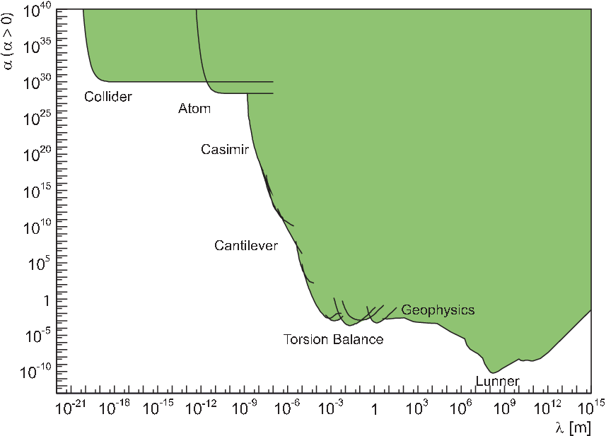
In 1976, Long claimed that he had found evidence for a distance dependence in of the form at a cm scale [Nature260]. Many laboratory Cavendish-type experiments tried to confirm his result; however, all attempts failed to confirm any violation of the Newtonian inverse square law. Then, in 1986, Fischbach claimed that there must be composition dependence in ; this was based on the reanalysis of the classic Etövösh experiment data [Eotvos1922]. This argument is known as the “fifth force,” which can be expressed as
| (8) |
where is a generalized point charge for particles , divided by their masses , which are normalized by the hydrogen mass [PhysRevLett.56.3]. For example, if the additional Yukawa interaction couples to baryon numbers, is obtained for the -th composition using its atomic mass and baryon number (atomic number). The existence of this new composition-dependent gravitational force, i.e., nonzero , would lead to a violation of universality of free fall at short range. Many experiments tried to find evidence of a composition-dependent over various length scales. Although this fifth force proposals essentially introduces a violation of the universality of , experimental constraints on can be set without directly testing for composition dependence using different material combinations; instead, all that is required is merely the test for distance dependence. Therefore, all modern experimental tests on the inverse square law can also test this fifth force proposal. Of course, such tests cannot provide evidence that exists; they can only set upper limits. Following these attempts to find deviations from the Newtonian gravitational inverse square law, since the beginning of 1990’s, we have come to believe that the inverse square law is confirmed to a precision of at cm scale. Very detailed descriptions are summarized in the textbooks written by Fischbach and Talmadge [fischbach1999search] and by Franklin [franklin1993fifth].
Then in 1998, a striking model of large extra-dimensions was proposed by Arkani-Hamed, Dimopoulos, and Dvali (ADD model). This model predicts a violation of the gravitational inverse square law at approximately 0.1 mm, provided that there are two additional “large” spatial dimensions outside our four-dimensional space-time; these extra-dimensions were invoked to naturally resolve the so-called hierarchy problem [Arkani.Hamed1998263, PhysRevD.59.086004]. Figure 2 illustrates the force strength of the four fundamental interactions as functions of distance between two quarks or two electrons. The linear slopes represent the inverse square law . Although Figure 2 is not based on rigorous calculation, we can grasp a rough estimate of the relation between the fundamental interactions. Note that the gravitational inverse square law has been precisely tested only at above laboratory scale, where the line is solid; the region wherein the gravitational force has not been observed is shown as a dashed line. In contrast, the electric force law has only been tested at below laboratory scale. The other two interactions, the strong and weak interactions, tend, by a renormalization calculation, to have the same order of force strength as the electric force at around m. From Figure 2, the hierarchy problem can be visually interpreted as the big gap between gravity and the three other interactions at below collider scales of m, which corresponds to a de Broglie wave length at TeV energies.

In the ADD model, the modified potential
| (9) |
is expected at by assuming a higher dimensional Planck mass of . Here, is a new (4+2)-dimensional gravitational constant. More generally, the ADD potential can be expressed as
| (10) |
using the size of the large extra dimensions . Here, is obtained from a connecting condition at . In this model, the modification of the inverse square law is expected at a scale smaller than , i.e., ; therefore, we can use as in the expressions. (10) can be understood by assuming an isotropic three-dimensional space viewed from a large scale and an isotropic (3+n)-dimensional space at a small scale by Gauss’s law. The expression of these in a single smooth functional form is more convenient,
| (11) |
Obviously, for , (11) cannot be approximated by the Yukawa form in (5). For example, at very short scales, modification factors from the Newtonian potential are ; however, , at . Since all results from experimental tests after Fujii’s proposal have been expressed in the Yukawa parametrization, the latest generation precision experiments at below mm scales, which are searches for a signal of the large extra-dimension, have also tried to constrain the parametrization of (, ) in (5). Therefore, the direct comparisons of the experimental sensitivities of the ADD model using the Yukawa potential between different experiments, which were performed at very different separation distances, are confusing. Instead, in this paper, we propose to use the power-law parametrization in tests of the ADD model. In the following sections, we describe how to compare model sensitivities based on both the Yukawa and power-law parametrizations.
2 General formalism of the experimental tests
Let us first consider how to treat non-Newtonian gravity in a general way. In principle, we cannot perform a direct measurement of the absolute potential . Instead, a differential of the potential, i.e., the force, is usually the quantity to be measured. A modified gravitational force can be written as
| (12) |
where the additional term represents the -dependence of the gravitational constant. Then, a generalized gravitational constant
| (13) |
is obtained. Experimental confirmation of implies a nonconstant . If the distance-varying is experimentally measured as a function of at many distance points, then the functional form of can be determined. At present, in the search for the first evidence of a nonzero , we can test (13) just by comparing at two different measuring distances, and . If we define new experimental parameters
| (14) |
deviation from or implies the violation of the inverse square law. In general, if an experimental result for is obtained, we assume a model for with unknown parameters, and then, evaluate them, for example, in the Yukawa parametrization or in the power-law parametrization.
2.1 Measurement of
Here we consider the methods to experimentally measure . One way is to measure an absolute value of and then compare it with results from other experiments performed at other length scales (absolute measurements). The other way is to perform an experiment that includes measurements at different distances (relative measurements).
2.1.1 Absolute measurements.
The simplest way to determine is to measure the gravitational constant at as and then compare it with results from other experiments, such as at as . Then, we can form
| (15) |
The experimental precision for is limited by that of at around ; therefore, this treatment can be used only at or above approximately 0.1 % precision in . Needless to say, this approach cannot be applied for a length scale at .
To determine an absolute value for , we need to know the absolute values of the measured force, masses, and distances to be used in
| (16) |
To avoid the uncertainties in these experimental parameters, we should try relative measurements where many of the uncertainties cancel one another. Based on the current experimental precision of the plot shown in Figure 1, this absolute measurement may be useful at very short scales below 0.1 mm.
2.1.2 Relative measurements.
A smart way to avoid the uncertainties in absolute measurements is to perform a set of measurements that include at least two different distances in the same experiment. Then, can be obtained directly from
| (17) |
using only the ratios of experimental parameters. Here, are the masses used in the near and far configurations. For example, we can avoid the demanding absolute determinations of the masses. For absolute measurements, if the measurements are performed using torsion balances, cantilevers, or other elastic body devices, their spring constants need to be determined to obtain absolute values for the forces. However, in relative measurements, the spring constants are the same for the near and far settings; therefore, they do not have to be precisely determined to obtain . Such relative measurements are a powerful way to achieve a precise determination below the currently known precision of . Furthermore, for , a relative measurement is the only way to test for the existence of .
2.1.3 Null measurements.
Many relative measurements are, in fact, performed as so-called null experiments. These experiments are designed to keep
| (18) |
under the expectation that for Newtonian gravity. Therefore, any imbalance between and implies . Such null measurements are sometimes useful for improving the precision of force measurements. This is because a measuring dynamic range can be set as small as possible to obtain a large measuring gain (magnification). Application of the null measurement itself does not improve the precision; however, it can reduce the measuring dynamic range, which can help improve the reading resolution. Nevertheless, if the precision is dominated by random mechanical movements, a reduced dynamic range does not improve precision.

In Figure 3, three examples of null configurations are shown using balances. In these experiments, torques from the two different source masses, which are located at different distances from the nearest test mass, are designed to be balanced. If we ignore cross forces between the test and source masses, which are set on opposite ends of a balance bar for simplicity, the null conditions can be written as for (a) and (b), and for (c).
The null condition means that such measurements are “static,” without large dynamic movements due to gravity. Therefore, we can avoid nonlinearity of the spring constant in the measuring device. Such relative measurements can avoid uncertainties in the absolute determination of spring constants; however, experimental determination should be carefully performed by including nonlinearities, i.e., possible deviations from Hooke’s law. Such null measurements can avoid nonlinearity problems in calibration between measured displacements and applied force strengths.
2.2 Model parametrizations
Next, we consider how a measured value of can be interpreted in terms of model parameters. We consider two types of parametrization: the Yukawa parametrization defined in (5) and the power-law parametrization defined in (11). For simplicity, we start the treatment assuming point masses. Then, finite size corrections are discussed.
2.2.1 Yukawa parametrization.
Since the Yukawa potential can represent boson exchange forces, many proposed new physics models can be expressed in this parametrization. See [Adelberger:2009zz] and [Long199923] for the proposed models. The large extra-dimension model can also be parametrized using the Yukawa form for the lowest order diagram wherein . First, we show how experimental constraints can be determined. In (12), is expressed as
| (19) |
therefore,
| (20) |
By solving this equation, we can obtain an expression for as a function of
| (21) |
with . Then, if we can ignore uncertainties on , experimental constraint on can be set as
| (22) |
using the experimental value of , including its error. Then (21) can be re-written as
| (23) |
The numerator can be understood as a rapid falling of at , and the denominator can be understood as a relatively weak rising at in the plot. This function has a minimum at around . Typical examples of (23) are shown in Figure 4.

.
As shown in Figure 4, when , the minimum occurs around . Therefore, the minimum in roughly represents the precision of in the measurement. For absolute measurements using as , the corresponding experimental constraints should be limited to , because is not usually well defined. Therefore, in absolute measurements, there should not be a weak rising in at large . This implies that a single exponential form provides a good approximation for absolute measurements at small measuring distances ,
| (24) |
All experiments at below m scales can be treated in this simple form, provided that the object is small enough to ignore the finite size effect described in Section 2.2.3.
2.2.2 Power-law parametrization.
In addition to the large extra-dimension model, other models also predict non-Newtonian gravity in the power-law form; these are introduced in [doi:10.1142/S0217751X02013356]. For the power-law parametrization, in (12) is expressed as
| (25) |
In general, the exponent does not have to be an integer. In the ADD model, represents the number of large extra-dimensions, which is usually treated as an integer . Just as for the Yukawa parametrization, the corresponding can be expressed as
| (26) |
which can be rewritten as
| (27) |
Typical examples of this function are shown in Figure 5. For comparison, the parameter set in Figure 5 is the same as that used in Figure 4. Here, only attracting cases ( in the Yukawa parametrization) is treated in the power-law parametrization.

As shown in Figure 5, at large , is limited to . Note that the slopes are opposite for large and small . Therefore, for small , a precision measurement with small can set constraint at very small region relative to the experimental scale ; however, a rough measurement with large can set constraint only at very large regions. As we will see in Section 4, this is why, at small , high-energy collider and short-range gravity experiments meet each other at the same 0.1 mm scale , in the context of the large extra-dimension.
2.2.3 Finite size effects.
In real laboratory experiments, all objects have finite sizes. Since we are not assuming the inverse square law, we cannot assume that forces between finite objects are the same as those between point masses, even for spherical objects. The modified potential must be volume integrated over each object; however, can be regarded as almost constant at , if is very small compared with the center-to-center distance or to the surface-to-surface separation (gap) of the objects. Therefore, finite size effects need to be considered for at only above around the experimental scale. This effect is most significant for thick parallel plates with a small separation gap .
Here, two parallel plates with infinite sizes are considered. The force density (for a unit area) between infinite plates with thicknesses and placed at separation gap of can be calculated by
| (28) |
where is mass volume density of the two plates, while and the vertical coordinates penetrating each plate in the outward direction. Then, the distance between small volume elements at and is . Just as for point mass calculations, measurements at two different distances and are required. Then, the force ratio at and can be expressed as
| (29) | |||||
For the Yukawa parametrization, this equation can be solved as
| (30) |
where , and
| (31) | |||||
Finally, can be obtained by
| (32) |
where the volume correction term is defined as
| (33) | |||||
The first exponential factor in (32) represents a rapid falling at . The finite size effect is most significant at the “kink” point at , which is shifted down from the “hinge” point at in the point-mass calculation. These experiments involve very short distance measurements between point masses separated by . Then, a constraint similar to that from point-mass calculation at is yielded. Typical examples are shown in Figure 6. Clear kink positions at can be seen. Here, the and positions are defined as center-to-center distances, as shown in Figure 6.


For the power-law parametrization, we have
| (34) |
where
| (35) |
| (36) |
Typical examples are shown Figure 7. The figure shows the shifting of values at large from to .
Figures 6 and 7 show that finite size effects are significant for the configuration . Contributions from closest volume elements can be regarded as point-mass contributions mixed in the measurement. Any finite size effect can be regarded as a superposition of point-mass calculations. In general, a numerical calculation of the volume integration should be performed to obtain the appropriate constraints on the model parameters for a specific experimental configuration; however, characteristics of the finite size effects can be understood in the present parallel-plate calculations.
3 Experimental constraints
Based on the model parametrization analyses in Section 2, analyzed results from existing experiments can be interpreted as constraints on the parameter space.
3.1 Constraints on the Yukawa parametrization
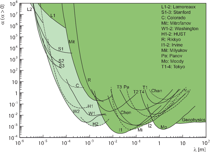
Figure 8 summarizes results from nearly all experimental attempts to test the inverse square law at laboratory scales. Most of the experiments that set constraints at scales were Cavendish-type experiments using torsion balances. These experiments measure gravitational torques from source masses placed near a test mass attached to torsion balance bars. The constraint curves are taken from the original publications and were estimated by the original authors. In Figure 8, all curves correspond to the 95% confidence level.
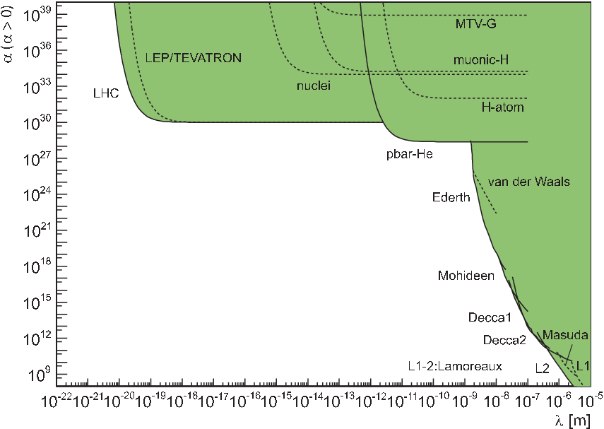
For experiments performed below m scales, results are shown in Figure 9. Experiments in scales used cantilevers as the force sensor instead of torsion balances. Such microscale experiments were performed as gravitational resonance searches at the moving frequency of the source. Experimental sensitivities are far above Newtonian gravity; therefore, the resulting constraints on are very big numbers at .
At distance scales below , experiments measuring the Casimir force were used as the input data to constrain the strong gravity. At this scale, electromagnetic shielding is difficult to place between the source and test masses. Therefore, the dominant forces on the system are the remaining direct electromagnetic forces. Some curves were obtained by independent authors using published experimental data. Especially for the Casimir force measurements, theoretical estimates are themselves complex.
In Figure 9, results from atomic, nuclear, and particle physics data are also plotted. Just as for the Casimir force region, the dominant forces on these systems are known standard model interactions, such as electromagnetic interactions, as well as strong and weak interactions. Therefore, these constraints are estimated to be the maximum allowed strength of strong gravity within the experimental precision of the standard model interactions. Most of these constraints on parameter space (hydrogen atom, antiprotonic (pbar) helium atom, muonic hydrogen, LEP/TEVATRON/LHC) were obtained in the present study, as described in Section 5.3. Note that the results from high-energy collider experiments assume graviton-producing phenomena; in contrast, other nuclear and atomic data were analyzed by assuming classical gravitational phenomena. Therefore, the theoretical reliabilities used in the evaluations are very different.
3.2 Constraints on the power-law parametrization
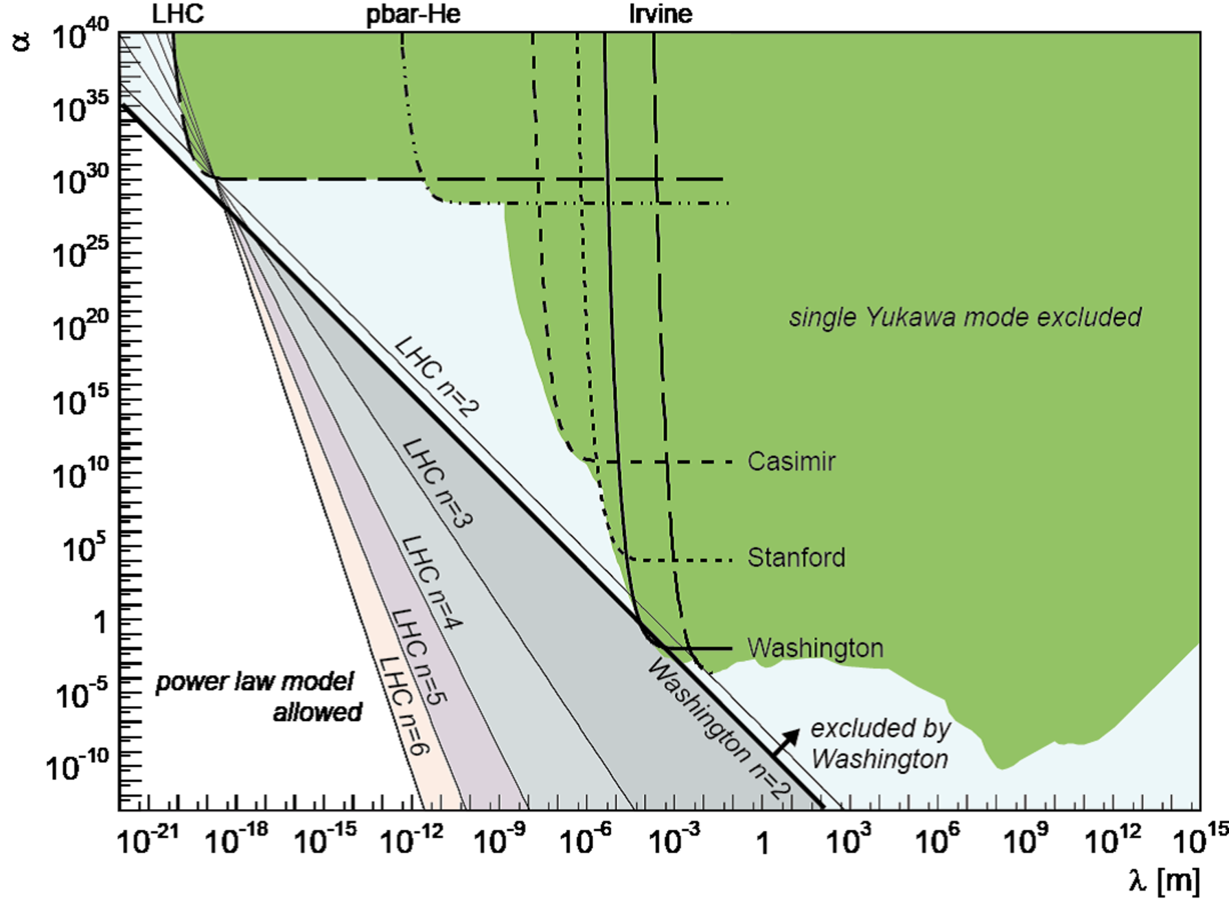
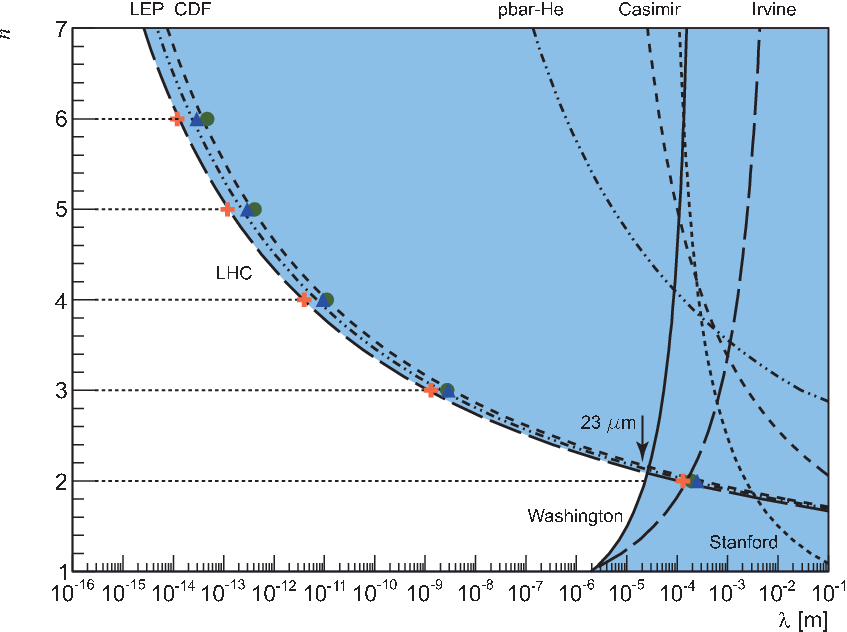
Constraints on the power-law parameter space have not been reported for most experiments, except collider experiments, which did not report results for the Yukawa parametrization. To set experimental constraints on the parameter space in the power-law parametrization without using raw experimental data, such as , several typical constraint curves on the space were chosen, as shown in Figure 10. These representative curves were selected to reproduce the important kink points (for Irvine, Washington, Stanford, Casimir, pbar-He, and LHC), using the point-mass formula in (21). Then, the corresponding values of for these representative curves can be obtained; this enables us to interpret the constraints in the Yukawa form in terms of the power-law form. The results are shown in Figure 11. Results from collider experiments were obtained assuming the ADD model; this allows us to interpret the results obtained as “ vs ” in the form of . The upper limits on were obtained from the Washington data for and from the LHC data for .

4 Discussion on the ADD model
To compare results from the short-range experiments and those from collider experiments, it is useful to express the results in parameter space. The relation between and was obtained assuming the ADD model
| (37) |
where the Planck mass was estimated using Einstein’s gravitational constant instead of Newtonian gravitational constant . Figure 12 shows the resulting plot that corresponds to the plot in Figure 11. Moreover, the experimental lower limits on were determined from the Washington data for and from the LHC data for .
The results from the Washington data at are interpreted as and . This constraint is stronger than that in the original publication by the University of Washington group [PhysRevLett.98.021101] wherein corresponding values were estimated from an plot by searching over at [Ann.Rev.53] and assuming Yukawa potential approximation; the latter is valid if the experiment is performed around . As discussed in Section 1, the ADD model is primarily expressed in a power-law functional form. However, the conventional Yukawa form can only be applied near by assuming that lowest order diagram exchanges the lightest graviton. Indeed, interpretation of in the ADD model in terms of the Yukawa parameter is possible, as has been calculated by some authors [Kehagias200039, Ann.Rev.53]. For a very small experimental distance , must become very large due to the power-law form. However, such magnification at very short distances cannot be represented by constant parameter in the Yukawa parametrization. In fact, should be modified if the Yukawa parametrization is applied to analyze experimental data obtained at . Setting indicates that physical phenomena obey a power-law-type dependence, but for experimental data analyzed using the Yukawa form, a modified can be expressed by
| (38) |
for point-mass calculations. This means that seems to be amplified at a small experimental scale , if the actual gravitational potential obeys the power-law form. To obtain the original strength at , the amplification factor must be removed. The amplification factor is
| (39) |
and a corrected for the simple exponential function in (24) can be obtained
| (40) |
which is not constant but a function of and . The resulting corrected is plotted in Figure 10 for the LHC data in , and for the Washington data at . It is now clear that the experimental sensitivities should be compared with the inclined lines for each . For , the slope is . To compare the sensitivities in the ADD model on the plot, the constraint curves need to be rotated until the corrected lines become horizontal. Then, the Washington kink is the deepest valley in the vertical direction for this line. Figure 10 clearly shows that the tightest constraints are set by the LHC data for and that the scale is the best position to constraint for .
5 List of Experiments
In this section, we briefly introduce the experiments that provided the data used in Figures 8 and 9. All the experiments involved test and source masses; the forces between them were measured. In a laboratory experiment using a torsion balance, the effects of other forces can be reduced by placing an electric shield between the test and source masses, so that the measured force can be regarded as being dominated by gravity. Then, the suppression of Newtonian gravity helps test the inverse square law. In a microscopic measurement, the gravitational force is hidden in the dominant background from Coulomb forces, including the Casimir force. Therefore, only an upper limit on the non-Newtonian strong gravity can be determined. Atomic and sub-atomic systems can be regarded as test systems similar to microscopic measurements wherein standard model backgrounds cannot be avoided.
5.1 Torsion balance experiments
Most experimental tests of the inverse square law have been performed using Cavendish’s torsion balances. These measurements were triggered by Long’s experimental claim for a violation of the inverse square law [Nature260]; this claim was published after his reanalysis of existing data [PhysRevD.9.850], which was indicating a violation of the inverse square law. Subsequently, Soviet groups performed a few important precision measurements at cm scale using classic torsion balance bars: (Figure 13) with at 0.4 m [Sov-JETP50], (Figure 14) with at 6 cm [Sov-JETP61], and (Figure 15) with at 2 mm [Sov-JETP67]. In the 1980s, the University of Irvine group performed a couple of very accurate measurements using static torsion balance bars, which to date still set the tightest constraints at cm scale: (Figure 17) with at 10 cm [PhysRevD.32.3084], (Figure 16) with at 2 cm [PhysRevLett.44.1645]. The Cavendish laboratory group used a torsion balance bar (Figure 18) with at 10 cm [Proc.R.Soc.Lond]. The University of Maryland group performed experiments without using torsion balances but utilizing superconducting gravity gradiometers with at 80 cm [PhysRevLett.49.1745], and with at 1 m [PhysRevLett.70.1195], which still gives the best limit at the 1 m scale. Similarly, Goodkind also performed a superconducting gravimeter experiment with at 1 m [PhysRevD.47.1290]. The University of Tokyo group performed a series of experiments utilizing gravity wave antenna: with at 2 m [Nature283], with at 50 cm [PhysRevD.26.729], (Figure 19) with at 10 cm [PhysRevD.32.342], and (Figure 19) with at 7 mm [PhysRevD.36.2321]. A similar gravity wave antenna experiment was performed at CERN [astone1991]. All these results are consistent with the inverse square law. The most significant result is that from the Irvine group.
The second impact on this field was the proposal of the large extra-dimension model [Arkani.Hamed1998263]. The striking prediction of a possible violation of the inverse square law at around 0.1 mm triggered many recent sophisticated experiments. Before then, the tightest constraint was given by the result of Mitrofanov [Sov-JETP67]. The University of Washington group (Eöt-wash) obtained a very strong constraint at 1 mm using a torsion pendulum with missing mass holes on a test disk [PhysRevLett.86.1418, PhysRevD.70.042004]. They also obtained an upgraded result (Figure 20) with at 0.5 mm [PhysRevLett.98.021101]. Many results from the Eöt-wash group were introduced in [Adelberger:2009zz], not only for the inverse square law but also for other gravity-related measurements.


The group at Huazhong University of Science and Technology (HUST) performed torsion balance experiments (Figure 21) using parallel plates in null configurations [PhysRevLett.98.201101, PhysRevLett.108.081101]. They obtained the best constraint of at 1 mm. The Rikkyo University group also performed torsion balance experiments (Figure 22) using a digital image sensor and obtained a preliminary result of at 5 mm [HE_News.32.2014]. This group is also testing the universality of free fall with a composition-dependent test [1742-6596-453-1-012007].
The University of Colorado group responded to the large extra-dimension model very quickly and obtained a result of at (surface-to-surface separation) using a planar oscillator (Figure 23) as a gravity sensor [Long199923, Nature.01432]. Unlike the HUST and Washington experiments, this experiment did not observe a nonzero gravity signal because of its sensitivity; therefore, only an upper limit on the gravitational force was determined. Similarly, all experiments that followed were performed at below 0.1 mm scales and could not observe a nonzero gravity signal.


Very high-precision experiments were performed (Figure 24) by the Stanford University group using cantilevers [PhysRevD.72.122001, PhysRevD.78.022002, PhysRevLett.90.151101]. They obtained at m (surface-to-surface separation). Most recent experiments testing the large extra-dimension model achieved good precision at the separation gap because of the finite size effects shown in Figure 6.
5.2 Casimir force experiments
In this section, we introduce experiments that provided the data in Figure 9. Unlike torsion balance experiments in which is obtained, the experimental sensitivities in this region are far beyond the strength of Newtonian gravity. Therefore, all constraints were obtained as upper limits on the strength of the gravitational force, which corresponds to the experimental and theoretical precision for the dominant electric force . In the scale below m, it is difficult to place electric shield between the source and test masses. Upper limits on gravity can be estimated by
| (41) |
provided the experimental results are consistent with the electric force calculation. Then,
| (42) |
can be estimated using the ratio of electric force to Newtonian gravity and a relative resolution of the electric force; here, includes both experimental and theoretical errors.
There have been many Casimir force experiments that measure electric forces between two metal surfaces. Because of the difficulty of preparing plates as thin as the measuring separation gap , the data show the curve with kinks at , which are similar to that shown in Figure 6. Although not all experiments were intended to test the gravitational law, their results can be used to set the upper limits on using (42). Lamoreaux at the University of Washington performed Casimir force experiments (Figure 25) with at [PhysRevLett.78.5] and later with at [PhysRevLett.107.171101]. Masuda obtained (Figure 26) at [PhysRevLett.102.171101]. Obrecht et al. also tested in the m range, measuring Casimir-Polder forces [PhysRevLett.98.063201], which were analyzed in [PhysRevD.83.075004]. There are many other analyses by Bordaq and Mostepanenko et al.[PhysRevD.47.2882, PhysRevD.58.075003, PhysRevD.62.011701, PhysRevD.63.115003, doi:10.1142/S0217751X02013356, PhysRevD.81.055003, PhysRevD.83.075004]. Bao et al. also tested below the 200 nm range [PhysRevLett.105.250402]. Decca et. al. at Indiana-Purdue University tested (Figure 27) with at [PhysRevLett.94.240401, PhysRevD.75.077101]. The University of California, Riverside group tested with at [PhysRevA.62.052109]. Ederth in the Sweden Royal Institute of Technology tested (Figure 28) with at [PhysRevA.62.062104], which was analyzed in [PhysRevD.63.115003]. In addition to Casimir force measurements, van der Waals force measurements were performed [Israelachvili21111972], which were analyzed in [Bordag199435]. These data approach at 1 nm. As we saw in Figure 10, these data do not strongly constrain the ADD model at the present precision, compared with the mm scale and collider experiments.


5.3 Atomic, nuclear and particle experiments
Atomic and nuclear systems can also be used to estimate the maximum allowed strength of gravity at microscopic scales using (42), where now represents the known standard model interactions. For atomic systems, these interactions correspond to the Coulomb interaction between nuclei and electron (or other such negatively charged particles for exotic atoms), and for nuclear systems, they correspond to the nuclear force between nucleons inside nuclei. For an example, in an atomic system,
| (43) |
can be obtained for a system in which a particle with mass and charge is orbiting a nuclei with mass and charge .
Figure 9 shows estimated results for hydrogen, the antiprotonic (pbar) helium atom, and the muonic hydrogen atom [INPC2013]. Their relative precisions
| (44) |
can be estimated using relative errors in the experiments (e.g., error of atomic transition frequency) and theories, including physical constants (e.g., Planck constant, fine structure constant, and Rydberg constant). These estimates were performed for the present paper using data from CODATA [RevModPhys.84.1527] for the hydrogen atom, the ASACUSA experiment [PhysRevLett.91.123401, PhysRevLett.96.243401] for the antiprotonic helium atom, and the PSI experiment [Nature466] for the muonic hydrogen atom. The PSI data are not consistent with the known proton radius; nevertheless, the data can be used to set the gravitational upper limit. Details of the calculations will be published separately [Tanaka-future]. Several similar theoretical attempts have been made to constrain strong gravity at this scale for the muonic hydrogen atom [doi:10.1142/S0218271814500059] and for the antiprotonic helium atom [Salumbides201465, Bordag199435]. Nuclear charge radii have also been used as a gravity sensor, in which a modification of the nuclear charge radius is estimated from strong gravity [0954-3899-40-3-035107]. An electron nuclear scattering experiment (the MTV-G experiment); [1742-6596-453-1-012018] was performed to constrain a strong geodetic precession of a scattering electron utilizing a detector setup from the MTV experiment for testing time reversal symmetry [hyperfine]. Of these, the best precision was obtained from the antiprotonic helium spectroscopy data because of the heavy mass of the antiproton. Constraints from a hydrogen system are limited, not by the experimental precision of but by the precision for the Planck constant at .

Similar to the atomic and nuclear tests, particle collision data can also be used to perform similar analyses that constrain the maximum allowed probability (cross section) of gravitational phenomena above standard model predictions. Several graviton-producing channels can be used; however, the simplest is the real graviton emission , and shown in Figure 29. The cross-sectional excess on a monojet produced from the standard model predictions can set upper limits on the gravitational coupling strength. Here, the graviton () cannot be observed, unlike quarks () or gluons (), creating QCD jets in the final states. In this channel, only one visible jet is observed; however, the emitted graviton is not observed, so the event is recognized by observing only one jet with large missing momentum. By comparing with the standard model backgrounds, an upper limit on the monojet production cross section can be estimated. Together with mini-black-hole production, which can be expected in strong gravity, results have already been published for the LEP ( GeV); [arXiv:hep-ex0410004], for the TEVATRON ( TeV); [PhysRevLett.101.181602, PhysRevLett.86.1156], and for the LHC ( TeV); [PhysRevLett.110.011802, Aad2011294, CMS-JHEP]. In collider experiments, is the prime quantity to be determined as a function of ; then, is transformed to using the ADD model (37). All atomic, nuclear, and particle experiments cannot completely shield the standard model contributions (backgrounds); therefore, the resulting precision is poor because is much larger than . However, because of their extreme short measuring distances , they can be sensitive to large values of in power-law type models, as shown in Figure 11, which amplify at a short range.
Among all microscopic experiments, the collider experiments are the only sensitive tool that can compete with the 0.1 mm scale experiments for . For , none of the laboratory-scale experiments can compete with the collider experiments.
6 Summary
We have presented rough estimation procedures based on the Yukawa and power-law parametrizations. Although the parametrization has been widely used because of its historical background, it is not always the best way to compare experimental constraints, especially for the large extra-dimension model. A quantitative treatment based on the power-law parametrization has allowed us, for the first time, to compare results from collider experiments with those from short-range gravity experiments. The comparisons show that at , stronger constraints can be obtained from 0.1 mm scale measurements than from collider experiments.
Acknowledgement
Most of the art works were produced with the help of M. Hatori, S. Saiba, T. Sakuta, and E. Watanabe. Presented results from Rikkyo group were obtained by S. Ozaki, Y. Sakamoto, T. Yoshida, R. Tanuma, and Y. Totsuka for the MTV-G experiment, and by H. Murakami, K. Ninomiya for the short-range experiment. This work was supported by JSPS KAKENHI Grant-in-Aid for Challenging Exploratory Research, Grant Number 24654070. The author would like to thank the editorial board of CQG for giving us the opportunity to write this review article.
References
References
- [2] [] Aad G et al. 2011 Physics Letters B 705(4), 294 – 312.
- [4] [] Aad G et al. 2013 Phys. Rev. Lett. 110, 011802.
- [6] [] Aaltonen T et al. 2008 Phys. Rev. Lett. 101, 181602.
- [8] [] Abbott B et al. 2001 Phys. Rev. Lett. 86, 1156–1161.
- [10] [] Adelberger E G, Heckel B R & Nelson A E 2003 Ann. Rev. Nucl. Part. Sci. 53, 77 – 121.
- [12] [] Adelberger E, Gundlach J, Heckel B, Hoedl S & Schlamminger S 2009 Prog.Part.Nucl.Phys. 62, 102–134.
- [14] [] Arkani-Hamed N, Dimopoulos S & Dvali G 1998 Physics Letters B 429(3–4), 263 – 272.
- [16] [] Arkani-Hamed N, Dimopoulos S & Dvali G 1999 Phys. Rev. D 59, 086004.
- [18] [] Ask S 2004 arXiv:hep-ex p. 0410004.
- [20] [] Astone P et al. 1991 Zeitschrift für Physik C Particles and Fields 50(1), 21–29.
- [22] [] Bao Y, Guérout R, Lussange J, Lambrecht A, Cirelli R A, Klemens F, Mansfield W M, Pai C S & Chan H B 2010 Phys. Rev. Lett. 105, 250402.
- [24] [] Bezerra V B, Klimchitskaya G L, Mostepanenko V M & Romero C 2010 Phys. Rev. D 81, 055003.
- [26] [] Bezerra V B, Klimchitskaya G L, Mostepanenko V M & Romero C 2011 Phys. Rev. D 83, 075004.
- [28] [] Bordag M, Geyer B, Klimchitskaya G L & Mostepanenko V M 1998 Phys. Rev. D 58, 075003.
- [30] [] Bordag M, Geyer B, Klimchitskaya G L & Mostepanenko V M 2000 Phys. Rev. D 62, 011701.
- [32] [] Bordag M, Mostepanenko V & Sokolov I 1994 Physics Letters A 187(1), 35 – 39.
- [34] [] Chan H A, Moody M V & Paik H J 1982 Phys. Rev. Lett. 49, 1745–1748.
- [36] [] Chatrchyan S et al. 2012 Journal of High Energy Physics 2012(9).
- [38] [] Chen Y T, Cook A H, F.R.S. & Metherell A J F 1984 Proc. R. Soc. Lond. A 394, 47 – 68.
- [40] [] Chiaverini J, Smullin S J, Geraci A A, Weld D M & Kapitulnik A 2003 Phys. Rev. Lett. 90, 151101.
- [42] [] Decca R S, López D, Chan H B, Fischbach E, Krause D E & Jamell C R 2005 Phys. Rev. Lett. 94, 240401.
- [44] [] Decca R S, López D, Fischbach E, Klimchitskaya G L, Krause D E & Mostepanenko V M 2007 Phys. Rev. D 75, 077101.
- [46] [] Ederth T 2000 Phys. Rev. A 62, 062104.
- [48] [] Eötvös R v, Pekár D & Fekete E 1922 Ann. Phys. (Leipzig) 68, 11–66.
- [50] [] Fischbach E, Sudarsky D, Szafer A, Talmadge C & Aronson S H 1986 Phys. Rev. Lett. 56, 3–6.
- [52] [] Fischbach E & Talmadge C 1999 The search for non-Newtonian gravity Springer Verlag.
- [54] [] Franklin A 1993 The Rise and Fall of the Fifth Force American Institute of Physics.
- [56] [] Fujii Y 1971 Nature Physical Science 234, 5–7.
- [58] [] Fulcher L P 1986 Phys. Rev. A 33, 759–761.
- [60] [] Geraci A A, Smullin S J, Weld D M, Chiaverini J & Kapitulnik A 2008 Phys. Rev. D 78, 022002.
- [62] [] Goodkind J M, Czipott P V, Mills A P, Murakami M, Platzman P M, Young C W & Zuckerman D M 1993 Phys. Rev. D 47, 1290–1297.
- [64] [] Harris B W, Chen F & Mohideen U 2000 Phys. Rev. A 62, 052109.
- [66] [] Hirakawa H, Tsubono K & Oide K 1980 Nature 283, 184–185.
- [68] [] Hori M, Dax A, Eades J, Gomikawa K, Hayano R S, Ono N, Pirkl W, Widmann E, Torii H A, Juhász B, Barna D & Horváth D 2006 Phys. Rev. Lett. 96, 243401.
- [70] [] Hori M, Eades J, Hayano R S, Ishikawa T, Pirkl W, Widmann E, Yamaguchi H, Torii H A, Juhász B, Horváth D & Yamazaki T 2003 Phys. Rev. Lett. 91, 123401.
- [72] [] Hoskins J K, Newman R D, Spero R & Schultz J 1985 Phys. Rev. D 32, 3084–3095.
- [74] [] Hoyle C D, Kapner D J, Heckel B R, Adelberger E G, Gundlach J H, Schmidt U & Swanson H E 2004 Phys. Rev. D 70, 042004.
- [76] [] Hoyle C D, Schmidt U, Heckel B R, Adelberger E G, Gundlach J H, Kapner D J & Swanson H E 2001 Phys. Rev. Lett. 86, 1418–1421.
- [78] [] Israelachvili J N & Tabor D 1972 Proceedings of the Royal Society of London. A. Mathematical and Physical Sciences 331(1584), 19–38.
- [80] [] Kapner D J, Cook T S, Adelberger E G, Gundlach J H, Heckel B R, Hoyle C D & Swanson H E 2007 Phys. Rev. Lett. 98, 021101.
- [82] [] Kehagias A & Sfetsos K 2000 Physics Letters B 472(1–2), 39 – 44.
- [84] [] Kuroda K & Hirakawa H 1985 Phys. Rev. D 32, 342–346.
- [86] [] Lamoreaux S K 1997 Phys. Rev. Lett. 78, 5–8.
- [88] [] Long D R 1974 Phys. Rev. D 9, 850–852.
- [90] [] Long D R 1976 Nature 260, 417–418.
- [92] [] Long J C, Chan H W, Churnside A B, Gulbis E A, Varney M C M & Price J C 2003 Nature 421, 922 – 925.
- [94] [] Long J, Chan H & Price J 1999 Nuclear Physics B 539(1–2), 23 – 34.
- [96] [] Masuda M & Sasaki M 2009 Phys. Rev. Lett. 102, 171101.
- [98] [] Milyukov V K 1985 Sov. Phys. JETP 61, 187 –191.
- [100] [] Mio N, Tsubono K & Hirakawa H 1987 Phys. Rev. D 36, 2321–2326.
- [102] [] Mitrofanov V P & Ponomareva O I 1988 Sov. Phys. JETP 67, 1963 –1966.
- [104] [] Mohr P J, Taylor B N & Newell D B 2012 Rev. Mod. Phys. 84, 1527–1605.
- [106] [] Moody M V & Paik H J 1993 Phys. Rev. Lett. 70, 1195–1198.
- [108] [] Mostepanenko V M 2002 International Journal of Modern Physics A 17(29), 4307–4316.
- [110] [] Mostepanenko V M & Novello M 2001 Phys. Rev. D 63, 115003.
- [112] [] Mostepanenko V M & Sokolov I Y 1993 Phys. Rev. D 47, 2882–2891.
- [114]
[]
Murata J, Tanaka S, Ninomiya K & Murakami H 2014 High Energy
News (in Japanese) 32, 233–240.
*#1 - [116] [] Murata J et al. 2014 Hyperfine Interaction 255, 193–196.
- [118] [] Newton I 1687 Philosophiæ Naturalis Principia Mathematica.
- [120] [] Ninomiya K, Kishi R, Murakami H, Nishio H, Ogawa N, Taketani A & Murata J 2013 Journal of Physics: Conference Series 453(1), 012007.
- [122] [] Obrecht J M, Wild R J, Antezza M, Pitaevskii L P, Stringari S & Cornell E A 2007 Phys. Rev. Lett. 98, 063201.
- [124] [] Ogawa Y, Tsubono K & Hirakawa H 1982 Phys. Rev. D 26, 729–734.
- [126] [] Onofrio R 2014 International Journal of Modern Physics D 23(01), 1450005.
- [128] [] Panov V I & Frontov V N 1979 Sov. Phys. JETP 50, 852 –856.
- [130] [] Pohl R et al. 2010 Nature 466, 213 – 216.
- [132] [] Salumbides E, Ubachs W & Korobov V 2014 Journal of Molecular Spectroscopy 300(0), 65 – 69.
- [134] [] Smullin S J, Geraci A A, Weld D M, Chiaverini J, Holmes S & Kapitulnik A 2005 Phys. Rev. D 72, 122001.
- [136] [] Spero R, Hoskins J K, Newman R, Pellam J & Schultz J 1980 Phys. Rev. Lett. 44, 1645–1648.
- [138] [] Sushkov A O, Kim W J, Dalvit D A R & Lamoreaux S K 2011 Phys. Rev. Lett. 107, 171101.
- [140] [] Talmadge C, Berthias J P, Hellings R W & Standish E M 1988 Phys. Rev. Lett. 61, 1159–1162.
- [142] [] Tanaka S & Murata J (to be published).
- [144] [] Tanaka S, Nakaya Y, Ninomiya K, Nishio H, Onishi J, Openshaw R, Pearson M, Totsuka Y & Murata J 2013 Journal of Physics: Conference Series 453(1), 012018.
- [146] [] Tanaka, Saki, Nakaya, Yusuke, Narikawa, Reiya, Ninomiya, Kazufumi, Onishi, Junichi, Pearson, Matthew, Openshaw, Robert, Saiba, Shuntaro, Tanuma, Ryosuke, Totsuka, Yumi & Murata, Jiro 2014 EPJ Web of Conferences 66, 05021.
- [148] [] Tu L C, Guan S G, Luo J, Shao C G & Liu L X 2007 Phys. Rev. Lett. 98, 201101.
- [150] [] Williams E R, Faller J E & Hill H A 1971 Phys. Rev. Lett. 26, 721–724.
- [152] [] Xu J, Li B A, Chen L W & Zheng H 2013 Journal of Physics G: Nuclear and Particle Physics 40(3), 035107.
- [154] [] Yang S Q, Zhan B F, Wang Q L, Shao C G, Tu L C, Tan W H & Luo J 2012 Phys. Rev. Lett. 108, 081101.