Global Structure of Curves from Generalized Unitarity Cut of Three-loop Diagrams
Abstract
This paper studies the global structure of algebraic curves defined by generalized unitarity cut of four-dimensional three-loop diagrams with eleven propagators. The global structure is a topological invariant that is characterized by the geometric genus of the algebraic curve. We use the Riemann-Hurwitz formula to compute the geometric genus of algebraic curves with the help of techniques involving convex hull polytopes and numerical algebraic geometry. Some interesting properties of genus for arbitrary loop orders are also explored where computing the genus serves as an initial step for integral or integrand reduction of three-loop amplitudes via an algebraic geometric approach.
Keywords
Algebraic Geometry, Loop Amplitude, Unitarity Cut1 Introduction
Algebraic geometry has been introduced to the multi-loop amplitude computation in recent years, responding to the demand of Next-to-Leading-Order or Next-Next-to-Leading-order precision correction for collider experiments. Many attempts have been taken towards the purpose of implementing a systematic and automatic algorithm for two-loop and three-loop amplitude computations, in the language of complex algebraic geometry.
The basic idea of this approach is to generalize traditional concepts, such as integral reduction [1, 2, 3, 4, 5] and unitarity cut [6, 7, 8, 9], from one-loop to multi-loop amplitudes. It is well-known that unitarity can be applied to the computation of one-loop amplitudes from tree amplitudes [10, 11, 12], while it is possible now to compute the tree amplitudes very efficiently via the Britto-Cachazo-Feng-Witten recursion relation [13, 14]. Moreover, one-loop integrals can be algebraically reduced to a linear combination of scalar integrals in the integral basis. The integral basis is a set of a finite number of integrals. For one-loop amplitudes, it only contains scalar box, triangle, bubble integrals in four-dimension, additional scalar pentagon integral in -dimension, and tadpole integral for massive internal momenta. A scalar integral is an integral whose numerator of integrand is one. All one-loop integrals with a tensor structure in the numerator can be reduced by, e.g., Passarino-Veltman reduction [2, 3], to scalar integral basis. Starting from a general integral for a Feynman diagram, we can perform the reduction procedure and keep track of all kinematic factors in each step. Then the coefficients of integral basis can be obtained as a consequence of reduction procedure. However, there is a simpler way of computing the coefficients from tree amplitudes, by matching the discontinuity of integrals under unitarity cuts [15, 16, 17] or generalized unitarity cuts [18, 19]. Assuming that the integral basis is already known, which is indeed the case for one-loop amplitudes, we can formally expand an one-loop integral as a linear combination of integrals in the basis with unknown coefficients. The box, triangle, bubble integrals under unitarity cuts apparently have different signatures, which can be used to identify the kinematic factors of signatures as coefficients of integral basis correspondingly. In the integrand level, the coefficients can also be extracted by reduction methods algebraically [20], with the help of quadruple, triple and double unitarity cuts. This has been extensively suited with numerical implementations [21, 22, 23, 24, 25, 26].
The difficulty of generalizing the one-loop algorithm to multi-loop amplitudes is obvious. First of all, the integral basis is generally unknown. It is known that the integral basis contains not only scalar integrals, but also tensor structure of loop momentum in the numerator. Even for some simple diagrams such as a four-point two-loop double-box diagram where the integral basis is already known [27], unitarity cut method is not directly applicable for determining the coefficients of the integral basis. Algebraic geometric techniques are introduced to overcome these difficulties, and they provide a new interpretation of unitarity cut for multi-loop amplitudes. It is applied both to integrand reduction and integral reduction.
For multi-loop amplitude computations in the language of algebraic geometry, the concept of maximal unitarity cut is replaced by the simultaneous solution of on-shell equations of propagators, instead of delta function constraints. The on-shell equations form the basis of an ideal, and the simultaneous solution set defines the variety of the ideal. In the integrand level [28, 29], the Gröbner basis of the ideal is used as divisors, and polynomial division over these divisors provides a finite set of algebraically independent monomials, which defines the integrand basis of a given diagram, in principle, to any loop orders. The primary decomposition method is applied to study the irreducible components of the ideal and the variety, which is useful for determining coefficients of integrand basis through branch-by-branch polynomial fitting method. These algebraic geometry techniques have already been applied to the study of integrand basis and structure of varieties of all four-dimensional two-loop diagrams, and for explicitly computing some two-loop amplitudes and three-loop amplitudes [30, 31, 32, 33, 34, 35, 36, 37, 38].
In the integral level, the Integration-by-Parts(IBP) method [39, 40, 41, 42] is a traditional way of determining the integral basis from the integrand basis. Recently, an attempt of determining integral basis by unitarity cut method and spinor integration technique has also been presented [43]. Determining the integral basis of multi-loop amplitudes is a non-trivial problem, and one of the bottlenecks is that the computation is time-consuming even with a computer. Thus it deserves more studies at both theoretical [44, 45] and computational levels. Once the integral basis is determined for a given diagram, algebraic geometry can be applied to the computation of their expansion coefficients [46]. Again, this is realized by considering a simple fact that integration of a delta function in is equivalent to a contour integration in by Cauchy’s integral theorem. The latter is in fact the computation of residues at poles surrounded by chosen contours. In order for it to be applied to multi-loop amplitude computations, it should be generalized to multivariate analytic functions, which leads to the computation of multivariate residues at global poles. The global poles are determined by the simultaneous solution of on-shell equations of propagators, and it requires the study of ideal and variety of on-shell equations. The coefficients of integral basis are computed as a linear combination of contour integrations at some chosen global poles determined by the global structure of variety. This method has already been applied extensively to four-dimensional two-loop double-box integral and crossed-box integral, and to the study of three-loop integrals and also integrals with doubled propagators [47, 48, 49, 50, 51, 52, 53, 54].
In both multi-loop integral reduction and integrand reduction through an algebraic geometric approach, we can see that the equivalent description of maximal unitarity cut, i.e., the simultaneous solution (variety) of on-shell equations of propagators (ideal), plays fundamental role. Although, in principle, such an algebraic geometric approach can be applied to any loops, the explicit application is still limited to a few two-loop and three-loop diagrams due to the complexity of computation. Thus, before a wider application to other two-loop and three-loop diagrams, it would be better as an initial step to study the global structure of varieties for all two-loop and three-loop diagrams.
A four-dimensional -loop amplitude has degrees of freedom, and it defines an integral in complex plane in the algebraic geometry framework. By Hilbert’s Nullstellensatz, the number of propagators can be reduced to . The polynomials of propagators for a given diagram define an ideal in the polynomial ring . If , the ideal is zero-dimensional, and the corresponding variety is a finite set of points in . If , the ideal is one-dimensional, and the corresponding variety is an algebraic curve. This curve may be reducible, and could consist of several irreducible curves. However, the algebraic curve can be universally characterized by its geometric genus, which is a topological invariant. For a specific diagram with propagators, if the algebraic curve defined by the variety has genus , then the global structure of variety is described by a -fold torus or its degenerate pictures. If , the ideal is higher-dimensional and the corresponding higher-dimensional variety is more complicated to study.
In [55], the arithmetic genus and singular points of an algebraic curve are introduced to study the geometric genus of curves defined by one-loop, two-loop and some of three-loop diagrams. In this paper, we generalize the study of global structure to all four-dimensional three-loop diagrams with eleven propagators. The Riemann-Hurwitz formula is applied to the study of genus, and an algorithm based on numerical algebraic geometry [56, 57] is implemented to compute necessary terms in the Riemann-Hurwitz formula. With this algorithm, it is possible to study the global structure of curves defined by four-loop diagrams efficiently. For some three-loop diagrams, a recursive formula derived from the Riemann-Hurwitz formula is presented to study the genus of three-loop diagrams recursively from the genus of two-loop diagrams, where a lattice convex polytope method is adopted. As of theoretical interests, some interesting phenomena regarding the genus of any loop orders are explored. We hope that these results could be useful for the integral and integrand reduction of three-loop amplitudes via algebraic geometry in the near future.
The remainder of this paper is organized as follows. In Section 2, we introduce the Riemann-Hurwitz formula for the computation of geometric genus. An algorithm based on numerical algebraic geometry is also discussed for numerically computing the genus of any algebraic curve. In Section 3, we re-study the global structure of curves of two-loop diagrams by the Riemann-Hurwitz formula, and in Section 4, we generalize the analysis to curves of certain three-loop diagrams whose sub-two-loop diagram is double-box or crossed-box. A recursive formula derived from the Riemann-Hurwitz formula is presented for recursively computing genus of curve defined by three-loop diagrams from genus of curve defined by two-loop diagrams. A proof of the recursive formula is provided based on convex polytope techniques. In Section 5, the genus of curves defined by the remaining three-loop diagrams is analyzed by the algorithm. The genus of curves defined by an infinite series of White-house diagrams to any loop orders is also studied as an example of recursive formula for higher loop diagrams. In Section 6, we summarize the results and discuss generalizations for future work.
2 Preliminary
2.1 The Riemann-Hurwitz formula and geometric genus
The Riemann-Hurwitz formula describes the relation of the Euler characteristic between two surfaces when one is a ramified covering of the other. It is often applied to the theory of Riemann surfaces and algebraic curves for finding the genus of a complicated Riemann surface that maps to a simpler surface (for more mathematical details, definition of geometric genus, properties of algebraic curve and other relevant definitions see, e.g., the books [58, 59]).
The Euler characteristic is a topological invariant. For an orientable surface, it is given by , where is the genus. A covering map is a continuous function from a topological space to another topological space
such that each point in has an open neighborhood evenly covered by . In the case of an unramified covering map which is surjective and of degree , we have formula
| (1) |
The ramification, roughly speaking, is the case when sheets come together. The covering map is said to be ramified at point in if there exist analytic coordinates near and such that takes the form , . The number is the ramification index at point . The ramification of covering map at some points introduces a correction to the above formula as
| (2) |
known as the Riemann-Hurwitz formula. Applying this formula to the case of algebraic curves, for a curve of genus and another curve of genus , there is a (ramified) covering map
and the genus of two curves are related by
| (3) |
Note that ramification can also happen at infinity. Knowing the degree of covering map, the genus of curve and the ramification points, it is possible to compute the genus of curve .
A special version of (3) is that the covering map maps a curve to a curve of genus zero. In this case, , and the Riemann-Hurwitz formula (3) is rewritten as
| (4) |
where .
We can either use formula (3) or formula (4) for the genus analysis. For an algebraic curve defined by several polynomial equations, simplifications can be made when a subset of polynomial equations contain fewer variables which also define a curve . In this case, we can compute the degree of the covering map and the ramification points. The computation is relatively simpler than the case of mapping to a curve of genus zero, especially for the curves defined by the maximal unitarity cut of multi-loop diagrams, where analytic study is possible. However, it is always possible to compute the genus of any algebraic systems of curves by formula (4), although the computation would become very complicated. In the next subsection, we will describe an algorithm for computing the geometric genus by formula (4), based on numerical algebraic geometry.
2.2 An algorithm for computing the geometric genus
The algorithm for numerically computing the geometric genus of a curve presented in [60] (see also (61, § 2.6) and (56, § 15.1,§ 16.5.2)) follows from the Riemann-Hurwitz formula using numerical algebraic geometry techniques to compute the necessary items in the formula. The following provides a short description of the techniques needed to describe this algorithm, namely witness sets, computing a superset of the branchpoints, and monodromy, with the books [56, 62] providing more details.
The input for the algorithm of [60] to compute the geometric genus of an irreducible curve is a witness set for . Let be a system of polynomials in variables such that is an irreducible component of the set . A witness set for is the triple where is a general linear polynomial and . The set is called a witness point set for with . The concept of witness sets was described in particle and string theory frameworks in [63, 57, 64].
By, for example, isosingular deflation [65], we can assume that has multiplicity with respect to .
Given a system , we are interested in computing a witness set for each curve that is an irreducible component . To accomplish this, we first select a general linear polynomial and compute the set of isolated points in , which is the union of the witness points sets for each such curve. For example, one could use regeneration [66, 67] and the local dimension test [68] to yield such a set.
The set is partitioned into the various , for example, using many random monodromy loops with the decomposition confirmed using the trace test [69]. Since performing a monodromy loop is a key aspect of computing the geometric genus, we will summarize the computation here for curves. Let define a loop of general hyperplanes in with . Thus, defines a collection of smooth paths with . Since the points and must lie on the same irreducible component, this monodromy loop provides information about how to partition when .
Suppose that is a witness set for an irreducible curve . Let be a general linear projection defined by for . As shown in [60], a finite superset of the branchpoints of with respect to is sufficient since the contribution in the Riemann-Hurwitz formula from points which are not branchpoints is zero. In particular, such a superset is the finite set of points such that
is rank deficient, where is the Jacobian matrix of the system . The set can be computed from a witness set for using regeneration extension [70] with [71].
For each distinct number in , we need to compute the contribution for each in the Riemann-Hurwitz formula. A monodromy loop surrounding that does not include any other point in yields a decomposition of the points into sets with . One also needs to perform a monodromy loop which surrounds every point in to compute the contribution at . Thus, the geometric genus of is
Remark 1
If one performs the algorithm described above for an input witness set of a curve which is not irreducible, then the output is
where are the irreducible components of . This value could be negative.11 1 We thank Andrew Sommese for communicating this remark to us.
2.3 Curves of three-loop diagrams
In this subsection, we classify all the three-loop diagrams whose maximal unitarity cuts yield an algebraic system that defines a non-trivial curve. Naively, there are a large number of three-loop diagrams in four-dimension, with the total number of propagators up to twelve. Diagrams with more than twelve propagators are over-determined, i.e., the number of propagators is larger than the independent parametrization variables of loop momenta. Thus, they can be reduced to diagrams with twelve propagators or lower. Similarly, the number of propagators containing only two of the loop momenta or should be smaller than eight, and the number of propagators containing only one loop momentum or should be smaller than four. If there are no shared propagators between any two loops, i.e., different loops only be connected at vertices, then the integral of three-loop diagrams can be rewritten as product of an one-loop integral and a two-loop integral, or product of three one-loop integrals. So, the topology defined by these diagrams is the same as the one defined by two-loop diagrams or one-loop diagrams. We are only interested in the non-trivial three-loop diagrams with loops being connected by shared propagators.
Basically, there are two types of non-trivial three-loop diagrams as shown in Figure (1). Type I diagram is the ladder type diagram, where loops , have shared propagators, while do not have shared propagators. Type II diagram is the Mercedes-logo type diagram, where any two loops have shared propagators. These diagrams could be planar or non-planar diagrams, according to the value of , where is the number of propagators along the dashed lines in Figure (1). In the current paper, we are interested in the topologies whose maximal unitarity cuts define a curve. So we require the number of propagators to be .
For type I diagram, we take the convention that the left loop is , the middle loop is and the right loop is . Then we have the following inequalities for ,
Of course we have assumed every except , in order to generate all ladder type diagrams. However, due to the symmetries of diagrams, there will be over-counting from the solution of above inequalities. In order to remove the over-counting, we further require that
| (5) |
These inequalities remove the over-counting from symmetries inside each left loop, middle loop and right loop. However, there is still symmetry between the left and right loops. The over-counting of this symmetry can be removed by following two sets of inequalities
| (6) |
The above inequalities generate 36 diagrams, denoted by as
However, if any , then the corresponding loop momentum can be completed determined by the equations of unitarity cuts. So this loop momentum is effectively the external momentum for the remaining loops. In this case, the curve associated with three-loop diagram is reduced to the curve associated with two-loop diagram. Similarly, if any , then the corresponding loop momenta can be completely determined. The curve is reduced to the one associated with one-loop diagram. Among the 36 diagrams, there are still 13 diagrams whose curves can not be reduced to the ones associated with one-loop or two-loop diagrams. We shall study the topologies of these diagrams in the following sections.

For type II diagram, we take the convention that the left-top loop is , the right-top loop is and the bottom loop is . Again we have
Also we have . This type of diagrams has symmetries by exchanging , or or . By considering these symmetries, we can generate 15 diagrams, denoted by as
For diagrams with or , the curves are reduced to the ones associated with one-loop triangle, two-loop double-box or crossed-box diagrams. Among the 15 diagrams, there are eight diagrams which can not be reduced. These are the eight three-loop Mercedes-logo diagrams which we will study in the following sections.
In summary, there are in total three-loop diagrams generating algebraic systems defining non-trivial curves. Among them, 16 diagrams have a sub-two-loop diagram whose maximal unitarity cuts also define curves. For these diagrams, we will present a recursive formula based on Riemann-Hurwitz formula, to compute the genus recursively from two-loop diagrams. The remaining five diagrams can not be computed by the recursive formula, so we will use the algorithm based on numerical algebraic geometry to study the genus.
3 Counting the ramified points of two-loop diagrams
As a warm-up exercise for three-loop analysis, let us briefly go through the study of two-loop diagrams in the framework of Riemann-Hurwitz formula (3). There are two diagrams whose equations of maximal unitarity cuts define non-trivial irreducible curves. As it is well studied in the literature [46, 48, 31, 50], the curve associated with the double-box diagram has genus one and the curve associated with the crossed-box diagram has genus three, obtained by directly computing the arithmetic genus and singular points of the curves, or inferred from the picture of Riemann spheres in the limit of degenerate kinematics.
Notice that these two diagrams can be constructed from a box diagram and a triangle diagram as shown in Figure (2), by opening the vertex in the triangle diagram marked as red circle and connecting the two legs to the box diagram at the vertices marked as black dots respectively. If ignoring all equations from the box diagram, the equation system associated with a triangle diagram itself defines a curve. Referring to the Riemann-Hurwitz formula, the genus of the curve associated with the double-box diagram or crossed-box diagram is related to the genus of curve associated with triangle diagram, by considering the covering map
| (7) |
The cut equations of triangle diagram are given by
The latter two equations are linear in , so there is only one quadratic equation after some algebraic manipulation of above three equations. By solving two variables with two linear equations, the remaining quadratic equation becomes equation of conics, and it is topological equivalent to genus zero Riemann sphere. So, the only lacking data for computing the genus of double-box or crossed-box diagram is the ramified points of covering map (7). Since these two-loop diagrams have been separated into two parts and , for any given point in the curve , the four equations of define points in or . This means that the covering map (7) maps
from curves of two-loop diagrams to curve of triangle diagram. If all are the same point, then the map is ramified at the point , and the ramification index is .
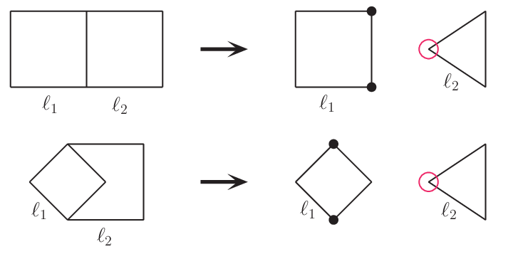
We need to compute the ramified points and their ramification indices in the covering map (7). We use the same parametrization of loop momenta as in [31], and define and as the parametrization variables of and respectively. A function with argument denotes a function whose highest degree monomials are terms of , where could be any elements in . So is a quadratic function of , while is also a quadratic function of , but a linear function with respect to or individually. Among the seven equations of maximal unitarity cuts, there are four linear equations and three quadratic equations. Using the linear equations, we can always solve two of ’s and two of ’s. Define the remaining variables as , then the remaining three quadratic equations are equations of and . The covering map (7) actually maps
Solving the linear equations in double-box or crossed-box diagram, we get
So we can simplify the covering map as
Since is quadratic in but is linear in , they define two covering sheets over Riemann sphere , so the covering map is a double cover. For any given point in the curve , the joint equations can be used to solve , and it has two solutions because of its quadratic property. Generally the two solutions are distinct, however when the discriminant equals to zero, they coincide in the same point and produce a ramified point with ramification index .
Let us generically consider two equations
The discriminant is
| (34) | |||||
A given point in curve should also follow the constraint , if it is a ramified point. So these two equations completely determine the location of ramified points. In the double-box case, all ’s are independent of , while ’s are linear functions of , so the discriminant is a generic quadratic function of . By Bézout’s theorem, the two equations define distinct points, which are the ramified points with index . In the crossed-box case, are independent of , are linear in and are quadratic in , so is a generic function of degree four in . These two equations define ramified points with ramification index . Using Riemann-Hurwitz formula, we get
which agree with the known results in the literature [46, 48, 31, 50].
To summarize, in order to compute the genus of curve associated with two-loop diagrams from genus of curve associated with one-loop diagram, we separate the equations of maximal unitarity cuts into and . For given point in , equations of always give two distinct solutions unless the discriminant of is zero. This additional constraint together with curve equations provide all information about the ramified points.
4 Counting the ramified points of three-loop diagrams
The same discussion can be generalized to compute the genus of curves associated with three-loop diagrams from genus of curves associated with two-loop diagrams, if the three-loop diagram has a sub-two-loop which also defines a curve. For these three-loop diagrams, we can always separate cut equations into together with or . Since and are known, the only data we need to know is the ramified points. For ladder type diagrams, among the eleven cut equations, there are five quadratic equations and six linear equations, while for Mercedes-logo type diagrams, there are six quadratic equations and five linear equations.
We will discuss how to count the ramified points for these two types of diagrams in this section. Defining , and as parametrization variables for respectively, where is the loop momentum in box diagram, the number of ramified points is given by
| (35) | |||||
where , and the ramification indices are . , , , , , are the number of equations containing , , , , , respectively, and , , , , , are the number of linear equations containing , , , , , respectively. Also
where is the floor function giving the integer part of .
4.1 Ladder type diagrams
The ladder type diagrams can be constructed from inserting box diagram into two-loop diagrams at the vertices marked as red circles as shown in Figure (3). Depending on the way of opening the vertices, there are in total seven different ways connecting to the two-loop diagrams, marked as black dots in the seven diagrams in Figure (3).

For this type diagrams, we take the convention that have shared propagators, thus . Then the formula (35) is simplified to
| (36) |
Since can either be one or zero, from (36) we see that could be and . It is also interesting to notice that picks up no information in the loop. In fact, since if and if , we can artificially write . Then (36) can be expressed as
| (37) |
This reformulation provides a diagrammatic meaning for the counting of ramified points which we will show below.
For the ladder type diagrams, the covering map from curves associated with three-loop diagrams to curves associated with two-loop diagrams is given by
Although is a quadratic equation, it is linear in , so there is only one quadratic equation in . Anyway, equations define two covering sheets over Riemann surface or , just as in the analysis of mapping two-loop diagrams to one-loop diagrams. So it is a double cover. Points in the curve defined by , become ramified points if they follow the additional constraint , which is the discriminant (34) of .
Equations , define a zero-dimensional ideal in polynomial ring , and the number of distinct solutions equals to the degree of ideal. The up-bound of distinct point solutions is . Numerically, the degree of ideal can be computed by the Gröbner basis of ideal, which is the degree of leading term in Gröbner basis, by many algorithms (e.g., using Macaulay2 [72]). However, we want to compute the ramified points without explicit computations. Notice that among the seven cut equations of sub-two-loop part, only the four linear equations are different. The linear equations of seven diagrams in Figure (3) are given by
and
It is clear that for , and for , . We can assign a factor
| (87) |
in Figure (3). For the box diagram part, we have for and for . So we can assign a factor
| (88) |
The genus of curves associated with these three-loop ladder type diagrams can be computed from genus of curves associated with two-loop double-box or crossed-box diagram via Riemann-Hurwitz formula as
| (89) |
or diagrammatically as
| (90) |
The computation can be done by just looking at the diagrams.
To finish this subsection, let us present the results for ladder type diagrams. There are 13 diagrams whose cut equations define non-trivial curves. Twelve of them have a sub-two-loop double-box or crossed-box diagram, denoted by as
Genus of these twelve diagrams can be computed by the recursive formula (89) or (90). The construction of these diagrams are shown in Figure (4).

With the known results and , using formula (89), we can compute the genus as
| 5 | 9 | 5 | 9 | 13 | 9 | 13 | |
| 9 | 17 | 9 | 13 | 21 | 13 | 21 |
Note that diagram and are the same diagram, while diagram and are also the same diagram.
4.2 Mercedes-logo type diagrams

The Mercedes-logo type diagrams can be constructed by inserting box-diagram into double-box diagram or crossed-box diagram at the vertices marked as red circles in Figure (5). There are four different ways of connecting to the two-loop diagrams and three different ways of connecting to the box diagram, as shown in Figure (5). They are connected at the vertices marked as dots, corresponding to the color of dots. Discussion on the equations of sub-two-loop diagram has no difference from ladder type diagrams. However, equations in the part become different. There are three quadratic equations , and , but only one linear equation. The covering map from Mercedes-logo type diagram to double-box or crossed-box diagram is then given by
Since equations are always linear in , there is in fact only one quadratic equation in , and it defines two covering sheets over . For any given point in the curve, equations gives two solutions. Only when the discriminant equals to zero, these two solutions coincide to each other. In this case the point becomes ramified point with ramification index . In our convention, , then the number of ramified points is given by
| (110) |
As noted before, at most one of could be one. If , then . If , then . Similarly, if , then . So for given number of each propagators, could be 16, 24 or 32.
For the sub-two-loop diagram, the four linear equations of four diagrams in Figure (5) are given by
So we have
For the box part, we have
With above information, we can simply write down the genus of Mercedes-logo type diagrams by Riemann-Hurwitz formula. The recursive formula is given by
| (128) |
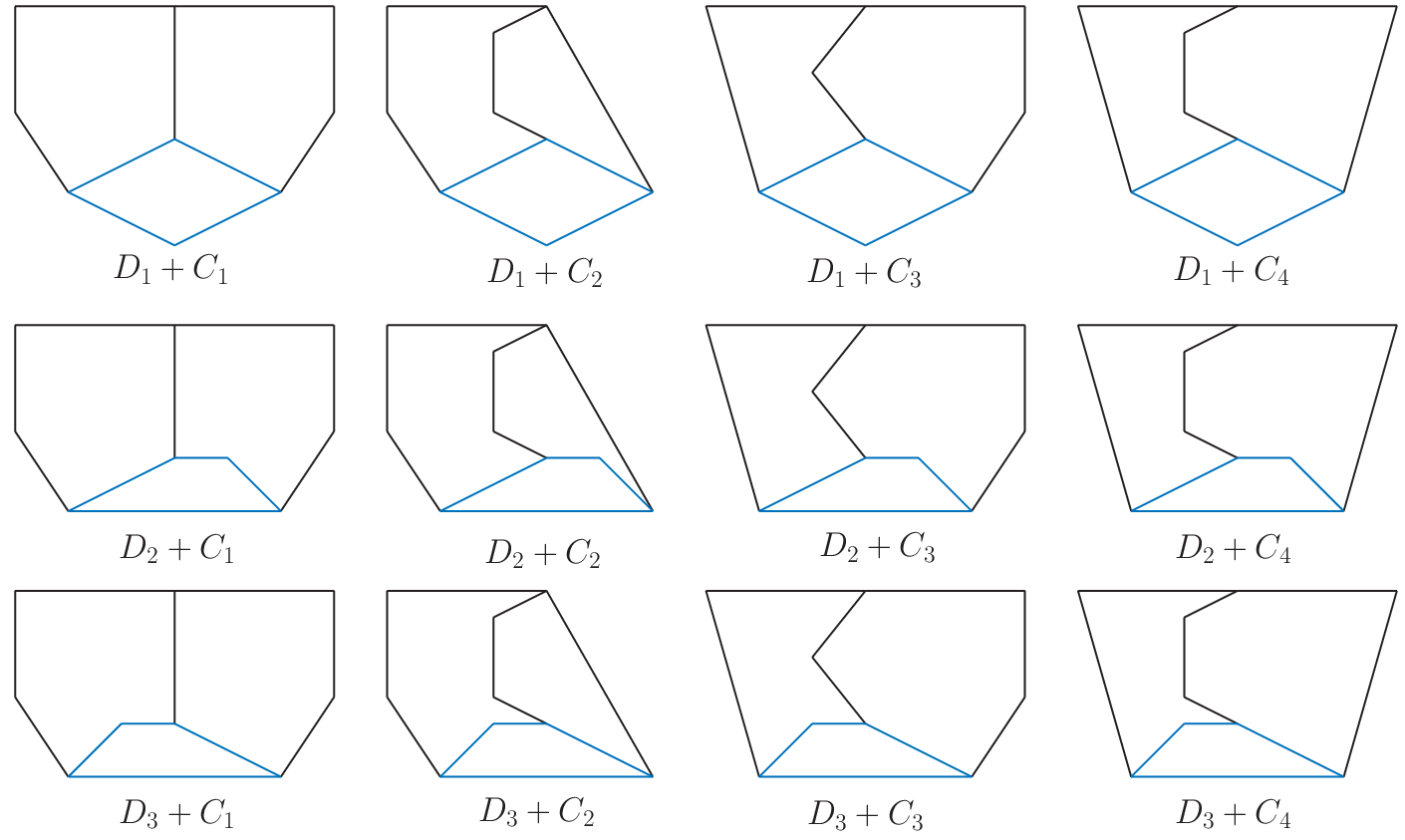
To finish this subsection, we present the results for Mercedes-logo type diagrams. By naively combining , there are in total twelve diagrams, as shown in Figure (6). The genus is given by
| 9 | 13 | 17 | 21 | |
| 13 | 13 | 17 | 17 | |
| 13 | 9 | 21 | 17 |
However, by loop momenta redefinition, we find that there are in fact only four different diagrams in Figure (6), denoted by as
Diagrams with the same genus in above table are the same diagram after loop momenta redefinition.
4.3 The derivation of formula
In order to have a general discussion, let us write the eleven equations of maximal unitarity cuts in a generic form. We always assume to have already reduced as many equations as possible to linear equations by algebraic manipulation of performing .
The four equations of box diagram can be expressed as
| (129) | |||
| (130) | |||
| (131) | |||
| (132) |
where , are the number of quadratic equations containing and respectively. Since the box diagram part contains four propagators, we have . The function
| (133) |
is a linear function of either or , since can take the value of one or zero, but they can not take the value of one simultaneously. Consequently, equation could be a linear function of either , or . Note that in our convention, there will always be a quadratic equation of , so . We keep it undefined just for generality.
The cut equations for two-loop diagram part can be expressed as
| (134) | |||
| (135) | |||
| (136) |
together with other four linear equations of .
The ramified points are defined by above seven equations of sub-two-loop part together with the discriminant of computed from box diagram part. It is a zero-dimensional ideal, and always has finite number of point solutions. Let us start from the analysis of discriminant. By solving three ’s with equations , we can write as a quadratic equation of remaining one variable . It is simple to compute the discriminant of this quadratic equation, although the explicit expression is too tedious to write down. The result takes the schematic form
| (137) |
where ’s are generic polynomials of with the degree dependence as shown in the argument. Note that we do not explicitly write down the dependence of lower degree monomials in ’s. It is clear that if
If other equations are general, then above information of dependence in is sufficient to determine the number of point solutions by convex hull polytope method. However, given the special form in (134), (135) and (136), there are non-trivial cancelation in we need to explore. The cancelation happens when . Naively, in this case is a degree four polynomial. All monomials of degree four in are given by
We can rewrite it as
So if , it reduces to a polynomial of degree two. Similarly, all monomials of degree three in can be rewritten as
So it can also be reduced to lower degree monomials provided . In this case, is actually a generic polynomial of degree two. The same cancelation happens for . All monomials of degree four in function can be rewritten as
So when considering , is a generic polynomial of degree three . The discriminant can at most be degree four when is or -dependent.
A further observation on shows that, the dependence of linear terms in are in fact not arbitrary. For example, when , in the quadratic polynomial , the eight linear terms have only four arbitrary pre-factors , and always appear together. It is the same for when , will always appear as one single item, and there are only four arbitrary pre-factors. Also in , we always have as a single item appearing in the linear equation. This observation leads to non-trivial reformulation for the discriminant when combined with equations , while is or -dependent. More explicitly, when and , the discriminant (137) becomes a polynomial of degree four, while the highest degree of is four and the highest degree of is two. If we redefine , then the discriminant can be rewritten as
It can be found that , so it vanishes in case that . The does not vanish individually, however the summation vanishes when combined with the equations . So finally the discriminant can be expressed as
Similarly, when , the discriminant can be expressed as
We have explored all the hidden structures in the discriminant under given equations in (134), (135) and (136). The degree dependence in is determined by and , and can be summarized as
| (138) |
For any given from cut equations of box diagram part, it is a degree four polynomial, and the degree dependence of and is explicitly shown. We want to emphasize that, is expressed as the above form such that at most two terms in or could appear at the same time. For all possible values of from cut equations, the discriminant can be
Then it is possible to compute the mixed volume of polytopes defined by polynomials . Naively, these polynomials are associated with 8-dimensional polytope, and it is not easy to compute the 8-dimensional volume. However, since there are four linear equations, we can solve four variables, and the remaining four equations are associated with 4-dimensional volume. It is still not easy to compute arbitrary 4-dimensional volume. But if we always choose to solve from four liner equations, then the remaining four variables are symmetric among or . Then we can treat or as a lattice line whose segment coordinate equals to the area of triangle in or -plane. An example is shown in the first diagram of Figure (7).

The length , , , etc. Instead of computing the 4-dimensional volume directly, we compute the 2-dimensional area but with a scaled coordinate. The polytope shown in the first diagram of Figure (7) then has area
Special attention should be paid to the case when discriminant is given by or . Because of the dependence of , we should treat as a variable. So when , we should transform the variables such that the discriminant become . Similarly, when , we should transform the variables such that the discriminant become . Then we can compute the 4-dimensional mixed volume accordingly. Let us take for example. In this case the discriminant is , so we do not need to transform variables. The solution of linear equations can be formally written as
In this case, the three quadratic equation , and become
The discriminant can be expressed as
The polytopes associated with these polynomials are plotted in Figure (7). is drawn explicitly with given for computation purpose, and the coordinate of vertices of polytopes are marked along the axes. Although these polytopes are plotted universally as triangles, we should note that they depend on the value of . For example, if , is a trapezoid. Given the four polytopes , , and with their coordinates, it is straightforward to draw the Minkowski sum among them. Then we can compute the mixed volume according to formula (163). We find that the mixed volume for is given by
| (139) |
Similarly, when , we have variables . The solution of linear equations are given by
In this case, we have
and . So the same computation shows that the mixed volume of four polytopes is given by
| (140) |
Finally, if , we have variables . The solution of linear equations is given by
In this case, we have
and . Then we get
| (141) |
Summarizing above discussions, we can express the number of ramified points, which equals to the mixed volume of four polytopes, as
which has already been shown in the beginning of this section.
5 More diagrams
5.1 The other three-loop diagrams
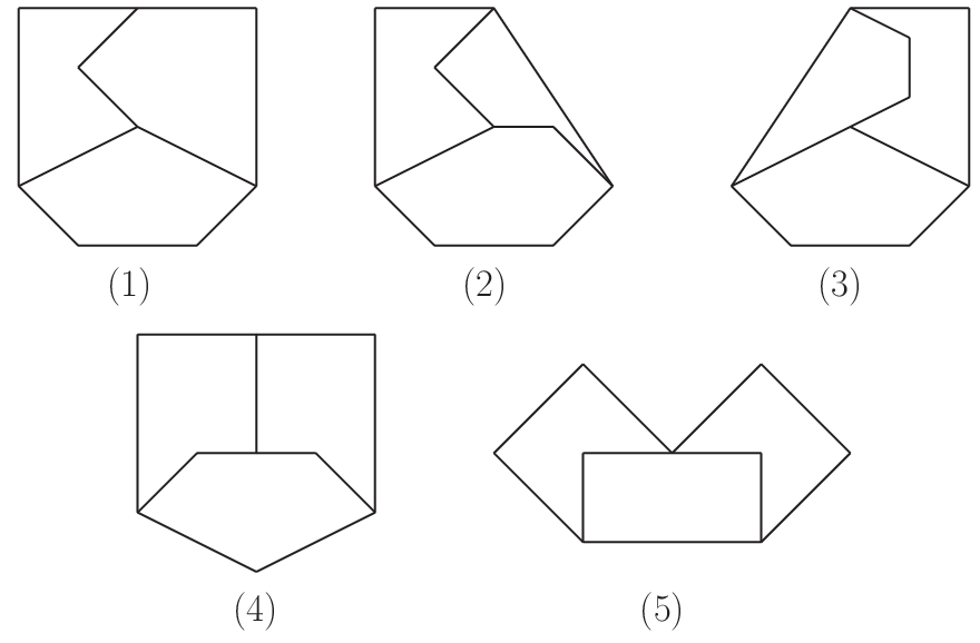
In previous section, we have presented a recursive formula for the study of genus of three-loop diagrams whose sub-two-loop diagram also defines a curve. There are still five diagrams which can not be included in this category. They are four Mercedes-logo type diagrams as shown in Figure (8.1) to Figure (8.4), and one ladder type diagram as shown in Figure (8.5). Since the sub-two-loop diagram or sub-one-loop diagram does not define curve, there is no covering map from the original curve to the curve of lower-loop diagram. Because of the highly complexity of algebraic system, it is quite difficult to compute the genus directly. Thus we introduce an algorithm to systematically study the genus based on numerical algebraic geometry. Given an algebraic system of maximal unitarity cuts of three-loop diagrams with arbitrary setup of numeric external momenta, it is possible to compute the genus within seconds by this algorithm. It also provides an opportunity of studying the global structure of maximal unitarity cuts of four-loop and even higher loop diagrams, where analytic study is almost impossible.
Let us apply the algorithm to the computation of five three-loop diagrams considered in this subsection. For each diagram, the corresponding polynomial system of maximal unitarity cuts defines an irreducible curve with each contribution for every and . Thus, Riemann-Hurwitz formula reduces to
By computing the degree of the curve and the number of branchpoints using numerical algebraic geometry via Bertini [73], we can obtain the genus by above formula,
- •
For diagram (8.1), we have , and , so the genus is .
- •
For diagram (8.2), we also have , but , so the genus is .
- •
For diagram (8.3), we have , and , so the genus is .
- •
Diagram (8.4) has the most complicated global structure among three-loop diagrams. The curve associated with this diagram has degree , and , so the genus is .
- •
For the last ladder type diagram (8.5), we have , and , so the genus is .
5.2 The White-house diagram

An interesting series of diagrams is shown in Figure (9) to any loop orders. If , we get the one-loop triangle diagram, which has . If , we get the two-loop double-box diagram, which has . The three-loop diagram is the first diagram resembling the White-house, and it has . Because of its resemblance between -loop and -loop diagrams, it is interesting to ask if we can compute the genus of -loop diagram from the information of -loop diagram. Define as the parametrization variables of the -th loop. From Figure (9) we can see that there are always two linear equations for each loop, so we can solve two variables in using these linear equations and get , where . Then we can compute the genus of -loop white-house diagram by Riemann-Hurwitz formula from the covering map
As usual, equations of box diagram part define a double covering map, and the ramified points have ramification index , determined by the discriminant equation for given points in curve . For the box diagram part, since , , the discriminant is given by . So the ramified points are determined by equations in variables in . It is easy to compute the number of ramified points for white-house diagrams. Since are two generic quadratic equations in two variables , by Bézout’s theorem, it has four distinct solutions. For each solution , equations are two generic equations in of degree one and two, so they have two solutions in . In total we get solutions in . Recursively, we get distinct solutions in . Above argument is based on the facts that different loops only share common propagators adjacently in a chain and the solution of linear equations only maps itself. So the Riemann-Hurwitz is given by
| (155) |
Given the first entry , it is not hard to solve above recursive formula and get
| (156) |
It indeed produces , , , and also an infinite series of genus such as , , , etc. The genus grows exponentially to infinity with the increasing of loops, which indicates the complexity of computation in higher-loop amplitudes.
6 Conclusion
To systematically study integrand reduction or integral reduction of multi-loop amplitudes via algebraic geometry method, the equations derived from propagators on-shell and their correspoinding variety (solution space) plays a very important role. These on-shell equations are the generating equations of ideal and Gröbner basis, which are the central objects in determining the set of independent integrand basis. The solution of each irreducible component of reducible ideal determines the parametrization of loop momenta, which greatly affects the evaluation of coefficients for integrand or integral basis. Thus, the study on the global structure of on-shell equations is the first step in the process of multi-loop reduction method, and provides a birds-eye view for further explicit computation.
In order to explicitly apply algebraic geometry method to the computation of three-loop integrand or integral reduction, it is necessary as an initial step to elaborate the global structure of the on-shell equations. Since a four-dimensional three-loop integral has twelve parametrization variables for loop momenta, the first category of non-trivial varieties is defined by on-shell equations of three-loop diagrams with eleven propagators. The ideal defined by these diagrams is complex one-dimensional, and it defines an algebraic curve, which is topological equivalent to a Riemann surface. The global structure is completely characterized by the geometric genus of the curve. Since these diagrams are the simplest three-loop diagrams with non-trivial solution space of on-shell equations, they would be the first candidate for applying algebraic geometric methods to the explicit computation of three-loop diagrams. Thus, a thorough study on the global structure of three-loop diagrams with eleven propagators can be served as a seed for the further computation of three-loop integrand and integral reduction.
In this paper, we provide a systematic study on the genus of curves defined by maximal unitarity cuts of three-loop diagrams with eleven propagators, generalizing the research in [55]. The Riemann-Hurwitz formula is used throughout the study. Among the 21 total diagrams. 16 diagrams have a sub-two-loop diagram whose equations of maximal unitarity cut also define curves. For these diagrams, the genus can be recursively computed from the genus of two-loop double-box and crossed-box diagrams together with the knowledge of ramified points. The recursive formula is given by
| (157) |
where
Note that above formula is general and independent of the convention of loop momenta. The number can be obtained by counting the number of corresponding propagators. Thus, the genus can be evaluated by just looking at the diagrams.
Besides, there are still five diagrams which can not be analyzed by the recursive formula from information of two-loop diagrams. For these diagrams, we implement an algorithm for the Riemann-Hurwitz formula based on numerical algebraic geometry. This algorithm also provides the possibility of studying more complicated algebraic system of four-loop or even higher loop diagrams in the future. It can also be applied to the analysis of the previous 16 diagrams, and we find that the results of the recursive formula and the algorithm agree.
The genus of 13 ladder type diagrams is given by
| Diagram | ![[Uncaptioned image]](1408.3355v2/A1S.png) |
![[Uncaptioned image]](1408.3355v2/A3S.png) |
![[Uncaptioned image]](1408.3355v2/A1D.png) |
![[Uncaptioned image]](1408.3355v2/A2S.png) |
![[Uncaptioned image]](1408.3355v2/A3D.png) |
![[Uncaptioned image]](1408.3355v2/B1D.png) |
![[Uncaptioned image]](1408.3355v2/B2S.png) |
![[Uncaptioned image]](1408.3355v2/B3D.png) |
![[Uncaptioned image]](1408.3355v2/B4S.png) |
![[Uncaptioned image]](1408.3355v2/A2D.png) |
![[Uncaptioned image]](1408.3355v2/B2D.png) |
![[Uncaptioned image]](1408.3355v2/B4D.png) |
![[Uncaptioned image]](1408.3355v2/Ex5.png) |
|---|---|---|---|---|---|---|---|---|---|---|---|---|---|
| Genus | 5 | 5 | 9 | 9 | 9 | 13 | 13 | 13 | 13 | 17 | 21 | 21 | 33 |
The genus of 8 Mercedes-logo type diagrams is given by
| Diagram | ![[Uncaptioned image]](1408.3355v2/D1C1.png) |
![[Uncaptioned image]](1408.3355v2/D1C2.png) |
![[Uncaptioned image]](1408.3355v2/D1C3.png) |
![[Uncaptioned image]](1408.3355v2/D1C4.png) |
![[Uncaptioned image]](1408.3355v2/Ex3.png) |
![[Uncaptioned image]](1408.3355v2/Ex1.png) |
![[Uncaptioned image]](1408.3355v2/Ex2.png) |
![[Uncaptioned image]](1408.3355v2/Ex4.png) |
|---|---|---|---|---|---|---|---|---|
| Genus | 9 | 13 | 17 | 21 | 29 | 33 | 45 | 55 |
In general terms, the higher the genus is, the more complicated the algebraic system will be. So, a first direct application of above result would be the judgement of the complexity of three-loop diagrams we would like to evaluate. Different from two-loop diagrams where the highest genus is only three, the genus for three-loop diagrams can be as high as 55. This indicates highly complex nature of three-loop diagrams compared to two-loop diagrams. Curves of different diagrams with the same genus are topological equivalent to each other, we expect that this equivalence would also play a role in relating those different diagrams.
We also present an example beyond three-loop diagrams, by
generalizing the simplest white-house diagram
to any loops. The genus of
-loop white-house diagram is
Hence, , , , etc. In particular, it is possible for the genus to grow without bound. Interestingly, the genus of -loop white-house diagram equals to the genus of -dimensional hypercube. This relates the algebraic system of maximal unitarity cuts of multi-loop diagrams directly to well-known geometric objects.
An interesting phenomenon is observed in [55] that the genus is always an odd integer. This is further verified by results presented here. We can claim that the genus of curve defined by maximal unitarity cuts of any multi-loop diagrams is an odd integer. This can be shown by looking at the on-shell equations of degenerate limit where one external momentum is massless. Assuming that after solving linear equations, the algebraic curve is given by with variables. It is always possible to take one external momentum as massless, and the corresponding quadratic equation factorizes as , where are linear. The linear polynomials are two equivalent branches of quadratic polynomial , and ideal can be primary decomposed into two equivalent irreducible ideals and . So, the genus of curve defined by equals to the genus of the curve defined by . If there are intersecting points between two curves, then the genus of original curve defined by is given by . The number is in fact the number of distinct solutions of zero-dimensional ideal . In projective space, according to Bézout’s theorem, is given by the products of degree of each polynomial in , which is an even integer. This guarantees that the genus is an odd integer, and explains the puzzle in [55].
As we have mentioned, information of global structure of on-shell equations is the first step to the integrand or integral reduction of multi-loop integrals. The genus is a powerful concept that connects the algebraic system of maximal unitarity cuts to geometric objects, as hinted in the White-house example. Since so far only a few explicit computation of three-loop integral reduction is done, we still need to wait for more three-loop examples to reveal the connection and also the possible equivalence of different diagrams with the same genus. With the algorithm based on numerical algebraic geometry presented in this paper, it is possible to work out the global structure of curves defined by maximal unitarity cuts of four-loop diagrams. However, this information is not urgent, since integrand or integral reduction of four-loop integral is still far from practice. We hope that in future there will be more results of three-loop integrand reduction showing up, so that we can clarify the underlining power of genus. Then it can be similarly generalized to higher loop diagrams.
The global structure of higher-dimensional varieties, defined by the maximal unitarity cuts of -loop diagram with propagators, is still unclear even for two-loop diagrams. This information is important for the computation of two-loop diagrams besides double-box and crossed-box. We hope that both computational and numerical algebraic geometry can play a similar role in the analysis of global structure for those diagrams in the future.
Acknowledgements.
We would like to thank Simon Caron-Huot, David Kosower, and Michael Stillman for useful discussion. RH would like to thank the Niels Bohr International Academy and Discovery Center, the Niels Bohr Institute for its hospitality. The work of YZ is supported by Danish Council for Independent Research (FNU) grant 11-107241. RH’s research is supported by the European Research Council under Advanced Investigator Grant ERC-AdG-228301. DM was supported by a DARPA YFA. JDH was supported by a DARPA YFA and NSF DMS-1262428.Appendix A Solving polynomial equations using convex polytope
An algebraic system of polynomial equations in variables is expected to define a zero-dimensional ideal. When , if the algebraic system has finite many zeros in , then Bézout’s theorem states that the number of zeros is at most . Generalization to arbitrary polynomial equations can be similarly understood. If there are finitely many zeros in for , then the upper bound on the number of solutions is , which is sharp for generic polynomials. For sparse polynomials, this bound is typically not sharp. For illustration, we take a similar example given in [74]. The two polynomials
| (158) |
have four distinct zeros in for generic coefficients ’s. However, Bézout’s theorem provides an upper bound of . In order to predict the actual number 4 instead of 6, we need to go from Bézout’s theorem to Bernstein’s theorem. Bernstein’s theorem states that for two bivariate polynomials and , the number of zeros in is bounded above by the mixed area of the two corresponding Newton polytopes . Here, . To understand this theorem, one should first associate a convex polytope to polynomial. A polytope is a subset of which is the convex hull of a finite size of points. For example, in , the convex hull is a square. For a given polynomial
we can associate a Newton convex polytope
| (159) |
Since ’s are always non-negative integers, it is a lattice convex polytope. Given two polytopes , the Minkowski sum is given by
| (160) |
Then the mixed area is given by
| (161) |
We can apply the convex polytope method to the example polynomials (158), which is shown in Figure (10).

The mixed area is given by
Following Bernstein’s theorem, the number of zeros for with general coefficients in is exactly . In case, the bound can be trivially lifted from to . One remark is that, in computing the mixed area, the two polynomials should be independent. For example, two polynomials , have the same zeros as . However, if we include the vanishing term in as vertices in polytope , then we get the wrong result. Before computing the area, we should remove the redundant terms such as in .
Bernstein’s theorem can be generalized to higher dimension. The number of solutions in of polynomials in variables is bounded above by the mixed volume of Newton polytopes. The mixed volume of in is given by formula
| (162) |
where is a non-empty subsets of and is the length of . The volume is Euclidean volume in . For example, in , the mixed volume is
| (163) | |||||
References
- [1] L.M. Brown and R.P. Feynman. Radiative corrections to Compton scattering. Phys.Rev., 85:231–244, 1952.
- [2] G. Passarino and M.J.G. Veltman. One Loop Corrections for e+ e- Annihilation Into mu+ mu- in the Weinberg Model. Nucl.Phys., B160:151, 1979.
- [3] Gerard ’t Hooft and M.J.G. Veltman. Scalar One Loop Integrals. Nucl.Phys., B153:365–401, 1979.
- [4] Robin G. Stuart. Algebraic Reduction of One Loop Feynman Diagrams to Scalar Integrals. Comput.Phys.Commun., 48:367–389, 1988.
- [5] Robin G. Stuart and A. Gongora. Algebraic Reduction of One Loop Feynman Diagrams to Scalar Integrals. 2. Comput.Phys.Commun., 56:337–350, 1990.
- [6] L.D. Landau. On analytic properties of vertex parts in quantum field theory. Nucl.Phys., 13:181–192, 1959.
- [7] S. Mandelstam. Determination of the pion - nucleon scattering amplitude from dispersion relations and unitarity. General theory. Phys.Rev., 112:1344–1360, 1958.
- [8] Stanley Mandelstam. Analytic properties of transition amplitudes in perturbation theory. Phys.Rev., 115:1741–1751, 1959.
- [9] R.E. Cutkosky. Singularities and discontinuities of Feynman amplitudes. J.Math.Phys., 1:429–433, 1960.
- [10] Zvi Bern, Lance J. Dixon, David C. Dunbar, and David A. Kosower. One loop n point gauge theory amplitudes, unitarity and collinear limits. Nucl.Phys., B425:217–260, 1994.
- [11] Zvi Bern, Lance J. Dixon, David C. Dunbar, and David A. Kosower. Fusing gauge theory tree amplitudes into loop amplitudes. Nucl.Phys., B435:59–101, 1995.
- [12] Z. Bern and A.G. Morgan. Massive loop amplitudes from unitarity. Nucl.Phys., B467:479–509, 1996.
- [13] Ruth Britto, Freddy Cachazo, and Bo Feng. New recursion relations for tree amplitudes of gluons. Nucl.Phys., B715:499–522, 2005.
- [14] Ruth Britto, Freddy Cachazo, Bo Feng, and Edward Witten. Direct proof of tree-level recursion relation in Yang-Mills theory. Phys.Rev.Lett., 94:181602, 2005.
- [15] Ruth Britto, Evgeny Buchbinder, Freddy Cachazo, and Bo Feng. One-loop amplitudes of gluons in SQCD. Phys.Rev., D72:065012, 2005.
- [16] Charalampos Anastasiou, Ruth Britto, Bo Feng, Zoltan Kunszt, and Pierpaolo Mastrolia. D-dimensional unitarity cut method. Phys.Lett., B645:213–216, 2007.
- [17] Charalampos Anastasiou, Ruth Britto, Bo Feng, Zoltan Kunszt, and Pierpaolo Mastrolia. Unitarity cuts and Reduction to master integrals in d dimensions for one-loop amplitudes. JHEP, 0703:111, 2007.
- [18] Ruth Britto, Freddy Cachazo, and Bo Feng. Generalized unitarity and one-loop amplitudes in N=4 super-Yang-Mills. Nucl.Phys., B725:275–305, 2005.
- [19] Zvi Bern, Lance J. Dixon, and David A. Kosower. One loop amplitudes for e+ e- to four partons. Nucl.Phys., B513:3–86, 1998.
- [20] Giovanni Ossola, Costas G. Papadopoulos, and Roberto Pittau. Reducing full one-loop amplitudes to scalar integrals at the integrand level. Nucl.Phys., B763:147–169, 2007.
- [21] Darren Forde. Direct extraction of one-loop integral coefficients. Phys.Rev., D75:125019, 2007.
- [22] R. Keith Ellis, W.T. Giele, and Z. Kunszt. A Numerical Unitarity Formalism for Evaluating One-Loop Amplitudes. JHEP, 0803:003, 2008.
- [23] William B. Kilgore. One-loop Integral Coefficients from Generalized Unitarity. 2007.
- [24] Walter T. Giele, Zoltan Kunszt, and Kirill Melnikov. Full one-loop amplitudes from tree amplitudes. JHEP, 0804:049, 2008.
- [25] Giovanni Ossola, Costas G. Papadopoulos, and Roberto Pittau. On the Rational Terms of the one-loop amplitudes. JHEP, 0805:004, 2008.
- [26] S.D. Badger. Direct Extraction Of One Loop Rational Terms. JHEP, 0901:049, 2009.
- [27] Janusz Gluza, Krzysztof Kajda, and David A. Kosower. Towards a Basis for Planar Two-Loop Integrals. Phys.Rev., D83:045012, 2011.
- [28] Yang Zhang. Integrand-Level Reduction of Loop Amplitudes by Computational Algebraic Geometry Methods. JHEP, 1209:042, 2012.
- [29] Pierpaolo Mastrolia, Edoardo Mirabella, Giovanni Ossola, and Tiziano Peraro. Scattering Amplitudes from Multivariate Polynomial Division. Phys.Lett., B718:173–177, 2012.
- [30] Simon Badger, Hjalte Frellesvig, and Yang Zhang. Hepta-Cuts of Two-Loop Scattering Amplitudes. JHEP, 1204:055, 2012.
- [31] Bo Feng and Rijun Huang. The classification of two-loop integrand basis in pure four-dimension. JHEP, 1302:117, 2013.
- [32] Ronald H.P. Kleiss, Ioannis Malamos, Costas G. Papadopoulos, and Rob Verheyen. Counting to One: Reducibility of One- and Two-Loop Amplitudes at the Integrand Level. JHEP, 1212:038, 2012.
- [33] Simon Badger, Hjalte Frellesvig, and Yang Zhang. An Integrand Reconstruction Method for Three-Loop Amplitudes. JHEP, 1208:065, 2012.
- [34] Pierpaolo Mastrolia, Edoardo Mirabella, Giovanni Ossola, and Tiziano Peraro. Integrand-Reduction for Two-Loop Scattering Amplitudes through Multivariate Polynomial Division. Phys.Rev., D87(8):085026, 2013.
- [35] Pierpaolo Mastrolia, Edoardo Mirabella, Giovanni Ossola, Tiziano Peraro, and Hans van Deurzen. The Integrand Reduction of One- and Two-Loop Scattering Amplitudes. PoS, LL2012:028, 2012.
- [36] Pierpaolo Mastrolia, Edoardo Mirabella, Giovanni Ossola, and Tiziano Peraro. Multiloop Integrand Reduction for Dimensionally Regulated Amplitudes. Phys.Lett., B727:532–535, 2013.
- [37] Simon Badger, Hjalte Frellesvig, and Yang Zhang. A Two-Loop Five-Gluon Helicity Amplitude in QCD. JHEP, 1312:045, 2013.
- [38] Hans van Deurzen, Gionata Luisoni, Pierpaolo Mastrolia, Edoardo Mirabella, Giovanni Ossola, et al. Multi-leg One-loop Massive Amplitudes from Integrand Reduction via Laurent Expansion. JHEP, 1403:115, 2014.
- [39] F.V. Tkachov. A Theorem on Analytical Calculability of Four Loop Renormalization Group Functions. Phys.Lett., B100:65–68, 1981.
- [40] K.G. Chetyrkin and F.V. Tkachov. Integration by Parts: The Algorithm to Calculate beta Functions in 4 Loops. Nucl.Phys., B192:159–204, 1981.
- [41] S. Laporta. Calculation of master integrals by difference equations. Phys.Lett., B504:188–194, 2001.
- [42] S. Laporta. High precision calculation of multiloop Feynman integrals by difference equations. Int.J.Mod.Phys., A15:5087–5159, 2000.
- [43] Bo Feng, Jun Zhen, Rijun Huang, and Kang Zhou. Integral Reduction by Unitarity Method for Two-loop Amplitudes: A Case Study. JHEP, 1406:166, 2014.
- [44] Johannes M. Henn. Multiloop integrals in dimensional regularization made simple. Phys.Rev.Lett., 110(25):251601, 2013.
- [45] Simon Caron-Huot and Johannes M. Henn. Iterative structure of finite loop integrals. JHEP, 1406:114, 2014.
- [46] David A. Kosower and Kasper J. Larsen. Maximal Unitarity at Two Loops. Phys.Rev., D85:045017, 2012.
- [47] Kasper J. Larsen. Global Poles of the Two-Loop Six-Point N=4 SYM integrand. Phys.Rev., D86:085032, 2012.
- [48] Simon Caron-Huot and Kasper J. Larsen. Uniqueness of two-loop master contours. JHEP, 1210:026, 2012.
- [49] Henrik Johansson, David A. Kosower, and Kasper J. Larsen. Two-Loop Maximal Unitarity with External Masses. Phys.Rev., D87:025030, 2013.
- [50] Mads Sogaard. Global Residues and Two-Loop Hepta-Cuts. JHEP, 1309:116, 2013.
- [51] Henrik Johansson, David A. Kosower, and Kasper J. Larsen. Maximal Unitarity for the Four-Mass Double Box. Phys.Rev., D89:125010, 2014.
- [52] Mads Sogaard and Yang Zhang. Multivariate Residues and Maximal Unitarity. JHEP, 1312:008, 2013.
- [53] Mads Sogaard and Yang Zhang. Unitarity Cuts of Integrals with Doubled Propagators. JHEP, 1407:112, 2014.
- [54] Mads Sogaard and Yang Zhang. Massive Nonplanar Two-Loop Maximal Unitarity. 2014.
- [55] Rijun Huang and Yang Zhang. On Genera of Curves from High-loop Generalized Unitarity Cuts. JHEP, 1304:080, 2013.
- [56] Daniel J. Bates, Jonathan D. Hauenstein, Andrew J. Sommese, and Charles W. Wampler. Numerically solving polynomial systems with Bertini, volume 25 of Software, Environments, and Tools. Society for Industrial and Applied Mathematics (SIAM), Philadelphia, PA, 2013.
- [57] Dhagash Mehta, Yang-Hui He, and Jonathan D. Hauenstein. Numerical Algebraic Geometry: A New Perspective on String and Gauge Theories. JHEP, 1207:018, 2012.
- [58] R. Hartshorne. Algebraic Geometry. Graduate Texts in Mathematics. Springer, 1977.
- [59] C. Maclean and D. Perrin. Algebraic Geometry: An Introduction. Universitext. Springer, 2007.
- [60] Daniel J. Bates, Chris Peterson, Andrew J. Sommese, and Charles W. Wampler. Numerical computation of the genus of an irreducible curve within an algebraic set. J. Pure Appl. Algebra, 215(8):1844–1851, 2011.
- [61] Jonathan D. Hauenstein and Andrew J. Sommese. Membership tests for images of algebraic sets by linear projections. Appl. Math. Comput., 219(12):6809–6818, 2013.
- [62] Andrew J. Sommese and Charles W. Wampler, II. The numerical solution of systems of polynomials. World Scientific Publishing Co. Pte. Ltd., Hackensack, NJ, 2005. Arising in engineering and science.
- [63] Dhagash Mehta. Numerical Polynomial Homotopy Continuation Method and String Vacua. Adv.High Energy Phys., 2011:263937, 2011.
- [64] Jonathan Hauenstein, Yang-Hui He, and Dhagash Mehta. Numerical elimination and moduli space of vacua. JHEP, 1309:083, 2013.
- [65] Jonathan D. Hauenstein and Charles W. Wampler. Isosingular sets and deflation. Found. Comput. Math., 13(3):371–403, 2013.
- [66] Jonathan D. Hauenstein, Andrew J. Sommese, and Charles W. Wampler. Regeneration homotopies for solving systems of polynomials. Math. Comp., 80(273):345–377, 2011.
- [67] Jonathan D. Hauenstein, Andrew J. Sommese, and Charles W. Wampler. Regenerative cascade homotopies for solving polynomial systems. Appl. Math. Comput., 218(4):1240–1246, 2011.
- [68] Daniel J. Bates, Jonathan D. Hauenstein, Chris Peterson, and Andrew J. Sommese. A numerical local dimensions test for points on the solution set of a system of polynomial equations. SIAM J. Numer. Anal., 47(5):3608–3623, 2009.
- [69] Andrew J. Sommese, Jan Verschelde, and Charles W. Wampler. Symmetric functions applied to decomposing solution sets of polynomial systems. SIAM J. Numer. Anal., 40(6):2026–2046, 2002.
- [70] Jonathan D. Hauenstein and Charles W Wampler. Numerical algebraic intersection using regeneration. 2013.
- [71] Daniel J. Bates, Daniel A. Brake, Jonathan D. Hauenstein, Andrew J. Sommese, and Charles W. Wampler. Homotopies to compute points on connected components. Preprint, 2014.
- [72] Daniel R. Grayson and Michael E. Stillman. Macaulay2, a software system for research in algebraic geometry. Available at http://www.math.uiuc.edu/Macaulay2/.
- [73] Daniel J. Bates, Jonathan D. Hauenstein, Andrew J. Sommese, and Charles W. Wampler. Bertini: Software for numerical algebraic geometry. Available at http://bertini.nd.edu.
- [74] Bernd Sturmfels. Solving systems of polynomial equations, volume 97. American Mathematical Soc.