Improving the distance reduction step in the von Neumann algorithm

C.H. Jeffrey Pang Current address: Department of Mathematics
National University of Singapore
Block S17 08-11
10 Lower Kent Ridge Road
Singapore 119076 Email address: matpchj@nus.edu.sg

Date: August 24, 2026

Abstract.

A known first order method to find a feasible solution to a conic problem is an adapted von Neumann algorithm. We improve the distance reduction step there by projecting onto the convex hull of previously generated points using a primal active set quadratic programming (QP) algorithm. The convergence theory is improved when the QPs are as large as possible. For problems in $\mathbb{R}^{2}$ , we analyze our algorithm by epigraphs and the monotonicity of subdifferentials. Logically, the larger the set to project onto, the better the performance per iteration, and this is indeed seen in our numerical experiments.

Key words and phrases:

von Neumann algorithm, perceptron algorithm, active set, quadratic programming.

2010 Mathematics Subject Classification

90C25, 90C20, 90C60, 49N15, 49J53, 52A20

1. Introduction

For $A\in\mathbb{R}^{m\times n}$ , consider the linear inequality system

(1.1a)		$A^{T}y>0,$
and its alternative
(1.1b)		$Ax=0,\mathbf{1}^{T}x=1\mbox{ and }x\geq 0,$

where $\mathbf{1}$ stands for the vector of all ones. More generally, for a closed convex cone $K\subset\mathbb{R}^{n}$ with interior, consider the conic system

(1.2a)		$A^{T}y\in\mbox{\rm int}(K^{*}),$
and its alternative
(1.2b)		$Ax=0,\bar{u}^{T}x=1\mbox{ and }x\in K.$

where $K^{*}:=\{z:z^{T}x\geq 0\mbox{ for all }x\in K\}$ is the (positive) dual cone of $K$ and $\bar{u}$ is some point in $\mbox{\rm int}(K^{*})$ . It is easy to see that (1.1) is the particular case of (1.2) when $K=\mathbb{R}_{+}^{n}$ and $\bar{u}=\mathbf{1}$ . An easy variant of Farkas’s Lemma shows that exactly one of (1.1a) and (1.1b) is feasible. A similar result is easily seen to hold for (1.2).

The perceptron algorithm is a simple iterative algorithm that finds a solution to system (1.1a) if it is feasible. The von Neumann algorithm is a simple iterative algorithm that finds an approximate solution to (1.1b) if it is feasible, and it can give a solution $y$ to (1.1a) if (1.1b) turns out to be infeasible.

We recall some of the history of the perceptron and von Neumann algorithms. The perceptron algorithm was introduced in [Ros58] for solving classification problems in machine learning. The von Neumann algorithm was privately communicated by von Neumann to Dantzig in the late 1940s, and later studied by Dantzig [Dan92a, Dan92b]. Block [Blo62] and Novikoff [Nov62] showed that when (1.1a) is feasible, the perceptron algorithm finds a solution to (1.1a) after at most $1/[\rho(A)]^{2}$ iterations, where $\rho(A)$ , a condition number defined in [CC01], is defined by

\rho(A):=\left|\max_{\|y\|_{2}=1}\min_{j=1,\dots,n}\frac{a_{j}^{T}y}{\|a_{j}\|_{2}}\right|.

When (1.1a) is feasible, $\rho(A)$ is precisely the width of the feasibility cone $\{y:A^{T}y\geq 0\}$ as defined in [FV99]. This condition number traces its roots to [Ren95a] (see also [Ren95b, PR00]). Epelman and Freund [EF00] showed that the von Neumann algorithm either computes an $\epsilon$ -solution to (1.1b) in $O(\frac{1}{\rho(A)^{2}}\log(\frac{1}{\epsilon}))$ iterations when (1.1b) is feasible, or finds a solution to the alternative system (1.1a) in $O(1/\rho(A)^{2})$ iterations if (1.1a) is feasible. They also treated the generalized pair (1.2). (See also [EF02].)

Consider the problem

(1.3)	$\displaystyle\min_{x\in\mathbb{R}^{n}}$	$\displaystyle\frac{1}{2}\\|Ax\\|^{2}$
	s.t.	$\displaystyle\bar{u}^{T}x=1$
		$\displaystyle x\in K.$

It is clear that (1.2b) is feasible if and only if the objective value of (1.3) is zero. Alternatives for solving (1.2) include the interior point algorithm and the ellipsoid algorithm. Both the interior point and ellipsoid methods are sophisticated algorithms that give a better complexity bound, but require significant computational effort to perform each iteration.

For the case where $K=\mathbb{R}_{+}^{n}$ and $\bar{u}=\mathbf{1}$ , an active set quadratic programming (QP) algorithm can also be an alternative. An active set QP algorithm can easily solve (1.1) if $m$ and $n$ are small, and the subproblems in each iteration are easily solved when $m$ is small. For larger problems, an active set QP algorithm is considered to be as efficient as the simplex method in practice. An advantage of the active set QP method is that the minimum of (1.3) can be attained in finitely many iterations. If the active set QP algorithm is used to find a feasible solution to (1.1a), the algorithm can terminate before the minimizer is found.

The perceptron and von Neumann algorithms are a first-order methods for solving (1.1) in that the computational effort in each iteration is small, but one would need much more iterations than a more sophisticated algorithm like the interior point method or the ellipsoid method. For large scale problems, a first-order method may be the only reasonable approach. Since the von Neumann algorithm uses only matrix vector multiplications and do not solve linear systems, it is also useful for sparse problems.

Problem (1.1b) is a particular case of the problem of finding whether the convex hulls of two sets of points overlap. More precisely, for $A\in\mathbb{R}^{m\times n_{1}}$ and $B\in\mathbb{R}^{m\times n_{2}}$ , consider

(1.4)	$\displaystyle\min_{x\in\mathbb{R}^{n_{1}},z\in\mathbb{R}^{n_{2}}}$	$\displaystyle\frac{1}{2}\\|Ax-Bz\\|^{2}$
	s.t.	$\displaystyle\mathbf{1}^{T}x=1$
		$\displaystyle\mathbf{1}^{T}z=1$
		$\displaystyle x,z\geq 0.$

The sets are the vectors spanned by the columns of $A$ and $B$ respectively. When $B$ is the zero vector of size $m\times 1$ , then (1.4) reduces to to (1.3). When the convex hull of these two sets of points do not overlap, the classification problem is the problem of finding a good separating hyperplane between these two sets. Research in the classification problem has gone on to handle the misclassifications of some of the points [Sch06].

There are other accelerations of the perceptron and von Neumann algorithms in the literature. A smoothed perceptron von Neumann algorithm was studied in [SP12], who were in turn motivated by the smoothing techniques in [Nes05]. A randomized rescaled version of the perceptron algorithm was proposed in [DV06] that terminates in $O(m\log(\frac{1}{\rho(A)}))$ with high probability. The randomized algorithm was extended to more general conic systems in [BFV09].

Another well-known algorithm for solving feasibility problems is the method of alternating projections. The idea of using a QP as an intermediate step to accelerate the method of alternating projections was studied by the author for general feasibility problems in [Pan14b, Pan13, Pan14a], though the idea had been studied for particular cases in [Pie84, BCK06] (intersection of an affine space and a halfspace), [GP98, GP01] (under smoothness conditions) and [Fuk82] (for the convex inequality problem). For more information, we refer to the references in the papers mentioned earlier, and highlight [BB96, ER11] as well as [BZ05, Subsubsection 4.5.4] for more information about the theory and method of alternating projections. It is natural to ask whether a QP can accelerate algorithms for solving (1.1) and (1.2).

1.1. Contributions of this paper

We make use of the fact that it is relatively easy to project a point onto the convex hull of a small number of points using an active set QP algorithm to generalize the von Neumann algorithm. When the size of the set that defines the convex hull to be projected on equals two, then our algorithm becomes the setting of the von Neumann algorithm. The size of this set can be chosen to be as large as one can reasonably can to increase efficiency, as long as each iteration is still manageable. (See lines 7-10 of Algorithm 2.1, Remark 2.3 and the subsequent discussion.)

For the case of (1.1), the generalized algorithm (Algorithm 2.1) is a variant of an active set QP algorithm, and it converges to a point in finitely many iterations to find a $y$ satisfying (1.1a) or an $x$ satisfying (1.1b), whichever one is feasible.

For the case of (1.2), Theorem 3.3 proves that Algorithm 2.1 converges to a point in finitely many iterations if $0\in\mbox{\rm int}(S)$ , where $S=\mbox{\rm int}\{Ap:\bar{u}^{T}p=1,p\in K\}$ , and all previously identified points are kept. For the case when $m=2$ and $0$ is on the boundary of $S$ , we show that the convergence of $\{\|y_{i}\|\}_{i}$ in Algorithm 2.1 to zero is linear with rate at worst $1/\sqrt{2}$ in Theorem 3.6, and further analyze the behavior of Algorithm 2.1 in Section 4 by appealing to epigraphs and the monotonicity of subdifferentials.

1.2. Notation

We list down some common notation used in this paper, which are rather standard material in convex analysis [Roc70]. Let $C\subset\mathbb{R}^{n}$ be a set.

$\mbox{\rm aff}(C)$

The affine hull of the set $C$ .
$\mbox{\rm conv}(C)$

The convex hull of the set $C$ .

If $C$ is a closed convex set, we have the following notation.

$T_{C}(x)$

The tangent cone of the set $C$ at $x$ .
$\partial C$

The boundary of $C$ .

For a convex function $f:\mathbb{R}\to\mathbb{R}$ , we have the following notation.

$\partial f(x)$

The subdifferential of $f$ at $x$ , and $\partial f(x)$ is a subset of $\mathbb{R}$ .

2. Algorithm

In this section, we propose Algorithm 2.1 for solving (1.2), and describe the algorithmic issues incrementally. We start by describing Algorithm 2.1.

Algorithm 2.1.

(Algorithm for system (1.2)) For $A\in\mathbb{R}^{m\times n}$ and a closed convex cone $K\subset\mathbb{R}^{n}$ with interior, this algorithm finds either a $y\in\mathbb{R}^{m}$ satisfying (1.2a) or an $x\in\mathbb{R}^{n}$ satisfying (1.2b).

01 Set $x_{0}=p_{0}\in\{x:\bar{u}^{T}x=1,x\in K\}$ , $y_{0}=Ax_{0}$ and $i=0$

02 Loop

03 Find some $p_{i+1}$ such that $p_{i+1}\in K$ , $\bar{u}^{T}p_{i+1}=1$ and $p_{i+1}^{T}Ay_{i}\leq 0$ .

04 If $p^{T}A^{T}y_{i}>0$ for all $p\in K$ such that $\bar{u}^{T}p=1$ ,

05 then $A^{T}y_{i}\in\mbox{\rm int}(K^{*})$ , solving (1.2a), so we exit.

06 (Distance reduction)

07 Let $C_{i+1}=\{Ac_{i+1,1},\dots,Ac_{i+1,k_{i+1}}\}$ be a finite subset of

08 $\mbox{\rm conv}\{Ap_{0},Ap_{1},\dots,Ap_{i+1}\}$ .

09 Let $y_{i+1}:=P_{\scriptsize\mbox{\rm conv}(\tilde{C})}(0)=\sum_{j=1}^{k_{i+1}}\lambda_{j}^{(i+1)}Ac_{i+1,j}$ , where $\tilde{C}\subset C_{i+1}$ ,

10 $\sum_{j=1}^{k_{i+1}}\lambda_{j}^{(i+1)}=1$ and $\lambda_{j}^{(i+1)}\geq 0$ for all $j\in\{1,\dots,k_{i+1}\}$ .

11 Let $x_{i+1}=\sum_{j=1}^{k_{i+1}}\lambda_{j}^{(i+1)}c_{i+1,j}$ , and $i\leftarrow i+1$ .

12 Perform an aggregation step to reduce the size of $C_{i}$ .

13 until $\|y_{i}\|=\|Ax_{i}\|$ small.

Remark 2.2.

(Choice of $p_{i+1}$ ) The $p_{i+1}$ in line 3 is typically chosen by solving the conic section optimization problem

(2.1)	$\displaystyle p_{i+1}=$	$\displaystyle\arg\min_{p}$	$\displaystyle p^{T}A^{T}y_{i}$
		s.t.	$\displaystyle\bar{u}^{T}p=1$
			$\displaystyle p\in K.$

In the case where $\bar{u}=\mathbf{1}$ and $K=\mathbb{R}_{+}^{n}$ , the vector $p_{i+1}$ is easily seen to be the elementary vector $e_{j}$ , where $j$ corresponds to the coordinate of $A^{T}y_{i}$ with the minimum value. In the case where $K$ is the semidefinite cone $\mathcal{S}_{+}^{k\times k}$ and $\bar{u}$ is the identity matrix in $\mathbb{R}^{k\times k}$ , the optimization objective is now $\langle p,A^{T}y_{i}\rangle$ , where $A^{T}$ is the adjoint of the operator $A:\mathcal{S}_{+}^{k\times k}\to\mathbb{R}^{m}$ and $\langle,\rangle$ corresponds to the trace inner product. A minimizer of (2.1) is easily obtained once the eigenvalue factorization of $A^{T}y_{i}$ is obtained. If $K$ is the direct sum of sets of the form $\mathbb{R}_{+}^{n}$ and semidefinite cones, the problem (2.1) can still be easily solved. More elaboration is given in [EF00] for example.

We show that Algorithm 2.1 is an enhancement to the von Neumann algorithm.

Remark 2.3.

(von Neumann algorithm) The generalized von Neumann algorithm to solve (1.2) in [EF00] is a particular case of Algorithm 2.1 when the $p_{i+1}$ in line 3 is chosen by (2.1) and, most importantly, the set $C_{i+1}$ in line 7 is chosen to be $\{y_{i},Ap_{i+1}\}$ . Choices of $p_{i+1}$ different from (2.1) were explored. See for example [SP13]. The classical von Neumann algorithm is the particular case when $K=\mathbb{R}_{+}^{n}$ , $\bar{u}=\mathbf{1}$ , $p_{0}=\frac{1}{n}\mathbf{1}$ . When $K$ is a product of semidefinite cones and cones of the type $\mathbb{R}_{+}^{k}$ , the optimization problem (2.1) is easy to solve. (See for example [EF00].)

The key generalization over the von Neumann algorithm in Algorithm 2.1 is lines 7 to 10. The set $C_{i}$ is typically taken to be of size 2, but we notice that it is still easy to project onto the convex hull of a small number of points using an active set quadratic programming (QP) algorithm. An active set QP algorithm is considered to be as efficient as the simplex method in practice, and we will describe the active set QP algorithm in Algorithm 2.8 later.

Remark 2.4.

(The $\tilde{C}$ in line 9) One would ideally choose $\tilde{C}=C_{i+1}$ in line 9 of Algorithm 2.1, but it may take prohibitively many iterations in order for the active set QP algorithm to find $P_{\scriptsize\mbox{\rm conv}(C_{i+1})}(0)$ . The active set QP algorithm finds $P_{\scriptsize\mbox{\rm conv}(\tilde{C})}(0)$ for different active sets $\tilde{C}$ , ensuring a reduction in $d(0,\mbox{\rm conv}(\tilde{C}))$ at each iteration. (See Proposition 2.9, in particular (4) and (5).) If the active set QP algorithm is expected to take too many iterations before completion, then one can stop earlier and find a new element to add to $C_{i}$ in line 7 of Algorithm 2.1 instead.

A useful property is the following.

Remark 2.5.

(Feasibility certificate) Suppose

|\{\lambda_{j}^{(i)}:\lambda_{j}^{(i)}>0\}|=m+1,

(i.e., there are $m+1$ positive terms in $\{\lambda_{j}^{(i)}\}_{j=1}^{k_{i}}$ ) at line 12 of Algorithm 2.1. The set $\{Ac_{i,j}:\lambda_{j}^{(i)}>0\}$ then contains $m+1$ points. If in addition, the affine space $\mbox{\rm aff}\{Ac_{i,j}:\lambda_{j}^{(i)}>0\}$ equals $\mathbb{R}^{m}$ , then $0$ lies in $\mbox{\rm int}\,\mbox{\rm conv}\{Ac_{i,j}:\lambda_{j}^{(i)}>0\}$ . This condition can be used as an effective certificate of the feasibility of (1.2b). Similar ideas, referred to as bracketing, were proposed in [Dan92a].

2.1. Aggregation strategies

In line 12 of Algorithm 2.1, we provided an option of performing an aggregation step to reduce the size of the set $C_{i}$ so that each iteration can be performed in a reasonable amount of effort. We now show how this aggregation can be done. Recall that $C_{i}=\{Ac_{i,1},\dots,Ac_{i,k_{i}}\}$ . The iterate $y_{i}$ can be written as

(2.2)

y_{i}=\sum_{j=1}^{k_{i}}\lambda_{j}^{(i)}Ac_{i,j},\mbox{ where }\sum_{j=1}^{k_{i}}\lambda_{j}^{(i)}=1\mbox{ and }\lambda_{j}^{(i)}\geq 0\mbox{ for all }j\in\{1,\dots,k_{i}\}.

In other words, $y_{i}$ is a convex combination of some of the elements in $C_{i}$ . A logical first step to reduce the size of $C_{i}$ is to discard indices $j$ such that $\lambda_{j}^{(i)}=0$ . By Caratheodory’s theorem, the size of the set $C_{i}\subset\mathbb{R}^{m}$ can be reduced to be at most $m+1$ . If $|C_{i}|=m+1$ , then it means that $0$ lies in $\mbox{\rm int}\,\mbox{\rm conv}(C_{i})$ , which ends our algorithm (see Remark 2.5). If $|C_{i}|$ is still not small enough so that the iterations of Algorithm 2.1 can be easily performed, then we can aggregate to reduce the size of $C_{i}$ by 1, as described below.

Remark 2.6.

(Aggregation procedure 1) If the set $C_{i}=\{Ac_{i,1},\dots,Ac_{i,k_{i}}\}$ , the point $y_{i}$ and the vector $\lambda^{(i)}$ satisfy (2.2) and that $\lambda_{j}^{(i)}>0$ for all $j\in\{1,\dots,k_{i}\}$ , we can reduce the size of the active set $C_{i}$ by one using the following procedure.

•

Find 2 elements of $C_{i}$ , say $\tilde{c}_{k_{i}-1}$ and $\tilde{c}_{k_{i}}$ , using one of the following strategies
- –
  
  The elements $\tilde{c}_{k_{i}-1}$ and $\tilde{c}_{k_{i}}$ are the oldest elements not to have been aggregated.
- –
  
  The coefficients $\lambda_{k_{i}-1}^{(i)}$ and $\lambda_{k_{i}}^{(i)}$ are the smallest.
- –
  
  The coefficients $\lambda_{k_{i}-1}^{(i)}$ and $\lambda_{k_{i}}^{(i)}$ are the largest.
•

Set $\tilde{c}_{k_{i}-1}\leftarrow\frac{\lambda_{k_{i}-1}^{(i)}}{\lambda_{k_{i}-1}^{(i)}+\lambda_{k_{i}}^{(i)}}\tilde{c}_{k_{i}-1}+\frac{\lambda_{k_{i}}^{(i)}}{\lambda_{k_{i}-1}^{(i)}+\lambda_{k_{i}}^{(i)}}\tilde{c}_{k_{i}}$ , $\lambda_{k_{i-1}}^{(i)}\leftarrow\lambda_{k_{i-1}}^{(i)}+\lambda_{k_{i}}^{(i)}$ , $\lambda_{k_{i}}^{(i)}\leftarrow 0$ , and $C_{i}\leftarrow C_{i}\backslash\{\tilde{c}_{k_{i}}\}$ .

In order to reduce the set $C_{i}$ to a manageable size, one can perform as many iterations of the procedure in Remark 2.6 as needed to drop more points, or to amend the procedure to drop more points per iteration.

Consider points $p_{i+1}$ obtained by the optimization procedure (2.1). The point $Ap_{i+1}$ minimizes $\{y_{i}^{T}v:v=Ap,\bar{u}^{T}p=1,p\in K\}$ . Hence $Ap_{i+1}$ lies on the boundary of the set $S:=\{Ap:\bar{u}^{T}p=1,p\in K\}$ . If we aggregate by taking some weighted average of some of the points in $\{Ap_{0},\dots,Ap_{i+1}\}$ , the new points obtained can lie in the relative interior of $S$ . It may be desirable to keep as many points on the boundary of $S$ as possible, and we describe a second aggregation procedure.

Remark 2.7.

(Aggregation procedure 2) For the setting in Remark 2.6, we can consider an alternative aggregation strategy.

•

If no vector had been obtained by an aggregation process (i.e., if there were no vectors of the form $\tilde{c}_{k_{i}-1}$ produced at the end of Remark 2.6),
- –
  
  Perform the procedure in Remark 2.6, but store the aggregated vector (i.e., the vector $\tilde{c}_{k_{i}-1}$ ) in $\tilde{c}_{1}$ instead after some change of indices.
•

else
- –
  
  Choose a vector, say $\tilde{c}_{k_{i}}$ , by some criterion (for example, the ones similar to Remark 2.6), and aggregate with the steps $\tilde{c}_{1}\leftarrow\frac{\lambda_{1}^{(i)}}{\lambda_{1}^{(i)}+\lambda_{k_{i}}^{(i)}}\tilde{c}_{1}+\frac{\lambda_{k_{i}}^{(i)}}{\lambda_{k_{i}-1}^{(i)}+\lambda_{k_{i}}^{(i)}}\tilde{c}_{k_{i}}$ , $\lambda_{1}^{(i)}\leftarrow\lambda_{1}^{(i)}+\lambda_{k_{i}}^{(i)}$ , $\lambda_{k_{i}}^{(i)}\leftarrow 0$ , and $C_{i}\leftarrow C_{i}\backslash\{\tilde{c}_{k_{i}}\}$ .

2.2. Primal active set quadratic programming

We now discuss the primal active set quadratic programming algorithm for performing the projection $y_{i+1}=P_{\scriptsize\mbox{\rm conv}(C_{i+1})}(0)$ in line 9 of Algorithm 2.1.

Algorithm 2.8.

(Active set QP algorithm for $y=P_{\scriptsize\mbox{\rm conv}(C)}(0)$ ) Let $C=\{c_{1},\dots,c_{k}\}$ be a finite set, as in the setting of line 9 in Algorithm 2.1. We give the full details of how to evaluate $y=P_{\scriptsize\mbox{\rm conv}(C)}(0)$ , as well to find the multipliers $\lambda\in\mathbb{R}^{k}$ such that $y=\sum_{j=1}^{k}\lambda_{j}c_{j}$ , $\sum_{j=1}^{k}\lambda_{j}=1$ .

01 Find $j_{0}^{*}\in\{1,\dots,k\}$ .

02 Set $\lambda^{(0)}=e_{j_{0}^{*}}$ , $J_{0}=\{j_{0}^{*}\}$ , $\tilde{C}_{0}=\{c_{j_{0}^{*}}\}$ and $\tilde{y}_{0}=c_{j_{0}^{*}}$ .

03 Set $i=1$ .

04 Begin outer loop [Find entering index]

05 Find an index $j_{i}^{*}$ such that $\tilde{y}_{i-1}^{T}c_{j_{i}^{*}}<\tilde{y}_{i-1}^{T}c$ for all (or for any) $c\in\tilde{C}_{i-1}$ .

06 If such $j_{i}^{*}$ does not exist, then $\tilde{y}_{i-1}=P_{\scriptsize\mbox{\rm conv}(C)}(0)$ , and we end.

07 Set $\tilde{C}=\tilde{C}_{i-1}$ , $\tilde{J}=J_{i-1}$ , $\tilde{y}=\tilde{y}_{i-1}$ , $\tilde{\lambda}=\lambda^{(i-1)}$ .

08 Begin inner loop [Tries to add $j_{i}^{*}$ to active set]

09 Find $y^{\prime}=P_{\scriptsize\mbox{\rm aff}(\tilde{C}\cup\{c_{j_{i}^{*}}\})}(0)$ , and write $y^{\prime}=[\sum_{j\in\tilde{J}}\lambda_{j}^{\prime}c_{j}]+\lambda_{j_{i}^{*}}^{\prime}c_{j_{i}^{*}}$

10 for some $\lambda^{\prime}\in\mathbb{R}^{k}$ such that $\mathbf{1}^{T}\lambda^{\prime}=1$ and $\lambda_{j}^{\prime}=0$ if $j\notin[\tilde{J}\cup\{j_{i}^{*}\}]$ .

11 Find the largest $\bar{t}\in(0,1]$ such that $\tilde{\lambda}+\bar{t}[\lambda^{\prime}-\tilde{\lambda}]\geq 0$

12 If $\bar{t}=1$ , then [Found better active set]

13 Set $\tilde{J}\leftarrow\tilde{J}\cup\{j_{i}^{*}\}$ , $J_{i}\leftarrow\{j\in\tilde{J}:\lambda_{j}^{(i)}>0\}$ , $\tilde{C}_{i}\leftarrow\{c_{j}\}_{j\in J_{i}}$ .

14 Set $\lambda^{(i)}=\lambda^{\prime}$ , $\tilde{y}_{i}=y^{\prime}$ and exit inner loop

15 else [Remove non-active vertex]

16 At least one component of $\tilde{\lambda}+\bar{t}[\lambda^{\prime}-\tilde{\lambda}]$ equals zero, say $\tilde{j}$ .

17 Set $\tilde{y}\leftarrow\tilde{y}+\bar{t}[y^{\prime}-\tilde{y}]$ , $\tilde{\lambda}\leftarrow\tilde{\lambda}+\bar{t}[\lambda^{\prime}-\tilde{\lambda}]$ and $\tilde{J}\leftarrow\tilde{J}\backslash\{\tilde{j}\}$ .

18 end

19 $i\leftarrow i+1$

20 end inner loop

21 end outer loop

Some explanation of Algorithm 2.8 is in order. The following proposition collects some facts, some of which are analogues of well known facts of active set quadratic programming algorithms.

Proposition 2.9.

(Facts of Algorithm 2.8) For Algorithm 2.8, we have the following facts. At each iteration $i$ ,

(1)

$\lambda^{(i)}\in\mathbb{R}_{+}^{n}$ , $\mathbf{1}^{T}\lambda^{(i)}=1$ , and $\tilde{y}_{i}=\sum_{j=1}^{k}\lambda_{j}^{(i)}c_{j}$ .
(2)

$\lambda_{j}^{(i)}>0$ if and only if $j\in J_{i}$ .
(3)

$\tilde{y}_{i}=P_{\scriptsize\mbox{\rm conv}(\tilde{C}_{i})}(0)$ and $\tilde{y}_{i}=\sum_{j=1}^{k}\lambda_{j}^{(i)}c_{j}=\sum_{j\in\tilde{J}_{i}}\lambda_{j}^{(i)}c_{j}$ .
(4)

$\{j_{i+1}^{*}\}\subset J_{i+1}\subset J_{i}\cup\{j_{i+1}^{*}\}$ .
(5)

[Improvement] $\|\tilde{y}_{i+1}\|<\|\tilde{y}_{i}\|$ unless $\tilde{y}_{i}=P_{\scriptsize\mbox{\rm conv}(C)}(0)$ .
(Note that $\|\tilde{y}_{i}\|=d(0,\mbox{\rm conv}(\tilde{C}_{i}))$ .)
(6)

[Finite convergence] There is some $i^{*}$ such that $\tilde{y}_{i^{*}}=P_{\scriptsize\mbox{\rm conv}(C)}(0)$ .

For the formula $\tilde{y}_{i-1}^{T}c_{j_{i}}<\tilde{y}_{i-1}^{T}c$ for all $c\in\tilde{C}_{i-1}$ in line 5 of Algorithm 2.8, we note that since $\tilde{y}_{i-1}=P_{\tilde{C}_{i-1}}(0)$ ,

(2.3)

\tilde{y}_{i-1}^{T}c_{j_{1}}=\tilde{y}_{i-1}^{T}c_{j_{2}}\mbox{ for all }j_{1},j_{2}\in J_{i-1}.

Thus the “for all” there is equivalent to “for any”.

Algorithm 2.8 works in the following manner. Property (1) is clear. In view of property (2), $J_{i}$ is also the active set. At each iteration, the pair $(\tilde{y}_{i},J_{i})$ satisfies properties (2) and (3). Take any $\tilde{c}\in\tilde{C}_{i}$ . If $\tilde{y}_{i}^{T}c\geq\tilde{y}_{i}^{T}\tilde{c}$ for all $c\in C$ , then in view of (2.3), we can deduce (with a bit of effort) that $\tilde{y}_{i}=P_{\scriptsize\mbox{\rm conv}(C)}(0)$ . Otherwise, we can find an index $j_{i+1}^{*}$ in line 5. For the next pair $(\tilde{y}_{i+1},J_{i+1})$ , we find $\tilde{y}_{i+1}=P_{\scriptsize\mbox{\rm conv}(\tilde{C}_{i}\cup\{c_{j_{i+1}^{*}}\})}(0)$ , but $\tilde{C}_{i}\cup\{c_{j_{i+1}^{*}}\}$ is not necessarily the active set satisfying property (2). The removal of elements not in the active set (through checking the sign of $\lambda$ in the inner loop) gives us $J_{i+1}$ satisfying properties (2) and (4). Since

\|\tilde{y}_{i+1}\|=d\big(0,\mbox{\rm conv}(\tilde{C}_{i}\cup\{c_{j_{i+1}^{*}}\})\big)<d\big(0,\mbox{\rm conv}(\tilde{C}_{i})\big)=\|\tilde{y}_{i}\|,

property (5) is satisfied. Property (6) follows from property (5) and the fact that the active set $J_{i}$ can take on only finitely many possibilities.

Remark 2.10.

(von Neumann algorithm via Algorithm 2.8) We show how we can use Algorithm 2.8 directly to solve the system (1.1) through (1.3). Let $C=\{a_{1},\dots,a_{n}\}$ be the columns of $A$ . It is clear that $0$ lies in the convex hull of $C$ if and only if (1.1b) has a solution. The difference between using Algorithm 2.1 for (1.1) and using Algorithm 2.8 directly are

(1)

Algorithm 2.1 can stop when it finds a $y$ such that $A^{T}y>0$ , whereas Algorithm 2.8 as stated would stop only at $P_{\scriptsize\mbox{\rm conv}(C)}(0)$ .
(2)

Algorithm 2.1 allows for aggregation to reduce the size of $C$ but not Algorithm 2.8.

If no aggregation is performed in Algorithm 2.1, then finite convergence follows from the fact that the active set can take on finitely many possibilities and (5) of Proposition 2.9.

We remark on our choice of the QP algorithm.

Remark 2.11.

(Choice of QP algorithm) A QP can be solved by an interior point method or by a dual active set QP algorithm [GI83]. We believe that our choice of a QP algorithm is most appropriate because of the following consequence of Proposition 2.9(5): If we expect that we still need many iterations to solve the QP, we can abort the QP solver halfway and the iterate $\tilde{y}_{i}$ obtained so far would be closer to $0$ than what we started with. We might not be able to get such an improved iterate if other QP solvers were used.

We remark on how one can speed up the implementation of Algorithm 2.8.

Remark 2.12.

(On projecting onto affine spaces in Algorithm 2.8) Recall that in line 9 of Algorithm 2.8, we need an algorithm to find $y^{\prime}=P_{\scriptsize\mbox{\rm aff}(C)}(0)$ , where $C$ is a set of points $\{c_{1},\dots,c_{k}\}$ . Finding this projection is equivalent to finding $\gamma\in\mathbb{R}^{k-1}$ such that

y^{\prime}=c_{k}+\sum_{j=1}^{k-1}\gamma_{j}[c_{j}-c_{k}]\mbox{ and }y^{\prime}\perp[c_{j}-c_{k}]\mbox{ for all }j\in\{1,\dots,k-1\}.

Let $\tilde{A}\in\mathbb{R}^{m\times(k-1)}$ be such that the $j$ th column is $[c_{j}-c_{k}]$ have the QR factorization $A=QR$ . Then one can easily figure that $\gamma=-R^{-1}Q^{T}c_{k}$ . The bottleneck in implementing Algorithm 2.8 is thus to calculate the QR factorization of matrices of the form $\tilde{A}$ . One need not calculate these QR factorizations from scratch, and can update these QR factorizations whenever new columns are added or removed using Given’s rotations or Householder reflections. We refer the reader to [NW06] and the references therein for more details.

More intuition is given in Figure 2.1, where we show a sample run of Algorithm 2.8 (or Algorithm 2.1) and the von Neumann algorithm. For this example where $A\in\mathbb{R}^{2\times 3}$ , the von Neumann Algorithm takes many iterations before it can certify the infeasibility of the QP, while Algorithm 2.8 finds the projection of $0$ onto $\mbox{\rm conv}\{a_{1},a_{2},a_{3}\}$ in two steps.

Refer to caption — Figure 2.1. The diagram on the top shows iterations of the von Neumann algorithm, while the diagram on the bottom shows iterations of Algorithm 2.1. To find $x_{2}$ in Algorithm 2.1, the point $a_{3}$ is identified in line 3. The algorithm projects onto $\mbox{\rm conv}\{a_{1},a_{2},a_{3}\}$ by moving from $x_{1}$ onto the line segment $[a_{2},a_{3}]$ , then moving along the line segment to get $x_{2}$ .

We generalize Algorithm 2.1 to handle (1.4) in Algorithm 2.13 below. A similar approach was attempted in [Ruj93] using the dual active set QP algorithm [GI83]. A dual quadratic programming algorithm is considered to be better for general QP problems because there is no need to find a feasible starting point. Since a feasible point to (1.4) is readily available, the primal approach is not disadvantaged. More importantly, we feel that the primal QP approach is better for (1.4) because it works with vectors in $\mathbb{R}^{m}$ , whereas the dual approach works with vectors in $\mathbb{R}^{n_{1}+n_{2}}$ , and we expect $m\ll n_{1}+n_{2}$ . It is unclear whether this generalization is original or not, but we feel that it is worthwhile to make a connection. Algorithm 2.13 can be pieced from the general structure of a primal active set QP algorithm, and is similar to Algorithm 2.1. Furthermore, we will not elaborate Algorithm 2.13, nor will the rest of this paper depend on Algorithm 2.13, so we shall be brief.

Algorithm 2.13.

(Active set QP algorithm for (1.4)) For $A\in\mathbb{R}^{m\times n_{1}}$ and $B\in\mathbb{R}^{m\times n_{2}}$ , this algorithm finds either a feasible pair $(x,z)$ of (1.4) satisfying $Ax=Bz$ , or a $y\in\mathbb{R}^{m}$ such that

(2.4)

\min_{j\in\{1,\dots,n_{1}\}}a_{j}^{T}y>\max_{k\in\{1,\dots,n_{2}\}}b_{k}^{T}y,

where $\{a_{j}\}_{j=1}^{n_{1}}$ are the columns of $A$ and $\{b_{k}\}_{k=1}^{n_{2}}$ are the columns of $B$ .

Choose $j\in\{1,\dots,n_{1}\}$ , $k\in\{1,\dots,n_{2}\}$ .

Set $J=\{j\}$ , $K=\{k\}$ $x_{0}=e_{j}$ , $y_{0}=Ax_{0}-Bz_{0}$ and $i=0$

Loop

Find either some $j^{*}\in\{1,\dots,n_{1}\}$ such that $a_{j^{*}}^{T}y_{i}\leq\beta:=\max_{k\in K}b_{k}^{T}y_{i}$ ,

or some $k^{*}\in\{1,\dots,n_{2}\}$ such that $b_{k^{*}}^{T}y_{i}\geq\alpha:=\min_{j\in J}a_{j}^{T}y_{i}$ .

If no such $j^{*}$ or $k^{*}$ exists, then $y_{i}$ solves (2.4), and we exit.

(Distance reduction loop)

Loop

If $j^{*}$ was found earlier

Find closest points between

$S_{1}:=\mbox{\rm aff}(\{a_{j}:j\in J\cup\{j^{*}\}\})$ and $S_{2}:=\mbox{\rm aff}(\{b_{k}:k\in K\})$ ,

say $s_{1}\in S_{1}$ and $s_{2}\in S_{2}$ .

Write $s_{1}$ as $Ad_{1}$ and $s_{2}$ as $Bd_{2}$ .

Let

$\displaystyle t_{1}$	$\displaystyle=$	$\displaystyle\min\left\{\frac{(x_{i})_{j}}{-(d_{1}-x_{i})_{j}}:j\in J,(d_{1}-x_{i})_{j}<0\right\}$
$\displaystyle t_{2}$	$\displaystyle=$	$\displaystyle\min\left\{\frac{(z_{i})_{k}}{-(d_{2}-z_{i})_{k}}:k\in K,(d_{2}-z_{i})_{k}<0\right\}$
$\displaystyle t$	$\displaystyle=$	$\displaystyle\min\{t_{1},t_{2},1\}$

If $t=1$ , then take $x_{i+1}\leftarrow d_{1}$ and $z_{i+1}\leftarrow d_{2}$ ,

set $J\leftarrow J\cup\{j^{*}\}$ and exit loop.

If $t\in(0,1)$ , then $x_{i}\leftarrow x_{i}+t(d_{1}-x_{i})$ and $z_{i}\leftarrow z_{i}+t(d_{2}-z_{i})$ ,

and drop the appropriate element in either $j^{\prime}\in J$ or $k^{\prime}\in K$

such that $[x_{i}+t(d_{1}-x_{i})]_{j^{\prime}}=0$ or $[z_{i}+t(d_{2}-z_{i})]_{k^{\prime}}=0$ .

end if

(The case where $k^{*}$ was found instead is similar)

end loop.

Set $y_{i}=Ax_{i}-Bz_{i}$

until $\|y_{i}\|$ small.

3. Analysis of Algorithm 2.1

In this section, we prove some results of Algorithm 2.1. Theorem 3.3 gives conditions under which Algorithm 2.1 terminates in finitely many iterations when $0\in\mbox{\rm int}(S)$ , where

(3.1)

S:=\{Ap:\bar{u}^{T}p=1,p\in K\}.

We treat the case when $0$ lies in the boundary of $S$ and $S\subset\mathbb{R}^{2}$ in Subsection 3.1, and show in Theorem 3.6 that in such a case, we can expect linear convergence of $\{\|y_{i}\|\}_{i}$ to zero with a rate of at worst $1/\sqrt{2}$ .

We recall the convergence rates of the generalized von Neumann algorithm for (1.2).

Remark 3.1.

(Convergence results from [EF00]) The $\{\|y_{i}\|\}_{i}$ for the generalized von Neumann Algorithm for (1.2) is shown to be at worst linear when $0\in\mbox{\rm int}(S)$ , and at worst sublinear with rate $O(\frac{1}{\sqrt{i}})$ when $0\in\partial S$ in [EF00]. The second result can also be traced back to [Dan92b]. These results can be extended by copying the proofs almost word for word for Algorithm 2.1 as long as in line 8, $Ap_{i+1}$ and $y_{i}$ are contained in $\mbox{\rm conv}(\tilde{C})$ . In this paper, we shall concentrate on how we can get better rates than those in [EF00] when $\tilde{C}=C_{i+1}$ .

We recall a easy result. A proof can be found in [FV99] for example.

Proposition 3.2.

(Compactness of $S$ ) Suppose $\bar{u}\in\mbox{\rm int}(K^{*})$ . Then the set $\{p:\bar{u}^{T}p=1,p\in K\}$ is compact. The set $S$ in (3.1) is compact as well.

Our first result is the finite convergence of Algorithm 2.1 if $0\in\mbox{\rm int}(S)$ .

Theorem 3.3.

(Finite convergence) Suppose Algorithm 2.1 is used to solve (1.2) for which (1.2b) is feasible. If $0\in\mbox{\rm int}(S)$ , where $S$ is as defined in (3.1), and the choices $p_{i+1}$ in line 3 and $C_{i+1}$ in line 7 are chosen by (2.1) and

C_{i+1}=\{Ap_{0},\dots,Ap_{i+1}\}

for all iterations $i$ , then Algorithm 2.1 converges in finitely many iterations.

Proof.

Seeking a contradiction, suppose Algorithm 2.1 runs indefinitely. Since $0\in\mbox{\rm int}(S)$ , let $\delta>0$ be such that $\mathbb{B}(0,\delta)\subset S$ , and let $M:=\max_{s\in S}\|s\|$ . Recall that $y_{i}=Ap_{i}$ for all $i$ . We use induction to prove that

(3.2)

\angle[Ap_{j}]0[Ap_{k}]\geq\sin^{-1}(\delta/M)\mbox{ for all }0<j<k,

which leads to a contradiction because of the compactness of the unit ball in $\mathbb{R}^{m}$ .

Suppose (3.2) is true for all $k\leq i$ . We show that (3.2) is true for $k=i+1$ . Since $y_{i}$ equals $P_{C_{i}}(0)$ , where $C_{i}=\{Ap_{0},\dots,Ap_{i}\}$ , we have

(3.3)

y_{i}^{T}Ap_{j}>0\mbox{ for all }j\in\{0,\dots,i\}.

The point $p_{i+1}$ is chosen so that $Ap_{i+1}$ is a minimizer of $\min\{[\frac{y_{i}}{\|y_{i}\|}]^{T}s:s\in S\}$ . Note that since $\mathbb{B}(0,\delta)\subset S$ , $[\frac{y_{i}}{\|y_{i}\|}]^{T}Ap_{i+1}\leq-\delta$ , and $\|Ap_{i+1}\|\leq M$ , we have

(3.4)

\left[\frac{y_{i}}{\|y_{i}\|}\right]^{T}\frac{Ap_{i+1}}{\|Ap_{i+1}\|}\leq-\frac{\delta}{M}.

Note that (3.4) implies that $\angle[Ap_{i+1}]0v\geq\sin^{-1}(\delta/M)$ for all $v$ such that $y_{i}^{T}v\geq 0$ . Combining (3.3) and the induction hypothesis, we see that (3.2) is true for $k=i+1$ . This ends the proof of our result. ∎

3.1. When $0\in\partial S$

We now treat the case when $0$ lies in the boundary of $S$ (as defined in (3.1)) and $A\in\mathbb{R}^{2\times n}$ (i.e., $m=2$ ). This setting implies $S\subset\mathbb{R}^{2}$ , which in turn allows for a detailed analysis.

If $p_{i+1}$ is chosen by (2.1), then $Ap_{i+1}$ is a minimizer of $\min\{y_{i}^{T}s:s\in S\}$ . Since $0\in\partial S$ , we look at $T_{S}(0)$ , the tangent cone of $S$ at $0$ , and the case when $\dim(T_{S}(0))$ equals two. If $\dim(T_{S}(0))$ equals to one instead, then $\dim(S)$ equals one, in which case $S$ is a line segment. Once the end points of the line segment are identified, we know all that we need about the set $S$ .

In view of the above discussions, we simplify Algorithm 2.1 to the particular setting of interest where $m=2$ and $0\in\partial S$ .

Algorithm 3.4.

(Algorithm for system (1.2)) For a compact convex set $S\subset\mathbb{R}^{2}$ containing $0$ on its boundary, this algorithm tries to find a sequence of iterates $y\in\mathbb{R}^{2}$ converging to $0$ .

01 Set $y_{0}$ in the boundary of $S$ and $i=0$

02 Loop

03 Find $s_{i+1}$ such that $s_{i+1}$ is a minimizer of $\min_{s\in S}\,y_{i}^{T}s.$

04 Let $C_{i+1}=\{y_{0},s_{1},\dots,s_{i+1}\}$ , $y_{i+1}:=P_{\scriptsize\mbox{\rm conv}(C_{i+1})}(0)$ and $i\leftarrow i+1$

05 until $\|y_{i}\|$ small.

Note that lines 3-5 of Algorithm 2.1 accommodate for the cases when $0\in\mbox{\rm int}(S)$ , $0\in\partial S$ and $0\notin S$ . Since we only wish to study the case where $0\in\partial S$ , we took out the corresponding lines in Algorithm 3.4.

We also enforced that $y_{0}$ lies on the boundary of $S$ to simplify our analysis.

In line 4 of Algorithm 3.4, we do not try to reduce the size of $C_{i+1}$ . The next result shows that since $m=2$ , there is no need to reduce the size of $C_{i+1}$ . For 2 points $\alpha,\beta\in\mathbb{R}^{2}$ , we let $(\alpha,\beta)$ denote the set

(\alpha,\beta)=\{t\alpha+(1-t)\beta:t\in(0,1)\}.

Theorem 3.5.

(Bisection behavior of Algorithm 3.4) In Algorithm 3.4, suppose $y_{0}\neq 0$ and $\dim(S)=2$ . Then for each $i\geq 0$ ,

(1)

Either $s_{1}=0$ or $y_{1}\in(y_{0},s_{1})$ .
(2)

Suppose $s_{i}\neq 0$ , $y_{i}\neq 0$ , and that $y_{i}\in(\bar{c}_{i},s_{i})$ for some $\bar{c}_{i}\in C_{i-1}$ .
Then either $y_{i+1}\in(\bar{c}_{i},s_{i+1})$ , $y_{i+1}\in(s_{i},s_{i+1})$ , or $s_{i+1}=0$ .

Proof.

If at any point $s_{i+1}=0$ , then $y_{i+1}=P_{C_{i+1}}(0)=0$ , resulting in the termination of Algorithm 3.4. We shall rule this case out to simplify our proof.

We first prove (1). For $i=0$ , $y_{1}=P_{\scriptsize\mbox{\rm conv}\{y_{0},s_{1}\}}(0)$ . Since $s_{1}$ is chosen to be a minimizer of $\min_{s\in S}y_{0}^{T}s$ , we have $y_{0}^{T}s_{1}\leq y_{0}^{T}0=0$ . Since $s_{1}\neq 0$ and $y_{0}\neq 0$ , this means that $\angle y_{0}0s_{1}\geq\pi/2$ , which implies that $\angle 0y_{0}s_{1}<\pi/2$ and $\angle 0s_{1}y_{0}<\pi/2$ . So $y_{1}=P_{\scriptsize\mbox{\rm conv}\{y_{0},s_{1}\}}(0)$ must lie in the set $(y_{0},s_{1})$ .

The projection of $0$ onto the polyhedron $\mbox{\rm conv}(C_{i})$ must land on a face of the polyhedron. If such a face is 2-dimensional, then this means that $0$ lies in the (relative) interior of $\mbox{\rm conv}(C_{i})$ , but this would imply that $0$ lies in the interior of $S$ as $\mbox{\rm int}\,\mbox{\rm conv}(C_{i})\subset\mbox{\rm int}(S)$ . If the face if 0-dimensional, this means that $y_{i}=P_{\scriptsize\mbox{\rm conv}(C_{i})}(0)$ is a point in $C_{i}$ . The other possibility is that the face is 1-dimensional, which corresponds to $y_{i}=P_{\scriptsize\mbox{\rm conv}(C_{i})}(0)$ being in $(c_{1},c_{2})$ , where $c_{1},c_{2}$ are distinct elements in $C_{i}$ .

We prove (2) by induction. Statement (1) shows that the base case holds. Suppose our claim is true for $i=i^{*}$ . Then $y_{i^{*}}=(\bar{c}_{i^{*}},s_{i^{*}})$ for some $\bar{c}_{i^{*}}\in C_{i^{*}}$ . Now, $y_{i^{*}}=P_{\scriptsize\mbox{\rm conv}C_{i^{*}}}(0)$ implies that

(3.5)

y_{i^{*}}^{T}c\geq y_{i^{*}}^{T}y_{i^{*}}>0\mbox{ for all }c\in\mbox{\rm conv}(C_{i^{*}}).

Claim 1: $y_{i^{*}+1}$ cannot be a point in $C_{i^{*}+1}$ .

We take a look at $y_{i^{*}+1}=P_{\scriptsize\mbox{\rm conv}(C_{i^{*}+1})}(0)$ . If $y_{i^{*}+1}$ is some point in $C_{i^{*}+1}$ , then the possibilities are that $y_{i^{*}+1}\in C_{i^{*}}$ or $y_{i^{*}+1}=s_{i^{*}+1}$ . If $y_{i^{*}+1}\in C_{i^{*}}$ , then note that $\mbox{\rm conv}(C_{i^{*}})\subset\mbox{\rm conv}(C_{i^{*}+1})$ , so $y_{i^{*}}=P_{\scriptsize\mbox{\rm conv}(C_{i^{*}})}$ must be a point in $C_{i^{*}}$ as well, but this is ruled out by the induction hypothesis. We now rule out $y_{i^{*}+1}=s_{i^{*}+1}$ . Now $s_{i^{*}+1}\in\mbox{\rm conv}(C_{i^{*}+1})$ and $y_{i^{*}}\in\mbox{\rm conv}(C_{i^{*}})\subset\mbox{\rm conv}(C_{i^{*}+1})$ . Recall that $s_{i^{*}+1}$ is chosen to be a minimizer of $\min_{s\in S}y_{i^{*}}^{T}s$ , so

(3.6)

y_{i^{*}}^{T}s_{i^{*}+1}\leq y_{i^{*}}^{T}0=0,

or $\angle y_{i^{*}}0s_{i^{*}+1}\geq\pi/2$ . Since $y_{i^{*}}\neq 0$ and $s_{i^{*}+1}\neq 0$ , we have $\angle y_{i^{*}}s_{i^{*}+1}0<\pi/2$ and $\angle s_{i^{*}+1}y_{i^{*}}0<\pi/2$ , so

d(0,\{s_{i^{*}+1},y_{i^{*}}\})>d(0,\mbox{\rm conv}\{s_{i^{*}+1},y_{i^{*}}\})\geq d(0,\mbox{\rm conv}(C_{i^{*}+1})).

Thus $y_{i^{*}+1}$ cannot be a point in $C_{i^{*}+1}$ .

Claim 2: If $y_{i^{*}}\in(\bar{c}_{i^{*}},s_{i^{*}})$ , then either $y_{i^{*}+1}\in(\bar{c}_{i^{*}},s_{i^{*}+1})$ or $y_{i^{*}+1}\in(s_{i^{*}},s_{i^{*}+1})$

If $y_{i^{*}+1}$ lies in some line segment $(c_{1},c_{2})$ , where $c_{1}$ and $c_{2}$ are distinct elements in $C_{i^{*}}$ , then

d(0,C_{i^{*}})=d(0,y_{i^{*}})>d\big(0,(s_{i^{*}+1},y_{i^{*}})\big)\geq d(0,C_{i^{*}+1})=d(0,(c_{1},c_{2}))\geq d(0,C_{i^{*}}),

which is absurd. Thus $y_{i^{*}+1}$ must lie in the segment $(c,s_{i^{*}+1})$ for some $c\in C_{i^{*}}$ . We need to prove that $c$ can only be either $\bar{c}_{i^{*}}$ or $s_{i^{*}}$ .

Since $y_{i^{*}}\in(\bar{c}_{i^{*}},s_{i*})$ and $\bar{c}_{i^{*}}$ and $s_{i^{*}}$ both lie on the boundary of $S$ , the line $\mbox{\rm aff}(\{\bar{c}_{i^{*}},s_{i^{*}}\})$ is a supporting hyperplane of $\mbox{\rm conv}(C_{i^{*}})$ at $y_{i^{*}}$ . Take any $c\in C_{i^{*}}\backslash\{\bar{c}_{i^{*}},s_{i^{*}}\}$ . Since $S\subset\mathbb{R}^{2}$ , we make use of (3.6) and (3.5) to see that the line segment $[c,s_{i^{*}+1}]$ has to intersect somewhere in the line segment $[\bar{c}_{i^{*}},s_{i^{*}}]$ . By working out the possibilities in $\mathbb{R}^{2}$ , we see that

\min\big(d(0,[\bar{c}_{i^{*}},s_{i^{*}+1}]),d(0,[s_{i^{*}},s_{i^{*}+1}])\big)\leq d(0,[c,s_{i^{*}+1}]).

Thus $y_{i^{*}+1}$ has to be in $(\bar{c}_{i^{*}},s_{i^{*}+1})$ or $(s_{i^{*}},s_{i^{*}+1})$ . ∎

The consequence of Theorem 3.5 is that when $\dim(S)=2$ , there is no need to revisit dropped boundary points of $S$ in the active set QP algorithm to project onto the convex hull of an increasing set of points $C_{i}$ .

Another way to interpret Theorem 3.5 is as follows. The boundary of $S$ is homeomorphic to the sphere $\{x\in\mathbb{R}^{2},|x|=1\}$ . Algorithm 3.4 is a bisection strategy. In iteration $i$ when $y_{i}\in(\bar{c}_{i},s_{i})$ as in the notation of Theorem 3.5, Algorithm 3.4 identifies that $0$ lies on the path along the boundary from $\bar{c}_{i}$ to $s_{i}$ . After the next iteration, either $y_{i+1}\in(\bar{c}_{i},s_{i+1})$ or $y_{i+1}\in(s_{i+1},s_{i})$ . This means that Algorithm 3.4 has found that $0$ lies along the path along the boundary of $S$ from $s_{i+1}$ to either $\bar{c}_{i}$ or $s_{i}$ . Notice that even if $0$ were very close to $\bar{c}_{i}$ (or $s_{i}$ instead) for example, the next point $s_{i+1}$ depends only on the geometry of $S$ and not on the position of $y_{i}$ . We shall see in Proposition 4.3 that the ratio between $\|s_{i+1}-\bar{c}_{i}\|$ and $\|s_{i+1}-s_{i}\|$ can be arbitrarily large or small.

As a consequence of Theorem 3.5, we prove that the convergence of $\{\|y_{i}\|\}_{i}$ to zero is at least linear.

Theorem 3.6.

(Linear convergence of $\{\|y_{i}\|\}_{i}$ in Algorithm 3.4) The convergence of $\{\|y_{i}\|\}_{i}$ in Algorithm 3.4 to zero is at worst linear with constant $1/\sqrt{2}$ .

Proof.

Let $w_{i}=\|\bar{c}_{i}-s_{i}\|$ . We assume that the convergence of $\{\|y_{i}\|\}_{i}$ to zero is not finite. We deal with the easier case first.

Case 1: There is some $K>0$ such that if $i^{*}$ is large enough, $i>i^{*}$ and $\frac{w_{i}}{w_{i^{*}}}\leq 2^{-(i-i^{*})/2}$ , then $\|y_{i}\|\leq Kw_{i}\leq 2^{-(i-i^{*})/2}Kw_{i^{*}}$ .

Recall $S$ is a convex set in $\mathbb{R}^{2}$ and $0$ lies in the path from $\bar{c}_{i}$ to $s_{i}$ along $\partial S$ . If $\frac{w_{i}}{w_{i^{*}}}\leq 2^{-(i-i^{*})/2}$ , we must have $w_{i}\to 0$ , so $\bar{c}_{i}\to 0$ and $s_{i}\to 0$ . The limit $\lim_{i\to\infty}\angle\bar{c}_{i}0s_{i}$ exists as $\{\angle\bar{c}_{i}0s_{i}\}_{i}$ is nondecreasing and equals

\lim_{i\to\infty}\angle\bar{c}_{i}0s_{i}=\max\{\angle v_{1}0v_{2}:v_{1},v_{2}\in T_{S}(0)\},

which is finite. Let the limit above be $\theta>0$ . We can use elementary geometry to figure that $\|y_{i}\|$ , which is also $d(0,\mbox{\rm aff}(\{\bar{c}_{i},s_{i}\}))$ , equals

\|y_{i}\|=\frac{w_{i}\sin\angle\bar{c}_{i}s_{i}0\sin\angle s_{i}\bar{c}_{i}0}{\sin\angle\bar{c}_{i}0s_{i}},

Moreover,

	$\displaystyle\limsup_{i\to\infty}\frac{\sin\angle\bar{c}_{i}s_{i}0\sin\angle s_{i}\bar{c}_{i}0}{\sin\angle\bar{c}_{i}0s_{i}}$	$\displaystyle\leq$	$\displaystyle\lim_{i\to\infty}\frac{[\sin(\frac{1}{2}[\pi-\angle\bar{c}_{i}0s_{i}])]^{2}}{\sin\angle\bar{c}_{i}0s_{i}}$
		$\displaystyle=$	$\displaystyle\begin{cases}\frac{[\sin(\frac{1}{2}[\pi-\theta])]^{2}}{\sin\theta}&\mbox{ if }\theta<\pi\\ 0&\mbox{ if }\theta=\pi.\end{cases}$

There is some $K>0$ such that if $i^{*}$ is large enough and $i>i^{*}$ , then $\|y_{i}\|\leq Kw_{i}$ . The remaining inequality is easy, and this ends our proof for case 1.

Let $q_{i}$ be a point such that $\mbox{\rm aff}(\{s_{i},q_{i}\})$ is a supporting hyperplane of $S$ at $s_{i}$ , and $q_{i}$ lies on the same side of $\mbox{\rm aff}(\{\bar{c}_{i},s_{i}\})$ as $0$ . Similarly, let $\bar{q}_{i}$ be a point such that $\mbox{\rm aff}(\{\bar{c}_{i},\bar{q}_{i}\})$ is a supporting hyperplane of $S$ at $\bar{c}_{i}$ and $\bar{q}_{i}$ lies on the same side of $\mbox{\rm aff}(\{\bar{c}_{i},s_{i}\})$ as $0$ . See Figure 3.2.

Claim 1: If $\angle\bar{c}_{i}s_{i}q_{i}$ and $\angle s_{i}\bar{c}_{i}\bar{q}_{i}$ are acute, then both $\angle\bar{c}_{i+1}s_{i+1}q_{i+1}$ and $\angle s_{i+1}\bar{c}_{i+1}\bar{q}_{i+1}$ are acute.

Without loss of generality, assume that $\bar{c}_{i+1}=\bar{c}_{i}$ . (The other possibility of $\bar{c}_{i+1}=s_{i}$ is similar.) One can see from Figure 3.2 that $\bar{q}_{i+1}$ can be taken to be $\bar{q}_{i}$ . The $q_{i+1}$ is also easy to choose. One can see that $\angle\bar{c}_{i+1}s_{i+1}q_{i+1}$ and $\angle s_{i+1}\bar{c}_{i+1}\bar{q}_{i+1}$ are both acute as claimed.

Claim 2: For $i$ large enough, both $\angle\bar{c}_{i}s_{i}q_{i}$ and $\angle s_{i}\bar{c}_{i}\bar{q}_{i}$ are acute.

Note that $\bar{c}_{1}=y_{0}$ . One can easily see that $\angle y_{0}s_{1}q_{1}$ is acute. However, the angle $\angle s_{1}y_{0}\bar{q}_{1}$ is not necessarily acute. If every point on the line segment $[y_{0},0]$ is on the boundary of $S$ , then we can choose $\bar{q}_{1}$ so that $\angle s_{1}y_{0}\bar{q}_{1}$ is acute.

Consider the following statement:

(*)

Unless every point on the line segment $[y_{0},0]$ is on the boundary of $S$ (which was already treated in the previous paragraph), eventually $\bar{c}_{i}\neq y_{0}$ for all $i$ large enough.

We now show that (*) implies our claim at hand. Suppose (*) is true. Let $i^{*}$ be the smallest $i$ such that $\bar{c}_{i}\neq y_{0}$ . This would mean that $\bar{c}_{i^{*}}=s_{i^{*}-1}$ . The angle $\angle s_{i^{*}}\bar{c}_{i^{*}}\bar{q}_{i^{*}}$ can be checked to be acute, and so would $\angle\bar{c}_{i^{*}}s_{i^{*}}q_{i^{*}}$ .

We now prove (*) by contradiction. Suppose $\bar{c}_{i}=y_{0}$ for all $i$ . The points $\{s_{i}\}_{i}$ trace a path along $\partial S$ getting closer to $0$ . Let $s^{*}:=\lim_{i\to\infty}s_{i}$ and

y^{*}:=\lim_{i\to\infty}\frac{P_{\scriptsize\mbox{\rm conv}(\{y_{0},s_{i}\})}(0)}{\|P_{\scriptsize\mbox{\rm conv}(\{y_{0},s_{i}\})}(0)\|}.

If $s^{*}\neq 0$ , we can see that $y^{*}=\frac{P_{\scriptsize\mbox{\rm conv}(\{y_{0},s^{*}\})}(0)}{\|P_{\scriptsize\mbox{\rm conv}(\{y_{0},s^{*}\})}(0)\|}$ . If $s^{*}=0$ , then $y^{*}$ is the vector perpendicular to $\mbox{\rm aff}(\{y_{0},0\})$ such that $s_{1}^{T}y^{*}>0$ . Since all points in the line segment $(y_{0},0)$ lie in $\mbox{\rm int}(S)$ , all points in the line segment $(y_{0},s^{*})$ also lie in $\mbox{\rm int}(S)$ . Any minimizer of $\min\{s^{T}y^{*}:s\in S\}$ lies on the path along the boundary of $S$ between $s^{*}$ and $y_{0}$ . So if $s_{i}$ were sufficiently close to $s^{*}$ , $s_{i+1}$ would be forced to be on the boundary of $S$ between $s^{*}$ and $y_{0}$ as well. This contradicts the assumption that $s^{*}=\lim_{i\to\infty}s_{i}$ , ending the proof of the claim.

Let $A_{i}$ be the area of $S\cap H_{i}$ , where $H_{i}$ is the halfspace with boundary $\mbox{\rm aff}(\{\bar{c}_{i},s_{i}\})$ containing $0$ . See Figure 3.2.

Claim 3: $2A_{i+1}\leq A_{i}$ if $i$ is large enough so that claim 2 holds

Let the triangle $\mbox{\rm conv}(\{\bar{c}_{i},s_{i},s_{i+1}\})$ be $T_{i}$ . See Figure 3.2. If $i$ is large enough so that claim 2 holds, then the set $S\cap H_{i}$ is bounded by four lines: the line $\mbox{\rm aff}(\{\bar{c}_{i},s_{i}\})$ , the line parallel to $\mbox{\rm aff}(\{\bar{c}_{i},s_{i}\})$ through $s_{i+1}$ , and the lines perpendicular to $\mbox{\rm aff}(\{\bar{c}_{i},s_{i}\})$ through $\bar{c}_{i}$ and $s_{i}$ . The rectangle formed, which we call $R_{i}$ , has twice the area of $T_{i}$ . It is clear that $[S\cap H_{i+1}]\cup T_{i}\subset S\cap H_{i}\subset R_{i}$ , which implies $A_{i+1}+\mbox{area}(T_{i})\leq A_{i}$ . Also, $S\cap H_{i+1}\subset R_{i}\backslash T_{i}$ , which implies $A_{i+1}\leq\mbox{area}(T_{i})$ . Thus $2A_{i+1}\leq A_{i}$ , which is the conclusion we seek.

We now consider the second case.

Case 2: If $i^{*}$ is large enough, $i>i^{*}$ and $\frac{w_{i}}{w_{i^{*}}}\geq 2^{-(i-i^{*})/2}$ , then $\|y_{i}\|\leq\frac{2A_{i}}{w_{i}}\leq\frac{2^{-i+i^{*}+1}A_{i^{*}}}{2^{-(i-i^{*})/2}w_{i^{*}}}=2^{-(i-i^{*})/2}\frac{2A_{i^{*}}}{w_{i^{*}}}$ .

It is clear from elementary geometry that

\|y_{i}\|w_{i}\leq d(s_{i+1},\mbox{\rm aff}(\{\bar{c}_{i},s_{i}\}))w_{i}=\mbox{area}(R_{i})=2\mbox{area}(T_{i})\leq 2A_{i},

or in other words $\|y_{i}\|\leq\frac{2A_{i}}{w_{i}}$ . Claim 3 implies that $A_{i}\leq 2^{-i+i^{*}}A_{i^{*}}$ if $i>i^{*}$ and $i^{*}$ is large enough. This ends the proof of our result for case 2.

Putting together the two cases gives us the result at hand. ∎

4. More on Algorithm 3.4

In this section, we continue from the developments in Section 3 and elaborate on the behavior of Algorithm 3.4 by using an epigraphical and subdifferential analysis.

When $\dim(S)=2$ , the intersection of $\mathbb{B}(0,\delta)\cap S$ is, up to a rotation, the intersection of a compact convex set and the epigraph of some convex function, say $f$ . This is described in Figure 4.1. ^†^†margin: Remember to put this figure and the subsequent figure to latex file to make the latex pictures render properly. (The set $S$ is said to be epi-Lipschitzian [Roc79] at $0$ in the sense of variational analysis. For more information, see [Cla83, Mor06, RW98] for example.)

Figure 4.1. The set

S

is epi-Lipschitzian at

0

. Therefore, we can rotate the set

S

so that locally at

0

, it is the epigraph of some convex function

f

. We will need to use the subdifferential mapping

\partial f(\cdot)

for our later analysis.

We look at the graph of subdifferential $\partial f:\mathbb{R}\rightrightarrows\mathbb{R}$ , where “ $\rightrightarrows$ ” signifies that $\partial f(\cdot)$ is a set-valued map, or in other words, $\partial f(x)$ is in general a subset of $\mathbb{R}$ . Since $f(\cdot)$ is convex, it is well-known that the subdifferential mapping $\partial f(\cdot)$ is monotone, i.e., if $v_{1}\in\partial f(x_{1})$ , $v_{2}\in\partial f(x_{2})$ and $x_{1}\leq x_{2}$ , then $v_{1}\leq v_{2}$ . In view of monotonicity, the points of discontinuity of $\partial f(\cdot)$ on an interval is of measure zero and the function $\partial f(\cdot)$ is integrable, i.e.,

\int_{\alpha}^{\beta}\partial f(x)dx=f(\beta)-f(\alpha).

We now state an algorithm expressed in terms of $f$ and $\partial f$ , and show its relationship with Algorithm 2.1.

Algorithm 4.1.

(A bracketing algorithm) For $a_{0},b_{0}>0$ , let $f:[-a_{0},b_{0}]\to\mathbb{R}$ be a convex function with a minimizer at $0$ . We want to find a minimizer of $f(\cdot)$ with the following steps.

01 Start with $i=0$

02 Loop

03 Find a point in $[\partial f]^{-1}(\frac{f(b_{i})-f(-a_{i})}{a_{i}+b_{i}})$ , say $c_{i}$ , which lies in the interval $[-a_{i},b_{i}]$ .

04 If $c_{i}<0$ , then $a_{i+1}\leftarrow-c_{i}$ and $b_{i+1}\leftarrow b_{i}$ .

05 If $c_{i}>0$ , then $a_{i+1}\leftarrow a_{i}$ and $b_{i+1}\leftarrow c_{i}$ .

06 If $a_{i+1}+b_{i+1}$ is sufficiently small or $c_{i}=0$ , then end algorithm.

07 $i\leftarrow i+1$

08 end loop

At each step of Algorithm 4.1, we find $a_{i}$ and $b_{i}$ such that $0\in(-a_{i},b_{i})$ . Each iteration improves either the left or right end point.

In line 3 of Algorithm 3.4, we find a minimizer of $\min_{s\in S}y_{i}^{T}s$ , where $y_{i}$ is the projection of $0$ onto $C_{i}$ . In line 3 of Algorithm 4.1, we find a minimizer of $x\mapsto f(x)-[\frac{f(b_{i})-f(-a_{i})}{a_{i}+b_{i}}]^{T}x$ by finding a point $c_{i}$ such that $\frac{f(b_{i})-f(-a_{i})}{a_{i}+b_{i}}\in\partial f(c_{i})$ . It is clear to see that line 3 of both algorithms are equivalent.

The following result shows the basic convergence of Algorithm 4.1.

Theorem 4.2.

(Basic convergence of Algorithm 4.1) Let $\bar{a}$ and $\bar{b}$ be two positive numbers, and $f:[-\bar{a},\bar{b}]\to\mathbb{R}$ . Suppose $a^{\prime}\in[0,\bar{a}]$ and $b^{\prime}\in[0,\bar{b}]$ are such that

f(x)\begin{cases}=0&\mbox{if }x\in[-a^{\prime},b^{\prime}]\\ >0&\mbox{otherwise}.\end{cases}

Then the iterates $\{a_{i}\}_{i}$ and $\{b_{i}\}_{i}$ of Algorithm 4.1 are such that $\{a_{i}\}_{i}$ and $\{b_{i}\}_{i}$ are non-increasing sequences such that for each $i$ , either $a_{i+1}<a_{i}$ or $b_{i+1}<b_{i}$ . Furthermore, one of these possibilities happen

(1)

Algorithm 4.1 finds a point in $[\partial f]^{-1}(0)$ . (i.e., a minimizer of $f$ is found.)
(2)

$\lim_{i\to\infty}a_{i}=a^{\prime}$ and $\lim_{i\to\infty}b_{i}=b^{\prime}$ .

Proof.

Assume that Algorithm 4.1 does not encounter a point in $[\partial f]^{-1}(0)$ . We try to show that only case (2) can happen.

When $a^{\prime}=\bar{a}$ and $b^{\prime}=\bar{b}$ , then $\partial f(x)=\{0\}$ for all $x\in(-\bar{a},\bar{b})$ , so case (1) must happen. When $a^{\prime}<\bar{a}$ and $b^{\prime}=\bar{b}$ , Algorithm 4.1 applied to $f(\cdot)$ gives equivalent iterates as Algorithm 4.1 applied to $f(-\cdot)$ , where the $a$ ’s and $b$ ’s swap roles, reducing to the case where $a^{\prime}=\bar{a}$ and $b^{\prime}<\bar{b}$ . We look at two cases from here onwards.

Case A: $a^{\prime}=\bar{a}$ and $b^{\prime}<\bar{b}$ .

It is obvious that $\lim_{i\to\infty}a_{i}=\bar{a}=a^{\prime}$ . If case (1) is not encountered, then $b_{i}>b^{\prime}$ for all $i$ . We prove that $\lim_{i\to\infty}b_{i}=b^{\prime}$ . Let $\partial f(b_{i})=[s_{i,3},s_{i,4}]$ for all $i$ . Now,

s_{i}^{\prime}:=\frac{1}{\bar{a}+b_{i}}\int_{-\bar{a}}^{b_{i}}\partial f(x)dx\leq\frac{1}{\bar{a}+b_{i}}\int_{0}^{b_{i}}s_{i,3}dx\leq\frac{\bar{b}s_{i,3}}{\bar{a}+\bar{b}}.

It is clear to see that $s_{i}^{\prime}\in(0,\frac{\bar{b}}{\bar{a}+\bar{b}}s_{i,3})$ . Thus $b_{i+1}=[\partial f]^{-1}(s_{i}^{\prime})$ would be such that $b_{i+1}<b_{i}$ . Since $\partial f(b_{i+1})=[s_{i+1,3},s_{i+1,4}]$ , we see that $s_{i+1,3}\leq\frac{\bar{b}}{\bar{a}+\bar{b}}s_{i,3}$ , which implies $\lim_{i\to\infty}s_{i+1,3}=0$ . Thus $\lim_{i\to\infty}b_{i}=b^{\prime}$ and we are done.

Case B: $a^{\prime}<\bar{a}$ and $b^{\prime}<\bar{b}$ .

If case (1) is not encountered, then $a_{i}>a^{\prime}$ and $b_{i}>b^{\prime}$ for all $i$ . We prove that case (2) must hold.

Consider $s_{i}^{\prime}=\frac{1}{a_{i}+b_{i}}\int_{-a_{i}}^{b_{i}}\partial f(x)dx$ . Let

\partial f(-a_{i})=[s_{i,1},s_{i,2}]\mbox{ and }\partial f(b_{i})=[s_{i,3},s_{i,4}].

By the monotonicity of $\partial f(\cdot)$ , we have $s_{i,1}\leq s_{i,2}\leq 0\leq s_{i,3}\leq s_{i,4}$ . We have $s_{i}^{\prime}\in[s_{i,2},s_{i,3}]$ , and $s_{i}^{\prime}$ equals $s_{i,2}$ only if $\partial f(x)=\{s_{i,2}\}$ for all $x\in(-a_{i},b_{i})$ . This cannot happen as $a_{i}>a^{\prime}$ would ensure that $s_{i,2}<0$ , and $b_{i}>b^{\prime}$ would then imply $0\notin\partial f(0)$ , which is a contradiction. We can also argue that $s_{i}^{\prime}$ cannot be $s_{i,3}$ . Thus $s_{i}^{\prime}\in(s_{i,2},s_{i,3})$ . By the workings of Algorithm 4.1, we either have $-a_{i+1}\in[\partial f]^{-1}(s_{i}^{\prime})$ or $b_{i+1}\in[\partial f]^{-1}(s_{i}^{\prime})$ , which will mean that either $a_{i+1}<a_{i}$ or $b_{i+1}<b_{i}$ . Thus the sequences $\{a_{i}\}_{i}$ and $\{b_{i}\}_{i}$ are nonincreasing, and for each $i$ , either $a_{i+1}<a_{i}$ or $b_{i+1}<b_{i}$ .

Let $b^{*}:=\lim_{i\to\infty}b_{i}$ and $a^{*}:=\lim_{i\to\infty}a_{i}$ . It is clear that $b^{*}\geq b^{\prime}$ and $a^{*}\geq a^{\prime}$ . We prove that $b^{\prime}=b^{*}$ and $a^{\prime}=a^{*}$ . Let $\partial f(a^{*})=[s_{1}^{*},s_{2}^{*}]$ and $\partial f(b^{*})=[s_{3}^{*},s_{4}^{*}]$ . It is clear that $s_{1}^{*}\leq s_{2}^{*}\leq 0\leq s_{3}^{*}\leq s_{4}^{*}$ . If $a^{*}>a^{\prime}$ , then $s_{2}^{*}<0$ . Otherwise $b^{*}>b^{\prime}$ gives $s_{3}^{*}>0$ . In either case, we have $s_{1}^{*}\leq s_{2}^{*}<s_{3}^{*}\leq s_{4}^{*}$ . Now,

\lim_{i\to\infty}\frac{1}{a_{i}+b_{i}}\int_{-a_{i}}^{b_{i}}\partial f(x)dx=\frac{1}{a^{*}+b^{*}}\int_{-a^{*}}^{b^{*}}\partial f(x)dx.

Since either $a^{*}>a^{\prime}\geq 0$ or $b^{*}>b^{\prime}\geq 0$ , we have $a^{*}+b^{*}>0$ , so the limit above is well defined. Let this limit be $s^{*}$ . It is clear that $s^{*}\in[s_{2}^{*},s_{3}^{*}]$ .

Claim: If $s^{*}\in\{s_{2}^{*},s_{3}^{*}\}$ , then $a^{*}=a^{\prime}$ and $b^{*}=b^{\prime}$ .

Consider the case when $s^{*}=s_{2}^{*}$ . We must have

(4.1)

\partial f(x)=\{s_{2}^{*}\}\mbox{ for all }x\in(-a^{*},b^{*}).

If $b^{*}>0$ , then the inequality $s_{2}^{*}\leq 0$ and $\partial f(x)\in[0,\infty)$ for all $x\in(0,b^{*})$ forces $s_{2}^{*}=0$ , which gives $b^{*}\leq b^{\prime}$ , and in turn $b^{*}=b^{\prime}$ . We are left with showing that $a^{*}=a^{\prime}$ .

Seeking a contradiction, suppose $a^{*}=a^{\prime}$ . Recall that this implies $s_{2}^{*}<0$ . Since $\partial f(x)\in[0,\infty)$ for all $x\in(0,b^{*})$ , (4.1) implies $b^{*}=0$ . So $\partial f(x)=\{s_{2}^{*}\}$ for all $x\in(-a^{*},0)$ . Let $\gamma>0$ be such that

\int_{-a^{*}}^{\gamma}\partial f(x)dx=a^{*}s_{2}^{*}+\int_{0}^{\gamma}\partial f(x)dx<0.

The local Lipschitz continuity of $f(\cdot)$ at $0$ implies that $\partial f(\cdot)$ is locally bounded at $0$ , so such a $\gamma$ must exist. If $b_{i}<\gamma$ , then $\int_{-a_{i}}^{b_{i}}\partial f(x)dx\leq\int_{-a^{*}}^{\gamma}\partial f(x)dx<0$ , so $[\partial f]^{-1}(\frac{1}{a_{i}+b_{i}}\int_{-a_{i}}^{b_{i}}\partial f(x)dx)<0$ . This means that only $a_{i}$ would decrease and $b_{i}$ would remain constant, contradicting the fact that $b^{*}=\lim_{i\to\infty}b_{i}=0$ . This ends the proof of our claim when $s^{*}=s_{2}^{*}$ . The case when $s^{*}=s_{3}^{*}$ is similar. This ends the proof of our claim.

Recalling the situation before our claim, we have $s^{*}\in(s_{2}^{*},s_{3}^{*})$ . This means that either $-a_{i+1}\in(-a^{*},b^{*})$ or $b_{i+1}\in(-a^{*},b^{*})$ for $i$ large enough, which contradicts the definition of $a^{*}$ and $b^{*}$ . So $b^{\prime}=b^{*}$ and $a^{\prime}=a^{*}$ as needed. ∎

Theorem 4.2 shows that if $0\notin\partial f(-a_{i})$ and $0\notin\partial f(b_{i})$ for all $i$ , the only situation when the iterates $\{a_{i}\}_{i}$ and $\{b_{i}\}_{i}$ of Algorithm 4.1 do not both converge to zero is when both $a^{\prime}=\lim_{i\to\infty}a_{i}$ and $b^{\prime}=\lim_{i\to\infty}b_{i}$ are such that $-a^{\prime}$ and $b^{\prime}$ minimize $f(\cdot)$ , and $0\in[-a^{\prime},b^{\prime}]$ . When $0\in\partial f(-a_{i})$ or $0\in\partial f(b_{i})$ for some iterate $a_{i}>0$ or $b_{i}>0$ , we can assume without loss of generality that $0\in\partial f(-a_{i})$ . Algorithm 4.1 would continue with the iterates $a_{i}$ staying put, and $\{b_{i}\}_{i}$ strictly decreasing to a minimizer of $f(\cdot)$ . The point $0$ would lie in $[-a^{\prime},b^{\prime}]$ .

The observation in the last paragraph shows the following behavior of Algorithm 3.4: When there is a nontrivial line segment on $\partial S$ such that $0$ lies somewhere on the line segment, the cluster points of the iterates $\{s_{i}\}_{i}$ of Algorithm 3.4 will land on the line segment. Furthermore, $0$ lies in the convex hull of the cluster points of $\{s_{i}\}_{i}$ .

There is no fixed behavior of the iterates $\{a_{i}\}_{i}$ and $\{b_{i}\}_{i}$ of Algorithm 4.1, as the following result shows.

Proposition 4.3.

(Arbitrary decrease in width) Let $\bar{a}$ and $\bar{b}$ be two positive numbers, and $f:[-\bar{a},\bar{b}]\to\mathbb{R}$ . Let the nonincreasing, nonnegative sequences $\{a_{i}\}_{i}$ and $\{b_{i}\}_{i}$ be such that

(1)

$a_{0}=\bar{a}$ and $b_{0}=\bar{b}$ , and
(2)

For each $i$ , either $a_{i+1}<a_{i}$ and $b_{i+1}=b_{i}$ , or $a_{i+1}=a_{i}$ and $b_{i+1}<b_{i}$ .

We can choose a proper convex function $f:[-\bar{a},\bar{b}]\to\mathbb{R}$ such that Algorithm 4.1 generates the iterates $\{a_{i}\}_{i}$ and $\{b_{i}\}_{i}$ .

Proof.

Let $a^{\prime}:=\lim_{i\to\infty}a_{i}$ and $b^{\prime}:=\lim_{i\to\infty}b_{i}$ . Define $f(\cdot)$ to be zero on $[-a^{\prime},b^{\prime}]$ . We now define $f(\cdot)$ on the rest of $[-\bar{a},\bar{b}]$ . Construct the sequences of nonincreasing positive numbers $\{\alpha_{i}\}_{i}$ , $\{\beta_{i}\}_{i}$ and $\{\gamma_{i}\}_{i}$ satisfying the following rules:

(A)

If $a_{i+1}<a_{i}$ and $b_{i+1}=b_{i}$ , then $[a_{i+1}+b_{i}]\gamma_{i}+[a_{i}-a_{i+1}][-\alpha_{i}]<[a_{i}+b_{i}][-\gamma_{i}]$
(B)

If $a_{i+1}=a_{i}$ and $b_{i+1}<b_{i}$ , then $[a_{i}+b_{i+1}][-\gamma_{i}]+[b_{i}-b_{i+1}][\beta_{i}]>[a_{i}+b_{i}][\gamma_{i}]$
(C)

$\alpha_{i+1}=\beta_{i+1}=\gamma_{i}$ and $\gamma_{i+1}\leq\gamma_{i}$ for all $i\geq 0$ .
(D)

$\alpha_{0}=\beta_{0}=1$ .

We can construct the sequences inductively with $\alpha_{0}$ and $\beta_{0}$ defined through (D), $\gamma_{i}$ defined by $\alpha_{i}$ and $\beta_{i}$ through (A) and (B), and $\alpha_{i+1}$ and $\beta_{i+1}$ defined by $\gamma_{i}$ through (C). Define $\partial f(\cdot)$ by

\partial f(x):=\begin{cases}\{-\alpha_{i}\}&\mbox{ if }x\in(-a_{i},-a_{i+1})\\ \{\beta_{i}\}&\mbox{ if }x\in(b_{i+1},b_{i}).\end{cases}

The function $f(\cdot)$ can be inferred from $f(x)=\int_{0}^{x}\partial f(x)dx$ since the monotone function $\partial f(\cdot)$ is integrable. We now verify that Algorithm 4.1 applied to $f(\cdot)$ generates the sequence $\{a_{i}\}_{i}$ and $\{b_{i}\}_{i}$ . We first look at the case where $a_{i+1}<a_{i}$ and $b_{i+1}=b_{i}$ . Here,

$\displaystyle\int_{-a_{i}}^{b_{i}}\partial f(x)dx$	$\displaystyle=$	$\displaystyle\int_{-a_{i+1}}^{b_{i}}\partial f(x)dx+\int_{-a_{i}}^{-a_{i+1}}\partial f(x)dx$
	$\displaystyle\leq$	$\displaystyle[a_{i+1}+b_{i}]\gamma_{i}+[a_{i}-a_{i+1}][-\alpha_{i}]$
	$\displaystyle<$	$\displaystyle[a_{i}+b_{i}][-\gamma_{i}]$
$\displaystyle\Rightarrow\frac{1}{a_{i}+b_{i}}\int_{-a_{i}}^{b_{i}}\partial f(x)dx$	$\displaystyle<$	$\displaystyle-\gamma_{i}.$

It is clear that $\frac{1}{a_{i}+b_{i}}\int_{-a_{i}}^{b_{i}}\partial f(x)dx>-\alpha_{i}$ . Since condition (C) implies that $\partial f(x)\in[-\gamma_{i},\gamma_{i}]$ for all $x\in(-a_{i+1},b_{i+1})$ , this implies that $[\partial f]^{-1}(\frac{1}{a_{i}+b_{i}}\int_{-a_{i}}^{b_{i}}\partial f(x)dx)=-a_{i+1}$ . This means that from the end points $-a_{i}$ and $b_{i}$ at iteration $i$ , the next endpoints are indeed $-a_{i+1}$ and $b_{i}$ as claimed. The case when $a_{i+1}=a_{i}$ and $b_{i+1}<b_{i}$ is similar. ∎

Even though Proposition 4.3 shows that the width of the intervals can decrease at any rate in Algorithm 4.1, the proof of case 2 in Theorem 3.6 shows that $\{\|y_{i}\|\}_{i}$ converges quickly.

We give conditions such that the width of the intervals in Algorithm 4.1 decreases at a linear rate.

Theorem 4.4.

(Bracketing in Algorithm 4.1) Let $f:\mathbb{R}\to\mathbb{R}$ be a convex function such that $f(0)=0$ and $f(\cdot)$ is differentiable at $0$ with $f^{\prime}(0)=0$ in Algorithm 4.1. Suppose further that $\partial f(\cdot)$ has left derivative $f_{-}^{\prime\prime}(0)$ and right derivative $f_{+}^{\prime\prime}(0)$ which are formally defined as

(4.2)

f_{-}^{\prime\prime}(0):=\lim_{t\searrow 0,v\in\partial f(-t)}\frac{1}{-t}[v-f^{\prime}(0)]\mbox{ and }f_{+}^{\prime\prime}(0):=\lim_{t\searrow 0,v\in\partial f(t)}\frac{1}{t}[v-f^{\prime}(0)].

In view of the convexity of $f$ (i.e. monotonicity of $\partial f(\cdot)$ ), we have $f_{-}^{\prime\prime}(0)\geq 0$ and $f_{+}^{\prime\prime}(0)\geq 0$ . Suppose $f_{-}^{\prime\prime}(0)>0$ and $f_{+}^{\prime\prime}(0)>0$ . Then the width of the interval $[-a_{i},b_{i}]$ , easily seen to be $a_{i}+b_{i}$ , decreases at a linear rate.

The formulas $f_{-}^{\prime\prime}(0)$ and $f_{+}^{\prime\prime}(0)$ are defined by (4.2) instead of

f_{-}^{\prime\prime}(0)=\lim_{t\searrow 0}\frac{1}{-t}[f^{\prime}(-t)-f^{\prime}(0)]\mbox{ and }f_{+}^{\prime\prime}(0):=\lim_{t\searrow 0}\frac{1}{t}[f^{\prime}(t)-f^{\prime}(0)],

because (4.2) does not require the differentiability of $f(\cdot)$ in a neighborhood of $0$ and is more general. We now prove Theorem 4.4.

Proof.

In view of the existence of the limits in (4.2), for any constants $g_{l,l}$ and $g_{l,u}$ such that $0<g_{l,l}<f_{-}^{\prime\prime}(0)<g_{l,u}$ , we can find $\delta>0$ such that if $x\in[-\delta,0)$ , then $\partial f(x)\subset[-|x|g_{l,u},-|x|g_{l,l}]$ . Similarly, for any constants $g_{r,l}$ and $g_{r,u}$ such that $0<g_{r,l}<f_{+}^{\prime\prime}(0)<g_{r,u}$ , we can reduce $\delta>0$ if necessary so that if $x\in(0,\delta]$ , then $\partial f(x)\subset[xg_{r,l},xg_{r,u}]$ . We shall also assume that

(4.3)

\frac{g_{l,u}}{g_{l,l}}<R\mbox{ and }\frac{g_{r,u}}{g_{r,l}}<R\mbox{, where }R\mbox{ can be made arbitrarily close to }1.

After one iteration, the interval $[-a_{i},b_{i}]$ becomes either $[c_{i},b_{i}]$ or $[-a_{i},c_{i}]$ , depending on the sign of $c_{i}$ . We now try to find upper and lower bounds on $c_{i}$ . Suppose $a_{i}\in(0,\delta]$ and $b_{i}\in(0,\delta]$ . Then the graph of $\partial f(\cdot)$ on $[-\delta,\delta]$ is bounded from below by the piecewise linear function $h_{L}:[-\delta,\delta]\to\mathbb{R}$ and the from above by the piecewise linear function $h_{U}:[-\delta,\delta]\to\mathbb{R}$ (See Figure 4.2) defined respectively by

h_{L}(x):=\begin{cases}g_{l,u}x&\mbox{ if }x\in[-\delta,0]\\ g_{r,l}x&\mbox{ if }x\in[0,\delta]\end{cases}\mbox{ and }h_{U}(x):=\begin{cases}g_{l,l}x&\mbox{ if }x\in[-\delta,0]\\ g_{r,u}x&\mbox{ if }x\in[0,\delta].\end{cases}

Figure 4.2. Illustration of how

h_{L}(\cdot)

and

h_{U}(\cdot)

compare to

\partial f(\cdot)

We now estimate an upper bound on $c$ . An upper bound on $\frac{1}{a_{i}+b_{i}}[f(b_{i})-f(-a_{i})]$ , which equals $\frac{1}{a_{i}+b_{i}}\int_{-a_{i}}^{b_{i}}f^{\prime}(x)dx$ since $f^{\prime}(\cdot)$ is integrable, is $v_{U}:=\frac{1}{a_{i}+b_{i}}\int_{-a_{i}}^{b_{i}}h_{U}(x)dx$ . Since $h_{L}(\cdot)\leq\partial f(\cdot)$ , $c_{i}\leq h_{L}^{-1}(v_{U})$ . We now proceed to calculate these values.

We can calculate that $v_{U}:=\frac{1}{a_{i}+b_{i}}[-\frac{1}{2}g_{l,l}a_{i}^{2}+\frac{1}{2}g_{r,u}b_{i}^{2}]$ . We are interested in the upper bound of $c_{i}$ in the case when the next interval is $[-a_{i},c_{i}]$ , so we only consider the case where $v_{U}>0$ . In this case, $h_{L}^{-1}(v_{U})=\frac{1}{g_{r,l}[a_{i}+b_{i}]}[-\frac{1}{2}g_{l,l}a_{i}^{2}+\frac{1}{2}g_{r,u}b_{i}^{2}]$ . The width of the interval $[-a_{i},c_{i}]$ divided by the width of $[a_{i},b_{i}]$ is estimated as follows.

$\displaystyle\frac{a_{i}+c_{i}}{a_{i}+b_{i}}$	$\displaystyle\leq$	$\displaystyle\frac{a_{i}+h_{L}^{-1}(v_{U})}{a_{i}+b_{i}}$
	$\displaystyle=$	$\displaystyle\frac{2g_{r,l}[a_{i}+b_{i}]a_{i}+[-g_{l,l}a_{i}^{2}+g_{r,u}b_{i}^{2}]}{2g_{r,l}[a_{i}+b_{i}]^{2}}$
	$\displaystyle=$	$\displaystyle\frac{1}{2}+\frac{[g_{r,l}-g_{l,l}]a_{i}^{2}+[g_{r,u}-g_{r,l}]b_{i}^{2}}{2g_{r,l}[a_{i}+b_{i}]^{2}}$
	$\displaystyle\leq$	$\displaystyle\frac{1}{2}+\frac{[1-\frac{g_{l,l}}{g_{r,l}}]a_{i}^{2}+[R-1]b_{i}^{2}}{2[a_{i}+b_{i}]^{2}}$
	$\displaystyle\leq$	$\displaystyle\frac{1}{2}+\frac{1}{2}\underbrace{\left(\left[1-\frac{g_{l,l}}{g_{r,l}}\right]+[R-1]\right)}_{(*)},$

where the ratio $R$ is as defined in (4.3). The term $[R-1]$ can be made arbitrarily close to zero. The term $\frac{g_{l,l}}{g_{r,l}}$ can be made arbitrarily close to $t:=f_{-}^{\prime\prime}(0)/f_{+}^{\prime\prime}(0)$ . In other words, $[1-\frac{g_{l,l}}{g_{r,l}}]$ can be arbitrarily close to $[1-t]$ . If $[1-t]<0$ , then with proper choices of $g_{l,l}$ , $g_{r,l}$ , $g_{l,u}$ and $g_{r,u}$ , we can make $(*)$ negative, in which case the ratio $\frac{a_{i}+c_{i}}{a_{i}+b_{i}}$ is less than $1/2$ . If $[1-t]\geq 0$ , we still have $[1-t]<1$ , so with the proper choice of constants, we can ensure that $\frac{a_{i}+c_{i}}{a_{i}+b_{i}}\leq\frac{3}{4}+\frac{1}{4}[1-t]$ , which still ensures that the reduction of the width of the intervals is still linear.

The calculations for finding a lower bound on $c_{i}$ is similar. The lower bound is of interest when the next interval is $[c_{i},b_{i}]$ , and that $c_{i}<0$ . Thus $c_{i}<h_{U}^{-1}(v_{L})$ , where $v_{L}:=\frac{1}{a_{i}+b_{i}}[-\frac{1}{2}g_{l,u}a_{i}^{2}+\frac{1}{2}g_{r,l}b_{i}^{2}]$ . So

$\displaystyle\frac{-c_{i}+b_{i}}{a_{i}+b_{i}}$	$\displaystyle\leq$	$\displaystyle\frac{-h_{U}^{-1}(v_{L})+b_{i}}{a_{i}+b_{i}}$
	$\displaystyle=$	$\displaystyle\frac{1}{2}+\frac{[g_{l,u}-g_{l,l}]a_{i}^{2}+[g_{l,l}-g_{r,l}]b_{i}^{2}}{2g_{l,l}[a_{i}+b_{i}]^{2}}$
	$\displaystyle\leq$	$\displaystyle\frac{1}{2}+\frac{[R-1]a_{i}^{2}+[1-\frac{g_{r,l}}{g_{l,l}}]b_{i}^{2}}{2[a_{i}+b_{i}]^{2}}$
	$\displaystyle\leq$	$\displaystyle\frac{1}{2}+\frac{1}{2}\left([R-1]+\left[1-\frac{g_{r,l}}{g_{l,l}}\right]\right).$

Once again, the ratio is $\frac{g_{r,l}}{g_{l,l}}$ can be chosen arbitrarily close to $1/t$ , where $t$ was as defined earlier. If $[1-\frac{1}{t}]<0$ , we will have $\frac{-c_{i}+b_{i}}{a_{i}+b_{i}}<\frac{1}{2}$ eventually. If $[1-\frac{1}{t}]>0$ , we still have $[1-\frac{1}{t}]<1$ , in which case we can ensure that $\frac{a_{i}+c_{i}}{a_{i}+b_{i}}\leq\frac{3}{4}+\frac{1}{4}[1-\frac{1}{t}]$ . No matter the case, we have a linear rate of convergence of the width of the intervals to zero.∎

Corollary 4.5.

(Linear convergence of Algorithm 4.1) With the additional assumptions in Theorem 4.4, the iterates of Algorithm 4.1 are such that the sequence

(4.4)

\big\{d\big((0,0),\{(-a_{i},f(-a_{i})),(b_{i},f(b_{i}))\}\big)\big\}_{i},

where the distance in $\mathbb{R}^{2}$ is measured by the 2-norm, is bounded above by a linearly convergence sequence. The corresponding sequence $\{\|y_{i}\|\}_{i}$ in Algorithm 3.4 is bounded by a linearly convergent sequence.

Proof.

By Theorem 4.4, the width of the intervals $[a_{i},b_{i}]$ converges linearly to zero. Hence $\{\min(a_{i},b_{i})\}_{i}$ is bounded by a linearly convergent sequence. Note that $f(\cdot)$ , being convex, is locally Lipschitz at $0$ with some constant $L$ , so $f(-a_{i})\leq La_{i}$ and $f(b_{i})\leq Lb_{i}$ . We can thus easily obtain the first conclusion.

The points $(0,0)$ , $(-a_{i},f(-a_{i}))$ and $(b_{i},f(b_{i}))$ are points in the epigraph of $f(\cdot)$ , and the formula in (4.4) is an upper bound on the distance from $(0,0)$ to the line segment connecting the points $(-a_{i},f(-a_{i}))$ and $(b_{i},f(b_{i}))$ . Hence the second statement is clear. ∎

The assumptions of Theorem 4.4 correspond to a second order property on the boundary of $S$ at $0$ . With added structure, Algorithm 4.1 and 3.4 can converge faster. For example, if $S$ is polyhedral and Algorithm 3.4 chooses the extreme points, we have finite convergence of $y_{i}$ to $0$ because there are only finitely many extreme points for a polyhedron.

Remark 4.6.

(Difficulties in extending to $m>2$ ) For much of this section and the last, we analyzed the case where $m=2$ in Algorithm 2.1. We expect the extension to $m>2$ to be difficult, and the following are some of the reasons.

(1)

We made a connection to monotonicity of $\partial f(\cdot)$ here and proved our results using single variable analysis. These need to be extended to higher dimensions for $m>2$ .
(2)

Proposition 3.5 cannot be easily extended to the higher dimensional case. It is not necessarily true that for the higher dimensional case, the projection will be on a face that is of codimension 1.
(3)

For the 2 dimensional case, we see that $\mbox{\rm aff}(\{\bar{c}_{i},s_{i}\})\cap S$ is equal to $[\bar{c}_{i},s_{i}]$ if $0\notin[\bar{c}_{i},s_{i}]$ . One can see that if $S$ is a sphere in $\mathbb{R}^{3}$ , for any 3 points $a$ , $b$ and $c$ on $\partial S$ , we do not have $\mbox{\rm aff}(\{a,b,c\})\cap S=\mbox{\rm conv}(\{a,b,c\})$ .
(4)

The projection onto the convex hull of two points is easy, and we can write down an analytic formula to help in our analysis. However, it is difficult to write down such a formula for the projection onto the convex hull of 3 or more points in higher dimensions, even if this projection can be solved quite effectively using the methods discussed earlier.

5. Numerical experiments

We perform some numerical experiments to show that Algorithm 2.1 is more effective for some problem instances.

We generate our random matrices $A\in\mathbb{R}^{30\times 80000}$ using the following code segment in Matlab:

(5.1)		A=rand(30,80000)-ones(30,80000)*0.315;
	for i=1:80000
	A(:,i)=A(:,i)/norm(A(:,i));
	end

Through our experiments, we found that this choice of parameters generate problem instances for which either (1.1b) is feasible (in which case the von Neumann algorithm cannot converge finitely), or (1.1a) is feasible but the von Neumann algorithm typically takes many iterations, sometimes more than 2000 iterations, before it terminates.

5.1. Numerical experiment 1: Comparison against von Neumann algorithm when $A^{T}y>0$ feasible

We ran experiments for 491 different matrices $A\in\mathbb{R}^{30\times 80000}$ generated by (5.1) such that (1.1a) holds (i.e., $0$ does not lie in the convex hull of the elements generated by the columns of $A$ ). We calculated the number of iterations needed for the von Neumann algorithm to find a $y$ satisfying (1.1a), and for Algorithm 2.1 with various limits on the size of the active set (See Subsection 2.1) to do the same. The aggregation strategy is the one in Remark 2.7, where we aggregate the oldest element(s) that have not been aggregated. We set a limit of 2000 for the number of iterations.

We first look at the results obtained from the conducting experiments on 491 different matrices $A\in\mathbb{R}^{30\times 80000}$ . We look at Table 1 for a comparison of the number of iterations needed by Algorithm 2.1 to find a $y$ such that $A^{T}y>0$ versus the number of iterations needed by the von Neumann algorithm. We shall use the following convention in our diagrams and tables in this section:

Definition 5.1.

Let $A_{N}$ denote Algorithm 2.1 where the size of the set $C_{i}$ is bounded above by $N-1$ after line 12 is performed. In other words, we aggregate according to Remark 2.7 when the size of the set $C_{i}$ equals $N$ .

Comparing iteration counts of Algorithm 2.1 against von Neumann Algorithm
$N$	$A_{2}>A_{N}$		$A_{2}<A_{N}$		$A_{2}=A_{N}\leq 2000$		$A_{2}>2000$ and $A_{N}>2000$
5	63	12.9%	260	53.0%	0	0%	168	34.2%
10	170	34.6%	152	31.0%	4	0.8%	165	33.6%
15	342	69.7%	18	3.7%	2	0.4%	129	26.3%
20	409	83.3%	1	0.2%	0	0%	81	16.5%
25	453	92.3%	0	0%	0	0%	38	7.7%
31	491	100%	0	0%	0	0%	0	0%

Table 1. Refer to the definition of

A_{N}

in Definition 5.1. This table compares the number of times in 491 experiments where the number of iterations to find a

y

s.t.

A^{T}y>0

for the von Neumann algorithm (or

A_{2}

) uses is greater than/ less than/ equal to that of

A_{N}

. The last column represents the number of times both

A_{2}

and

A_{N}

reach their limit of 2001 iterations.

Recall that $A_{2}$ refers to the von Neumann algorithm (see Remark 2.3). It can be seen that the von Neumann Algorithm has consistently used fewer iterations than $A_{5}$ , and it is quite competitive with $A_{10}$ . As we increase the maximum size of the active set, the number of iterations needed gets better compared to the von Neumann algorithm $A_{2}$ .

We explain the diagrams in Figure 5.1, and we first look at the diagram on the left. In our 491 experiments where there is a $y$ such that $A^{T}y>0$ , we found that overall, the von Neumann algorithm $A_{2}$ uses fewer iterations to find the $y$ such that $A^{T}y>0$ than $A_{5}$ . As we increase the tolerance of the size of the set $C_{i}$ before we aggregate, the number of iterations needed to find this $y$ decreases.

In the diagram on the right of Figure 5.1, we sort the experiments so that each vertical line corresponds to a particular experiment. We see that the von Neumann algorithm usually takes more iterations than Algorithm 2.1 than $A_{15}$ , though we notice a few rare instances of when $A_{15}$ takes more iterations than the von Neumann algorithm. We observe the general pattern that the larger the tolerance before aggregating $C_{i}$ , the fewer iterations it takes for Algorithm 2.1. In fact, when there is no aggregation, Algorithm 2.1 takes less than 80 iterations to decide whether (1.1a) or (1.1b) is feasible.

We now look at a particular anomalous experiment, and explain diagrams in Figure 5.2. For this particular experiment, we plot the norm $\|y_{i}\|$ with respect to the iteration $i$ . This example is unusual because the von Neumann algorithm takes fewer iterations than $A_{20}$ . The plots are drawn for each iteration till we have found $y_{i}$ such that $A^{T}y_{i}>0$ . Even though the von Neumann algorithm takes fewer iterations to get a $y_{i}$ such that $A^{T}y_{i}>0$ , the norms of $\|y_{i}\|$ decrease much slower than all versions of Algorithm 2.1.

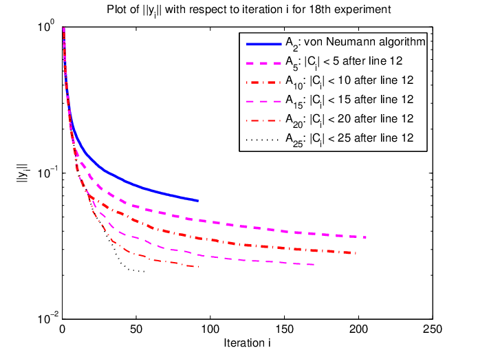
We now explain the bottom diagrams in Figure 5.2. At each iteration $i$ , we calculate

q_{1,i}:=\max_{j\in\{1,\dots,n\}}-a_{j}^{T}y_{i},

just like in solving (2.1). If this quantity is negative, then $A^{T}y_{i}>0$ , and we end. The bottom left diagram shows that, other than a general downward trend, there is no clear pattern in the dependence of $q_{1,i}$ on $i$ . In the bottom right diagram, we calculate

q_{2,i}:=\min_{k\in\{1,\dots,i\}}[\max_{j\in\{1,\dots,n\}}-a_{j}^{T}y_{i}].

We observe that in general, the larger the limit the size of the active set, the faster $q_{2,i}$ (and hence $q_{1,i}$ ) decreases.

5.2. A note on number of iterations and time

We have only discussed the performance of the algorithms we test in terms of iteration counts instead of the time taken. For our experiments so far, we plot the time taken per iteration versus the number of iterations for our implementation of Algorithm 2.1 as well as our implementation of the von Neumann algorithm in Matlab. These are shown in Figure 5.3. The time taken per iteration for Algorithm 2.1 is seen to be between 0.0255 seconds to 0.0290 seconds regardless of the size of $C_{i}$ . The time taken per iteration for the von Neumann algorithm is seen to be between 0.0043 seconds to 0.0047 seconds. Since the running time of the algorithms and the iteration numbers differ only up to a constant factor that is implementation dependent, we shall analyze our algorithms only in terms of the number of iterations. Moreover, it may be possible to improve this ratio in favor of Algorithm 2.1 if the accelerations in Remark 2.12 are carried out, especially when $m$ is large.

5.3. Numerical experiment 2: Aggregation strategies

Table 2 below compares the running times of 353 experiments for the case when (1.1a) is feasible. Rows 1-3 look at the number of iterations it takes to find a certificate vector $y$ , while rows 4-6 look at the norms $\|Ax_{i}\|=\|y_{i}\|$ of the iterates at the $80$ th iteration for the various aggregation methods. For the test on the norms $\|Ax_{i}\|$ , the undecided column denotes the number of times at least one algorithm has found a $y$ such that $A^{T}y>0$ in $80$ iterations. The experiments suggest that the best aggregation method is to aggregate the oldest elements that have not been aggregated. There might be other factors that we have not identified which determine the performance of an aggregation strategy. There could also be better aggregation strategies other than the ones we have tried.

	353 runs for (1.1a) feasible	Best aggregation method
		(1)	(2)	(3)	Ties	Undecided
1	No. iters for $A_{25}$ to find $y$ solving (1.1a)	178	39	102	34	0
2	No. iters for $A_{20}$ to find $y$ solving (1.1a)	173	11	110	59	0
3	No. iters for $A_{15}$ to find $y$ solving (1.1a)	155	10	101	87	0
4	$\\|Ax_{i}\\|$ at $i=80$ for $A_{25}$	62	70	90	0	131
5	$\\|Ax_{i}\\|$ at $i=80$ for $A_{20}$	142	67	96	0	48
6	$\\|Ax_{i}\\|$ at $i=80$ for $A_{15}$	240	37	64	0	12
	126 runs for (1.1b) feasible
7	$\\|Ax_{i}\\|$ at $i=400$ for $A_{15}$	114	10	0	0	2
8	$\\|Ax_{i}\\|$ at $i=400$ for $A_{10}$	121	5	0	0	0
9	$\\|Ax_{i}\\|$ at $i=400$ for $A_{5}$	123	2	1	0	0

Table 2. Experiments on which aggregation strategy is best among those presented in Remark 2.7. The strategies in the three columns are: (1) oldest aggregated, (2) lowest coefficient aggregated, and (3) highest coefficient aggregated, as according to the description in Remark 2.7, which relies on Remark 2.6. For rows 1-6, the 353 experiments are for when (1.1a) is feasible. For rows 7-9, the 126 experiments are for when (1.1b) is feasible. We refer to Subsection 5.3 for more details.

Table 2 also compares the running times of 126 experiments for which (1.1b) is feasible. When (1.1b) is feasible, we want to find iterates $x$ such that $\|Ax\|$ is small. To evaluate the performance of the aggregation strategies, we look at how the norms of the values $\|Ax_{i}\|$ vary with the iteration count $i$ for different strategies. For the test on the norms $\|Ax_{i}\|$ , the undecided column denotes the number of times numerical errors resulting from $\|Ax_{i}\|$ were encountered for at least one algorithm in $400$ iterations. It is quite clear that the strategy of aggregating the oldest point obtained is the best strategy among our experiments.

6. Conclusion

We introduced an improvement of the distance reduction step in the generalized von Neumann algorithm in Algorithm 2.1 by projecting onto the convex hull of a set of points $C_{i}$ using a primal active set QP algorithm. The size of $C_{i}$ , $|C_{i}|$ , can be chosen to be as large as possible, as long as each iteration is manageable. If $|C_{i}|$ is increased, the cost of each iteration increases, but we expect better iterates when (1.2b) is feasible. This is verified by our numerical experiments. When (1.2a) is feasible, we can find a solution to (1.2a) if $|C_{i}|$ is relatively large. But interestingly, if $|C_{i}|$ is small but bigger than $2$ , the performance can be poorer than von Neumann’s algorithm on average.

On the theoretical side, Theorem 3.3 studies the behavior of Algorithm 2.1 when $0\in\mbox{\rm int}(S)$ and the rest of Sections 3 and 4 study the behavior of Algorithm 2.1 when $0\in\partial S$ and $A\in\mathbb{R}^{2\times n}$ . A natural follow up question that better models how Algorithm 2.1 can be used in practice is to study what happens when $|C_{i}|$ is of moderate size. It appears hard to prove such results because there is no easy formula for the projection onto $\mbox{\rm conv}(C_{i})$ when $|C_{i}|>2$ . Remark 4.6 also shows the difficulties for extending our results to the case when $0\in\partial S$ and $A\in\mathbb{R}^{m\times n}$ for $m>2$ . Nevertheless, the results here can give an idea of what can be expected to be true in higher dimensions.

Acknowledgement.

We thank Marina Epelman for organizing Freundfest honoring Robert M. Freund’s 60th birthday, where Javier Peña talked on how Rob Freund’s contributions in the perceptron and von Neumann algorithms influenced his recent work. We also thank Javier Peña for further conversations.

References

[BB96] H.H. Bauschke and J.M. Borwein, On projection algorithms for solving convex feasibility problems, SIAM Rev. 38 (1996), 367–426.
[BCK06] H.H. Bauschke, P.L. Combettes, and S.G. Kruk, Extrapolation algorithm for affine-convex feasibility problems, Numer. Algorithms 41 (2006), 239–274.
[BFV09] A. Belloni, R.M. Freund, and S. Vempala, An efficient rescaled perceptron algorithm for conic systems, Math. Oper. Res. 34 (2009), no. 3, 621–641.
[Blo62] H.D. Block, The perceptron: a model for brain functioning, Rev. Mod. Phys. 34 (1962), 123–135.
[BZ05] J.M. Borwein and Q.J. Zhu, Techniques of variational analysis, Springer, NY, 2005, CMS Books in Mathematics.
[CC01] D. Cheung and F. Cucker, A new condition number for linear programming, Math. Program. 91 (2001), 163–174.
[Cla83] F.H. Clarke, Optimization and nonsmooth analysis, Wiley, Philadelphia, 1983, Republished as a SIAM Classic in Applied Mathematics, 1990.
[Dan92a] G.B. Dantzig, Bracketing to speed convergence illustrated on the von Neumann algorithm for finding a feasible solution to a linear program with a convexity constraint, Technical report SOL 92 (1992), no. 6.
[Dan92b] by same author, An $\epsilon$ -precise feasible solution to a linear program with a convexity constraint in 1/ $\epsilon^{2}$ iterations independent of problem size, Technical Report. Stanford University (1992).
[DV06] J. Dunagan and S. Vempala, A simple polynomial-time rescaling algorithm for solving linear programs, Math. Program. 114 (2006), no. 1, 101–114.
[EF00] M. Epelman and R. M. Freund, Condition number complexity of an elementary algorithm for computing a reliable solution of a conic linear system, Math. Program. 88 (2000), 451–485.
[EF02] by same author, A new condition measure, preconditioners, and relations between different measures of conditioning for conic linear systems, SIAM J. Optim. 12 (2002), no. 3, 627–655.
[ER11] R. Escalante and M. Raydan, Alternating projection methods, SIAM, 2011.
[Fuk82] M. Fukushima, A finitely convergent algorithm for convex inequalities, IEEE Trans. Automat. Control 27 (1982), no. 5, 1126–1127.
[FV99] R.M. Freund and J. Vera, Condition-based complexity of convex optimization in conic linear form via the ellipsoid algorithm, SIAM J. Optim. 10 (1999), 155–176.
[GI83] D. Goldfarb and A. Idnani, A numerically stable dual method for solving strictly convex quadratic programs, Math. Programming 27 (1983), 1–33.
[GP98] U.M. García-Palomares, A superlinearly convergent projection algorithm for solving the convex inequality problem, Oper. Res. Lett. 22 (1998), 97–103.
[GP01] by same author, Superlinear rate of convergence and optimal acceleration schemes in the solution of convex inequality problems, Inherently Parallel Algorithms in Feasibility and Optimization and their Applications (D. Butnariu, Y. Censor, and S. Reich, eds.), Elsevier, 2001, pp. 297–305.
[Mor06] B.S. Mordukhovich, Variational analysis and generalized differentiation I and II, Springer, Berlin, 2006, Grundlehren der mathematischen Wissenschaften, Vols 330 and 331.
[Nes05] Y. Nesterov, Excessive gap technique in nonsmooth convex minimization, SIAM J. Optim. 16 (2005), 235–249.
[Nov62] A.B.J. Novikoff, On convergence proofs on perceptrons, Proceedings of the Symposium on the Mathematical Theory of Automata, vol. XII, 1962, pp. 615–622.
[NW06] J. Nocedal and S.J. Wright, Numerical optimization, 2 ed., Springer, 2006.
[Pan13] C.H.J. Pang, SHDQP: An algorithm for convex set intersection problems based on supporting hyperplanes and dual quadratic programming, ArXiv e-prints (2013).
[Pan14a] by same author, Improved analysis of algorithms based on supporting halfspaces and quadratic programming for the convex intersection and feasibility problems, (preprint) (2014).
[Pan14b] by same author, Set intersection problems: Supporting hyperplanes and quadratic programming, Math. Programming (Online first) (2014).
[Pie84] G. Pierra, Decomposition through formalization in a product space, Math. Programming 28 (1984), 96–115.
[PR00] J. Peña and J. Renegar, Computing approximate solutions for convex conic systems of con- straints, Math. Program. 87 (2000), 351–383.
[Ren95a] J. Renegar, Incorporating condition measures into the complexity theory of linear programming, SIAM J. Optim. 5 (1995), 506–524.
[Ren95b] by same author, Linear programming, complexity theory and elementary functional analysis, Math. Program. 70 (1995), 279–351.
[Roc70] R.T. Rockafellar, Convex analysis, Princeton, 1970.
[Roc79] by same author, Directionally Lipschitzian functions and subdifferential calculus, Proceedings of the London Math. Soc. 3 (1979), 145–154.
[Ros58] F. Rosenblatt, The perceptron: A probabilistic model for information storage and organization in the brain, Psych. Rev. 65 (1958), 386–408.
[Ruj93] P. Ruján, A fast method for calculating the perceptron with maximal stability, J. Physics I France 3 (1993), 277–290.
[RW98] R.T. Rockafellar and R.J.-B. Wets, Variational analysis, Grundlehren der mathematischen Wissenschaften, vol. 317, Springer, Berlin, 1998.
[Sch06] K. Scheinberg, An efficient implementation of an active set method for SVMs, J. Machine Learning Research 7 (2006), 2237–2257.
[SP12] N. Soheili and J. Peña, A smooth perceptron algorithm, SIAM J. Optim. 22 (2012), no. 2, 728–737.
[SP13] by same author, A primal-dual smooth perceptron-von Neumann algorithm, Discrete Geometry and Optimization (K. Bezdek et al., ed.), vol. 69, 2013, pp. 303–320.

Improving the distance reduction step in the von Neumann algorithm

Abstract.

Key words and phrases:

2010 Mathematics Subject Classification

1. Introduction

1.1. Contributions of this paper

1.2. Notation

2. Algorithm

Algorithm 2.1.

Remark 2.2.

Remark 2.3.

Remark 2.4.

Remark 2.5.

2.1. Aggregation strategies

Remark 2.6.

Remark 2.7.

2.2. Primal active set quadratic programming

Algorithm 2.8.

Proposition 2.9.

Remark 2.10.

Remark 2.11.

Remark 2.12.

Algorithm 2.13.

3. Analysis of Algorithm 2.1

Remark 3.1.

Proposition 3.2.

Theorem 3.3.

Proof.

3.1. When 0∈∂S0\in\partial S

Algorithm 3.4.

Theorem 3.5.

Proof.

Theorem 3.6.

Proof.

4. More on Algorithm 3.4

Algorithm 4.1.

Theorem 4.2.

Proof.

Proposition 4.3.

Proof.

Theorem 4.4.

Proof.

Corollary 4.5.

Proof.

Remark 4.6.

5. Numerical experiments

5.1. Numerical experiment 1: Comparison against von Neumann algorithm when AT​y>0A^{T}y>0 feasible

Definition 5.1.

5.2. A note on number of iterations and time

5.3. Numerical experiment 2: Aggregation strategies

6. Conclusion

Acknowledgement.

References

3.1. When $0\in\partial S$

5.1. Numerical experiment 1: Comparison against von Neumann algorithm when $A^{T}y>0$ feasible