跳到论文正文
W Papers独立论文阅读器 arXiv:1408.3070 论文正文 计算阅读时间 · 0%
引用这篇论文根据当前论文元数据生成,正式投稿前建议核对。


License: arXiv.org perpetual non-exclusive license
arXiv:1408.3070v2 [cond-mat.supr-con] 11 Jan 2015

How does the Phase Slip in a Current-Biased Narrow Superconducting Strip?

Yu.N.Ovchinnikov Affiliation: Max-Plank Institute for Physics of Complex Systems, Dresden, D-01187, Germany Affiliation: Landau Institute for Theoretical Physics, RAS, Chernogolovka, Moscow District, 142432 Russia    A.A.Varlamov Affiliation: CNR-SPIN, Viale del Politecnico 1, I-00133, Rome, Italy Affiliation: Materials Science Division, Argonne National Laboratory, 9700 S. Cass Avenue, Argonne, Illinois 60639, USA
August 24, 2026
Abstract

The theory of current transport in a narrow superconducting strip is revisited taking the effect of thermal fluctuations into account. The value of voltage drop across the sample is found as a function of temperature (close to the transition temperature, T−TcT-T_{\mathrm{c}} ≪Tc\ll T_{\mathrm{c}}) and bias current J<JcJ<J_{\mathrm{c}} ( JcJ_{\mathrm{c}} is the critical current calculated in the framework of the BCS approximation, neglecting thermal fluctuations). It is shown that careful analysis of vortices crossing the strip results in considerable increase of the activation energy.

pacs
74.25.Sv, 74.62.-c

I Introduction

The fundamental property of currents flowing dissipationless through superconducting components is the underlying principle for the operation of numerous nano-electronic devices. One component of particular interest is a narrow superconducting strip (NSS), in which thermal and quantum fluctuations can result in a resistive state of the system. Understanding the role of such fluctuations is a problem of great importance. Various models have been proposed to explain the appearance of non-zero resistances in NSSs and its temperature dependence in the region of low temperatures (for a review see Refs. [1, 2]).

The role of thermal fluctuations responsible for energy dissipation, when currents flow through a one-dimensional superconductor was considered for the first time in the paper by Langer and Ambegaokar [3] almost fifty years ago. The publication of this paper has strongly influenced all subsequent studies in this field, becoming part of multiple monographs and handbooks on superconductivity [4, 5, 6].

It is necessary to mention that a “one-dimensional superconductor” is de facto often a narrow strip with finite width LL, much less than the Ginzburg-Landau coherence length ξGL​(T)=π​𝒟/16​T​τ\xi_{\mathrm{GL}}\left(T\right)=\sqrt{\pi\mathcal{D}/16T\tau} (τ=1−T/Tc\tau=1-T/T_{\mathrm{c}} is the reduced temperature and 𝒟\mathcal{D} is the electron diffusion coefficient [7] ). The energy dissipation in this system is related to phase-slip processes, i.e., the process of vortices/flux quanta crossing the strip. It is clear, that such events cannot be realized in the framework of a purely one-dimensional model. Indeed, the solution found in Ref. [3] shows that even when the current density flowing through the one-dimensional superconductor reaches its critical value JcJ_{\mathrm{c}}, the minimal value of the order parameter is (2/3)1/2​ΔBCS,\left(2/3\right)^{1/2}\Delta_{\mathrm{BCS}}, while in order to perform a phase slip event it should become zero at least in one point.

In this work we will resolve the mentioned paradox, describing the true mechanism of phase-slip events in NSS and determining the corresponding value of the activation energy. We will demonstrate that the saddle point solution of the Ginzburg-Landau (GL) equation for the order parameter Δ~\widetilde{\Delta} in presence of a fixed current J,J, possessing at least one vortex, exists only for weak enough currents J<Jc1=η⁡(L/ξGL)​Jc,J<J_{\mathrm{c1}}=\eta\left(L/\xi_{\mathrm{GL}}\right)J_{\mathrm{c}}, (JcJ_{\mathrm{c}} is the critical current of the strip, and η=0.0312\eta=0.0312 is a small number which will be found below). Under the expression “saddle point solution” Δ~(x,y,J,r1,..ri,.)\widetilde{\Delta}\left(x,y,J,r_{1},..r_{i},.\right) we understand the solution of the GL equation, which depends not only on the coordinates x,y,x,y, and current JJ, but also on some set of parameters {𝐫i}\{\mathbf{r}_{i}\} satisfying the extremal conditions for the GL functional ℱs\mathcal{F}_{s}:

∂∂𝐫iℱs[Δ~(x,y,J,𝐫1,..𝐫i),J]=0.\frac{\partial}{\partial\mathbf{r}_{i}}\mathcal{F}_{s}\left[\widetilde{\Delta}\left(x,y,J,\mathbf{r}_{1},..\mathbf{r}_{i}\right),J\right]=0. (1)

In the case under consideration, when one or several vortices penetrate the system through its edge, those parameters can be chosen as the vortex center coordinates (zeros of the order parameter function).

When the current JJ exceeds the value Jc1J_{\mathrm{c1}} the saddle point solutions (1) leading to phase-slip events cease to exist and the scenario described above does not hold anymore. In that case another mechanism comes into play. In order to explain this, let us recall that the minimum of the GL free energy is reached for the ground state, corresponding to a solution with spatially independent modulus |Δgs​(x,y)|=Δ0.|\Delta_{\mathrm{gs}}\left(x,y\right)|=\Delta_{0}. When J<Jc1J<J_{\mathrm{c1}} the saddle point solutions of the GL equations, including vortices, exist with energies higher than the one of the ground state. The transition from the ground-state to the saddle point solution can be imagined as the motion of the order parameter “vector” in Hilbert space, accompanied by the motion of the “points”{𝐫i}\{\mathbf{r}_{i}\} in the finite-dimensional space of those parameters.

As we already said, in the case of “strong currents” Jc1<J<JcJ_{\mathrm{c1}}<J<J_{\mathrm{c}} the saddle point solutions of the GL equations, possessing vortices, do not exist anymore. In this interval the minimal activation energy is reached at some function Δv​(x,y,J,𝐫1)\Delta_{\mathrm{v}}\left(x,y,J,\mathbf{r}_{1}\right) corresponding to the state with a single vortex. We choose such a gauge (i.e. the form of vector potential AA) where the phase of the order parameter is determined by the vortex position only and the boundary conditions at the strip edges. The modulus of Δv​(x,y,J,𝐫1)\Delta_{\mathrm{v}}\left(x,y,J,\mathbf{r}_{1}\right) is an even function of the longitudinal coordinate yy in that case.

In order to determine the order parameter in the state with vortices and subsequently to calculated the corresponding value of free energy, we will use the variational principle with respect to several free parameters in the following. One of them is the distance r1r_{1} from the edge of the strip to the center of a vortex (i.e. the coordinates of the vortex center are x1=−L/2+r1x_{1}=-L/2+r_{1} and y1=0,y_{1}=0, see Fig. 1). We will look for the maximum value r1extr_{1}^{\mathrm{ext}} for which the conditional extremum of the free energy functional (i.e. the extremum at given value of the parameter r1r_{1}) still exists. If the vortex penetrates further into the system, i.e., for r1>r1extr_{1}>r_{1}^{\mathrm{ext}}, such extremum ceases to exist.

Refer to caption
Figure 1: Distribution of the current flowing in the strip in presence of a vortex located in distance r1r_{1} from the edge of the strip.

Let us recall that the order parameter of the current-biased one-dimensional superconducting channel, which corresponds to the saddle point solution of the GL equation does not have zeros at all [3]. When we consider a strip with finite width instead of such a channel a lateral penetration of a vortex is possible. This allows to suppress the modulus of the order parameter to zero at some point allowing a phase-slip event at this location. It is clear that such a deformation of the order parameter on a small scale requires some excess energy. The system partially compensates this energy loss by means of a deformation of the order parameter distribution in relatively large distances from the vortex along the strip with respect to corresponding one-dimensional solution [3]. This deformation is accounted for by means of the variational parameter y0y_{0}. We derive the equations which allow to determine the value of the parameter y0y_{0} maximizing r1r_{1} (i.e. r1extr_{1}^{\mathrm{ext}}) below. It is essential that the value of such penetration depth r1extr_{1}^{\mathrm{ext}} itself does not appear explicitly in the expression for the free energy of the system with the intruded vortex, which is again accounted for by means of y0.y_{0}. It becomes of the order of L\ L for weak enough currents and of the order of the effective coherence length ξG​L​(J)\xi_{GL}(J) (see Eq. (25)) for the strong currents (see Fig. 2).

II Generalities

In order to calculate the value of the activation energy δ​F\delta F for the current-biased NSS we start with the free energy functional ℱs\mathcal{F}_{s} including both GL and the current-field interaction terms (see Ref. [7]):

ℱs\displaystyle\mathcal{F}_{s} =ν∫d3𝐫[−τ|Δ(𝐫)|2+π​𝒟8​T|∂−Δ(𝐫)|2\displaystyle=\nu\int d^{3}\mathbf{r}\left[-\tau|\Delta\left(\mathbf{r}\right)|^{2}+\frac{\pi\mathcal{D}}{8T}|\partial_{-}\Delta\left(\mathbf{r}\right)|^{2}\right. (2)
+7​ζ​(3)16​π2​T2|Δ(𝐫)|4]+1c∫d3𝐫(𝐀(𝐫)−c2​e∇φ)⋅𝐣∞.\displaystyle\left.+\frac{7\zeta\left(3\right)}{16\pi^{2}T^{2}}|\Delta\left(\mathbf{r}\right)|^{4}\right]+\frac{1}{c}\int d^{3}\mathbf{r}\left(\mathbf{A}\left(\mathbf{r}\right)-\frac{c}{2e}\mathbf{\nabla}\varphi\right)\cdot\mathbf{j}_{\infty}.

Here Δ⁡(𝐫)\Delta\left(\mathbf{r}\right) is the order parameter, 𝐀⁡(𝐫)\mathbf{A}\left(\mathbf{r}\right) is vector-potential, ν=m​pF/(2​π2)\nu=mp_{F}/\left(2\pi^{2}\right) is the density of states (pFp_{F} is the electron Fermi momentum), ∂−=∂/∂𝐫−2ie𝐀/c\partial_{-}=\partial/\partial\mathbf{r-}2ie\mathbf{A/}c, ζ⁡(x)\zeta\left(x\right) is the Riemann zeta-function, j∞j_{\infty} =J/S,=J/S, SS is the cross-section of the stripe, cc is the speed of light, φ\varphi is the phase of the order parameter. We use the system of units where kB=1k_{\mathrm{B}}=1 and ℏ=1.\hbar=1.This functional allows to write down the equations both for order parameter and vector-potential coordinate dependencies.

Close to zero current value. Let us start with the simplest case of zero current, j∞=0.j_{\infty}=0. In this case an infinite number of saddle point solutions exist. If the saddle point solution has only one zero corresponding to a single vortex state, symmetry considerations show that the center of this vortex is located at the central line of the strip (see Fig. 3). Choosing the latter as the center of coordinates one can find that the phase and modulus of the order parameter are determined as:

[∂φ⁡(x,y)∂𝐫]2=π2L2​1sin2⁡(π​x/L)+sinh2⁡(π​y/L),\left[\frac{\partial\varphi\left(x,y\right)}{\partial\mathbf{r}}\right]^{2}=\frac{\pi^{2}}{L^{2}}\frac{1}{\sin^{2}\left(\pi x/L\right)+\sinh^{2}\left(\pi y/L\right)}, (3)
|Δ⁡(x,y,y0)|=π​Δ0L​cosh⁡π​yL​1(∂φ/∂𝐫)2​tanh⁡y2+y022​ξGL,\left|\Delta(x,y,y_{0})\right|=\frac{\pi\Delta_{0}}{L\cosh\frac{\pi y}{L}}\frac{1}{\sqrt{\left(\partial\varphi/\partial\mathbf{r}\right)^{2}}}\tanh\frac{\sqrt{y^{2}+y_{0}^{2}}}{2\xi_{\mathrm{GL}}},\quad (4)

where LL is the width of the strip and y0y_{0} is the free parameter discussed at the end of the introduction (see also Fig. 2). The phase of the order parameter φ\varphi is the solution of the two dimensional Laplace equation Δ​φ=0\Delta\varphi=0 with boundary conditions ∂φ/∂x|x=±L/2=0.\left.\partial\varphi/\partial x\right|_{x=\pm L/2}=0. The expression (4), obtained by means of the variational procedure, coincides with the corresponding solution of the GL equation in the limit |y|≫L|y|\gg L.

Refer to caption
Figure 2: Distribution of the modulus of the order parameter in the strip with flowing current disturbed in the presence of a vortex: a) transversal distribution at y=0y=0; b) longitudinal distribution at x=0x=0.

Substitution of Eqs. (3) and (4) to Eq. (2) gives the value of the activation energy versus y0:y_{0}:

δ​F(1)​(y0)=4​ν​Δ02​τ​S​ξGL​{23−π​y08​ξGL+L4​π​ξGL​[8​π2​(y0/L)2+4​ζ​(2)−16+π2​y022​L2​I0​(π​y0L)]},\delta F^{\left(1\right)}\left(y_{0}\right)\!=\!4\nu\Delta_{0}^{2}\tau S\xi_{\mathrm{GL}}\left\{\frac{2}{3}\!-\!\frac{\pi y_{0}}{8\xi_{\mathrm{GL}}}+\!\frac{L}{4\pi\xi_{\mathrm{GL}}}\left[\frac{8\pi^{2}\left(y_{0}/L\right)^{2}+4\zeta\left(2\right)-1}{6}\!\!+\!\frac{\pi^{2}y_{0}^{2}}{2L^{2}}I_{0}\left(\!\frac{\pi y_{0}}{L}\right)\right]\right\}, (5)

with

I0​(α)=∫0∞d​xcosh2⁡x​1x2+α2.I_{0}\left(\!\alpha\right)=\int_{0}^{\infty}\frac{dx}{\cosh^{2}x}\frac{1}{x^{2}+\alpha^{2}}.

The details of derivation of Eq. (5) are given in Appendix A.

Refer to caption
Figure 3: Positions of the zeros of the saddle point solutions with one (a), two (b), etc, vortices. Here by means of {+,−}\{+,-\} are denoted the vorticities (phase factor changes by ±2​π\pm 2\pi for anticlock/clockwise circulation of the order parameter zeros).

Minimization of Eq. (5) over y0y_{0} gives the value y0=0.47​L/π;y_{0}=0.47L/\pi; the corresponding value for the one-vortex configuration activation energy is

δ​F(1)=4​ν​Δ02​τ​S​ξGL​(23+0.058​LξGL).\delta F^{\left(1\right)}=4\nu\Delta_{0}^{2}\tau S\xi_{\mathrm{GL}}\left(\frac{2}{3}+0.058\frac{L}{\xi_{\mathrm{GL}}}\right). (6)

An analogous consideration of the two vortices configuration gives for δ​F(2)\delta F^{\left(2\right)} an answer similar to Eq. (6) with the second term in brackets being twice smaller (see Appendix A). Further increase of the number of zeros in the order parameter results in the decrease of the second term in δ​F(n)\delta F^{\left(n\right)} by the factor nn with respect to δ​F(1)\delta F^{\left(1\right)}. In the limit n→∞n\rightarrow\infty the latter reaches the value

δ​F(∞)=8​ν​Δ02​τ​S​ξGL/3\delta F^{\left(\infty\right)}=8\nu\Delta_{0}^{2}\tau S\xi_{\mathrm{GL}}/3 (7)

first obtained in Ref. [3] in the frameworks of the one-dimensional model.

The flow of any finite current through the strip results in the finiteness of the number of the saddle point solutions. This number rapidly decreases with the current growth and already at so small current as Jc1=η⁡(L/ξG​L)​JcJ_{\mathrm{c1}}=\eta\left(L/\xi_{GL}\right)J_{\mathrm{c}} the only saddle point solution with one vortex remains. At higher currents the saddle point solutions do not exist more, the critical points appear instead of them.

One can see that at zero current, the solution of the GL equation found in Ref. [3] actually is the limiting one for the multiple-vortex solutions obtained above. As a result we can state that the point J=0J=0 is a singular point in the current dependence of the activation energy. Therefore the dependence of δ​F(∞)​(J)\delta F^{\left(\infty\right)}(J), obtained in Ref. [3] for small currents as the linear, in fact turns out to be substantially more complicated. It is worth to mention that the multiplicity of saddle point solutions in the domain of weak currents results in an increase of the possibilities of the phase-slip events, i.e., to a noticeable increase of the pre-exponential factor.

III “Weak” currents

Now we consider the most simple one-vortex state in the region of weak currents J≤Jc​1.J\leq J_{c1}. The vortex, corresponding to the saddle point solution, now slightly shifts with respect to the central axis of the strip. Denoting the distance between the axis (x=0x=0) and vortex center as δ\delta ( δ=L/2−r1\delta=L/2-r_{1}), we look for the solution of the Ginzburg-Landau equation in the form

|Δ|=Δ0​(Γ)​Z1/2​(y2+y02)​Φ​(x,y,δ),\left|\Delta\right|=\Delta_{0}\left(\Gamma\right)Z^{1/2}\left(\sqrt{y^{2}+y_{0}^{2}}\right)\Phi\left(x,y,\delta\right), (8)

with the functions

Φ2​(x,y,δ)=sinh2⁡(π​y/L)+sin2⁡(π​x/L)+sin2⁡(π​δ/L)−2​cosh⁡(π​y/L)​sin⁡(π​x/L)​sin⁡(π​δ/L)cosh2⁡(π​y/L)\Phi^{2}\left(x,y,\delta\right)=\frac{\sinh^{2}\left(\pi y/L\right)+\sin^{2}\left(\pi x/L\right)+\sin^{2}\left(\pi\delta/L\right)-2\cosh\left(\pi y/L\right)\sin\left(\pi x/L\right)\sin\left(\pi\delta/L\right)}{\cosh^{2}\left(\pi y/L\right)} (9)

and

Z⁡(y,Γ)=1−3​ℒ−2ℒ​[cosh⁡(y​3​ℒ−22​ξGL)]−2.Z\left(y,\Gamma\right)=1-\frac{3\mathcal{L}-2}{\mathcal{L}}\left[\cosh\left(\frac{y\sqrt{3\mathcal{L}-2}}{2\xi_{\mathrm{GL}}}\right)\right]^{-2}. (10)

Here Γ=J/Jc,\Gamma=J/J_{c}, while Δ0​(Γ)\Delta_{0}\left(\Gamma\right) is the order parameter of the homogeneous ground state of the NSS carrying on the current JJ, i.e. the asymptotic form of our Δ⁡(x,y,Γ,y0,​δ)\Delta\left(x,y,\Gamma,y_{0,}\delta\right) far from the vortex, at y→±∞y\rightarrow\pm\infty. The latter can be related to the BCS value Δ00​(τ)=[8​π2​T2​τ/(7​ζ​(3))]1/2\Delta_{00}{}\left(\tau\right)=\left[8\pi^{2}T^{2}\tau/\left(7\zeta\left(3\right)\right)\right]^{1/2} of the order parameter in the absence of current by means of the relation

Δ02​(Γ)=Δ002​ℒ​(Γ).\Delta_{0}^{2}{}\left(\Gamma\right)=\Delta_{00}^{2}\mathcal{L}\left(\Gamma\right). (11)

The choice of the two former multipliers in the anzatz (8) is based on the Langer-Ambegaokar solution of the GL equation for current biased one-dimensional channel distorted by the vortex presence (and accounting for its evenness in yy). The latter multiplier (see Eq. (9)) accounts for the appearing in the case under consideration asymmetry of the order parameter dependence on the transversal coordinate and in the case of δ=0\delta=0 it leads to the coincidence of Eq. (8) and Eqs. (4)-(3). Substitution of the anzatz (8), (9), and (10) to the GL equations gives the explicit value for ℒ⁡(Γ):\mathcal{L}\left(\Gamma\right):

ℒ⁡(Γ)=13+23​sin⁡[π6+23​arcsin⁡1−Γ2].\mathcal{L}\left(\Gamma\right)=\frac{1}{3}+\frac{2}{3}\sin\left[\frac{\pi}{6}+\frac{2}{3}\arcsin\sqrt{1-\Gamma^{2}}\right]. (12)

The quantity y0∼L,y_{0}\sim L, hence for |y|≫L\left|y\right|\gg L the modulus of the order parameter |Δ|\left|\Delta\right| (see Eq. (8)) should obey the exact GL equations with the corresponding boundary conditions at x=±L/2.x=\pm L/2. The function Φ\Phi is related to the order parameter phase φ\varphi which satisfies the equation

(∂φ⁡(x,y)∂𝐫)2=(πL)2​cos2⁡π​δLcosh2⁡(π​yL)​Φ2​(x,y,δ).\left(\frac{\partial\varphi\left(x,y\right)}{\partial\mathbf{r}}\right)^{2}=\left(\frac{\pi}{L}\right)^{2}\frac{\cos^{2}\frac{\pi\delta}{L}}{\cosh^{2}\left(\frac{\pi y}{L}\right)\Phi^{2}\left(x,y,\delta\right)}. (13)

Substitution of the Eqs. (8), (9), and (13) into Eq. (2) leads to the expression for free energy

δ​Fδ​(y0)\displaystyle\delta F_{\delta}\left(y_{0}\right) =4νΔ02τSξGL{23−π​y08​ξGL−16​π​ξGL​Γ227​L(π4​a+L8​y0+I1(a))+L4​π​ξGL[4​a23+23ζ(2)−16+a22I0(a)]\displaystyle=4\nu\Delta_{0}^{2}\tau S\xi_{\mathrm{GL}}\left\{\frac{2}{3}-\frac{\pi y_{0}}{8\xi_{\mathrm{GL}}}-\frac{16\pi\xi_{\mathrm{GL}}\Gamma^{2}}{27L}\left(\frac{\pi}{4a}+\frac{L}{8y_{0}}+I_{1}\left(a\right)\right)+\frac{L}{4\pi\xi_{\mathrm{GL}}}\left[\frac{4a^{2}}{3}+\frac{2}{3}\zeta\left(2\right)-\frac{1}{6}+\frac{a^{2}}{2}I_{0}\left(\!a\right)\right]\right.
+π​Γ323sin(πδ/L)−L4​π​ξGL[2​a23+13ζ(2)+a2I0(a)]sin2(πδ/L)},\displaystyle\left.+\frac{\pi\Gamma}{3}\sqrt{\frac{2}{3}}\sin\left(\pi\delta/L\right)-\frac{L}{4\pi\xi_{\mathrm{GL}}}\left[\frac{2a^{2}}{3}+\frac{1}{3}\zeta\left(2\right)+a^{2}I_{0}\left(a\right)\right]\sin^{2}\left(\pi\delta/L\right)\right\}, (14)

where

a2=π2​y02L2+32​π2​Γ227​L2​ξGL2a^{2}=\frac{\pi^{2}y_{0}^{2}}{L^{2}}+\frac{32\pi^{2}\Gamma^{2}}{27L^{2}}\xi_{\mathrm{GL}}^{2}

and

I1​(a)=∫0∞d​xcosh⁡x​1x2+4​a2.I_{1}\left(\!a\right)=\int_{0}^{\infty}\frac{dx}{\cosh x}\frac{1}{x^{2}+4a^{2}}.

The details of transition from Eq. (2) to Eq. (14) are presented in the Appendix A.

Let us recall, that the quantities {y0,δ}\left\{y_{0},\delta\right\} still remain indefinite: their values one can determine from the conditions of the GL functional δ​Fδ​(y0)\delta F_{\delta}\left(y_{0}\right) extremum:

∂δ​Fδ​(y0)∂y0=0,\frac{\partial\delta F_{\delta}\left(y_{0}\right)}{\partial y_{0}}=0,\; (15)
∂δ​Fδ​(y0)∂δ=0\frac{\partial\delta F_{\delta}\left(y_{0}\right)}{\partial\delta}=0 (16)

In result of solution of Eq. (16) the value δ\delta can be presented as the function of Γ:\Gamma:

sin⁡π​δL=(23)3/2​π2​ξGL​ΓL⁡[2​a2/3+ζ⁡(2)/3+a2​I0​(a)].\sin\frac{\pi\delta}{L}=\left(\frac{2}{3}\right)^{3/2}\frac{\pi^{2}\xi_{\mathrm{GL}}\Gamma}{L\left[2a^{2}/3+\zeta\left(2\right)/3+a^{2}I_{0}\left(a\right)\right]}. (17)

What concerns the value y0y_{0} it is determined by Eqs. (15) and (17). Corresponding equation is very cumbersome and we do not present it here. Important, that it has the solution only in the very narrow currents interval

Γ2≤Γc​12=0.009​L2ξGL2.\Gamma^{2}\leq\Gamma_{c1}^{2}=0.009\frac{L^{2}}{\xi_{\mathrm{GL}}^{2}}.

Finally, the value of the free energy δ​Fδ\delta F_{\delta} in the critical point J=Jc​1J=J_{c1} is

δ​Fδ​(τ,Jc​1)=4​ν​Δ02​(Γ)​τ​S​ξGL​(23+0.054​LξGL).\delta F_{\delta}\left(\tau,J_{c1}\right)=\!4\nu\Delta_{0}^{2}\left(\Gamma\right)\tau S\xi_{\mathrm{GL}}\left(\frac{2}{3}+0.054\frac{L}{\xi_{\mathrm{GL}}}\right). (18)

Comparing the Eqs. (18) and (6) one can see that the state with J=Jc​1J=J_{c1}, when the only saddle point solution with one vortex remains, energetically differs from that one with J=0J=0 by very small quantity 0.004​(LξGL)​4​ν​Δ02​(Γ)​τ​S​ξGL0.004\left(\frac{L}{\xi_{\mathrm{GL}}}\right)4\nu\Delta_{0}^{2}\left(\Gamma\right)\tau S\xi_{\mathrm{GL}}.

IV “Strong” currents

Let us pass to discussion of the mechanism of energy dissipation in the wide range of currents Jc​1≪J<Jc,J_{c1}\ll J<J_{c}, when the GL equations do not have more any saddle point solution. Let us suppose that through the edge of the strip penetrates a single vortex and assume that its center is located at some small distance r1​(r1≪L)r_{1}(r_{1}\ll L) from the edge, i.e. the vortex center coordinates are: (−L/2+r1,0)\left(-L/2+r_{1},0\right). Our goal is to obtain the maximal possible value of the “penetration length” r1r_{1} at which the requirement of existence of the conditional extremum of the functional (2) is still satisfied. In order to do this we look for the phase and the modulus of the order parameter in the form containing three free parameters: r1,y0,γr_{1},y_{0},\gamma

(∂φ⁡(x,y,r1)∂𝐫)2=(πL)2​sin2⁡π​r1Lcosh4⁡(π​y2​L)​[Q⁡(x,y)]−1,\left(\frac{\partial\varphi\left(x,y,r_{1}\right)}{\partial\mathbf{r}}\right)^{2}=\left(\frac{\pi}{L}\right)^{2}\frac{\sin^{2}\frac{\pi r_{1}}{L}}{\cosh^{4}\left(\frac{\pi y}{2L}\right)}\left[Q(x,y)\right]^{-1}, (19)

and

|Δ⁡(x,y,r1,y0,γ)|=Δ0​(Γ)​ln⁡[+γ​L2r12​Q1/2​(x,y)]ln⁡(2​γ​L2r12+1)​Z12​(Γ,y+y0)\left|\Delta\left(x,y,r_{1},y_{0},\gamma\right)\right|\!=\!\Delta_{0}\left(\Gamma\right)\frac{\ln\left[1\!+\!\frac{\gamma L^{2}}{r_{1}^{2}}Q^{1/2}(x,y)\right]}{\ln\left(\frac{2\gamma L^{2}}{r_{1}^{2}}+1\right)}\!Z^{\frac{1}{2}}\!\left(\Gamma,\!y\!+\!y_{0}\right) (20)

The function

Q⁡(x,y,r1)\displaystyle Q(x,y,r_{1}) ={4sinh2(π​y2​L)[cosh2π​y2​L+cosπ​r1Lsinπ​xL]\displaystyle=\left\{4\sinh^{2}\left(\frac{\pi y}{2L}\right)\left[\cosh^{2}\frac{\pi y}{2L}+\cos\frac{\pi r_{1}}{L}\sin\frac{\pi x}{L}\right]\right.
+[sinπ​xL+cosπ​r1L]2}[cosh(π​y2​L)]−4,\displaystyle\left.+\left[\sin\frac{\pi x}{L}+\cos\frac{\pi r_{1}}{L}\right]^{2}\right\}\left[\cosh\left(\frac{\pi y}{2L}\right)\right]^{-4}, (21)

is the result of direct calculation of the phase φ\varphi in the one-vortex state of the strip (see Eq. (19)). The function |Δ⁡(x,y)|\left|\Delta\left(x,y\right)\right| approaches to the solution of the GL equation in the range |y|≫L\left|y\right|\gg L. Both Eqs. (19) and (20) satisfy the boundary conditions for the order parameter and its derivatives at the edge of the stripe and at infinity. What concerns the variational parameter γ\gamma it can be found from the condition

∂δ​F​(r1,y0,γ)∂γ=0.\frac{\partial\delta F\left(r_{1},y_{0},\gamma\right)}{\partial\gamma}=0. (22)

It determines the shape of the order parameter and, correspondingly, the contribution to the free energy from the domain close to the vortex |y|≲L|y|\lesssim L. Its introduction allows to improve the variational approximation in this region. Corresponding expression turns to be of the order of 1 and does not appear explicitly in the final expression for the free energy, it is why we do not present it here.

The current conservation law leads to the next expression for the essential part of the vector potential 𝐀\mathbf{A}

Ay(0)​(y)=A∞​Δ02​(Γ)⟨|Δ⁡(x,y)|2⟩x,A_{y}^{\left(0\right)}\left(y\right)=\frac{A_{\infty}\Delta_{0}^{2}{}\left(\Gamma\right)}{\left\langle|\Delta\left(x,y\right)|^{2}\right\rangle_{x}{}}, (23)

where ⟨….⟩x\left\langle....\right\rangle_{x} means the averaging over the transverse coordinate. The value of the vector potential at infinity A∞A_{\infty} is determined by the current density:

JS=−π​ν​e2​𝒟T​Δ02​(Γ)​A∞.\frac{J}{S}=-\frac{\pi\nu e^{2}\mathcal{D}}{T}\Delta_{0}^{2}{}\left(\Gamma\right)A_{\infty}. (24)

Replacing the expressions (19) , (20) , and (23) to the GL functional (2) and calculating the integral one can find the value of excess free energy δ​Fs\delta F_{s} of the strip with the penetrated vortex with respect to its the ground state with the fixed current. The requirement of existence of the conditional extremum determines the value y0:y_{0}:

y0​(Γ)=2​ξGL​Yℒ3​ℒ−2,y_{0}\left(\Gamma\right)=\frac{2\xi_{\mathrm{GL}}Y_{\mathcal{L}}}{\sqrt{3\mathcal{L}-2}}, (25)
tanh⁡Yℒ​(Γ)=2​[(1−ℒ)4−3​ℒ+ℒ⁡(16−15​ℒ)]1/2.\tanh Y_{\mathcal{L}}\left(\Gamma\right)=2\left[\frac{\left(1-\mathcal{L}\right)}{4-3\mathcal{L}+\sqrt{\mathcal{L}\left(16-15\mathcal{L}\right)}}\right]^{1/2}.\quad

The main steps of this calculus are presented in the Appendix B. The obtained results allow us to write down the expression for the activation energy in the whole region of “strong currents” Jc​1≪J<JcJ_{c1}\ll J<J_{c} :

δ​F​(τ,J)\displaystyle\delta F\left(\tau,J\right) =4νΔ02(Γ)τSξGL(3​ℒ−2){1−tanh⁡Yℒ6​ℒ[4+(3ℒ−2)tanhYℒ(1+tanhYℒ)]\displaystyle=4\nu\Delta_{0}^{2}\left(\Gamma\right)\tau S\xi_{\mathrm{GL}}\sqrt{\left(3\mathcal{L}-2\right)}\left\{\frac{1-\tanh Y_{\mathcal{L}}}{6\mathcal{L}}\left[4+\left(3\mathcal{L}-2\right)\tanh Y_{\mathcal{L}}\left(1+\tanh Y_{\mathcal{L}}\right)\right]\right.
−2​(1−ℒ)3​ℒ−2[arctan3​ℒ−22​(1−ℒ)−arctan(3​ℒ−22​(1−ℒ)tanhYℒ)]}.\displaystyle-\left.\sqrt{\frac{2\left(1-\mathcal{L}\right)}{3\mathcal{L}-2}}\left[\arctan\sqrt{\frac{3\mathcal{L}-2}{2\left(1-\mathcal{L}\right)}}-\arctan\left(\sqrt{\frac{3\mathcal{L}-2}{2\left(1-\mathcal{L}\right)}}\tanh Y_{\mathcal{L}}\right)\right]\right\}. (26)

It is seen that the difference between Eq. (26) and the expression for the activation energy of the one-dimensional superconducting channel carrying current JJ (the main result of Ref. [3]) consists of the contribution occurring due to the nonzero value of the parameter Yℒ,Y_{\mathcal{L}}, i.e. due to existence of the conditional extremum of the free energy functional at the distance y0≠0y_{0}\neq 0. Let us stress that the activation energy δ​F\delta F depends on the geometry of a sample, which here is assumed as a strip. The increase of the energy barrier in the Arrenius law with respect to the result of Ref. [3] is related to the necessity of the vortex penetration in a sample at the moment of the phase slip event.

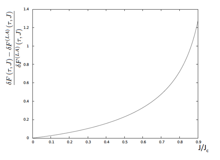
The expression for activation energy δ​F(L​A)​(τ,J)\delta F^{\left(LA\right)}\left(\tau,J\right) of the one-dimensional superconducting channel found in Ref. [3] can be easily reproduced from Eq. (26) just putting Yℒ=0Y_{\mathcal{L}}=0 (what follows from Eq. (25)). One can compare the result of our careful consideration of the vortex penetration mechanisms (26) with the latter:

δ​F​(τ,J)−δ​F(L​A)​(τ,J)δ​F(L​A)​(τ,J)=[3​ℒ−26​ℒtanh⁡Yℒcosh2⁡Yℒ−2tanh⁡Yℒ3​ℒ+2​(1−ℒ)3​ℒ−2arctan(3​ℒ−22​(1−ℒ)tanhYℒ)][23​ℒ−2​(1−ℒ)3​ℒ−2​arctan⁡3​ℒ−22​(1−ℒ)].\frac{\delta F\left(\tau,J\right)-\delta F^{\left(LA\right)}\left(\tau,J\right)}{\delta F^{\left(LA\right)}\left(\tau,J\right)}=\frac{\left[\frac{3\mathcal{L}-2}{6\mathcal{L}}\frac{\tanh Y_{\mathcal{L}}}{\cosh^{2}Y_{\mathcal{L}}}-2\frac{\tanh Y_{\mathcal{L}}}{3\mathcal{L}}+\sqrt{\frac{2\left(1-\mathcal{L}\right)}{3\mathcal{L}-2}}\arctan\left(\sqrt{\frac{3\mathcal{L}-2}{2\left(1-\mathcal{L}\right)}}\tanh Y_{\mathcal{L}}\right)\right]}{\left[\frac{2}{3\mathcal{L}}-\sqrt{\frac{2\left(1-\mathcal{L}\right)}{3\mathcal{L}-2}}\arctan\sqrt{\frac{3\mathcal{L}-2}{2\left(1-\mathcal{L}\right)}}\right]}. (27)

.

For the currents larger than Jc​1J_{c1} but still much smaller than JcJ_{c} the saddle point solutions of GL equations considered in Ref. [3] do not exist more. Nevertheless one can see that the difference between the free energy of the conditional extremum and that one calculated by Langer and Ambegaokar (see Eq. (27)) turns to be proportional only to (J/Jc)2,\left(J/J_{c}\right)^{2}, i.e. the result of Ref. [3] remains valid. The situation considerably changes when the current approaches its critical value, J→JcJ\rightarrow J_{c}(Γ→1\Gamma\rightarrow 1). Here tanh⁡Yℒ→1/3;cosh2⁡Yℒ→3/2;1+2−1​cosh−2⁡Yℒ−L​tanh2⁡Yℒ/[2​(1−ℒ)]→1;3​L−2→23/2​1−Γ/3\tanh Y_{\mathcal{L}}\rightarrow 1/\sqrt{3};\cosh^{2}Y_{\mathcal{L}}\rightarrow 3/2;1+2^{-1}\cosh^{-2}Y_{\mathcal{L}}-L\tanh^{2}Y_{\mathcal{L}}/\left[2\left(1-\mathcal{L}\right)\right]\rightarrow 1;3L-2\rightarrow 2^{3/2}\sqrt{1-\Gamma}/\sqrt{3}, and

δF(L​A)(τ,Γ→1)=41523ντΔ002(τ)SξGL(1−Γ2)5/4,\delta F^{\left(LA\right)}\left(\tau,\Gamma\rightarrow 1\right)=\frac{4}{15}\sqrt{\frac{2}{\sqrt{3}}}\nu\tau\Delta_{00}^{2}\left(\tau\right)S\xi_{\mathrm{GL}}\left(1-\Gamma^{2}\right)^{5/4}, (28)

while

δF(τ,Γ→1)=23/239/4ντΔ002(τ)SξGL(1−Γ2)3/4.\delta F\left(\tau,\Gamma\rightarrow 1\right)=\frac{2^{3/2}}{3^{9/4}}\nu\tau\Delta_{00}^{2}\left(\tau\right)S\xi_{\mathrm{GL}}\left(1-\Gamma^{2}\right)^{3/4}. (29)

The relative difference of the free energies Eq. (27) in this case diverges:

δ​F​(τ,J)−δ​F(L​A)​(τ,J)δ​F(L​A)​(τ,J)|J→Jc=5​Jc6​Jc2−J2,\left.\frac{\delta F\left(\tau,J\right)-\delta F^{\left(LA\right)}\left(\tau,J\right)}{\delta F^{\left(LA\right)}\left(\tau,J\right)}\right|_{J\rightarrow J_{c}}=\frac{5J_{c}}{6\sqrt{J_{c}^{2}-J^{2}}}, (30)

i.e. the height of the barrier in Arrenius law turns out to be parametrically larger than predicted in Ref. [3]. The behavior of Eq. (27) as the function of Γ\Gamma in the interval [0,0.9]\left[0,0.9\right] is presented in Fig. 4.

Refer to caption
Figure 4: Excess activation energy related to the account for the true mechanism of the vortices penetration in the strip as the function of flowing current.

V Pre-exponential factor

In order to obtain the exact value of the pre-exponential factor Ω\Omega for phase slip events one should have in possession the expression for the effective action of superconducting strip containing vortices. In the Ref. [8] was proposed a general procedure which, in the regime of thermal fluctuations, is reduced to solution of the spectral problem for linear operator corresponding to the action at its saddle point. The difficulty of the problem under consideration consists in the fact that nor microscopic action operator is known nor saddle point (for currents OPENJc​1<J)J_{c1}<J) exists. Nevertheless, the knowledge of action would allow one to get the precise value of Ω\ \Omega at least for weak currents J<Jc​1,J<J_{c1}, while for strong currents one could believe that change of the saddle point to a singular point would not strongly effect on the value of pre-exponential factor. In light of the above said the evaluations of Ω\Omega in both papers [3, 9] seem doubtful: use of the time-dependent GL equation below TcT_{\mathrm{c}} as today is well known cannot be justified, unless in gapless regime[10].

The main contribution to the average time between two subsequent phase-slip events is related to the existence of the “zero-mode” (see Ref. [9, 8]). In the case under consideration the size of the vortex is determined by the transversal size LL of the strip. The vortices which slip on the distances larger than LL can be considered as independent. It is why the main factor determining the pre-exponential one is the ratio of the transversal size LL to the strip length 𝔏\mathfrak{L}: L/𝔏.L/\mathfrak{L.} Another coefficient which forms the pre-exponential factor is the characteristic “crossing time” Δ​tcross=L/vcross\Delta t_{\mathrm{cross}}=L/v_{\mathrm{cross}} of the strip by the vortex, moving with the velocity [12]:

vcross=c​J​τ4​S​Hc​2​σn,v_{\mathrm{cross}}=\frac{cJ\sqrt{\tau}}{4SH_{c2}\sigma_{n}}, (31)

where σn\sigma_{n} is the conductivity of the strip in its normal phase. Finally, accounting for Arrenius factor, one finds the characteristic time Δ​t\Delta t between two phase slipping events

Δ​t=L𝔏​(Lvcross)​exp⁡(δ​FkB​T).\Delta t=\frac{L}{\mathfrak{L}}\left(\frac{L}{v_{\mathrm{cross}}}\right)\exp\left(\frac{\delta F}{k_{\mathrm{B}}T}\right). (32)

The average voltage VV at the strip is related to the average time interval Δ​t\Delta t between the voltage jumps by the Josephson relation[11]: V=π​ℏ/(e​Δ​t).V=\pi\hbar/\left(e\Delta t\right). Corresponding resistance of the strip is

RR0=π​ℏ​c​τ4​e​Hc​2​L2​exp⁡[−δ​F​(τ,Γ)kB​T],\frac{R}{R_{0}}=\frac{\pi\hbar c\sqrt{\tau}}{4eH_{c2}L^{2}}\exp\left[-\frac{\delta F\left(\tau,\Gamma\right)}{k_{\mathrm{B}}T}\right], (33)

where R0=𝔏/(σn​S)R_{0}=\mathfrak{L}/\left(\sigma_{n}S\right) is the normal resistance of the strip. It is necessary to mention that the used above approximation of the independent phase slips is valid only (according to Eq. (32) ) when δ​F≳kB​T.\delta F\gtrsim k_{\mathrm{B}}T.

VI Conclusions

We have demonstrated that considering only the longitudinal spatial dependence of the order parameter in narrow superconducting strips carrying finite current (see Ref. [3]) is not sufficient to describe the properties of its resistive state correctly. Taking the transversal coordinate into account when calculating the saddle point solutions of the GL equation turns out to be essential. Namely, the value of activation energy in the Arrenius law for the resistance of a narrow superconducting channel differs already for relatively weak currents from the value obtained by simply using the difference of the free energy of such a saddle point and the ground state energy. The mechanism for phase-slip events turns out to be much more sophisticated then the one described in Ref. [3].

Already at weak currents (J<Jc1J<J_{\mathrm{c1}}) a sequence of the saddle points appears, which is characterized by the number nn of zeros of the order parameter along the transverse coordinate. The energy of such state equals to that one found by Langer and Ambegaokar [3] only in the limit n→∞,n\rightarrow\infty, when the system carries no current. One could say that the state of the strip in the current-free case is singular. The number nn of saddle points rapidly decreases with the growth of the current. It reaches n=1n=1 when the current has the value Jc1=0.0312​(L/ξ)​JcJ_{\mathrm{c1}}=0.0312\left(L/\xi\right)J_{\mathrm{c}}: at this point only a stationary state remains.

When J>Jc1J>J_{\mathrm{c1}}, stationary solutions of the GL equations with fixed current and a vortex in the strip do not exist. Instead one needs to look for a critical point, corresponding to the existence of a specific conditional extremum of the GL functional. These conditions are: the current, JJ, is fixed and the distance between the vortex center and the strip edge is maximal. The energy of such a state turns out to be larger than the activation energy δ​F(L​A)​(τ,J)\delta F^{\left(LA\right)}\left(\tau,J\right) obtained in Ref. [3]. The normalized difference (30) increases with growth of the current and when the latter approaches to the critical value JcJ_{c} the former diverges (see Fig. 4).

Experimentally, the discrepancy between the theoretical prediction of Ref. [3] and the mechanism proposed here can be detected by analyzing the current dependence of the resistance close to Jc.J_{\mathrm{c}}. The predicted dependence of log⁡R⁡(I)\log R(I) with exponent 5/45/4 in Ref. [3], should transform into a weaker one with exponent 3/43/4 in the region J→JcJ\rightarrow J_{c}. Some experimental papers indicated an unexpected decrease of the resistance in the regime of strong currents (see Ref. [4, 13, 14]). This long standing enigma can potentially be resoled by the above analysis. A recent numerical study narrow superconducting channels using the time-dependent GL equation in the strong current regime also indicated that the critical exponent of the activation energy is of the order of 0.7 for the widths L∼ξG​LL\sim\xi_{GL} (see Ref. [15]).

Acknowledgements.
The authors acknowledge financial support of the FP7-IRSES program, grant N 236947 “SIMTECH”. A.V. was partially supported by the U.S. Department of Energy, Office of Science, Office of Advanced Scientific Computing Research and Materials Sciences and Engineering Division, Scientific Discovery through Advanced Computing (SciDAC) program. A.V. is grateful to I. Aronson, A. Bezryadin and A. Glatz for valuable discussions.

Appendix A

In the process of derivation of Eq. (5) we used the following integrals:

1L∫−L/2L/2d​xsin2⁡π​xL+sinh2⁡π​yL=2sinh⁡(2​π​yL),\frac{1}{L}\int_{-L/2}^{L/2}\frac{dx}{\sin^{2}\frac{\pi x}{L}+\!\sinh^{2}\frac{\pi y}{L}}\!=\!\frac{2}{\sinh\left(\frac{2\pi y}{L}\right)}, (34)
1L∫−L/2L/2sin2⁡(π​x/L)​d​xsin2⁡π​xL+sinh2⁡π​yL=exp⁡(−π​yL)cosh⁡π​yL,\frac{1}{L}\int_{-L/2}^{L/2}\frac{\sin^{2}\left(\pi x/L\right)dx}{\sin^{2}\frac{\pi x}{L}+\!\sinh^{2}\frac{\pi y}{L}}=\frac{\exp\left(\frac{-\pi y}{L}\right)}{\cosh\frac{\pi y}{L}}, (35)
1L∫−L/2L/2sin2⁡(π​x/L)​d​x[sin2⁡π​xL+sinh2⁡π​yL]2=1sinh⁡(2​π​yL)​cosh2⁡(π​yL),\frac{1}{L}\int_{-L/2}^{L/2}\frac{\sin^{2}\left(\pi x/L\right)dx}{\left[\sin^{2}\frac{\pi x}{L}+\!\sinh^{2}\frac{\pi y}{L}\right]^{2}}=\frac{1}{\sinh\left(\frac{2\pi y}{L}\right)\cosh^{2}\left(\frac{\pi y}{L}\right)},
1L∫−L/2L/2sin4⁡(π​x/L)​d​x[sin2⁡π​xL+sinh2⁡π​yL]3=381sinh⁡(π​yL)​cosh5⁡(π​yL),\frac{1}{L}\int_{-L/2}^{L/2}\frac{\sin^{4}\left(\pi x/L\right)dx}{\left[\sin^{2}\frac{\pi x}{L}+\!\sinh^{2}\frac{\pi y}{L}\right]^{3}}=\frac{3}{8}\frac{1}{\sinh\left(\frac{\pi y}{L}\right)\cosh^{5}\left(\frac{\pi y}{L}\right)},

for y>0.y>0.

Using these relations in the Eqs . (3) and (4) one finds

⟨∂|Δ⁡(x,y)|2∂𝐫⟩x\displaystyle\left\langle\frac{\partial|\Delta\left(x,y\right)|^{2}}{\partial\mathbf{r}}\right\rangle_{x} =Δ02{(π2​L)2tanh2y2+y022​ξGL1−exp(−4πy/L)sinh⁡2​π​yL​cosh2⁡π​yL+y28​(y2+y02)1+tanh2⁡(π​y/L)ξGL2​cosh4⁡y2+y022​ξGL\displaystyle=\Delta_{0}^{2}\left\{\left(\frac{\pi}{2L}\right)^{2}\tanh^{2}\frac{\sqrt{y^{2}+y_{0}^{2}}}{2\xi_{\mathrm{GL}}}\frac{1-\exp\left(-4\pi y/L\right)}{\sinh\frac{2\pi y}{L}\cosh^{2}\frac{\pi y}{L}}+\frac{y^{2}}{8\left(y^{2}+y_{0}^{2}\right)}\frac{1+\tanh^{2}\left(\pi y/L\right)}{\xi_{\mathrm{GL}}^{2}\cosh^{4}\frac{\sqrt{y^{2}+y_{0}^{2}}}{2\xi_{\mathrm{GL}}}}\right.
+(π2​L)2tanh2(y2+y022​ξGL)tanh2⁡(π​y/L)sinh⁡(2​π​y/L)​cosh2⁡(π​y/L)[3+4exp(−2πy/L)+exp(−4πy/L)]\displaystyle\left.+\left(\frac{\pi}{2L}\right)^{2}\tanh^{2}\left(\frac{\sqrt{y^{2}+y_{0}^{2}}}{2\xi_{\mathrm{GL}}}\right)\frac{\tanh^{2}\left(\pi y/L\right)}{\sinh\left(2\pi y/L\right)\cosh^{2}\left(\pi y/L\right)}\left[3+4\exp\left(-2\pi y/L\right)+\exp\left(-4\pi y/L\right)\right]\right.
+π2​ξGL​Lyy2+y02tanh(y2+y022​ξGL)tanh⁡(π​y/L)cosh2⁡(π​y/L)​cosh2⁡[y2+y02/(2​ξGL)]},\displaystyle\left.+\frac{\pi}{2\xi_{\mathrm{GL}}L}\frac{y}{\sqrt{y^{2}+y_{0}^{2}}}\tanh\left(\frac{\sqrt{y^{2}+y_{0}^{2}}}{2\xi_{\mathrm{GL}}}\right)\frac{\tanh\left(\pi y/L\right)}{\cosh^{2}\left(\pi y/L\right)\cosh^{2}\left[\sqrt{y^{2}+y_{0}^{2}}/\left(2\xi_{\mathrm{GL}}\right)\right]}\right\},

for y>0y>0. Here we introduced the symbol of averaging over the transverse coordinate:

⟨(…)⟩x=1L∫−L/2L/2dx(…).\left\langle\left(...\right)\right\rangle_{x}=\frac{1}{L}\int_{-L/2}^{L/2}dx\left(...\right).

Next we present the explicit integrals of the type (34) and (35) over y:y:

∫0∞(y2+y02)​tanh2⁡π​yLsinh⁡2​π​yL​cosh2⁡π​yL​[+4​exp⁡(−2​π​yL)+exp⁡(−4​π​yL)]​𝑑y\displaystyle\int_{0}^{\infty}\frac{\left(y^{2}\!+\!y_{0}^{2}\right)\tanh^{2}\frac{\pi y}{L}}{\sinh\frac{2\pi y}{L}\cosh^{2}\frac{\pi y}{L}}\left[3\!+\!4\exp\left(\!-\!\frac{2\pi y}{L}\right)\!+\!\exp\left(\!-\!\frac{4\pi y}{L}\right)\right]dy
=2​Lπ​[y02​(53−2​ln⁡2)+(Lπ)2​(56​ζ​(2)−54​ζ​(3))−13].\displaystyle=\frac{2L}{\pi}\left[y_{0}^{2}\left(\frac{5}{3}-2\ln 2\right)+\left(\frac{L}{\pi}\right)^{2}\left(\frac{5}{6}\zeta\left(2\right)-\frac{5}{4}\zeta\left(3\right)\right)-\frac{1}{3}\right].
∫0∞d​ycosh4⁡y2+y022​ξGL​y2y2+y02=43​ξGL−π2​y0,\int_{0}^{\infty}\frac{dy}{\cosh^{4}\frac{\sqrt{y^{2}+y_{0}^{2}}}{2\xi_{\mathrm{GL}}}}\frac{y^{2}}{y^{2}+y_{0}^{2}}=\frac{4}{3}\xi_{\mathrm{GL}}-\frac{\pi}{2}y_{0},

y0≪ξGL.\;y_{0}\ll\xi_{\mathrm{GL}}.

In the two vortex state with zero current, instead of Eqs . (3) and (4) one finds

[∂φ⁡(x,y)∂𝐫]2=4​π2L2​1cos2⁡2​π​xL+sinh2⁡2​π​yL,\left[\frac{\partial\varphi\left(x,y\right)}{\partial\mathbf{r}}\right]^{2}=\frac{4\pi^{2}}{L^{2}}\frac{1}{\cos^{2}\frac{2\pi x}{L}+\sinh^{2}\frac{2\pi y}{L}},
|Δ|=Δ0​tanh⁡y2+y022​ξGL​ϕ,\left|\Delta\right|=\Delta_{0}\tanh\frac{\sqrt{y^{2}+y_{0}^{2}}}{2\xi_{\mathrm{GL}}}\phi,\quad
ϕ=1cosh⁡2​π​yL​[cos2⁡2​π​xL+sinh2⁡2​π​yL]1/2\phi=\frac{1}{\cosh\frac{2\pi y}{L}}\left[\cos^{2}\frac{2\pi x}{L}+\sinh^{2}\frac{2\pi y}{L}\right]^{1/2}

All following considerations are similar to those in a single vortex state. In the domain of weak currents the current conservation law gives in the main approximation the expression for the vector potential

A=(0,A∞​Δ02​(Γ)⟨|Δ|2⟩x,0),Γ=JJc=−3​6​|e|​A∞​ξGL.A\!=\!\left(0,\frac{A_{\infty}\Delta_{0}^{2}\left(\Gamma\right)}{\left\langle\left|\Delta\right|^{2}\right\rangle_{x}}\!,0\right),\;\Gamma\!=\frac{J}{J_{c}}=\!-3\sqrt{6}\left|e\right|A_{\infty}\xi_{\mathrm{GL}}. (36)

Next important moment is the calculus of the integrals of the type ⟨Φ−2​(x,y)⟩x.\left\langle\Phi^{-2}\left(x,y\right)\right\rangle_{x}. One finds

Ib=1L∫−L/2L/2d​xsinh2⁡π​yL+sin2⁡π​xL+sin2⁡π​δL−2​sin⁡π​xL​sin⁡π​δL​cosh⁡π​yL\displaystyle I_{b}=\frac{1}{L}\int_{-L/2}^{L/2}\frac{dx}{\sinh^{2}\frac{\pi y}{L}+\sin^{2}\frac{\pi x}{L}+\sin^{2}\frac{\pi\delta}{L}-2\sin\frac{\pi x}{L}\sin\frac{\pi\delta}{L}\cosh\frac{\pi y}{L}}
=−4​z1​z2​[(z3+z4)−2​cosh⁡2​π​yL−4​sin2⁡π​δL]+(z1+z2)​[(−z3​z4)+4​z3​z4​sin2⁡π​δL+2​z3​z4​cosh⁡2​π​yL−(z3+z4)](z1−z3)​(z2−z3)​(z1−z4)​(z2−z4),\displaystyle\!=\!-\!4\frac{z_{1}z_{2}\left[\left(z_{3}\!+\!z_{4}\right)\!-\!2\cosh\frac{2\pi y}{L}\!-\!4\sin^{2}\frac{\pi\delta}{L}\right]\!+\!\left(z_{1}\!+\!z_{2}\right)\left[\left(1\!-\!z_{3}z_{4}\right)\!+\!4z_{3}z_{4}\sin^{2}\frac{\pi\delta}{L}\!+\!2z_{3}z_{4}\cosh\frac{2\pi y}{L}\!-\!\left(z_{3}\!+\!z_{4}\right)\right]}{\left(z_{1}\!-\!z_{3}\right)\left(z_{2}-z_{3}\right)\left(z_{1}-z_{4}\right)\left(z_{2}-z_{4}\right)}, (37)

where

z1,2=exp⁡(2​π​yL)​[1±2​i​sin⁡π​δL−2​sin2⁡π​δL],z_{1,2}=\exp\left(\frac{2\pi y}{L}\right)\left[1\pm 2i\sin\frac{\pi\delta}{L}-2\sin^{2}\frac{\pi\delta}{L}\right],
z3,4=exp⁡(−2​π​yL)​[1±2​i​sin⁡π​δL−2​sin2⁡π​δL].z_{3,4}=\exp\left(-\frac{2\pi y}{L}\right)\left[1\pm 2i\sin\frac{\pi\delta}{L}-2\sin^{2}\frac{\pi\delta}{L}\right].

The direct and combersome integration of Eq. (37) results in

Ib=2sinh⁡2​π​yL​[1+4​sin2⁡π​δL​sinh2⁡π​yLsinh2⁡2​π​yL+4​sin2⁡π​δL].I_{b}=\frac{2}{\sinh\frac{2\pi y}{L}}\left[1+\frac{4\sin^{2}\frac{\pi\delta}{L}\sinh^{2}\frac{\pi y}{L}}{\sinh^{2}\frac{2\pi y}{L}+4\sin^{2}\frac{\pi\delta}{L}}\right].

Now, using the Eqs. (36)-(37), and the definition (10) one can find the necessary values:

⟨[∂φ⁡(x,y)∂𝐫]2​|Δ|2⟩x=π24​L2​ξGL2​cos2⁡π​δLcosh2⁡π​yL​(y2+y02+3227​Γ2​ξGL2),\left\langle\left[\frac{\partial\varphi\left(x,y\right)}{\partial\mathbf{r}}\right]^{2}|\!\Delta|^{2}\right\rangle_{x}\!=\!\frac{\pi^{2}}{4L^{2}\xi_{\mathrm{GL}}^{2}}\frac{\cos^{2}\frac{\pi\delta}{L}}{\cosh^{2}\frac{\pi y}{L}}\left(y^{2}\!+\!y_{0}^{2}\!+\!\frac{32}{27}\Gamma^{2}\xi_{\mathrm{GL}}^{2}\right), (38)
⟨∂|Δ|2∂x⟩x=(π2​L)2​Δ02​(Γ)ξGL2​cosh2⁡π​yL​(y2+y02+3227​Γ2​ξGL2)\displaystyle\left\langle\frac{\partial|\Delta|^{2}}{\partial x}\right\rangle_{x}=\left(\frac{\pi}{2L}\right)^{2}\frac{\Delta_{0}^{2}\left(\Gamma\right)}{\xi_{\mathrm{GL}}^{2}\cosh^{2}\frac{\pi y}{L}}\left(y^{2}+y_{0}^{2}+\frac{32}{27}\Gamma^{2}\xi_{\mathrm{GL}}^{2}\right)
⋅[12​exp⁡(−2​π​yL)+sin2⁡(π​δL)​sinh⁡(π​yL)​exp⁡(−π​yL)],\displaystyle\cdot\left[\frac{1}{2}\exp\left(-\frac{2\pi y}{L}\right)+\sin^{2}\left(\frac{\pi\delta}{L}\right)\sinh\left(\frac{\pi y}{L}\right)\exp\left(-\frac{\pi y}{L}\right)\right], (39)
⟨∂|Δ|2∂y⟩x\displaystyle\left\langle\frac{\partial|\Delta|^{2}}{\partial y}\right\rangle_{x} =Z⁡(y,Γ)​Δ02​(Γ)2​L2{L24​Z2(∂Z∂y)2[1+tanh2π​yL]+π​LZ(∂Z∂y)tanh⁡π​yLcosh2⁡π​yL\displaystyle=\frac{Z\left(y,\Gamma\right)\Delta_{0}^{2}\left(\Gamma\right)}{2L^{2}}\left\{\frac{L^{2}}{4Z^{2}}\left(\frac{\partial Z}{\partial y}\right)^{2}\left[1+\tanh^{2}\frac{\pi y}{L}\right]+\frac{\pi L}{Z}\left(\frac{\partial Z}{\partial y}\right)\frac{\tanh\frac{\pi y}{L}}{\cosh^{2}\frac{\pi y}{L}}\right.
+π2tanh⁡(π​yL)cosh4⁡(π​yL)(34+exp(−2​π​yL)+14exp(−4​π​yL))}y>0.\displaystyle\left.+\pi^{2}\frac{\tanh\left(\frac{\pi y}{L}\right)}{\cosh^{4}\left(\frac{\pi y}{L}\right)}\left(\frac{3}{4}+\exp\left(-\frac{2\pi y}{L}\right)+\frac{1}{4}\exp\left(-\frac{4\pi y}{L}\right)\right)\right\}\;y>0. (40)

In order to obtain the value of the activation energy from Eq. (2) one has to learn how to integrate the Eqs. (38)-(39) over y.y. We demonstrate here some of them:

∫0∞d​yZ⁡(y,Γ)​(∂Z∂y)2=43​ξGL−π2​ξGL2​y02+3227​Γ2​ξGL2,\int_{0}^{\infty}\frac{dy}{Z\left(y,\Gamma\right)}\left(\frac{\partial Z}{\partial y}\right)^{2}=\frac{4}{3\xi_{\mathrm{GL}}}-\frac{\pi}{2\xi_{\mathrm{GL}}^{2}}\sqrt{y_{0}^{2}+\frac{32}{27}\Gamma^{2}\xi_{\mathrm{GL}}^{2}}, (41)
∫0∞d​yZ⁡(y,Γ)​cosh2⁡π​yL​(∂Z∂y)2=Lπ​ξGL2​[1−π2L2​(y02+3227​Γ2​ξGL2)​I2​(π2​L​y02+3227​Γ2​ξGL2)],\int_{0}^{\infty}\frac{dy}{Z\left(y,\Gamma\right)\cosh^{2}\frac{\pi y}{L}}\left(\frac{\partial Z}{\partial y}\right)^{2}=\frac{L}{\pi\xi_{\mathrm{GL}}^{2}}\left[1-\frac{\pi^{2}}{L^{2}}\left(y_{0}^{2}+\frac{32}{27}\Gamma^{2}\xi_{\mathrm{GL}}^{2}\right)I_{2}\left(\frac{\pi}{2L}\sqrt{y_{0}^{2}+\frac{32}{27}\Gamma^{2}\xi_{\mathrm{GL}}^{2}}\right)\right],
∫0∞⟨∂|Δ|2∂x⟩x​𝑑y\displaystyle\int_{0}^{\infty}\left\langle\frac{\partial|\Delta|^{2}}{\partial x}\right\rangle_{x}dy =Δ02​(Γ)8Lπ​ξGL2{34ζ(3)−12ζ(2)+π2L2(2ln2−1)(y02+3227Γ2ξGL2)\displaystyle=\frac{\Delta_{0}^{2}\left(\Gamma\right)}{8}\frac{L}{\pi\xi_{\mathrm{GL}}^{2}}\left\{\frac{3}{4}\zeta\left(3\right)-\frac{1}{2}\zeta\left(2\right)+\frac{\pi^{2}}{L^{2}}\left(2\ln 2-1\right)\left(y_{0}^{2}+\frac{32}{27}\Gamma^{2}\xi_{\mathrm{GL}}^{2}\right)\right.
+sin2(πδ/L)[ζ(2)−34ζ(3)+2​π2L2(1−ln2)(y02+3227Γ2ξGL2)]},\displaystyle\left.+\sin^{2}\left(\pi\delta/L\right)\left[\zeta\left(2\right)-\frac{3}{4}\zeta\left(3\right)+\frac{2\pi^{2}}{L^{2}}\left(1-\ln 2\right)\left(y_{0}^{2}+\frac{32}{27}\Gamma^{2}\xi_{\mathrm{GL}}^{2}\right)\right]\right\},
I1​(α)=∫0∞d​xcosh⁡x​1x2+4​α2=π2​[π2​α​cos⁡2​α+2​∑n=0∞(−1)n4​α2−π2​(n+12)2],I_{1}\left(\!\alpha\right)=\int_{0}^{\infty}\frac{dx}{\cosh x}\frac{1}{x^{2}+4\alpha^{2}}=\frac{\pi}{2}\left[\frac{\pi}{2\alpha\cos 2\alpha}+2\sum_{n=0}^{\infty}\frac{\left(-1\right)^{n}}{4\alpha^{2}-\pi^{2}\left(n+\frac{1}{2}\right)^{2}}\right],
I2​(α)=∫0∞d​xcosh2⁡x​1(x2+4​α2)=12​{π2​α​cos2⁡2​α−∑n=0∞4​π2​(n+12)4​α2−π2​(n+12)2},I_{2}\left(\!\alpha\right)=\int_{0}^{\infty}\frac{dx}{\cosh^{2}x}\frac{1}{\left(x^{2}+4\alpha^{2}\right)}=\frac{1}{2}\left\{\frac{\pi}{2\alpha\cos^{2}2\alpha}-\sum_{n=0}^{\infty}\frac{4\pi^{2}\left(n+\frac{1}{2}\right)}{4\alpha^{2}-\pi^{2}\left(n+\frac{1}{2}\right)^{2}}\right\},

α>0.\;\alpha>0.

Appendix B

Let us notice that if the function Δ~​(x,y)\widetilde{\Delta}\left(x,y\right) is that one, for which the conditional extremum of the GL functional Eq. (2) is reached, the value of free energy in this state takes a specially simple form:

Fs=−ν∫d3𝐫[7​ζ​(3)16​π2​T2|Δ(𝐫)|4+1c(𝐀−c2​e∇φ)⋅𝐣∞].F_{s}\!=\!-\!\nu\int d^{3}\mathbf{r}\left[\frac{7\zeta\left(3\right)}{16\pi^{2}T^{2}}|\Delta\left(\mathbf{r}\right)|^{4}\!+\!\frac{1}{c}\left(\mathbf{A}\!-\!\frac{c}{2e}\mathbf{\nabla}\varphi\right)\cdot\mathbf{j}_{\infty}\right]. (42)

This expression enables us to determine the value of parameter r1.r_{1}. In order to do this we calculate the value of the GL free energy Eq. (42) using Eqs. (19)-(20). In result one finds the equation

ln2⁡(2​γ​L2r12)​tanh⁡Ycosh2⁡Y−(3​ℒ−2)/ℒ=const,\ln^{2}\left(\frac{2\gamma L^{2}}{r_{1}^{2}}\right)\frac{\tanh Y}{\cosh^{2}Y-\left(3\mathcal{L}-2\right)/\mathcal{L}}=\mathrm{const,} (43)

where Y=y0​3​ℒ−2/(2​ξGL)Y=y_{0}\sqrt{3\mathcal{L}-2}/\left(2\xi_{\mathrm{GL}}\right) and the value of the constant is independent on y0.y_{0}. The maximal value of r1r_{1} is reached when YY satisfies the condition of extremum:

{∂∂Y​[tanh⁡Ycosh2⁡Y−(3​ℒ−2)/ℒ]}Y=Yℒ=0.\left\{\frac{\partial}{\partial Y}\left[\frac{\tanh Y}{\cosh^{2}Y-\left(3\mathcal{L}-2\right)/\mathcal{L}}\right]\right\}_{Y=Y_{\mathcal{L}}}=\mathrm{0.} (44)

Eq. (44) can be solved:

tanh⁡Yℒ=2​[1−ℒ4−3​ℒ+ℒ⁡(16−15​ℒ)]1/2.\tanh Y_{\mathcal{L}}=2\left[\frac{1-\mathcal{L}}{4-3\mathcal{L}+\sqrt{\mathcal{L}\left(16-15\mathcal{L}\right)}}\right]^{1/2}. (45)

One can see, that our assumption that the in Eq. (43) the value of the constant is independent on y0y_{0} is confirmed (the found value YℒY_{\mathcal{L}} is independent on it). Now we can use the found value

y0=2​ξGL3​ℒ−2​arctanh​[4​(1−ℒ)4−3​ℒ+ℒ⁡(16−15​ℒ)]1/2y_{0}=\frac{2\xi_{\mathrm{GL}}}{\sqrt{3\mathcal{L}-2}}\mathrm{arctanh}\left[\frac{4\left(1-\mathcal{L}\right)}{4-3\mathcal{L}+\sqrt{\mathcal{L}\left(16-15\mathcal{L}\right)}}\right]^{1/2}

to perform the final integration in Eq. (42), what results in

δ​Fs\displaystyle\delta F_{s} =4νΔ02(Γ)τSξGL3​ℒ−2{1−tanh⁡Yℒ6​ℒ[4+(3ℒ−2)tanhYℒ(1+tanhYℒ)]\displaystyle=4\nu\Delta_{0}^{2}\left(\Gamma\right)\tau S\xi_{\mathrm{GL}}\sqrt{3\mathcal{L}-2}\left\{\frac{1-\tanh Y_{\mathcal{L}}}{6\mathcal{L}}\left[4+\left(3\mathcal{L}-2\right)\tanh Y_{\mathcal{L}}\left(1+\tanh Y_{\mathcal{L}}\right)\right]\right.
−2​(1−ℒ)3​ℒ−2[arctan3​ℒ−22​(1−ℒ)−arctan(3​ℒ−22​(1−ℒ)tanhYℒ)]}.\displaystyle\left.-\sqrt{\frac{2\left(1-\mathcal{L}\right)}{3\mathcal{L}-2}}\left[\arctan\sqrt{\frac{3\mathcal{L}-2}{2\left(1-\mathcal{L}\right)}}-\arctan\left(\sqrt{\frac{3\mathcal{L}-2}{2\left(1-\mathcal{L}\right)}}\tanh Y_{\mathcal{L}}\right)\right]\right\}.

References

  • [1] M.Sahu et al, Nature Physics 5, 503 (2009) and references therein.
  • [2] A.Bezryadin Superconductivity in Nanowires, Willey-VCH (2013).
  • [3] J.S.Langer and Vinay Ambegaokar, Phys. Rev. 164, 498 (1967).
  • [4] Michael Tinkham, Introduction to Superconductivity, McGraw-Hill Book Company, (1975).
  • [5] A.A.Abrikosov, Fundamentals of the Theory of Metals, North Holland, (1988).
  • [6] A.I.Larkin, A.A.Varlamov, Theory of fluctuations in superconductors, Oxford University Press, (2005).
  • [7] L.P.Gor’kov, Soviet Physics - JETP, 9, 1364 (1959).
  • [8] A.I.Larkin, Yu.N.Ovchinnikov, Soviet Physics - JETP, 5̱9, 420 (1984).
  • [9] D. E. MCCumber and B.I. Halperin Phys. Rev. B 1, 1050 (1970).
  • [10] L.P.Gorkov and G.M.Eliashberg, Soviet Physics - JETP, 27, 328 (1968).
  • [11] B.D.Josephson, Advances in Physics, 14, 419 (1965).
  • [12] A.I.Larkin, Yu.N.Ovchinnikov in Nonequilibrium Superconductivity, Edited by D.N. Langenberg and A.I.Larkin. Elsevier Science Publ. B. V. (1986).
  • [13] T. Aref, A. Levchenko, V. Vakaryuk, and A. Bezryadin, Phys. Rev. B 86, 024507 (2012).
  • [14] A. Murphy, A. Semenov, A. Korneev, Yu. Korneeva, G. Gol’tsman, A. Bezryadin. arXiv:1410.7689 (2014)
  • [15] D. Y. Vodolazov, Phys. Rev. B 85, 174507 (2012).