Phase structure of lattice gauge theories at finite temperature: large- and continuum limits
O. Borisenko1†, V. Chelnokov1∗, M. Gravina2‡, A. Papa2¶
1 Bogolyubov Institute for Theoretical Physics,
National Academy of Sciences of Ukraine,
03680 Kiev, Ukraine
2 Dipartimento di Fisica, Università della Calabria,
and Istituto Nazionale di Fisica Nucleare, Gruppo collegato di Cosenza
I-87036 Arcavacata di Rende, Cosenza, Italy
e-mail addresses: †oleg@bitp.kiev.ua, ∗chelnokov@bitp.kiev.ua, ‡gravina@fis.unical.it, ¶papa@fis.unical.it
Abstract
We study numerically three-dimensional lattice gauge theories at finite temperature, for and 20 on lattices with temporal extension . For each model, we locate phase transition points and determine critical indices. We propose also the scaling of critical points with . The data obtained enable us to verify the scaling near the continuum limit for the models at finite temperatures.
1 Introduction
The deconfinement phase transition in finite-temperature lattice gauge theories (LGTs) has been one of the main subjects of investigation for the last three decades. In this paper we concentrate on LGTs, which are interesting on their own and can provide for useful insights into the universal properties of LGTs, being the center subgroup of .
The most general action for the LGT can be written as
| (1) |
Gauge fields are defined on links of the lattice and take on values . gauge models, similarly to their spin cousins, can generally be divided into two classes - the standard Potts models and the vector models. The standard gauge Potts model corresponds to the choice when all are equal. Then, the sum over in (1) reduces to a delta-function on the group. The conventional vector model corresponds to for all . For the Potts and vector models are equivalent.
For an extended description of the phase structure of LGTs in three dimension and for a list of references, we refer the reader to our recent papers [1, 2, 3], where also a detailed description of our motivations can be found.
In those papers we have initiated exploring the phase structure of the vector LGTs for . More precisely, we have first considered an anisotropic lattice in the limit where the spatial coupling vanishes [1]. In this limit the spatial gauge fields can be exactly integrated out and one gets a generalized model. The Polyakov loops play the role of spins in this model. For the Villain version of the resulting model we have been able to present renormalization group (RG) arguments indicating the existence of two BKT-like phase transitions:
- a first transition, from a symmetric, confining phase to an intermediate phase, where the symmetry is enhanced to symmetry;
- a second transition, from the intermediate phase to a phase with broken symmetry.
This scenario was confirmed with the help of large-scale Monte Carlo simulations of the effective model. We have also computed some critical indices, which appear to agree with the corresponding indices of spin models, thus giving further support to the Svetitsky-Yaffe conjecture [4]. In particular, we found that the magnetic critical index at the first transition, , takes the value 1/4 as in , while its value at the second transition, , is equal to .
Then, we extended our analysis to the full isotropic LGT at finite temperature [2]. It is well known that the full phase structure of a finite-temperature LGT is correctly reproduced in the limit where spatial plaquettes are neglected. They have probably small influence on the dynamics of the Polyakov loop interaction. Therefore, the scenario advocated by us in [1] was expected to remain qualitatively correct for the full theory. It was indeed confirmed by numerical Monte Carlo simulations [2] that the full gauge models with possess two phase transitions of the BKT type, with critical indices coinciding with those of vector spin models.
The aim of the present paper is to
- •
extend the study of Ref. [2] to other values of and to ;
- •
check the scaling near the continuum limit and establish the scaling formula for critical points with .
In particular the study of the continuum limit in this work is an important step forward with respect to Ref. [2]. The theory of dimensional cross-over [5] explains how critical couplings and indices of a finite temperature LGT (finite ) approach critical couplings and indices of the corresponding zero-temperature theory (). This provides us with a way to crosscheck our zero-temperature results [3] and thus predict the critical temperature in the continuum limit.
The BKT transition is hard to study analytically, by, say, the RG of Ref. [6]. On the other side, numerical simulations are plagued by very slow, logarithmic convergence to the thermodynamic limit near the transition, thus calling for large-scale simulations, together with finite-size scaling (FSS) methods. The standard approach would consist in using Binder cumulants and susceptibilities of the Polyakov loop to determine critical couplings and critical indices. Here, as in Ref. [2], we follow a different strategy: we move to a dual formulation and use Binder cumulants and susceptibilities of dual spins. This has some important consequences: (i) the critical behavior of dual spins is reversed with respect to that of Polyakov loops, namely the spontaneously-broken ordered phase is mapped to the symmetric phase and vice versa; (ii) the magnetic critical indices are interchanged, whereas the index is expected to be the same (=1/2) at both transitions (see Ref. [2] for details). The obvious advantage of this approach is that cluster algorithms become available, with considerable speed up in the numerical procedure.
This paper is organized as follows: in Section 2 we recall the connection of our model with a generalized spin model; in Section 3 we present the setup of Monte Carlo simulations and our numerical results for critical points and critical indices; in the same section we study also the scaling with of critical couplings and the continuum limit; finally, in Section 4 we discuss our results and the open problems.
2 Theoretical setup
Duality amounts to map a theory based on gauge links to a spin theory and, therefore, it opens the doors to Monte Carlo simulations by cluster algorithms, which make the spin theory much easier to be studied by numerical methods. In this work, following the strategy of Ref. [2], we study the phase structure of the LGT defined in (1) simulating its dual spin model. We briefly recall here the main issues related with the duality transformation.
The gauge theory on an anisotropic lattice can generally be defined as
| (2) |
where the link angles are combined into the conventional plaquette angle
| (3) |
Here, () denotes a unit vector in the -th direction and the notation () stands for the temporal (spatial) plaquettes. Periodic boundary conditions (BC) on gauge fields are imposed in all directions. The most general -invariant Boltzmann weight with different couplings is
| (4) |
The Wilson action corresponds to the choice , , which is the one adopted in this work. Furthermore, we will consider an isotropic lattice: .
Our study is based on the mapping of the gauge model to a generalized spin model on a dual lattice , whose action is
| (5) |
The dual mapping is realized once one specifies the relationship between the original gauge coupling and the dual effective couplings . This has been done in Ref. [2] (see also Ref. [7]) and the result is
| (6) |
In [2] the explicit form was given for the connection between the coupling of the LGT and the couplings of the dual spin model in the case of . Two features clearly emerged there: first, turned to be much larger (in absolute value) than , thus suggesting that the vector spin model with only non-vanishing gives already a reasonable approximation of the gauge model (in our simulations we use all ); second, the weak and the strong coupling regimes are interchanged, i.e. when the effective couplings and, therefore, the ordered symmetry-broken phase is mapped to a symmetric phase with vanishing magnetization of dual spins. Conversely, the symmetric phase at small becomes an ordered phase where the dual magnetization is non-zero. It turns out that the interchange of phases under the dual mapping is not a special feature of , but is rather a general property valid for any .
In Ref. [2] also an interesting phenomenon was discussed: at the critical point , corresponding to the first transition of the LGT (from the symmetric to the intermediate phase), the dual correlation function scales with a critical index equal to the index of the Polyakov loop correlator in the LGT, while at the critical point of the second transition in the LGT (from the intermediate to the broken phase), it scales with a critical index equal to the index of the Polyakov loop correlator in the LGT. This can be proved in the Villain formulation of the theory and only conjectured (but confirmed numerically) in the case [2].
3 Numerical setup and results
The spin model, dual of the Wilson LGT, has been simulated by means of a cluster algorithm on lattices with periodic BC. The system has been studied for and 20 on lattices with the temporal extension . With respect to our previous work [2], we considered new values of (6, 8, 12, 20) and included also .
We focused on the following observables:
- •
complex magnetization ,
(7) where we stress that is a dual spin variable;
- •
real part of the rotated magnetization, , and normalized rotated magnetization, ;
- •
susceptibilities of and : ,
(8) - •
Binder cumulants and ,
(9)
3.1 Critical couplings
Studying numerically the behavior of the Binder cumulants and and the normalized rotated magnetization for different values of the lattice size , we have determined the critical points using the following methods:
- •
as the second transition point , we have looked for the value of at which the curves giving the Binder cumulant on lattices with different size “intersect”. To be able to use different values of , we defined the “intersection point” as the value at which the sum of the quadratic difference between all possible pairs of values of is minimal over the chosen range of values (). To improve the precision of the final result, following Ref. [8], we Taylor-expanded the Binder cumulant up to the third order around , getting the coefficients of the expansion by the numerical simulation at , and repeated this procedure several times, each time taking equal to the previous estimation of , making sure that these values do converge with iterations. The error bands on were estimated as the largest among the following differences between estimates of : a) difference between two consecutive iterations, b) difference between the estimates using and , and c) difference between the estimates using and . In most cases the third difference was the largest one.
- •
The same method can in principle be used for the first transition using either the Binder cumulant or ; it turned out, however, that the precision required by this method on these observables could not be met with a sensible simulation time. For this reason, as the position of the first critical point we used our previous determinations given in Ref. [2], where was estimated as the value of at which and plotted versus show the best overlap for different values of .
The results of the determinations of and are summarized in Table 1.
| 5 | 2 | 1.617(2) | 1.6972(14) |
|---|---|---|---|
| 5 | 4 | 1.943(2) | 1.9885(15) |
| 5 | 6 | 2.05(1) | 2.08(1) |
| 5 | 8 | 2.085(2) | 2.1207(9) |
| 5 | 12 | 2.14(1) | 2.16(1) |
| 6 | 2 | - | 2.3410(15) |
| 6 | 4 | - | 2.725(12) |
| 6 | 8 | - | 2.899(4) |
| 8 | 2 | - | 3.8640(10) |
| 8 | 4 | 2.544(8) | 4.6864(15) |
| 8 | 8 | 3.422(9) | 4.9808(5) |
| 12 | 2 | - | 8.3745(5) |
|---|---|---|---|
| 12 | 4 | - | 10.240(7) |
| 12 | 8 | - | 10.898(5) |
| 13 | 2 | 1.795(4) | 9.735(4) |
| 13 | 4 | 2.74(5) | 11.959(6) |
| 13 | 8 | 3.358(7) | 12.730(2) |
| 20 | 2 | - | 22.87(4) |
| 20 | 4 | 2.57(1) | 28.089(3) |
| 20 | 8 | 3.42(5) | 29.758(6) |
3.2 Scaling of the critical coupling with
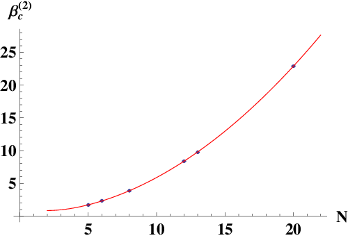
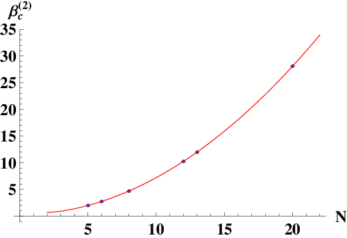
For the critical couplings at the second transition, , where determinations for many values of are available, we tried to find a simple scaling dependence with at fixed . Taking inspiration from Ref. [9], we made a few attempts and found that a good fit is achieved with the function
In Table 2 we report the values of the parameters and for , while Figs. 1 shows the fitting functions against numerical data.
Inspecting the behavior of the coefficient in Table 2, one observes that it approaches its zero-temperature limit when increases [3]. We have investigated this approach in details and found that it can be well described by the following fitting function: . The results of the fits are given in Table 3 and Figs. 2. It can be seen both from the given in the table and from the plots that describes data better than .
| 2 | 1.1194(11) | 0.141(24) | 209 |
|---|---|---|---|
| 4 | 1.37440(60) | -0.0046(88) | 18.2 |
| 8 | 1.45745(57) | 0.0155(53) | 16.1 |

| 1.050(25) | 0.67 | 95.0 |
| 1.1220(67) | 0.64 | 6.12 |
| 1.140(17) | 0.6331(61) | 5.42 |


3.3 Continuum limit
Finding the continuum limit of the finite temperature theory in the first or in the second transition amounts to extrapolate the corresponding critical couplings, or , to the limit at fixed .
The theory of dimensional cross-over [5] suggests the fitting function to be used:
| (10) |
where and are the critical couplings and the critical index of the zero-temperature theory. Since we know that, for any , the LGT at zero-temperature exhibits only one phase transition, with the critical index depending on the side from which the transition is approached [3], we expect that, for a given , the fit parameters and take the same value and agree with the zero-temperature critical coupling at the same . As for the fit parameter , we expect it to agree with the value of the critical index at one of the two sides of the zero-temperature transition.
We fitted with the function given in (10) our data for the critical couplings at =5,6,8,12,13,20 (see Tables 4 and 5) and for the critical couplings at =5 (see Table 6). In some cases in the fit we fixed either or , or both, at the values known from the zero-temperature theory [3]. The scenario which emerges from the inspection of Tables 4, 5 and 6 is that, despite the large reduced chi-squared obtained in a few cases, the agreement between the fit parameters and the known zero-temperature critical couplings [3] is satisfactory. As for the value of the fit parameter , results are not precise enough to discriminate between the known values of the critical index of the zero-temperature theory at one or the other side of the transition [3].
This analysis allows us for the determination of the critical temperature in the continuum limit for all the values of considered in this work.
| 0.868(-) | 2.23055(-) | 0.877(-) | - | |
| 0.813(27) | 2.177(12) | 0.670 | 158 | |
| 0.803(30) | 2.170(14) | 0.640 | 223 | |
| 5 | 0.825(38) | 2.17961 | 0.692(45) | 131 |
| 0.810(13) | 2.17961 | 0.670 | 81.8 | |
| 0.776(31)∗ | 2.17961 | 0.670 | 74.2∗ | |
| 0.789(17) | 2.17961 | 0.640 | 161 | |
| 0.731(18)∗ | 2.17961 | 0.640 | 31.4∗ | |
| 0.6814(-) | 3.04317(-) | 0.876(-) | - | |
| 0.6769(76) | 2.977(10) | 0.674 | 5.02 | |
| 0.6740(85) | 2.969(12) | 0.642 | 6.90 | |
| 6 | 0.6832(46) | 3.00683 | 0.768(15) | 1.14 |
| 0.6573(47) | 3.00683 | 0.674 | 22.6 | |
| 0.572(13)∗ | 3.00683 | 0.674 | 1.44∗ | |
| 0.6487(60) | 3.00683 | 0.642 | 40.6 | |
| 0.542(21)∗ | 3.00683 | 0.642 | 4.48∗ | |
| 0.42330(-) | 5.14422(-) | 0.674(-) | - | |
| 0.42378(12) | 5.14299(25) | 0.672 | 0.19 | |
| 0.4316(22) | 5.1225(46) | 0.637 | 66.5 | |
| 8 | 0.4294(12) | 5.12829 | 0.648(6) | 33.0 |
| 0.4287(39) | 5.12829 | 0.672 | 321 | |
| 0.4427(39)∗ | 5.12829 | 0.672 | 177∗ | |
| 0.4298(19) | 5.12829 | 0.637 | 86.1 | |
| 0.4216(10)∗ | 5.12829 | 0.637 | 2.21∗ |
| 0.24728(-) | 11.2566(-) | 0.674(-) | - | |
| 0.24559(13) | 11.2640(23) | 0.670 | 0.22 | |
| 0.25615(72) | 11.218(12) | 0.640 | 6.18 | |
| 12 | 0.2602(32) | 11.1962 | 0.630(11) | 14.2 |
| 0.24954(28) | 11.1962 | 0.670 | 89.8 | |
| 0.2619(87)∗ | 11.1962 | 0.670 | 55.5∗ | |
| 0.25742(10) | 11.1962 | 0.640 | 12.7 | |
| 0.2597(51)∗ | 11.1962 | 0.640 | 21.3∗ | |
| 0.22433(-) | 13.1391(-) | 0.654(-) | - | |
| 0.21872(53) | 13.1656(56) | 0.671 | 5.88 | |
| 0.22851(40) | 13.1199(42) | 0.642 | 3.40 | |
| 13 | 0.2310(12) | 13.1077 | 0.635(4) | 8.86 |
| 0.2225(30) | 13.1077 | 0.671 | 314 | |
| 0.2342(62)∗ | 13.1077 | 0.671 | 113∗ | |
| 0.22928(67) | 13.1077 | 0.642 | 16.0 | |
| 0.2311(24)∗ | 13.1077 | 0.642 | 19.2∗ | |
| 0.144857(-) | 30.5427(-) | 0.608(-) | - | |
| 0.1297(37) | 30.73(10) | 0.673 | 147 | |
| 0.1356(24) | 30.658(64) | 0.647 | 58.8 | |
| 20 | 0.1357(26) | 30.6729 | 0.642(19) | 58.2 |
| 0.13171(98) | 30.6729 | 0.673 | 97.3 | |
| 0.13199(13)∗ | 30.6729 | 0.673 | 1.57∗ | |
| 0.13506(54) | 30.6729 | 0.647 | 31.0 | |
| 0.13519(49)∗ | 30.6729 | 0.647 | 23.9∗ |
| 0.790(5) | 2.198(9) | 0.84(3) | 1.21 | |
| 0.764(14) | 2.144(9) | 0.670 | 23.1 | |
| 0.758(16) | 2.135(11) | 0.640 | 33.6 | |
| 5 | 0.786(7) | 2.17961 | 0.788(10) | 2.66 |
| 0.722(16) | 2.17961 | 0.670 | 105 | |
| 0.709(19) | 2.17961 | 0.640 | 171 |
3.4 Critical indices
Some critical indices at the two transitions in the LGT at finite temperature can be extracted by the standard FSS analysis. In particular, the behavior on the lattice size of the standard magnetization and of its susceptibility at the second transition allows to extract the indices and through a fit with the functions
| (11) |
Similarly, the behavior on of the rotated magnetization and of its susceptibility at the first transition point allow the extraction of the same critical indices at that transition.
Thereafter, the hyperscaling relation can be checked and the magnetic index can be extracted at both transitions.
Our results are summarized in Tables 7 and 8. We can see that the hyperscaling relation is generally satisfied and the critical index generally takes values compatible with 1/4 at the second transition and with at the first transition, in agreement with the expectations.
| 5 | 2 | 1.617(2) | 0.097(6) | 0.101 | 1.847(5) | 0.561 | 2.04(2) | 0.153(5) |
|---|---|---|---|---|---|---|---|---|
| 5 | 4 | 1.943(2) | 0.11(1) | 1.25 | 1.841(1) | 0.70 | 2.07(3) | 0.159(1) |
| 5 | 8 | 2.085(2) | 0.09(2) | 0.77 | 1.844(1) | 0.78 | 2.01(4) | 0.156(1) |
| 8 | 4 | 2.544(8) | 0.26(2) | 1.79 | 1.930(3) | 1.58 | 1.41(5) | 0.070(3) |
| 8 | 8 | 3.422(9) | 0.52(5) | 0.21 | 1.959(1) | 0.21 | 0.9(1) | 0.040(1) |
| 13 | 2 | 1.795(4) | 0.07(5) | 1.28 | 1.968(9) | 0.97 | 2.1(1) | 0.032(9) |
| 13 | 4 | 2.74(5) | 0.26(2) | 1.81 | 1.976(3) | 1.80 | 1.5(1) | 0.024(3) |
| 13 | 8 | 3.358(7) | 0.9(1) | 1.17 | 1.973(4) | 1.25 | 0.3(2) | 0.027(4) |
| 20 | 4 | 2.57(1) | 0.25(2) | 0.37 | 1.991(3) | 1.91 | 1.49(5) | 0.009(3) |
| 20 | 8 | 3.42(5) | 0.72(6) | 0.41 | 1.9790(16) | 0.33 | 0.55(13) | 0.0210(16) |
| 5 | 2 | 1.6972(14) | 0.1259(2) | 1.22 | 1.750(3) | 0.50 | 2.001(4) | 0.250(3) |
|---|---|---|---|---|---|---|---|---|
| 5 | 4 | 1.9885(15) | 0.1061(3) | 2.67 | 1.758(9) | 2.45 | 1.971(9) | 0.242(9) |
| 5 | 8 | 2.1207(9) | 0.1376(6) | 2.04 | 1.747(15) | 1.62 | 2.022(16) | 0.253(15) |
| 6 | 2 | 2.3410(15) | 0.26(3) | 1.8 | 1.6(6) | 1.21 | 2.1(6) | 0.4(6) |
| 6 | 4 | 2.725(12) | 0.1056(13) | 1.84 | 1.76(7) | 2.05 | 1.97(8) | 0.24(7) |
| 6 | 8 | 2.899(4) | 0.0949(4) | 1.67 | 1.731(8) | 0.71 | 1.920(9) | 0.269(8) |
| 8 | 2 | 3.8640(10) | 0.1336(4) | 0.36 | 1.743(15) | 0.73 | 2.010(16) | 0.257(15) |
| 8 | 4 | 4.6864(15) | 0.1278(4) | 3.85 | 1.753(6) | 1.34 | 2.009(7) | 0.247(6) |
| 8 | 8 | 4.9808(5) | 0.1379(5) | 0.77 | 1.745(18) | 1.82 | 2.020(19) | 0.255(18) |
| 12 | 2 | 8.3745(5) | 0.1283(16) | 1.22 | 1.73(4) | 0.78 | 1.99(4) | 0.27(4) |
| 12 | 4 | 10.240(7) | 0.1303(4) | 1.52 | 1.746(9) | 0.87 | 2.007(10) | 0.254(9) |
| 12 | 8 | 10.898(5) | 0.149(3) | 0.64 | 1.78(16) | 1.19 | 2.07(17) | 0.22(16) |
| 13 | 2 | 9.735(4) | 0.1251(2) | 0.22 | 1.744(5) | 0.09 | 1.995(5) | 0.256(5) |
| 13 | 4 | 11.959(6) | 0.1265(2) | 1.43 | 1.746(3) | 0.48 | 1.999(4) | 0.254(3) |
| 13 | 8 | 12.730(2) | 0.1357(18) | 3.55 | 1.75(2) | 0.82 | 2.02(2) | 0.25(2) |
| 20 | 2 | 22.87(4) | 0.1322(14) | 1.06 | 1.78(3) | 0.68 | 2.04(4) | 0.22(3) |
| 20 | 4 | 28.089(3) | 0.1384(4) | 0.17 | 1.748(14) | 0.17 | 2.025(15) | 0.252(14) |
| 20 | 8 | 29.758(6) | 0.1278(7) | 1.60 | 1.713(17) | 1.15 | 1.968(18) | 0.287(17) |
Finally, the critical index at the second transition was estimated following a procedure inspired by Ref. [8]: first, for each lattice size the known function is used to determine ; then, from this, the derivative of with respect to the rescaled coupling can be calculated,
| (12) |
The best estimate of is found by minimizing the deviation of with respect to a constant value. The minimization was done at . The resulting values for , summarized in Table 9, exhibit a fair agreement with the expected BKT value 1/2, sometimes within large error bars.
| 5 | 2 | 0.55(9) | 1.06 |
|---|---|---|---|
| 5 | 4 | 7.89 | |
| 5 | 8 | 0.46(4) | 0.51 |
| 6 | 2 | - | - |
| 6 | 4 | 0.5(2) | 0.42 |
| 6 | 8 | 0.57(10) | 0.20 |
| 8 | 2 | 0.63(5) | 0.16 |
| 8 | 4 | 0.52(16) | 1.01 |
| 8 | 8 | 0.42(3) | 1.32 |
| 12 | 2 | 0.41(13) | 0.018 |
| 12 | 4 | 0.60(8) | 0.20 |
| 12 | 8 | 0.33(1) | 0.008 |
| 13 | 2 | 3.27 | |
| 13 | 4 | 0.62(9) | 0.34 |
| 13 | 8 | 0.43(3) | 0.83 |
| 20 | 2 | 0.60(12) | 0.39 |
| 20 | 4 | 0.57(4) | 0.05 |
| 20 | 8 | 0.39(2) | 0.13 |
4 Summary
This paper completes our study of the critical behavior of lattice gauge theories both at zero and at finite temperatures. In order to accomplish this investigation, we have used various methods like renormalization group, duality transformations and Monte Carlo simulations, combined with finite-size scaling. Here we would like to outline our main findings and list some open problems left for future investigation.
The main results can be shortly summarized as follows.
- •
We have found that in all vector models two BKT-like phase transitions occur at finite temperatures if . In this paper we have extended the results of Ref. [2] for and to other values of and to . In all cases studied, the results for the critical indices suggest that finite-temperature lattice models belong to the universality class of two-dimensional vector spin models, in agreement with the Svetitsky-Yaffe conjecture. Furthermore, the available results for many values of allowed us to propose and check some scaling formulas for the critical point of the second phase transition. Combining the results of the present paper with those for the index obtained by us at zero temperature in Ref. [3] enabled us to check the continuum scaling and to predict the approximate value for in the continuum limit.
- •
Three-dimensional models at zero temperature exhibit a single phase transition which appears to be of 3rd order if one approaches the critical point from above and belongs to the universality class of the model. However, if one approaches the critical point from below, the index is compatible with the value of the Ising model. This suggests that the free energy develops a cusp in the large volume limit which leads to different singularities. A very interesting feature of all models at large is the existence of a symmetric phase on the finite lattice which manifests itself in the characteristic behavior of the scatter plots for magnetization of the dual spins.
The most interesting open problems, on our opinion, are the following.
- •
More precise determination of critical points and indices at the 1st BKT transition for and establishing the formula for the scaling of these critical points with .
- •
What is the physics behind the two BKT transitions? Most probably it is related to the existence of two topological excitations dual to each other. This would be similar to what happens in spin models. Unfortunately, the analytical proof of this is still to be constructed.
- •
A very intriguing problem is the physics of symmetric phase at zero temperature. In particular, it is not clear if this phase survives the transition to the thermodynamical limit and how it is connected to the massless BKT phase at finite temperature.
5 Acknowledgments
The work of the Ukrainian co-authors was supported by the Ukrainian State Fund for Fundamental Researches under the grant F58/384-2013. Numerical simulations have been partly carried out on Ukrainian National GRID facilities. O.B. thanks for warm hospitality the Dipartimento di Fisica dell’Università della Calabria and the INFN Gruppo Collegato di Cosenza during the final stages of this investigation. This work has been partially supported by the INFN SUMA project.
References
- [1] O. Borisenko, V. Chelnokov, G. Cortese, R. Fiore, M. Gravina, A. Papa, I. Surzhikov, Phys. Rev. E 86 (2012) 051131; PoS LATTICE 2012 270 [arXiv:1212.1051 [hep-lat]].
- [2] O. Borisenko, V. Chelnokov, G. Cortese, M. Gravina, A. Papa, I. Surzhikov, Nucl. Phys. B 870 (2013) 159; PoS LATTICE 2013 463 [arXiv:1310.1039 [hep-lat]].
- [3] O. Borisenko, V. Chelnokov, G. Cortese, M. Gravina, A. Papa, I. Surzhikov, Nucl. Phys. B 879 (2014) 80; PoS LATTICE 2013 347 [arXiv:1311.0471 [hep-lat]].
- [4] B. Svetitsky, L. Yaffe, Nucl. Phys. B 210 (1982) 423.
- [5] M. Caselle, M. Hasenbusch, M. Panero, JHEP 0301 (2003) 057; M. Caselle, M. Hasenbusch, Nucl. Phys. B 470 (1996) 435.
- [6] S. Elitzur, R.B. Pearson, J. Shigemitsu, Phys. Rev. D 19 (1979) 3698.
- [7] A. Ukawa, P. Windey, A.H. Guth, Phys. Rev. D 21 (1980) 1013.
- [8] M. Campostrini, M. Hasenbusch, A. Pelissetto, P. Rossi, E. Vicari, Phys. Rev. B 63 (2001) 214503.
- [9] G. Bhanot and M. Creutz, Phys. Rev. D 21 (1980) 2892.