跳到论文正文
W Papers独立论文阅读器 arXiv:1408.2500 论文正文 计算阅读时间 · 0%
引用这篇论文根据当前论文元数据生成,正式投稿前建议核对。


License: arXiv.org perpetual non-exclusive license
arXiv:1408.2500v1 [hep-ph] 11 Aug 2014

Four-dimensional formulation of the sector-improved residue subtraction scheme

Journal: Nuclear Physics B
M. Czakon and D. Heymes Address:  Institute for Theoretical Particle Physics and Cosmology, RWTH Aachen University, D-52056 Aachen, Germany
Abstract

Four years ago, one of us introduced a novel subtraction scheme [1] for the evaluation of double-real radiation contributions to cross sections at next-to-next-to-leading order (NNLO) in QCD. This approach, named SecToR Improved Phase sPacE for Real radiation (STRIPPER), has already found several non-trivial applications. In particular, it has allowed for the determination of NNLO corrections to hadronic top-quark pair production, fully differential top-quark decays, inclusive semileptonic charmless b-quark decays, associated Higgs boson and jet production in gluon fusion, muon decay spin asymmetry, and t-channel single-top production. Common to these calculations was the use of conventional dimensional regularization (CDR). In this publication, we present a complete formulation of the subtraction scheme for arbitrary processes with any number of colored partons in the final state, and up to two partons in the initial state. Furthermore, we modify the integrated subtraction terms of the double-real radiation to enable the introduction of the ’t Hooft-Veltman version of dimensional regularization (HV), in which resolved states are four-dimensional. We demonstrate the correctness of our approach on the example of top-quark pair production in the gluon fusion channel.

1 Introduction

Perturbative calculations beyond the next-to-leading order of Quantum Chromodynamics are notorious for their complexity. Already the next-to-next-to-leading order presents tremendous obstacles. One of them is the evaluation of infrared and ultraviolet divergent two-loop virtual amplitudes. This is an unsolved issue in the general case despite the existence of a few analytic results for low multiplicity processes. Another obstacle is the evaluation of double-real and mixed real-virtual contributions containing infrared singular phase space integrals. In principle, these contributions can be obtained by means of Monte Carlo techniques, once suitable subtractions have been introduced to generate numerically integrable functions. The form of the subtractions defines a subtraction scheme. Unfortunately, it turns out that subtraction schemes are extremely complex. At present, there are several on-going multi-year efforts at the construction of general solutions. Antenna subtraction [2], and qTq_{T} subtraction [3], are amongst the most advanced initiatives, which have already found several non-trivial applications. Another scheme under construction has been introduced in Ref. [4]. Here, we will be concerned with the subtraction scheme STRIPPER introduced by one of us in Ref. [1]. Inspired in some aspects by ideas of Frixione, Kunszt and Signer [5], and in other aspects by ideas of Binoth and Heinrich [6], the scheme has proven its worth in many applications: it has allowed for the determination of NNLO corrections to hadronic top-quark pair production [7, 8, 9, 10, 11], fully differential top-quark decays [12], inclusive semileptonic charmless b-quark decays [13], associated Higgs boson and jet production in gluon fusion [14], muon decay spin asymmetry [15], and t-channel single-top production [16]. The listed advanced STRIPPER applications performed independently of the inventor have been preceded by the much simpler case of QED corrections to ZZ-boson decay into a pair of massless leptons [17]. The purpose of the present work is to complete the construction of the scheme in order to allow for the evaluation of cross sections for arbitrary processes.

The original idea of Ref. [1] was to concentrate on the numerical calculation of the coefficients of the Laurent expansion in ϵ\epsilon (dimensional regularization parameter, with space-time dimension d=4−2​ϵd=4-2\epsilon) of the double-real cross section contribution. The latter requires a phase space integral over the momenta not only of the partons present in the Born approximation, but also of two additional massless partons. It seemed obvious that other cross section contributions are much easier to obtain, since their kinematics is, in the worst case, the same as that of next-to-leading order real-radiation contributions. Furthermore, the concept was to refrain from (almost) any analytic integration. By inspection of other efforts, it was clear that it is the insistence on analytic integration that makes the subtraction schemes difficult to develop. Finally, in order to avoid as many complications as possible, the construction was performed uniformly in dd dimensions. This corresponds to conventional dimensional regularization, where both momenta and spin degrees-of-freedom of external particles are dd dimensional. This implies that even Born matrix elements will have a non-trivial expansion in ϵ\epsilon. While the other basic ideas of the scheme stood the test of time, the use of CDR is now an important drawback. Indeed, software implementations of tree-level matrix elements only provide them at ϵ=0\epsilon=0, i.e. in four dimensions. This makes it necessary to recalculate the matrix elements for each project from scratch. Furthermore, the need to parameterize an increasing number of dimensions depending on the multiplicity of the process seems not only a major annoyance, but also a source of inefficiency. In this publication, we will solve the problem by introducing a number of corrections to the integrated subtraction terms in the double-real radiation contribution. As a result, we will formulate the scheme in ’t Hooft-Veltman regularization. In particular, we will only need four-dimensional external momenta and polarizations in the evaluation of actual matrix elements. There will still be a trace of higher dimensionality in the integration over unresolved momenta. However, we will only have to consider six dimensional unresolved momenta in the worst case. On the example of top-quark pair production, we will also demonstrate that the introduced improvements of STRIPPER fulfill their purpose. We stress that we only present the algorithm to obtain the expressions needed for the implementation of the subtraction scheme. This algorithm requires the knowledge of soft and collinear limits of QCD amplitudes and provides the expressions for the subtraction and integrated subtraction terms by simple substitutions. Due to the number and size of the resulting final formulae, we do not reproduce them here. Instead, we plan to provide a software package in the future. Nevertheless, existing calculations can be converted to ’t Hooft-Veltman regularization with moderate effort following this publication.

The paper is organized as follows. In the next section, we present an outline of the subtraction scheme together with a complete list of cross section contributions to evaluate in a general next-to-next-to-leading order calculation. Subsequently, we proceed with the construction of the scheme by considering its major elements: phase space decomposition (Section 3), phase space parameterization (Section 4), and derivation of the subtraction and integrated subtraction terms (Section 5). This part is common to the CDR and HV formulations. Afterwards, we discuss the modifications necessary to introduce HV regularization: average over the azimuthal angles (Section 6), separation of finite contributions (Section 7), and finally the regularization itself (Section 8). This part is followed by the example of top-quark pair production in the gluon fusion channel (Section 9). The main text is closed with conclusions. Appendices form an important part of the publication. They are self-contained, and the information provided therein is sufficient to construct the complete subtraction scheme in the most general case. Our notation is summarized in A. Spherical angles in dd dimensions are discussed in B. Divergences of virtual amplitudes are considered in C, whereas limits of amplitudes are contained in D and E. F contains the well-known Altarelli-Parisi splitting kernels necessary for initial-state collinear renormalization of partonic cross sections.

2 Outline of the subtraction scheme

We are interested in the calculation of next-to-next-to-leading order QCD corrections to scattering cross sections. The subtraction scheme we will describe can also be used for decay processes, since the phase space integrals present there share the same structure. The formulae below would only have to be trivially modified. Furthermore, it is possible to include QED corrections by a modification of the color algebra (see A). We will not discuss this issue in any more detail. We now need to specify the possible initial and final states. At present, the most relevant case is hadron-hadron scattering. Therefore, we will give expressions with this class of processes in mind. Nevertheless, we will separate the hadron scale physics from the parton scale physics. Indeed, we will only ever manipulate partonic cross sections. This makes it possible to include lepton-hadron and lepton-lepton scattering processes by simply removing factorization contributions. As far as the final state is concerned, we only require that there be at least two particles at the Born level. The reason is that in the special case of a single particle, the partonic cross section becomes a distribution, and we assume that we can work with ordinary functions only. In the following, we will concentrate on external partons carrying a color charge. Any additional particles, which are not charged under the color gauge group play no role whatsoever in the construction of the scheme, and can be trivially included in the phase space integrals.

The hadronic cross section is known to factorize into a convolution of parton distribution functions and the renormalized partonic cross section

σh1​h2​(P1,P2)=∑a​b∬01d​x1​d​x2​fa/h1​(x1,μF2)​fb/h2​(x2,μF2)​σ^a​b​(x1​P1,x2​P2,αs​(μR2),μR2,μF2),\sigma_{h_{1}h_{2}}(P_{1},P_{2})=\sum_{ab}\iint_{0}^{1}\mathrm{d}x_{1}\mathrm{d}x_{2}\,f_{a/h_{1}}(x_{1},\mu^{2}_{F})\,f_{b/h_{2}}(x_{2},\mu^{2}_{F})\,\hat{\sigma}_{ab}(x_{1}P_{1},x_{2}P_{2};\,{\alpha_{s}}(\mu^{2}_{R}),\,\mu^{2}_{R},\,\mu^{2}_{F})\;, (1)

where P1,2P_{1,2} are the momenta of the hadrons h1,2h_{1,2}, and fa/h​(x,μF2)f_{a/h}(x,\mu^{2}_{F}) is the parton distribution function (PDF) of parton aa within the hadron hh, at the factorization scale μF\mu_{F}. In the following, p1,2=x1,2​P1,2p_{1,2}=x_{1,2}P_{1,2} will denote the parton momenta. If we are able to numerically evaluate the partonic cross section, σ^a​b\hat{\sigma}_{ab}, for an arbitrary initial-state energy, then we can also obtain the hadronic cross section by an additional integration over the parton momentum fractions. This is the reason, why the construction of the subtraction scheme will never make reference to the initial-state hadrons, but only to the initial-state partons. The partonic cross section can be expanded in a series in αs​(μR2){\alpha_{s}}(\mu^{2}_{R}), where μR\mu_{R} is the renormalization scale. Up to next-to-next-to-leading order (NNLO) it reads

σ^a​b=σ^a​b(0)+σ^a​b(1)+σ^a​b(2).\hat{\sigma}_{ab}=\hat{\sigma}^{(0)}_{ab}+\hat{\sigma}^{(1)}_{ab}+\hat{\sigma}^{(2)}_{ab}\;. (2)

Each term of the expansion can be further decomposed according to the multiplicity of the final state. At leading order

σ^a​b(0)=σ^a​bB=12​s^​1Na​b​∫d​𝚽n​⟨ℳn(0)|ℳn(0)⟩​Fn,\hat{\sigma}^{(0)}_{ab}=\hat{\sigma}^{\mathrm{B}}_{ab}=\frac{1}{2\hat{s}}\frac{1}{N_{ab}}\int\mathrm{d}\bm{\Phi}_{n}\,\langle\mathcal{M}_{n}^{(0)}|\mathcal{M}_{n}^{(0)}\rangle\,\mathrm{F}_{n}\;, (3)

where s^=(p1+p2)2\hat{s}=(p_{1}+p_{2})^{2} is the square of the partonic center-of-mass energy, while Na​bN_{ab} is the spin and color average factor, defined as the product of the number of spin and color degrees of freedom of the partons aa and bb. The subscript nn points to the number of final states in this contribution. The notation and normalization of phase spaces and matrix elements is specified in A. Fn\mathrm{F}_{n} is the measurement function defining the observable. It is a function of the final state momenta and flavors. Up to the next-to-next-to-leading order, we need three such functions, FnF_{n}, Fn+1F_{n+1} and Fn+2F_{n+2}. They must fulfill the requirements of infrared safety, i.e. if the energy of a final state parton vanishes, or if the parton becomes collinear to another one, then Fn+m→Fn+m−1F_{n+m}\to F_{n+m-1} for m>0m>0 and Fn→0F_{n}\to 0.

At next-to-leading order there is

σ^a​b(1)=σ^a​bR+σ^a​bV+σ^a​bC,\hat{\sigma}^{(1)}_{ab}=\hat{\sigma}^{\mathrm{R}}_{ab}+\hat{\sigma}^{\mathrm{V}}_{ab}+\hat{\sigma}^{\mathrm{C}}_{ab}\;, (4)

with

σ^Ra​b=12​s^1Na​b∫d𝚽n+1⟨ℳn+1(0)|ℳn+1(0)⟩Fn+1,σ^Va​b=12​s^1Na​b∫d𝚽n 2Re⟨ℳn(0)|ℳn(1)⟩Fn,σ^a​bC​(p1,p2)=αs2​π​1ϵ​(μR2μF2)ϵ​∑c∫01d​z​[Pc​a(0)​(z)​σ^c​bB​(z​p1,p2)+Pc​b(0)​(z)​σ^a​cB​(p1,z​p2)],\begin{gathered}\hat{\sigma}^{\mathrm{R}}_{ab}=\frac{1}{2\hat{s}}\frac{1}{N_{ab}}\int\mathrm{d}\bm{\Phi}_{n+1}\,\langle\mathcal{M}_{n+1}^{(0)}|\mathcal{M}_{n+1}^{(0)}\rangle\,\mathrm{F}_{n+1}\;,\quad\hat{\sigma}^{\mathrm{V}}_{ab}=\frac{1}{2\hat{s}}\frac{1}{N_{ab}}\int\mathrm{d}\bm{\Phi}_{n}\,2\mathrm{Re}\,\langle\mathcal{M}_{n}^{(0)}|\mathcal{M}_{n}^{(1)}\rangle\,\mathrm{F}_{n}\;,\\[5.69046pt] \hat{\sigma}^{\mathrm{C}}_{ab}(p_{1},p_{2})=\frac{{\alpha_{s}}}{2\pi}\frac{1}{\epsilon}\left(\frac{\mu^{2}_{R}}{\mu^{2}_{F}}\right)^{\epsilon}\sum_{c}\int_{0}^{1}\mathrm{d}z\left[P^{(0)}_{ca}(z)\,\hat{\sigma}^{\mathrm{B}}_{cb}(zp_{1},p_{2})+P^{(0)}_{cb}(z)\,\hat{\sigma}^{\mathrm{B}}_{ac}(p_{1},zp_{2})\right]\;,\end{gathered} (5)

where the splitting functions required are reproduced in F. Finally, at next-to-next-to-leading order, we have

σ^a​b(2)=σ^a​bRR+σ^a​bRV+σ^a​bVV+σ^a​bC1+σ^a​bC2,\hat{\sigma}^{(2)}_{ab}=\hat{\sigma}^{\mathrm{RR}}_{ab}+\hat{\sigma}^{\mathrm{RV}}_{ab}+\hat{\sigma}^{\mathrm{VV}}_{ab}+\hat{\sigma}^{\mathrm{C1}}_{ab}+\hat{\sigma}^{\mathrm{C2}}_{ab}\;, (6)

with

σ^RRa​b=12​s^1Na​b∫d𝚽n+2⟨ℳn+2(0)|ℳn+2(0)⟩Fn+2,σ^RVa​b=12​s^1Na​b∫d𝚽n+1 2Re⟨ℳn+1(0)|ℳn+1(1)⟩Fn+1,σ^a​bVV=12​s^​1Na​b​∫d​𝚽n​(2​Re​⟨ℳn(0)|ℳn(2)⟩+⟨ℳn(1)|ℳn(1)⟩)​Fn,\begin{gathered}\hat{\sigma}^{\mathrm{RR}}_{ab}=\frac{1}{2\hat{s}}\frac{1}{N_{ab}}\int\mathrm{d}\bm{\Phi}_{n+2}\,\langle\mathcal{M}_{n+2}^{(0)}|\mathcal{M}_{n+2}^{(0)}\rangle\,\mathrm{F}_{n+2}\;,\quad\hat{\sigma}^{\mathrm{RV}}_{ab}=\frac{1}{2\hat{s}}\frac{1}{N_{ab}}\int\mathrm{d}\bm{\Phi}_{n+1}\,2\mathrm{Re}\,\langle\mathcal{M}_{n+1}^{(0)}|\mathcal{M}_{n+1}^{(1)}\rangle\,\mathrm{F}_{n+1}\;,\\[5.69046pt] \hat{\sigma}^{\mathrm{VV}}_{ab}=\frac{1}{2\hat{s}}\frac{1}{N_{ab}}\int\mathrm{d}\bm{\Phi}_{n}\,\Big(2\mathrm{Re}\,\langle\mathcal{M}_{n}^{(0)}|\mathcal{M}_{n}^{(2)}\rangle+\langle\mathcal{M}_{n}^{(1)}|\mathcal{M}_{n}^{(1)}\rangle\Big)\,\mathrm{F}_{n}\;,\end{gathered} (7)

and

σ^a​bC1​(p1,p2)=αs2​π​1ϵ​(μR2μF2)ϵ​∑c∫01d​z​[Pc​a(0)​(z)​σ^c​bR​(z​p1,p2)+Pc​b(0)​(z)​σ^a​cR​(p1,z​p2)],σ^a​bC2​(p1,p2)=αs2​π​1ϵ​(μR2μF2)ϵ​∑c∫01d​z​[Pc​a(0)​(z)​σ^c​bV​(z​p1,p2)+Pc​b(0)​(z)​σ^a​cV​(p1,z​p2)]+(αs2​π)212​ϵ(μR2μF2)2​ϵ∑c∫01dz[P(1)c​a(z)σ^Bc​b(zp1,p2)+P(1)c​b(z)σ^Ba​c(p1,zp2)]+(αs2​π)2β04​ϵ2[(μR2μF2)2​ϵ−2(μR2μF2)ϵ]∑c∫01dz[P(0)c​a(z)σ^Bc​b(zp1,p2)+P(0)c​b(z)σ^Ba​c(p1,zp2)]+(αs2​π)212​ϵ2(μR2μF2)2​ϵ∑c​d∫01dz[(P(0)c​d⊗P(0)d​a)(z)σ^Bc​b(zp1,p2)+(P(0)c​d⊗P(0)d​b)(z)σ^Ba​c(p1,zp2)]+(αs2​π)21ϵ2(μR2μF2)2​ϵ∑c​d∬01dzdz¯[P(0)c​a(z)P(0)d​b(z¯)σ^Bc​d(zp1,z¯p2)],\begin{split}\hat{\sigma}^{\mathrm{C1}}_{ab}(p_{1},p_{2})&=\frac{{\alpha_{s}}}{2\pi}\frac{1}{\epsilon}\left(\frac{\mu^{2}_{R}}{\mu^{2}_{F}}\right)^{\epsilon}\sum_{c}\int_{0}^{1}\mathrm{d}z\left[P^{(0)}_{ca}(z)\,\hat{\sigma}^{\mathrm{R}}_{cb}(zp_{1},p_{2})+P^{(0)}_{cb}(z)\,\hat{\sigma}^{\mathrm{R}}_{ac}(p_{1},zp_{2})\right]\;,\\[5.69046pt] \hat{\sigma}^{\mathrm{C2}}_{ab}(p_{1},p_{2})&=\frac{{\alpha_{s}}}{2\pi}\frac{1}{\epsilon}\left(\frac{\mu^{2}_{R}}{\mu^{2}_{F}}\right)^{\epsilon}\sum_{c}\int_{0}^{1}\mathrm{d}z\left[P^{(0)}_{ca}(z)\,\hat{\sigma}^{\mathrm{V}}_{cb}(zp_{1},p_{2})+P^{(0)}_{cb}(z)\,\hat{\sigma}^{\mathrm{V}}_{ac}(p_{1},zp_{2})\right]\\ &+\left(\frac{{\alpha_{s}}}{2\pi}\right)^{2}\frac{1}{2\epsilon}\left(\frac{\mu^{2}_{R}}{\mu^{2}_{F}}\right)^{2\epsilon}\sum_{c}\int_{0}^{1}\mathrm{d}z\left[P^{(1)}_{ca}(z)\,\hat{\sigma}^{\mathrm{B}}_{cb}(zp_{1},p_{2})+P^{(1)}_{cb}(z)\,\hat{\sigma}^{\mathrm{B}}_{ac}(p_{1},zp_{2})\right]\\ &+\left(\frac{{\alpha_{s}}}{2\pi}\right)^{2}\frac{\beta_{0}}{4\epsilon^{2}}\left[\left(\frac{\mu^{2}_{R}}{\mu^{2}_{F}}\right)^{2\epsilon}-2\left(\frac{\mu^{2}_{R}}{\mu^{2}_{F}}\right)^{\epsilon}\right]\sum_{c}\int_{0}^{1}\mathrm{d}z\left[P^{(0)}_{ca}(z)\,\hat{\sigma}^{\mathrm{B}}_{cb}(zp_{1},p_{2})+P^{(0)}_{cb}(z)\,\hat{\sigma}^{\mathrm{B}}_{ac}(p_{1},zp_{2})\right]\\ &+\left(\frac{{\alpha_{s}}}{2\pi}\right)^{2}\frac{1}{2\epsilon^{2}}\left(\frac{\mu^{2}_{R}}{\mu^{2}_{F}}\right)^{2\epsilon}\sum_{cd}\int_{0}^{1}\mathrm{d}z\left[\Big(P^{(0)}_{cd}\otimes P^{(0)}_{da}\Big)(z)\,\hat{\sigma}^{\mathrm{B}}_{cb}(zp_{1},p_{2})+\Big(P^{(0)}_{cd}\otimes P^{(0)}_{db}\Big)(z)\,\hat{\sigma}^{\mathrm{B}}_{ac}(p_{1},zp_{2})\right]\\ &+\left(\frac{{\alpha_{s}}}{2\pi}\right)^{2}\frac{1}{\epsilon^{2}}\left(\frac{\mu^{2}_{R}}{\mu^{2}_{F}}\right)^{2\epsilon}\sum_{cd}\iint_{0}^{1}\mathrm{d}z\,\mathrm{d}\bar{z}\left[P^{(0)}_{ca}(z)\,P^{(0)}_{db}({\bar{z}})\,\hat{\sigma}^{\mathrm{B}}_{cd}(zp_{1},\bar{z}p_{2})\right]\;,\end{split} (8)

where

(f⊗g)​(x)=∬01d​y​𝑑z​f​(y)​g​(z)​δ​(x−y​z).\left(f\otimes g\right)(x)=\iint_{0}^{1}\mathrm{d}y\,\mathrm{d}z\,f(y)g(z)\,\delta(x-yz)\;. (9)

In general, it is only possible to evaluate the cross section contributions listed above using numerical Monte Carlo integration methods. Unfortunately, phase spaces with n+1n+1 and n+2n+2 final states contain infrared singular configurations, which are regulated with dimensional regularization. The latter, if applied naively, spoils the stability of the numerics, since a limit has to be taken once all contributions are combined. This problem is resolved with a subtraction scheme, which extracts the explicit singularities and provides integrable functions, which do not depend on the parameter of dimensional regularization.

The idea behind the construction of the subtraction scheme STRIPPER is to derive Laurent expansions in ϵ\epsilon for each of the cross section contributions independently. The basic algorithm has three stages:

phase space decomposition (Section 3):

phase spaces with n+1n+1 and n+2n+2 final-state particles are decomposed into sectors, in which only certain types of singularities may occur;

phase space parameterization (Section 4):

in each sector, a special parameterization is introduced using spherical coordinates in dd dimensions (B), in which singularities are only parameterized with 2 variables for n+1n+1-final-state-particles phase spaces, and with 4 variables for n+2n+2-final-state-particles phase spaces;

generation of subtraction and integrated subtraction terms (Section 5):

in each parameterization, subtraction terms in the relevant variables are introduced, which make it possible to obtain an expansion in ϵ\epsilon, the coefficients of which are integrable. The subtraction terms only require the knowledge of the singular limits of QCD amplitudes (D and E), and are process independent in the sense that the process dependence is confined to the matrix elements. Furthermore, pointwise convergence of phase space integration is guaranteed.

After application of this algorithm, cross sections may in principle be evaluated numerically. Nevertheless, since dimensional regularization involves infinite dimensional vectors, the effective dimension of the vectors, which actually occur in the calculation increases with multiplicity. In fact, any new vector requires an increase of the effective dimension by one. For two-to-two processes at leading order, one already needs five dimensions at next-to-next-to-leading order. Furthermore, matrix elements must be provided as expansions in ϵ\epsilon. In order to simplify the calculation, we introduce the ’t Hooft-Veltman version of dimensional regularization, in which resolved particle momenta and spin degrees-of-freedom are four-dimensional. In this case, we also only need four-dimensional matrix elements. The construction proceeds in additional three stages:

average over azimuthal angles (Section 6):

integrated subtraction terms, which have been derived in relation to a collinear limit, are averaged over the unphysical transverse direction. For most cases, this is equivalent to the use of averaged splitting functions, but there are important exceptions. This step is important in order not to have contractions of four-dimensional matrix elements with dd-dimensional transverse vectors;

separation of finite contributions (Section 7):

the different contributions listed in this section are further decomposed into classes with different kinematics and loop order. The sum of the terms in each class is finite. This requires a modification of the integrated subtraction terms for the double-real radiation. In practice, counterterms are introduced, which are added to one class of contributions and subtracted from another;

’t Hooft-Veltman regularization of separately finite contributions (Section 8):

the measurement function is modified to contain delta-functions restricting the momenta of resolved particles to be four-dimensional. For most classes of finite contributions, this is already sufficient to fulfill the requirements of ’t Hooft-Veltman regularization, and the matrix elements can be evaluated in four dimensions. Nevertheless, one class, the single-unresolved contributions to double-real radiation, requires a further modification of the integrated subtraction terms.

After these steps, the subtraction scheme does not require higher orders of the ϵ\epsilon-expansion of the matrix elements, and all resolved momenta are four-dimensional. The calculation still involves unresolved momenta, which may need up to two additional dimensions, but only occur in soft and splitting functions. In general, two-to-two processes at leading order require five-dimensional unresolved momenta at next-to-next-to-leading order. For higher multiplicity, six-dimensional momenta must be introduced.

3 Phase space decomposition

The first step in the construction of the subtraction scheme is the decomposition of the phase space into sectors. In each of the sectors, the momenta of selected partons are parameterized with a few relevant variables (see Section 4), which allows for easy extraction of explicit poles in the dimensional regularization parameter ϵ\epsilon, and generation of numerically integrable coefficients of the Laurent series (see Section 5). The decomposition is performed with the help of selector functions. The only essential property required of the selector functions, besides that they form a decomposition of unity, is that they vanish in case of soft and/or collinear limits not covered by the parameterization of a given sector.

Cross sections are defined with a measurement function, which specifies an infrared safe observable. This measurement function reduces the number of possible singular configurations. For instance, at next-to-leading order, the measurement function Fn+1\mathrm{F}_{n+1} only allows a parton to become soft (vanishing energy), two massless partons to become collinear to each other (vanishing relative angle), or a parton to become both soft and collinear to another massless parton. This is achieved by the vanishing of Fn+1\mathrm{F}_{n+1} for any other singular configuration. Fn+1\mathrm{F}_{n+1} also enters the definition of cross sections at next-to-next-to-leading order, if they involve n+1n+1 partons in the final state. The selector functions for n+1n+1-parton phase space integrals are used to regulate the singularities allowed by Fn+1\mathrm{F}_{n+1}. Since at most a pair of partons may be involved, the selector functions for this case, 𝒮i,k\mathcal{S}_{i,k}, have two indices. The first index, ii, specifies the unresolved parton, which is massless and in the final state, while the second index, k≠ik\neq i, specifies the reference parton, which is massless as well, but may be either in the initial or in the final state. 𝒮i,k\mathcal{S}_{i,k} does not vanish if the unresolved and reference partons become collinear to each other, or if the unresolved parton becomes soft. However, it vanishes if any gluon besides ii becomes soft, or if any two partons besides ii and kk become collinear and this kinematical configuration is singular. In consequence, if the reference parton is in the initial state, we only have to consider the following flavor pairs, (fi,fk)(f_{i},f_{k}), of the flavor fif_{i} of parton ii and flavor fkf_{k} of parton kk

(g,g),(g,q),(g,q¯),(q,g),(q¯,g),(q,q),(q¯,q¯).(g,g),\,(g,q),\,(g,\bar{q}),\,(q,g),\,(\bar{q},g),\,(q,q),\,(\bar{q},\bar{q})\;. (10)

If the reference parton, on the other hand, is in the final state, then the number of possible pairs is reduced, because we may use the symmetry between ii and kk. Nevertheless, if the unresolved-reference-parton pair contains a gluon, the latter has to be the unresolved parton. The list is thus

(g,g),(g,q),(g,q¯),(q,q¯).(g,g),\,(g,q),\,(g,\bar{q}),\,(q,\bar{q})\;. (11)

While the choice of 𝒮i,k\mathcal{S}_{i,k} is by no means unique, we have to provide a valid set. We choose a form very similar to the one described in [18]. To this end, we introduce

di,k\displaystyle d_{i,k} =(Eis^)α​(1−cos⁡θi​k)β,\displaystyle=\bigg(\frac{E_{i}}{\sqrt{\hat{s}}}\bigg)^{\alpha}(1-\cos\theta_{ik})^{\beta}\;, (12)

where α=γ\alpha=\gamma for a gluon and α=0\alpha=0 for a quark, while β,γ>0\beta,\gamma>0. EiE_{i} is the energy of parton ii, and θi​k\theta_{ik} is the relative angle between partons ii and kk. With the help of di,kd_{i,k}, we define

𝒮i,k=1D1​di,k,D1=∑i​k1di,k.\mathcal{S}_{i,k}=\frac{1}{D_{1}\,d_{i,k}}\;,\quad D_{1}=\sum_{ik}\frac{1}{d_{i,k}}\;. (13)

Clearly, 𝒮i,k\mathcal{S}_{i,k} form a decomposition of unity

∑i​k𝒮i,k=1.\sum_{ik}\mathcal{S}_{i,k}=1\;. (14)

We note that the contributions of two sectors, which have the same flavors of the unresolved and reference partons, are equal. This implies that there is no need to calculate the contributions of such sectors independently. In consequence, even for high-multiplicity processes, the number of independent sectors is moderate. For example, the most computationally intensive pure gluon amplitudes in multi-jet production will only require three sectors independently of the multiplicity.

The next-to-next-to-leading order measurement function occurring in double-real radiation, Fn+2\mathrm{F}_{n+2}, allows for more singular cases than Fn+1\mathrm{F}_{n+1}. In particular, it does not vanish if three partons, or up to two pairs of partons, become collinear. Similarly, it does not vanish if up to two partons become soft. In other words, it allows for two unresolved partons. In order to accommodate the possible triple-collinear (three partons becoming collinear) and double-collinear (two pairs of partons becoming collinear) limits, we must introduce two types of selector functions: 𝒮i​j,k\mathcal{S}_{ij,k} for unresolved partons ii and jj with reference parton kk; and 𝒮i,k;j,l\mathcal{S}_{i,k;j,l} for unresolved parton ii with reference parton kk, and unresolved parton jj with reference parton ll. Of course, all indices must be different in both cases, and the ordering of ii and jj in 𝒮i​j,k\mathcal{S}_{ij,k}, as well as the ordering of the two pairs, (i,k)(i,k) and (j,l)(j,l) in 𝒮i,k;j,l\mathcal{S}_{i,k;j,l} is irrelevant. In the triple-collinear sector, the flavor sets allowing for singular kinematical configurations are

{g,g,g},{g,g,q},{g,g,q¯}​{g,q,q¯},{q,q¯,q′},\{g,g,g\},\,\{g,g,q\},\,\{g,g,\bar{q}\}\,\{g,q,\bar{q}\},\{q,\bar{q},q^{\prime}\}\;, (15)

where q′q^{\prime} can be any quark or anti-quark including qq and q¯\bar{q}, and we have used crossing to define the flavors of all partons as if they were out-going. If kk is in the initial state, the possible flavor triples, (fi,fj,fk)(f_{i},f_{j},f_{k}), we have to consider, are obtained by selecting any of the different flavors in each set of the list (15) and crossing it to the initial state. This procedure results in the following list

(g,g,g),(g,g,q),(g,g,q¯),(g,q,g),(g,q¯,g),(g,q,q),(g,q¯,q¯),(q,q¯,g),(q,q¯,q′),(q′,q,q),(q′,q¯,q¯).(g,g,g),\,(g,g,q),\,(g,g,\bar{q}),\,(g,q,g),\,(g,\bar{q},g),\,(g,q,q),\,(g,\bar{q},\bar{q}),\,(q,\bar{q},g),\,(q,\bar{q},q^{\prime}),\,(q^{\prime},q,q),\,(q^{\prime},\bar{q},\bar{q})\;. (16)

If kk is in the final state, on the other hand, we have additional freedom to reorder the partons within the triple. Minding the necessity to regulate final state soft gluons and double-soft quark-anti-quark pairs, we obtain the following list

(g,g,g),(g,g,q),(g,g,q¯),(g,q,q¯),(q,q¯,g),(q,q¯,q′).(g,g,g),\,(g,g,q),\,(g,g,\bar{q}),\,(g,q,\bar{q}),\,(q,\bar{q},g),\,(q,\bar{q},q^{\prime})\;. (17)

The flavor assignments we have to consider in the double-collinear sector are simply a composition of two next-to-leading order cases for the two involved pairs. Let us now introduce

di​j,k=(Eis^)αi​(Ejs^)αj​[(1−cos⁡θi​j)​(1−cos⁡θi​k)​(1−cos⁡θj​k)]β,\begin{gathered}d_{ij,k}=\bigg(\frac{E_{i}}{\sqrt{\hat{s}}}\bigg)^{\alpha_{i}}\bigg(\frac{E_{j}}{\sqrt{\hat{s}}}\bigg)^{\alpha_{j}}\left[(1-\cos\theta_{ij})(1-\cos\theta_{ik})(1-\cos\theta_{jk})\right]^{\beta}\;,\end{gathered} (18)

where αi,j=γ\alpha_{i,j}=\gamma for gluons, αi=αj=γ\alpha_{i}=\alpha_{j}=\gamma for a quark-anti-quark pair, and αi,j=0\alpha_{i,j}=0 otherwise. We define

𝒮i​j,k=1D2​di​j,k,𝒮i,k;j,l=1D2​di,k​dj,l,D2=∑i​j[∑k1di​j,k+∑k​l1di,k​dj,l].\mathcal{S}_{ij,k}=\frac{1}{D_{2}\,d_{ij,k}}\;,\quad\mathcal{S}_{i,k;j,l}=\frac{1}{D_{2}\,d_{i,k}d_{j,l}}\;,\quad D_{2}=\sum_{ij}\Big[\sum_{k}\frac{1}{d_{ij,k}}+\sum_{kl}\frac{1}{d_{i,k}d_{j,l}}\Big]\;. (19)

Note that in the case of 𝒮i,k;j,l\mathcal{S}_{i,k;j,l}, if (i,j)(i,j) is a quark-anti-quark pair, we set α=γ\alpha=\gamma in both di,kd_{i,k} and dj,ld_{j,l}, contrary to the next-to-leading order case. The decomposition of unity is

∑i​j[∑k𝒮i​j,k+∑k​l𝒮i,k;j,l]=1.\sum_{ij}\Big[\sum_{k}\mathcal{S}_{ij,k}+\sum_{kl}\mathcal{S}_{i,k;j,l}\Big]=1\;. (20)

The number of sectors to actually evaluate is again reduced by the fact that sectors with identical flavors give equal contributions. Returning to the example of pure gluon amplitudes, we would always only have to calculate double-real radiation contributions of seven sectors: three triple-collinear and four double-collinear.

We must finally point out that the sectors we have introduced are sufficient for any problem with at least three massless partons. In the case of only two massless partons (say heavy-quark pair-production from colorless initial states) in the final state, it is necessary to introduce fictitious reference momenta.

4 Phase space parameterization

After having decomposed the phase space into sectors using selector functions of Section 3, we now need to introduce appropriate parameterizations for the single-collinear sector (one unresolved momentum), and the triple- and double-collinear sectors (two unresolved momenta). The phase space integrals always assume the form

∫d​𝚽n+nu=∫d​𝚽referenceunresolved​∫d​𝚽n−nf​r​(Q),n≥2,nu∈{1,2},0≤nf​r≤nu,\int\mathrm{d}\bm{\Phi}_{n+n_{u}}=\int\mathrm{d}\bm{\Phi}_{\begin{subarray}{c}\text{reference}\\ \text{unresolved}\end{subarray}}\int\mathrm{d}\bm{\Phi}_{n-n_{fr}}(Q)\;,\quad n\geq 2\;,\quad n_{u}\in\{1,2\}\;,\quad 0\leq n_{fr}\leq n_{u}\;, (21)

where nn is the number of final state momenta in the Born approximation, while nun_{u} is the number of unresolved momenta, and nf​rn_{fr} the number of final state reference momenta. QQ is the total momentum of the remaining final-state particles. In particular, the phase space ∫d​𝚽n−nf​r​(Q)\int\mathrm{d}\bm{\Phi}_{n-n_{fr}}(Q) describes the decay process of a state with momentum QQ into n−nf​rn-n_{fr} particles with momenta qiq_{i}

Q→q1+⋯+qn−nf​r.Q\to q_{1}+\dots+q_{n-n_{fr}}\;. (22)

For future reference, we define the notation for the minimal invariant mass of the final state

Qmin=∑i=1nmi,Q_{\mathrm{min}}=\sum_{i=1}^{n}m_{i}\;, (23)

where mim_{i} is mass of the final state particle ii in the Born approximation. Furthermore, we introduce the related maximal energy of a massless final state parton

Emax=s^2​(1−Qmin2s^),E_{\mathrm{max}}=\frac{\sqrt{\hat{s}}}{2}\left(1-\frac{Q_{\mathrm{min}}^{2}}{\hat{s}}\right)\;, (24)

where s^\hat{s} is the square of the partonic center-of-mass energy.

The parameterizations are constructed with several rules in mind. In particular, the phase space is defined in the partonic center-of-mass frame in all sectors but the single-collinear sector for use in the calculation of the factorization contribution σ^C1\hat{\sigma}^{\mathrm{C1}}. The initial state momenta, p1p_{1} and p2p_{2} are always in the center-of-mass system. The unresolved momenta are parameterized by rescaled energy and angle variables, to allow for a straightforward identification of the singular limits of amplitudes. The unresolved phase space integrals contain

∬01d​η​𝑑ξ​ηa1−b1​ϵ​ξa2−b2​ϵ,\iint_{0}^{1}\mathrm{d}\eta\,\mathrm{d}\xi\,\eta^{a_{1}-b_{1}\epsilon}\,\xi^{a_{2}-b_{2}\epsilon}\;, (25)

for a single unresolved momentum, and

⨌01d​η1​d​η2​d​ξ1​d​ξ2​η1a1−b1​ϵ​η2a2−b2​ϵ​ξ1a3−b3​ϵ​ξ2a4−b4​ϵ,\iiiint_{0}^{1}\mathrm{d}\eta_{1}\mathrm{d}\eta_{2}\mathrm{d}\xi_{1}\mathrm{d}\xi_{2}\,\eta_{1}^{a_{1}-b_{1}\epsilon}\,\eta_{2}^{a_{2}-b_{2}\epsilon}\,\xi_{1}^{a_{3}-b_{3}\epsilon}\,\xi_{2}^{a_{4}-b_{4}\epsilon}\;, (26)

for two unresolved momenta. In general η\eta are related to angles, and ξ\xi to energies. The factors xa−b​ϵx^{a-b\epsilon}, x∈{η,ξ}x\in\{\eta,\xi\} or x∈{η1,η2,ξ1,ξ2}x\in\{\eta_{1},\eta_{2},\xi_{1},\xi_{2}\}, regulate singularities at x=0x=0. This requires ai≥0a_{i}\geq 0 and bi>0b_{i}>0. The latter restriction follows from the fact that infrared divergences are regulated by ϵ<0\epsilon<0. If the product of a matrix element and the measurement function is integrated with the given phase space parameterization together with the appropriate selector function, there are no other singularities than those located at x=0x=0, and the singular behavior in the limit is described by the factor x−1−b​ϵx^{-1-b\epsilon}, i.e. the coefficient of this factor is finite at the limit for any value of ϵ\epsilon. The method of proof of this fact has been discussed in [1], and the reader is referred to that publication for details.

The parameterizations make ample use of the rotation invariance of the single-particle measure. They are valid in CDR with dd-dimensional momenta of both reference and unresolved momenta. Nevertheless, if reference momenta and additional final state particle momenta are restricted to four dimensions, then one unresolved momentum is at most five dimensional, while a second at most six dimensional. This statement should be interpreted in the sense that the additional dimensions can be trivially integrated out, since nothing depends on them.

A final comment is necessary on the order of integration. The phase spaces are written in such a way that every next integral inherits the parameters of the previous one. In other words, the integration range of a given integral is restricted depending on the particular values of the parameters of all the previous integrals. In order to achieve a pointwise cancellation of singularities during Monte Carlo integration, as discussed in the next section, it is necessary to parameterize ∫d​𝚽n−nf​r​(Q)\int\mathrm{d}\bm{\Phi}_{n-n_{fr}}(Q) in a specific way. This phase space depends on 3​(n−nf​r)−43(n-n_{fr})-4 parameters in four dimensions. These parameters must be rescaled to a fixed finite (usually unit) range, as natural for Monte Carlo integration. The rescaling itself depends on QQ. During the evaluation, the rescaled parameters are kept fixed for both the unsubtracted matrix element with phase space weight, and for all the subtraction terms with their phase space weights. The same comment also applies to the reference parton energy.

Let us now specify the parameterizations using the notation of B for vectors and integrals in spherical coordinates in dd-dimensions.

4.1 Single-collinear sector parameterization: one reference momentum, one unresolved momentum

The resolved and unresolved parton momenta read

rμ=r0​r^μ=r0​(1𝒓^),uμ=u0​u^μ=u0​(1𝒖^),r^{\mu}=r^{0}\,\hat{r}^{\mu}=r^{0}\begin{pmatrix}1\\ \bm{\hat{r}}\end{pmatrix}\;,\quad u^{\mu}=u^{0}\,\hat{u}^{\mu}=u^{0}\begin{pmatrix}1\\ \bm{\hat{u}}\end{pmatrix}\;, (27)

with the angular parameterization

𝒓^\displaystyle\bm{\hat{r}} =𝒏^(3−2​ϵ)​(α1,α2,…),\displaystyle=\bm{\hat{n}}^{(3-2\epsilon)}(\alpha_{1},\alpha_{2},\dots)\;,
𝒖^\displaystyle\bm{\hat{u}} =𝑹1(3−2​ϵ)​(α1,α2,…)​𝒏^(3−2​ϵ)​(θ,ϕ,ρ1,ρ2,…).\displaystyle=\bm{R}^{(3-2\epsilon)}_{1}(\alpha_{1},\alpha_{2},\dots)\bm{\hat{n}}^{(3-2\epsilon)}(\theta,\phi,\rho_{1},\rho_{2},\dots)\;. (28)

For reasons explained in Section 7.4, we will allow for a boosted frame, where the initial state momentum p1p_{1} is rescaled with zz. Of course, the symmetric case, where the rescaling is applied to p2p_{2} can be treated by relabeling. In most applications, we will set z=1z=1. In the case of an initial state reference momentum, the phase space is

∫d​𝚽n+1=∫d​𝚽unresolved​∫d​𝚽n​(z​p1+p2−u),\int\mathrm{d}\bm{\Phi}_{n+1}=\int\mathrm{d}\bm{\Phi}_{\text{unresolved}}\int\mathrm{d}\bm{\Phi}_{n}(zp_{1}+p_{2}-u)\;, (29)

while for a final state reference momentum

∫d​𝚽n+1=(μR2​eγE4​π)ϵ​∫𝒮12−2​ϵd​𝛀​(α1,α2,…)​∫d​𝚽unresolved​∫0rmax0d​r0​(r0)1−2​ϵ2​(2​π)3−2​ϵ​∫d​𝚽n−1​(z​p1+p2−r−u),\int\mathrm{d}\bm{\Phi}_{n+1}=\Biggl(\frac{\mu_{R}^{2}e^{\gamma_{\rm{E}}}}{4\pi}\Biggr)^{\epsilon}\int_{\mathcal{S}^{2-2\epsilon}_{1}}\mathrm{d}\bm{\Omega}(\alpha_{1},\alpha_{2},\dots)\int\mathrm{d}\bm{\Phi}_{\text{unresolved}}\int_{0}^{r_{\mathrm{max}}^{0}}\frac{\mathrm{d}r^{0}\,(r^{0})^{1-2\epsilon}}{2(2\pi)^{3-2\epsilon}}\int\mathrm{d}\bm{\Phi}_{n-1}(zp_{1}+p_{2}-r-u)\;, (30)

where

rmax0=2​s^​(Emax−u0)−(s^−2​p1⋅u)​(1−z)2​[s^−r^⋅(u+p1​(1−z))],r_{\mathrm{max}}^{0}=\frac{2\sqrt{\hat{s}}\,\big(E_{\mathrm{max}}-u^{0}\big)-\big(\hat{s}-2p_{1}\cdot u)(1-z)}{2\,\big[\sqrt{\hat{s}}-\hat{r}\cdot\big(u+p_{1}(1-z)\big)\big]}\;, (31)

and in the particular case n=2n=2

∫0rmax0d​r0​(r0)1−2​ϵ2​(2​π)3−2​ϵ​∫d​𝚽1​(z​p1+p2−r−u)=(rmax0)1−2​ϵ4​(2​π)2−2​ϵ​1s^−r^⋅(u+p1​(1−z)).\int_{0}^{r_{\mathrm{max}}^{0}}\frac{\mathrm{d}r^{0}\,(r^{0})^{1-2\epsilon}}{2(2\pi)^{3-2\epsilon}}\int\mathrm{d}\bm{\Phi}_{1}(zp_{1}+p_{2}-r-u)=\frac{(r_{\mathrm{max}}^{0})^{1-2\epsilon}}{4(2\pi)^{2-2\epsilon}}\frac{1}{\sqrt{\hat{s}}-\hat{r}\cdot\big(u+p_{1}(1-z)\big)}\;. (32)

The unresolved phase space reads

∫d​𝚽unresolved=(μR2​eγE4​π)ϵ​∫𝒮12−2​ϵd​𝛀​(θ,ϕ,ρ1,…)​∫0umax0d​u0​(u0)1−2​ϵ2​(2​π)3−2​ϵ=Emax2(2​π)3​(π​μR2​eγE4​Emax2)ϵ​∫𝒮11−2​ϵd​𝛀​(ϕ,ρ1,…)​∬01d​η​dξ​η−ϵ​ξ1−2​ϵ​(1−η)−ϵ​ξmax2−2​ϵ,\int\mathrm{d}\bm{\Phi}_{\text{unresolved}}=\Biggl(\frac{\mu_{R}^{2}e^{\gamma_{\rm{E}}}}{4\pi}\Biggr)^{\epsilon}\int_{\mathcal{S}^{2-2\epsilon}_{1}}\mathrm{d}\bm{\Omega}(\theta,\phi,\rho_{1},\dots)\int_{0}^{u^{0}_{\mathrm{max}}}\frac{\mathrm{d}u^{0}\,(u^{0})^{1-2\epsilon}}{2(2\pi)^{3-2\epsilon}}=\\ \frac{E_{\mathrm{max}}^{2}}{(2\pi)^{3}}\bigg(\frac{\pi\mu_{R}^{2}e^{\gamma_{\rm{E}}}}{4E_{\mathrm{max}}^{2}}\bigg)^{\epsilon}\int_{\mathcal{S}^{1-2\epsilon}_{1}}\mathrm{d}\bm{\Omega}(\phi,\rho_{1},\dots)\iint_{0}^{1}\mathrm{d}\eta\,\mathrm{d}\xi\,\eta^{-\epsilon}\,\xi^{1-2\epsilon}\big(1-\eta\big)^{-\epsilon}\xi_{\mathrm{max}}^{2-2\epsilon}\;, (33)

where

u0=Emax​ξ​ξmax,cos⁡θ=1−2​η,ξmax=1−s^2​Emax​(1−z)1−1s^​(p1⋅u^)​(1−z).u^{0}=E_{\mathrm{max}}\,\xi\,\xi_{\mathrm{max}}\;,\quad\cos\theta=1-2\eta\;,\quad\xi_{\mathrm{max}}=\frac{1-\frac{\sqrt{\hat{s}}}{2E_{\mathrm{max}}}(1-z)}{1-\frac{1}{\sqrt{\hat{s}}}(p_{1}\cdot\hat{u})(1-z)}\;. (34)

The behavior of amplitudes in the collinear limit is characterized by the transverse vector

u⟂μ=(0𝒖^⟂),𝒖^⟂=limθ→0𝒖^−𝒓^∥𝒖^−𝒓^∥=∂𝒖^∂θ|θ=0=𝑹^1(3−2​ϵ)​(α1,α2,…)​𝒏^(3−2​ϵ)​(π2,ϕ,ρ1,ρ2,…).u_{\perp}^{\mu}=\begin{pmatrix}0\\ \bm{\hat{u}_{\perp}}\end{pmatrix}\;,\quad\bm{\hat{u}_{\perp}}=\lim_{\theta\to 0}\frac{\bm{\hat{u}}-\bm{\hat{r}}}{\lVert\bm{\hat{u}}-\bm{\hat{r}}\rVert}=\left.\frac{\partial\bm{\hat{u}}}{\partial\theta}\right|_{\theta=0}=\bm{\hat{R}}^{(3-2\epsilon)}_{1}(\alpha_{1},\alpha_{2},\dots)\bm{\hat{n}}^{(3-2\epsilon)}\left(\frac{\pi}{2},\phi,\rho_{1},\rho_{2},\dots\right)\;. (35)

4.2 Triple-collinear sector parameterization: one reference momentum, two unresolved momenta

Refer to caption
Refer to caption
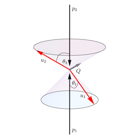
Figure 1: Example momentum parameterizations in the case of two unresolved momenta, u1u_{1} and u2u_{2}, and one reference momentum, rr, which may be either in the final state (left), or in the initial state (right, with r=p1r=p_{1}). The angles θ1\theta_{1} and θ2\theta_{2} allow for a straightforward parameterization of the collinear limits with respect to the reference momentum. QQ is the total momentum of the remaining final-state particles, while p1p_{1} and p2p_{2} are the initial-state momenta.

The resolved and unresolved parton momenta read

rμ=r0​r^μ=r0​(1𝒓^),u1μ=u10​u^1μ=u10​(1𝒖^𝟏),u2μ=u20​u^2μ=u20​(1𝒖^𝟐),r^{\mu}=r^{0}\,\hat{r}^{\mu}=r^{0}\begin{pmatrix}1\\ \bm{\hat{r}}\end{pmatrix}\;,\quad u_{1}^{\mu}=u_{1}^{0}\,\hat{u}_{1}^{\mu}=u_{1}^{0}\begin{pmatrix}1\\ \bm{\hat{u}_{1}}\end{pmatrix}\;,\quad u_{2}^{\mu}=u_{2}^{0}\,\hat{u}_{2}^{\mu}=u_{2}^{0}\begin{pmatrix}1\\ \bm{\hat{u}_{2}}\end{pmatrix}\;, (36)

with the angular parameterization (see Fig. 1)

𝒓^\displaystyle\bm{\hat{r}} =𝒏^(3−2​ϵ)​(α1,α2,…),\displaystyle=\bm{\hat{n}}^{(3-2\epsilon)}(\alpha_{1},\alpha_{2},\dots)\;,
𝒖^𝟏\displaystyle\bm{\hat{u}_{1}} =𝑹1(3−2​ϵ)​(α1,α2,…)​𝒏^(3−2​ϵ)​(θ1,ϕ1,ρ1,ρ2,…),\displaystyle=\bm{R}^{(3-2\epsilon)}_{1}(\alpha_{1},\alpha_{2},\dots)\bm{\hat{n}}^{(3-2\epsilon)}(\theta_{1},\phi_{1},\rho_{1},\rho_{2},\dots)\;,
𝒖^𝟐\displaystyle\bm{\hat{u}_{2}} =𝑹1(3−2​ϵ)​(α1,α2,…)​𝑹2(3−2​ϵ)​(ϕ1,ρ1,ρ2,…)​𝒏^(3−2​ϵ)​(θ2,ϕ2,σ1,σ2,…).\displaystyle=\bm{R}^{(3-2\epsilon)}_{1}(\alpha_{1},\alpha_{2},\dots)\bm{R}^{(3-2\epsilon)}_{2}(\phi_{1},\rho_{1},\rho_{2},\dots)\bm{\hat{n}}^{(3-2\epsilon)}(\theta_{2},\phi_{2},\sigma_{1},\sigma_{2},\dots)\;. (37)

In the case of an initial state reference momentum, the phase space is

∫d​𝚽n+2=∫d​𝚽unresolved​∫d​𝚽n​(p1+p2−u1−u2),\int\mathrm{d}\bm{\Phi}_{n+2}=\int\mathrm{d}\bm{\Phi}_{\text{unresolved}}\int\mathrm{d}\bm{\Phi}_{n}(p_{1}+p_{2}-u_{1}-u_{2})\;, (38)

while for a final state reference momentum

∫d​𝚽n+2=(μR2​eγE4​π)ϵ​∫𝒮12−2​ϵd​𝛀​(α1,α2,…)​∫d​𝚽unresolved​∫0rmax0d​r0​(r0)1−2​ϵ2​(2​π)3−2​ϵ​∫d​𝚽n−1​(p1+p2−r−u1−u2),\int\mathrm{d}\bm{\Phi}_{n+2}=\Biggl(\frac{\mu_{R}^{2}e^{\gamma_{\rm{E}}}}{4\pi}\Biggr)^{\epsilon}\int_{\mathcal{S}^{2-2\epsilon}_{1}}\mathrm{d}\bm{\Omega}(\alpha_{1},\alpha_{2},\dots)\int\mathrm{d}\bm{\Phi}_{\text{unresolved}}\int_{0}^{r_{\mathrm{max}}^{0}}\frac{\mathrm{d}r^{0}\,(r^{0})^{1-2\epsilon}}{2(2\pi)^{3-2\epsilon}}\int\mathrm{d}\bm{\Phi}_{n-1}(p_{1}+p_{2}-r-u_{1}-u_{2})\;, (39)

where

rmax0=s^​(Emax−u10−u20)+u1⋅u2s^−r^⋅(u1+u2),r_{\mathrm{max}}^{0}=\frac{\sqrt{\hat{s}}\left(E_{\mathrm{max}}-u_{1}^{0}-u_{2}^{0}\right)+u_{1}\cdot u_{2}}{\sqrt{\hat{s}}-\hat{r}\cdot\left(u_{1}+u_{2}\right)}\;, (40)

and in the particular case n=2n=2

∫0rmax0d​r0​(r0)1−2​ϵ2​(2​π)3−2​ϵ​∫d​𝚽1​(p1+p2−r−u1−u2)=(rmax0)1−2​ϵ4​(2​π)2−2​ϵ​1s^−r^⋅(u1+u2).\int_{0}^{r_{\mathrm{max}}^{0}}\frac{\mathrm{d}r^{0}\,(r^{0})^{1-2\epsilon}}{2(2\pi)^{3-2\epsilon}}\int\mathrm{d}\bm{\Phi}_{1}(p_{1}+p_{2}-r-u_{1}-u_{2})=\frac{(r_{\mathrm{max}}^{0})^{1-2\epsilon}}{4(2\pi)^{2-2\epsilon}}\frac{1}{\sqrt{\hat{s}}-\hat{r}\cdot\left(u_{1}+u_{2}\right)}\;. (41)
Figure 2: Decomposition tree of the triple-collinear sector unresolved phase space. Starting at the root with ηi=η^i\eta_{i}=\hat{\eta}_{i}, ξi=ξ^i\xi_{i}=\hat{\xi}_{i}, substitutions are performed at four levels corresponding to the factorization of the soft (I), collinear (II and III) and soft-collinear (IV) limits. The omitted right branch of the tree corresponds to a different ordering of the energies of the unresolved partons, and can be obtained by renaming the indices of the variables, 1↔21\leftrightarrow 2. The function ξ2​max\xi_{2\,\mathrm{max}} is defined in Eq. (45).

The parameters u1,20,θ1,2u_{1,2}^{0},\theta_{1,2}, and ϕ2\phi_{2} of the unresolved momenta are replaced by ξ^1,2,η^1,2\hat{\xi}_{1,2},\hat{\eta}_{1,2}, and ζ\zeta

u10=Emaxξ^1,u20=Emaxξ^2,cosθ1=1−2η^1,cosθ2=1−2η^2,cosϕ2=1−2​η3−(1−2​η^1)​(1−2​η^2)4​(1−η^1)​η^1​(1−η^2)​η^2,η3=u^1⋅u^22=1−cos⁡θ122=(η^1−η^2)2η^1+η^2−2​η^1​η^2−2​(1−2​ζ)​η^1​(1−η^1)​η^2​(1−η^2).\begin{gathered}u_{1}^{0}=E_{\mathrm{max}}\,\hat{\xi}_{1}\;,\quad u_{2}^{0}=E_{\mathrm{max}}\,\hat{\xi}_{2}\;,\\[5.69046pt] \cos\theta_{1}=1-2\hat{\eta}_{1}\;,\quad\cos\theta_{2}=1-2\hat{\eta}_{2}\;,\quad\cos\phi_{2}=\frac{1-2\eta_{3}-(1-2\hat{\eta}_{1})(1-2\hat{\eta}_{2})}{4\sqrt{(1-\hat{\eta}_{1})\hat{\eta}_{1}(1-\hat{\eta}_{2})\hat{\eta}_{2}}}\;,\\[5.69046pt] \eta_{3}=\frac{\hat{u}_{1}\cdot\hat{u}_{2}}{2}=\frac{1-\cos\theta_{12}}{2}=\frac{(\hat{\eta}_{1}-\hat{\eta}_{2})^{2}}{\hat{\eta}_{1}+\hat{\eta}_{2}-2\hat{\eta}_{1}\hat{\eta}_{2}-2(1-2\zeta)\sqrt{\hat{\eta}_{1}(1-\hat{\eta}_{1})\hat{\eta}_{2}(1-\hat{\eta}_{2})}}\;.\end{gathered} (42)

The unresolved phase space is split according to the ordering of the energies of the unresolved partons

∫d​𝚽unresolved=∫d​𝚽unresolved​(θ⁡(u10−u20)+θ⁡(u20−u10)).\int\mathrm{d}\bm{\Phi}_{\text{unresolved}}=\int\mathrm{d}\bm{\Phi}_{\text{unresolved}}\,\Big(\theta(u_{1}^{0}-u_{2}^{0})+\theta(u_{2}^{0}-u_{1}^{0})\Big)\;. (43)

Each of the two resulting contributions is further decomposed according to Fig. 2 into five sectors

∫d​𝚽unresolved​θ​(u10−u20)=(μR2​eγE4​π)2​ϵ​∫𝒮12−2​ϵd​𝛀​(θ1,ϕ1,ρ1,…)​∫𝒮12−2​ϵd​𝛀​(θ2,ϕ2,σ1,σ2,…)​∫0umax0d​u10​(u10)1−2​ϵ2​(2​π)3−2​ϵ​∫0u2​max0d​u20​(u20)1−2​ϵ2​(2​π)3−2​ϵ​θ​(u10−u20)=Emax4(2​π)6​(π​μR2​eγE8​Emax2)2​ϵ​∫𝒮11−2​ϵd​𝛀​(ϕ1,ρ1,…)​∫𝒮1−2​ϵd​𝛀​(σ1,σ2,…)​∫01d​ζ​(ζ⁡(1−ζ))−12−ϵ​⨌01d​η1​d​η2​d​ξ1​d​ξ2​∑i=15μ𝒮i,\!\!\!\!\!\!\int\mathrm{d}\bm{\Phi}_{\text{unresolved}}\,\theta(u_{1}^{0}-u_{2}^{0})=\\ \Biggl(\frac{\mu_{R}^{2}e^{\gamma_{\rm{E}}}}{4\pi}\Biggr)^{2\epsilon}\int_{\mathcal{S}^{2-2\epsilon}_{1}}\mathrm{d}\bm{\Omega}(\theta_{1},\phi_{1},\rho_{1},\dots)\int_{\mathcal{S}^{2-2\epsilon}_{1}}\mathrm{d}\bm{\Omega}(\theta_{2},\phi_{2},\sigma_{1},\sigma_{2},\dots)\int_{0}^{u^{0}_{\mathrm{max}}}\frac{\mathrm{d}u_{1}^{0}\,(u_{1}^{0})^{1-2\epsilon}}{2(2\pi)^{3-2\epsilon}}\int_{0}^{u^{0}_{2\,\mathrm{max}}}\frac{\mathrm{d}u_{2}^{0}\,(u_{2}^{0})^{1-2\epsilon}}{2(2\pi)^{3-2\epsilon}}\,\theta\big(u_{1}^{0}-u_{2}^{0}\big)\,=\\ \frac{E_{\mathrm{max}}^{4}}{(2\pi)^{6}}\bigg(\frac{\pi\mu_{R}^{2}e^{\gamma_{\rm{E}}}}{8E_{\mathrm{max}}^{2}}\bigg)^{2\epsilon}\int_{\mathcal{S}^{1-2\epsilon}_{1}}\mathrm{d}\bm{\Omega}(\phi_{1},\rho_{1},\dots)\int_{\mathcal{S}^{-2\epsilon}_{1}}\mathrm{d}\bm{\Omega}(\sigma_{1},\sigma_{2},\dots)\int_{0}^{1}\mathrm{d}\zeta\,\Big(\zeta\big(1-\zeta\big)\Big)^{-\frac{1}{2}-\epsilon}\iiiint_{0}^{1}\mathrm{d}\eta_{1}\mathrm{d}\eta_{2}\mathrm{d}\xi_{1}\mathrm{d}\xi_{2}\sum_{i=1}^{5}\mu_{\mathcal{S}_{i}}\;, (44)

where η1,2,ξ1,2\eta_{1,2},\xi_{1,2} parameterize η^1,2,ξ^1,2\hat{\eta}_{1,2},\hat{\xi}_{1,2} as in Tab. 1, while μ𝒮i\mu_{\mathcal{S}_{i}} can be found in Tab. 2, with

ξ2​max=min⁡[1,1ξ^1​1−ξ^11−2​Emaxs^​ξ^1​η3],η31​(η1,η2)=η3η1|η^1=η1η^2=η1​η2/2=(2−η2)22​(2+η2​(1−2​η1)−2​(1−2​ζ)​η2​(1−η1)​(2−η1​η2)),η32​(η1,η2)=η3η1​η22|η^1=η1η^2=η1​(2−η2)/2=12​(2+(1−2​η1)​(2−η2)−2​(1−2​ζ)​(1−η1)​(2−η2)​(2−η1​(2−η2))).\begin{gathered}\xi_{2\,\mathrm{max}}=\min\left[1,\,\frac{1}{\hat{\xi}_{1}}\frac{1-\hat{\xi}_{1}}{1-\frac{2E_{\mathrm{max}}}{\sqrt{\hat{s}}}\,\hat{\xi}_{1}\,\eta_{3}}\right]\;,\\[5.69046pt] \eta_{31}(\eta_{1},\eta_{2})=\left.\frac{\eta_{3}}{\eta_{1}}\right|_{\begin{subarray}{l}\hat{\eta}_{1}=\eta_{1}\\ \hat{\eta}_{2}=\eta_{1}\eta_{2}/2\end{subarray}}=\frac{(2-\eta_{2})^{2}}{2\left(2+\eta_{2}(1-2\eta_{1})-2(1-2\zeta)\sqrt{\eta_{2}(1-\eta_{1})(2-\eta_{1}\eta_{2})}\right)}\;,\\[5.69046pt] \eta_{32}(\eta_{1},\eta_{2})=\left.\frac{\eta_{3}}{\eta_{1}\eta_{2}^{2}}\right|_{\begin{subarray}{l}\hat{\eta}_{1}=\eta_{1}\\ \hat{\eta}_{2}=\eta_{1}(2-\eta_{2})/2\end{subarray}}=\frac{1}{2\left(2+(1-2\eta_{1})(2-\eta_{2})-2(1-2\zeta)\sqrt{(1-\eta_{1})(2-\eta_{2})(2-\eta_{1}(2-\eta_{2}))}\right)}\;.\end{gathered} (45)

The essential property of these functions is that they do not vanish in any of the singular limits of amplitudes indicated by the vanishing of any of η1,2,ξ1,2\eta_{1,2},\xi_{1,2}.

𝒮1{\cal S}_{1} 𝒮2{\cal S}_{2} 𝒮3{\cal S}_{3} 𝒮4{\cal S}_{4} 𝒮5{\cal S}_{5}
η^1\hat{\eta}_{1} η1\eta_{1} 12​η1​η2\frac{1}{2}\eta_{1}\eta_{2} 12​η1​η2​ξ2\frac{1}{2}\eta_{1}\eta_{2}\xi_{2} η1\eta_{1} 12​(2−η1)​η2\frac{1}{2}(2-\eta_{1})\eta_{2}
η^2\hat{\eta}_{2} 12​η1​η2\frac{1}{2}\eta_{1}\eta_{2} η2\eta_{2} η2\eta_{2} 12​η1​(2−η2)\frac{1}{2}\eta_{1}(2-\eta_{2}) η2\eta_{2}
ξ^1\hat{\xi}_{1} ξ1\xi_{1} ξ1\xi_{1} ξ1\xi_{1} ξ1\xi_{1} ξ1\xi_{1}
ξ^2\hat{\xi}_{2} ξ1​ξ2​ξ2​max\xi_{1}\xi_{2}\xi_{2\,\mathrm{max}} η1​ξ1​ξ2​ξ2​max\eta_{1}\xi_{1}\xi_{2}\xi_{2\,\mathrm{max}} ξ1​ξ2​ξ2​max\xi_{1}\xi_{2}\xi_{2\,\mathrm{max}} ξ1​ξ2​ξ2​max\xi_{1}\xi_{2}\xi_{2\,\mathrm{max}} ξ1​ξ2​ξ2​max\xi_{1}\xi_{2}\xi_{2\,\mathrm{max}}
Table 1: Original kinematic variables of the triple-collinear sector parameterization, η^1,η^2,ξ^1,ξ^2\hat{\eta}_{1},\hat{\eta}_{2},\hat{\xi}_{1},\hat{\xi}_{2}, expressed through the sector variables, η1,η2,ξ1,ξ2\eta_{1},\eta_{2},\xi_{1},\xi_{2}, of the five sectors, 𝒮1,…,𝒮5\mathcal{S}_{1},\dots,\mathcal{S}_{5}, defined in Fig. 2. The function ξ2​max\xi_{2\,\mathrm{max}} is defined in Eq. (45).
μ𝒮i\mu_{\mathcal{S}_{i}}
𝒮1\mathcal{S}_{1} η11−2​ϵ​η2−ϵ​ξ13−4​ϵ​ξ21−2​ϵ​((1−η1)​(2−η1​η2))−ϵ​(η31​(η1,η2)2−η2)1−2​ϵ​ξ2​max 2−2​ϵ\displaystyle\eta_{1}^{1-2\epsilon}\eta_{2}^{-\epsilon}\xi_{1}^{3-4\epsilon}\xi_{2}^{1-2\epsilon}\left((1-\eta_{1})(2-\eta_{1}\eta_{2})\right)^{-\epsilon}\left(\frac{\eta_{31}(\eta_{1},\eta_{2})}{2-\eta_{2}}\right)^{1-2\epsilon}\xi_{2\,\mathrm{max}}^{\;2-2\epsilon}
𝒮2\mathcal{S}_{2} η12−3​ϵ​η21−2​ϵ​ξ13−4​ϵ​ξ21−2​ϵ​((1−η2)​(2−η1​η2))−ϵ​(η31​(η2,η1)2−η1)1−2​ϵ​ξ2​max 2−2​ϵ\displaystyle\eta_{1}^{2-3\epsilon}\eta_{2}^{1-2\epsilon}\xi_{1}^{3-4\epsilon}\xi_{2}^{1-2\epsilon}\left((1-\eta_{2})(2-\eta_{1}\eta_{2})\right)^{-\epsilon}\left(\frac{\eta_{31}(\eta_{2},\eta_{1})}{2-\eta_{1}}\right)^{1-2\epsilon}\xi_{2\,\mathrm{max}}^{\;2-2\epsilon}
𝒮3\mathcal{S}_{3} η1−ϵ​η21−2​ϵ​ξ13−4​ϵ​ξ22−3​ϵ​((1−η2)​(2−η1​η2​ξ2))−ϵ​(η31​(η2,η1​ξ2)2−η1​ξ2)1−2​ϵ​ξ2​max 2−2​ϵ\displaystyle\eta_{1}^{-\epsilon}\eta_{2}^{1-2\epsilon}\xi_{1}^{3-4\epsilon}\xi_{2}^{2-3\epsilon}\left((1-\eta_{2})(2-\eta_{1}\eta_{2}\xi_{2})\right)^{-\epsilon}\left(\frac{\eta_{31}(\eta_{2},\eta_{1}\xi_{2})}{2-\eta_{1}\xi_{2}}\right)^{1-2\epsilon}\xi_{2\,\mathrm{max}}^{\;2-2\epsilon}
𝒮4\mathcal{S}_{4} η11−2​ϵ​η21−2​ϵ​ξ13−4​ϵ​ξ21−2​ϵ​((1−η1)​(2−η2)​(2−η1​(2−η2)))−ϵ​η321−2​ϵ​(η1,η2)​ξ2​max 2−2​ϵ\eta_{1}^{1-2\epsilon}\eta_{2}^{1-2\epsilon}\xi_{1}^{3-4\epsilon}\xi_{2}^{1-2\epsilon}\left((1-\eta_{1})(2-\eta_{2})(2-\eta_{1}(2-\eta_{2}))\right)^{-\epsilon}\eta_{32}^{1-2\epsilon}(\eta_{1},\eta_{2})\,\xi_{2\,\mathrm{max}}^{\;2-2\epsilon}
𝒮5\mathcal{S}_{5} η11−2​ϵ​η21−2​ϵ​ξ13−4​ϵ​ξ21−2​ϵ​((1−η2)​(2−η1)​(2−η2​(2−η1)))−ϵ​η321−2​ϵ​(η2,η1)​ξ2​max 2−2​ϵ\eta_{1}^{1-2\epsilon}\eta_{2}^{1-2\epsilon}\xi_{1}^{3-4\epsilon}\xi_{2}^{1-2\epsilon}\left((1-\eta_{2})(2-\eta_{1})(2-\eta_{2}(2-\eta_{1}))\right)^{-\epsilon}\eta_{32}^{1-2\epsilon}(\eta_{2},\eta_{1})\,\xi_{2\,\mathrm{max}}^{\;2-2\epsilon}
Table 2: Integration measures, μ𝒮i\mu_{\mathcal{S}_{i}}, of the five sectors 𝒮1,…,𝒮5\mathcal{S}_{1},\dots,\mathcal{S}_{5}, of the triple-collinear sector parameterization. The functions η31,η32\eta_{31},\eta_{32} and ξ2​max\xi_{2\,\mathrm{max}} are defined in Eq. (45).

The behavior of amplitudes in collinear limits is characterized by the transverse vectors

ui⟂μ=(0𝒖^𝒊⟂),i=1,2,3,u_{i\perp}^{\mu}=\begin{pmatrix}0\\ \bm{\hat{u}_{i\perp}}\end{pmatrix}\;,\quad i=1,2,3\;, (46)

with

𝒖^𝟏⟂=limθ1→0𝒖^𝟏−𝒓^∥𝒖^𝟏−𝒓^∥\displaystyle\bm{\hat{u}_{1\perp}}=\lim_{\theta_{1}\to 0}\frac{\bm{\hat{u}_{1}}-\bm{\hat{r}}}{\lVert\bm{\hat{u}_{1}}-\bm{\hat{r}}\rVert} =∂𝒖^𝟏∂θ1|θ1=0=𝑹^1(3−2​ϵ)​(α1,α2,…)​𝒏^(3−2​ϵ)​(π2,ϕ1,ρ1,ρ2,…),\displaystyle=\left.\frac{\partial\bm{\hat{u}_{1}}}{\partial\theta_{1}}\right|_{\theta_{1}=0}=\bm{\hat{R}}^{(3-2\epsilon)}_{1}(\alpha_{1},\alpha_{2},\dots)\bm{\hat{n}}^{(3-2\epsilon)}\left(\frac{\pi}{2},\phi_{1},\rho_{1},\rho_{2},\dots\right)\;, (47)
𝒖^𝟐⟂=limθ2→0𝒖^𝟐−𝒓^∥𝒖^𝟐−𝒓^∥\displaystyle\bm{\hat{u}_{2\perp}}=\lim_{\theta_{2}\to 0}\frac{\bm{\hat{u}_{2}}-\bm{\hat{r}}}{\lVert\bm{\hat{u}_{2}}-\bm{\hat{r}}\rVert} =∂𝒖^𝟐∂θ2|θ2=0=𝑹^1(3−2​ϵ)​(α1,α2,…)​𝑹^2(3−2​ϵ)​(ϕ1,ρ1,ρ2,…)​𝒏^(3−2​ϵ)​(π2,ϕ2,σ1,σ2,…).\displaystyle=\left.\frac{\partial\bm{\hat{u}_{2}}}{\partial\theta_{2}}\right|_{\theta_{2}=0}=\bm{\hat{R}}^{(3-2\epsilon)}_{1}(\alpha_{1},\alpha_{2},\dots)\bm{\hat{R}}^{(3-2\epsilon)}_{2}(\phi_{1},\rho_{1},\rho_{2},\dots)\bm{\hat{n}}^{(3-2\epsilon)}\left(\frac{\pi}{2},\phi_{2},\sigma_{1},\sigma_{2},\dots\right)\;. (48)

In order to determine the third transverse vector, let us consider a general parameterization

ϕ2=ϕ2(θ1,θ2,ζ)=ϕ2(θ2,θ1,ζ),ϕ2(θ1,θ1,ζ)=0,ϕ2​(θ1,θ2,ζ)=∂θ2+ϕ2​(θ1,ζ)​|θ2−θ1|+𝒪⁡((θ2−θ1)2),∂θ2+ϕ2​(θ1,ζ)=limθ2→θ1+ϕ2​(θ1,θ2,ζ)−ϕ2​(θ1,θ1,ζ)θ2−θ1.\begin{gathered}\phi_{2}=\phi_{2}(\theta_{1},\theta_{2},\zeta)=\phi_{2}(\theta_{2},\theta_{1},\zeta)\;,\quad\phi_{2}(\theta_{1},\theta_{1},\zeta)=0\;,\\[8.5359pt] \phi_{2}(\theta_{1},\theta_{2},\zeta)=\partial^{+}_{\theta_{2}}\phi_{2}(\theta_{1},\zeta)\,\big|\theta_{2}-\theta_{1}\big|+\mathcal{O}\big((\theta_{2}-\theta_{1})^{2}\big)\;,\\[5.69046pt] \partial^{+}_{\theta_{2}}\phi_{2}(\theta_{1},\zeta)=\lim_{\theta_{2}\to\theta_{1}^{+}}\frac{\phi_{2}(\theta_{1},\theta_{2},\zeta)-\phi_{2}(\theta_{1},\theta_{1},\zeta)}{\theta_{2}-\theta_{1}}\;.\end{gathered} (49)

We then have

𝒖^𝟑⟂±=limθ2→θ1±𝒖^𝟐−𝒖^𝟏∥𝒖^𝟐−𝒖^𝟏∥=±𝒩3⟂(θ1,ζ)limθ2→θ1±𝒖^𝟐−𝒖^𝟏θ2−θ1=±𝒩3⟂(θ1,ζ)𝑹^(3−2​ϵ)1(α1,α2,…)𝑹^(3−2​ϵ)1(θ1,ϕ1,ρ1,ρ2,…)×(𝒏^(3−2​ϵ)​(π2,0,0,…)±sin⁡θ1​∂θ2+ϕ2​(θ1,ζ)​𝒏^(3−2​ϵ)​(π2,π2,σ1,σ2,…)),\bm{\hat{u}_{3\perp}}^{\pm}=\lim_{\theta_{2}\to\theta_{1}^{\pm}}\frac{\bm{\hat{u}_{2}}-\bm{\hat{u}_{1}}}{\lVert\bm{\hat{u}_{2}}-\bm{\hat{u}_{1}}\rVert}=\pm\mathcal{N}_{3\perp}(\theta_{1},\zeta)\lim_{\theta_{2}\to\theta_{1}^{\pm}}\frac{\bm{\hat{u}_{2}}-\bm{\hat{u}_{1}}}{\theta_{2}-\theta_{1}}=\pm\mathcal{N}_{3\perp}(\theta_{1},\zeta)\,\bm{\hat{R}}^{(3-2\epsilon)}_{1}(\alpha_{1},\alpha_{2},\dots)\bm{\hat{R}}^{(3-2\epsilon)}_{1}(\theta_{1},\phi_{1},\rho_{1},\rho_{2},\dots)\\ \times\left(\bm{\hat{n}}^{(3-2\epsilon)}\left(\frac{\pi}{2},0,0,\dots\right)\pm\sin\theta_{1}\,\partial^{+}_{\theta_{2}}\phi_{2}(\theta_{1},\zeta)\,\bm{\hat{n}}^{(3-2\epsilon)}\left(\frac{\pi}{2},\frac{\pi}{2},\sigma_{1},\sigma_{2},\dots\right)\right)\;, (50)

where 𝒩3⟂​(θ1,ζ)\mathcal{N}_{3\perp}(\theta_{1},\zeta) is the positive normalization factor

𝒩3⟂​(θ1,ζ)=[1+(sin⁡θ1​∂θ2+ϕ2​(θ1,ζ))2]−12.\mathcal{N}_{3\perp}(\theta_{1},\zeta)=\left[1+\left(\sin\theta_{1}\,\partial^{+}_{\theta_{2}}\phi_{2}(\theta_{1},\zeta)\right)^{2}\right]^{-\frac{1}{2}}\;. (51)

The transverse vector can be reexpressed as

𝒖^𝟑⟂±=𝑹^1(3−2​ϵ)​(α1,α2,…)​𝑹^1(3−2​ϵ)​(θ1,ϕ1,ρ1,ρ2,…)​𝒏^(3−2​ϵ)​(π2,ϕ~2±,σ1,σ2,…),\bm{\hat{u}_{3\perp}}^{\pm}=\bm{\hat{R}}^{(3-2\epsilon)}_{1}(\alpha_{1},\alpha_{2},\dots)\bm{\hat{R}}^{(3-2\epsilon)}_{1}(\theta_{1},\phi_{1},\rho_{1},\rho_{2},\dots)\bm{\hat{n}}^{(3-2\epsilon)}\left(\frac{\pi}{2},\tilde{\phi}_{2}^{\pm},\sigma_{1},\sigma_{2},\dots\right)\;, (52)

with

tanϕ~2±(θ1,ζ)=±sinθ1∂θ2+ϕ2(θ1,ζ),ϕ~2+∈[0,π2[,ϕ~2−∈[π2,π[.\tan\tilde{\phi}^{\pm}_{2}(\theta_{1},\zeta)=\pm\sin\theta_{1}\,\partial^{+}_{\theta_{2}}\phi_{2}(\theta_{1},\zeta)\;,\quad\tilde{\phi}^{+}_{2}\in\left[0,\frac{\pi}{2}\right[\;,\quad\tilde{\phi}^{-}_{2}\in\left[\frac{\pi}{2},\pi\right[\;. (53)

For our particular choice of the dependence of ϕ2\phi_{2} on ζ\zeta, Eq. (42), there is

cos⁡ϕ~2±=±ζ,sin⁡ϕ~2±=1−ζ.\cos\tilde{\phi}^{\pm}_{2}=\pm\sqrt{\zeta}\;,\quad\sin\tilde{\phi}^{\pm}_{2}=\sqrt{1-\zeta}\;. (54)

4.3 Double-collinear sector parameterization: two reference momenta, two unresolved momenta

4.3.1 General case with n>nf​rn>n_{fr}
Refer to caption
Refer to caption
Figure 3: Example momentum parameterizations in the case of two unresolved momenta, u1u_{1} and u2u_{2}, and two reference momenta, r1r_{1} and r2r_{2}. The left picture shows a case with initial state reference momenta with r1=p2r_{1}=p_{2} and r2=p1r_{2}=p_{1}, while the right picture shows a mixed case with one final state reference momentum, r1r_{1}, and one initial state reference momentum, r2=p1r_{2}=p_{1}. The angles θ1\theta_{1} and θ2\theta_{2} allow for a straightforward parameterization of the collinear limits with respect to the reference momenta. QQ is the total momentum of the remaining final-state particles, while p1p_{1} and p2p_{2} are the initial-state momenta.

The resolved and unresolved parton momenta read

r1μ=r10​r^1μ=r10​(1𝒓^𝟏),r2μ=r20​r^2μ=r20​(1𝒓^𝟐),u1μ=u10​u^1μ=u10​(1𝒖^𝟏),u2μ=u20​u^2μ=u20​(1𝒖^𝟐),r_{1}^{\mu}=r_{1}^{0}\,\hat{r}_{1}^{\mu}=r_{1}^{0}\begin{pmatrix}1\\ \bm{\hat{r}_{1}}\end{pmatrix}\;,\quad r_{2}^{\mu}=r_{2}^{0}\,\hat{r}_{2}^{\mu}=r_{2}^{0}\begin{pmatrix}1\\ \bm{\hat{r}_{2}}\end{pmatrix}\;,\quad u_{1}^{\mu}=u_{1}^{0}\,\hat{u}_{1}^{\mu}=u_{1}^{0}\begin{pmatrix}1\\ \bm{\hat{u}_{1}}\end{pmatrix}\;,\quad u_{2}^{\mu}=u_{2}^{0}\,\hat{u}_{2}^{\mu}=u_{2}^{0}\begin{pmatrix}1\\ \bm{\hat{u}_{2}}\end{pmatrix}\;, (55)

with the angular parameterization (see Fig. 3)

𝒓^𝟏\displaystyle\bm{\hat{r}_{1}} =𝒏^(3−2​ϵ)​(α1,α2,…),\displaystyle=\bm{\hat{n}}^{(3-2\epsilon)}(\alpha_{1},\alpha_{2},\dots)\;,
𝒓^𝟐\displaystyle\bm{\hat{r}_{2}} =𝒏^(3−2​ϵ)​(β1,β2,…),\displaystyle=\bm{\hat{n}}^{(3-2\epsilon)}(\beta_{1},\beta_{2},\dots)\;,
𝒖^𝟏\displaystyle\bm{\hat{u}_{1}} =𝑹1(3−2​ϵ)​(α1,α2,…)​𝒏^(3−2​ϵ)​(θ1,ϕ1,ρ1,ρ2,…),\displaystyle=\bm{R}^{(3-2\epsilon)}_{1}(\alpha_{1},\alpha_{2},\dots)\bm{\hat{n}}^{(3-2\epsilon)}(\theta_{1},\phi_{1},\rho_{1},\rho_{2},\dots)\;,
𝒖^𝟐\displaystyle\bm{\hat{u}_{2}} =𝑹1(3−2​ϵ)​(β1,β2,…)​𝑹4(3−2​ϵ)​(ρ2,ρ3,…)​𝒏^(3−2​ϵ)​(θ2,ϕ2,σ1,σ2,…).\displaystyle=\bm{R}^{(3-2\epsilon)}_{1}(\beta_{1},\beta_{2},\dots)\bm{R}^{(3-2\epsilon)}_{4}(\rho_{2},\rho_{3},\dots)\bm{\hat{n}}^{(3-2\epsilon)}(\theta_{2},\phi_{2},\sigma_{1},\sigma_{2},\dots)\;. (56)

In the case of two initial state reference momenta, the phase space is

∫d​𝚽n+2=∫d​𝚽unresolved​∫d​𝚽n​(p1+p2−u1−u2),\int\mathrm{d}\bm{\Phi}_{n+2}=\int\mathrm{d}\bm{\Phi}_{\text{unresolved}}\int\mathrm{d}\bm{\Phi}_{n}(p_{1}+p_{2}-u_{1}-u_{2})\;, (57)

while for one final state (r1r_{1}) and one initial state (r2r_{2}) reference momentum

∫d​𝚽n+2=(μR2​eγE4​π)ϵ​∫𝒮12−2​ϵd​𝛀​(α1,α2,…)​∫d​𝚽unresolved​∫0rmax0d​r10​(r10)1−2​ϵ2​(2​π)3−2​ϵ​∫d​𝚽n−1​(p1+p2−r1−u1−u2),\int\mathrm{d}\bm{\Phi}_{n+2}=\Biggl(\frac{\mu_{R}^{2}e^{\gamma_{\rm{E}}}}{4\pi}\Biggr)^{\epsilon}\int_{\mathcal{S}^{2-2\epsilon}_{1}}\mathrm{d}\bm{\Omega}(\alpha_{1},\alpha_{2},\dots)\int\mathrm{d}\bm{\Phi}_{\text{unresolved}}\int_{0}^{r_{\mathrm{max}}^{0}}\frac{\mathrm{d}r_{1}^{0}\,(r_{1}^{0})^{1-2\epsilon}}{2(2\pi)^{3-2\epsilon}}\int\mathrm{d}\bm{\Phi}_{n-1}(p_{1}+p_{2}-r_{1}-u_{1}-u_{2})\;, (58)

and similarly if the rôles of r1r_{1} and r2r_{2} are reversed. For two final state reference momenta, there is

∫d​𝚽n+2=(μR2​eγE4​π)2​ϵ​∫𝒮12−2​ϵd​𝛀​(α1,α2,…)​∫𝒮12−2​ϵd​𝛀​(β1,β2,…)​∫d​𝚽unresolved×∫0rmax0d​r10​(r10)1−2​ϵ2​(2​π)3−2​ϵ​∫0r2​max0d​r20​(r20)1−2​ϵ2​(2​π)3−2​ϵ​∫d​𝚽n−2​(p1+p2−r1−r2−u1−u2).\int\mathrm{d}\bm{\Phi}_{n+2}=\Biggl(\frac{\mu_{R}^{2}e^{\gamma_{\rm{E}}}}{4\pi}\Biggr)^{2\epsilon}\int_{\mathcal{S}^{2-2\epsilon}_{1}}\mathrm{d}\bm{\Omega}(\alpha_{1},\alpha_{2},\dots)\int_{\mathcal{S}^{2-2\epsilon}_{1}}\mathrm{d}\bm{\Omega}(\beta_{1},\beta_{2},\dots)\int\mathrm{d}\bm{\Phi}_{\text{unresolved}}\\ \times\int_{0}^{r_{\mathrm{max}}^{0}}\frac{\mathrm{d}r_{1}^{0}\,(r_{1}^{0})^{1-2\epsilon}}{2(2\pi)^{3-2\epsilon}}\int_{0}^{r_{2\,\mathrm{max}}^{0}}\frac{\mathrm{d}r_{2}^{0}\,(r_{2}^{0})^{1-2\epsilon}}{2(2\pi)^{3-2\epsilon}}\int\mathrm{d}\bm{\Phi}_{n-2}(p_{1}+p_{2}-r_{1}-r_{2}-u_{1}-u_{2})\;. (59)

rmax0r_{\mathrm{max}}^{0} is defined in Eq. (40) with r^=r^1\hat{r}=\hat{r}_{1}. If the second reference momentum is in the initial state and n=2n=2, then Eq. (41) applies. Furthermore, in the case of two final state reference momenta

r2​max0=s^​(Emax−u10−u20−r10)+r1⋅(u1+u2)+u1⋅u2s^−r^2⋅(u1+u2+r1),r_{2\,\mathrm{max}}^{0}=\frac{\sqrt{\hat{s}}\left(E_{\mathrm{max}}-u_{1}^{0}-u_{2}^{0}-r_{1}^{0}\right)+r_{1}\cdot(u_{1}+u_{2})+u_{1}\cdot u_{2}}{\sqrt{\hat{s}}-\hat{r}_{2}\cdot\left(u_{1}+u_{2}+r_{1}\right)}\;, (60)

and in the particular case n=3n=3

∫0r2​max0d​r20​(r20)1−2​ϵ2​(2​π)3−2​ϵ​∫d​𝚽1​(p1+p2−u1−u2)=(r2​max0)1−2​ϵ4​(2​π)2−2​ϵ​1s^−r^2⋅(u1+u2+r1).\int_{0}^{r_{2\,\mathrm{max}}^{0}}\frac{\mathrm{d}r_{2}^{0}\,(r_{2}^{0})^{1-2\epsilon}}{2(2\pi)^{3-2\epsilon}}\int\mathrm{d}\bm{\Phi}_{1}(p_{1}+p_{2}-u_{1}-u_{2})=\frac{(r_{2\,\mathrm{max}}^{0})^{1-2\epsilon}}{4(2\pi)^{2-2\epsilon}}\frac{1}{\sqrt{\hat{s}}-\hat{r}_{2}\cdot\left(u_{1}+u_{2}+r_{1}\right)}\;. (61)

The unresolved phase space is split according to the ordering of the energies of the unresolved partons

∫d​𝚽unresolved=∫d​𝚽unresolved​(θ⁡(u10−u20)+θ⁡(u20−u10)),\int\mathrm{d}\bm{\Phi}_{\text{unresolved}}=\int\mathrm{d}\bm{\Phi}_{\text{unresolved}}\,\Big(\theta(u_{1}^{0}-u_{2}^{0})+\theta(u_{2}^{0}-u_{1}^{0})\Big)\;, (62)

with

∫d​𝚽unresolved​θ​(u10−u20)=(μR2​eγE4​π)2​ϵ​∫𝒮12−2​ϵd​𝛀​(θ1,ϕ1,ρ1,…)​∫𝒮12−2​ϵd​𝛀​(θ2,ϕ2,σ1,σ2,…)​∫0umax0d​u10​(u10)1−2​ϵ2​(2​π)3−2​ϵ​∫0u2​max0d​u20​(u20)1−2​ϵ2​(2​π)3−2​ϵ​θ​(u10−u20)=Emax4(2​π)6​(π​μR2​eγE4​Emax2)2​ϵ​∫𝒮11−2​ϵd​𝛀​(ϕ1,ρ1,…)​∫𝒮11−2​ϵd​𝛀​(ϕ2,σ1,σ2,…)×⨌01d​η1​d​η2​d​ξ1​d​ξ2​η1−ϵ​η2−ϵ​ξ13−4​ϵ​ξ21−2​ϵ​((1−η1)​(1−η2))−ϵ​ξ2​max2−2​ϵ,\!\!\!\!\!\!\int\mathrm{d}\bm{\Phi}_{\text{unresolved}}\,\theta(u_{1}^{0}-u_{2}^{0})=\\ \Biggl(\frac{\mu_{R}^{2}e^{\gamma_{\rm{E}}}}{4\pi}\Biggr)^{2\epsilon}\int_{\mathcal{S}^{2-2\epsilon}_{1}}\mathrm{d}\bm{\Omega}(\theta_{1},\phi_{1},\rho_{1},\dots)\int_{\mathcal{S}^{2-2\epsilon}_{1}}\mathrm{d}\bm{\Omega}(\theta_{2},\phi_{2},\sigma_{1},\sigma_{2},\dots)\int_{0}^{u^{0}_{\mathrm{max}}}\frac{\mathrm{d}u_{1}^{0}\,(u_{1}^{0})^{1-2\epsilon}}{2(2\pi)^{3-2\epsilon}}\int_{0}^{u^{0}_{2\,\mathrm{max}}}\frac{\mathrm{d}u_{2}^{0}\,(u_{2}^{0})^{1-2\epsilon}}{2(2\pi)^{3-2\epsilon}}\,\theta\big(u_{1}^{0}-u_{2}^{0}\big)\,=\\ \frac{E_{\mathrm{max}}^{4}}{(2\pi)^{6}}\bigg(\frac{\pi\mu_{R}^{2}e^{\gamma_{\rm{E}}}}{4E_{\mathrm{max}}^{2}}\bigg)^{2\epsilon}\int_{\mathcal{S}^{1-2\epsilon}_{1}}\mathrm{d}\bm{\Omega}(\phi_{1},\rho_{1},\dots)\int_{\mathcal{S}^{1-2\epsilon}_{1}}\mathrm{d}\bm{\Omega}(\phi_{2},\sigma_{1},\sigma_{2},\dots)\\ \times\iiiint_{0}^{1}\mathrm{d}\eta_{1}\mathrm{d}\eta_{2}\mathrm{d}\xi_{1}\mathrm{d}\xi_{2}\,\eta_{1}^{-\epsilon}\eta_{2}^{-\epsilon}\xi_{1}^{3-4\epsilon}\xi_{2}^{1-2\epsilon}\Big(\big(1-\eta_{1}\big)\big(1-\eta_{2}\big)\Big)^{-\epsilon}\xi_{2\,\mathrm{max}}^{2-2\epsilon}\;, (63)

where

u10=Emaxξ1,u20=Emaxξ1ξ2ξ2​max,ξ2​max=min[1,1ξ11−ξ11−Emaxs^​ξ1​u^1⋅u^2],cosθ1=1−2η1,cosθ2=1−2η2.\begin{gathered}u_{1}^{0}=E_{\mathrm{max}}\,\xi_{1}\;,\quad u_{2}^{0}=E_{\mathrm{max}}\,\xi_{1}\xi_{2}\xi_{2\,\mathrm{max}}\;,\quad\xi_{2\,\mathrm{max}}=\min\left[1,\,\frac{1}{\xi_{1}}\frac{1-\xi_{1}}{1-\frac{E_{\mathrm{max}}}{\sqrt{\hat{s}}}\,\xi_{1}\,\hat{u}_{1}\cdot\hat{u}_{2}}\right]\;,\\[5.69046pt] \cos\theta_{1}=1-2\eta_{1}\;,\quad\cos\theta_{2}=1-2\eta_{2}\;.\end{gathered} (64)

Notice that if αi=βi=0\alpha_{i}=\beta_{i}=0 for i>2i>2, then u^1⋅u^2\hat{u}_{1}\cdot\hat{u}_{2} is only a function of α1,2,β1,2,θ1,2,ϕ1,2,ρ1\alpha_{1,2},\beta_{1,2},\theta_{1,2},\phi_{1,2},\rho_{1}, and σ1,2\sigma_{1,2}. This fact will be important for the four-dimensional formulation of the subtraction scheme.

The behavior of amplitudes in collinear limits is characterized by the transverse vectors

ui⟂μ=(0𝒖^𝒊⟂),i=1,2,u_{i\perp}^{\mu}=\begin{pmatrix}0\\ \bm{\hat{u}_{i\perp}}\end{pmatrix}\;,\quad i=1,2\;, (65)

with

𝒖^𝟏⟂\displaystyle\bm{\hat{u}_{1\perp}} =limθ1→0𝒖^𝟏−𝒓^𝟏∥𝒖^𝟏−𝒓^𝟏∥=∂𝒖^𝟏∂θ1|θ1=0=𝑹^1(3−2​ϵ)​(α1,α2,…)​𝒏^(3−2​ϵ)​(π2,ϕ1,ρ1,ρ2,…),\displaystyle=\lim_{\theta_{1}\to 0}\frac{\bm{\hat{u}_{1}}-\bm{\hat{r}_{1}}}{\lVert\bm{\hat{u}_{1}}-\bm{\hat{r}_{1}}\rVert}=\left.\frac{\partial\bm{\hat{u}_{1}}}{\partial\theta_{1}}\right|_{\theta_{1}=0}=\bm{\hat{R}}^{(3-2\epsilon)}_{1}(\alpha_{1},\alpha_{2},\dots)\bm{\hat{n}}^{(3-2\epsilon)}\left(\frac{\pi}{2},\phi_{1},\rho_{1},\rho_{2},\dots\right)\;, (66)
𝒖^𝟐⟂\displaystyle\bm{\hat{u}_{2\perp}} =limθ2→0𝒖^𝟐−𝒓^𝟐∥𝒖^𝟐−𝒓^𝟐∥=∂𝒖^𝟐∂θ2|θ2=0=𝑹^1(3−2​ϵ)​(β1,β2,…)​𝑹^4(3−2​ϵ)​(ρ2,ρ3,…)​𝒏^(3−2​ϵ)​(π2,ϕ2,σ1,σ2,…).\displaystyle=\lim_{\theta_{2}\to 0}\frac{\bm{\hat{u}_{2}}-\bm{\hat{r}_{2}}}{\lVert\bm{\hat{u}_{2}}-\bm{\hat{r}_{2}}\rVert}=\left.\frac{\partial\bm{\hat{u}_{2}}}{\partial\theta_{2}}\right|_{\theta_{2}=0}=\bm{\hat{R}}^{(3-2\epsilon)}_{1}(\beta_{1},\beta_{2},\dots)\bm{\hat{R}}^{(3-2\epsilon)}_{4}(\rho_{2},\rho_{3},\dots)\bm{\hat{n}}^{(3-2\epsilon)}\left(\frac{\pi}{2},\phi_{2},\sigma_{1},\sigma_{2},\dots\right)\;. (67)

4.3.2 Special case with n=nu=nf​r=2n=n_{u}=n_{fr}=2

Refer to caption
Figure 4: Parameterization of a fully massless four-particle phase space (left), where two of the final states are used as reference vectors, r1r_{1} and r2r_{2}, while the other two, u1u_{1} and u2u_{2}, are considered to be unresolved. p1p_{1} and p2p_{2} are initial state momenta, while rr is a reference vector equal to the sum of one reference and one unresolved momentum, r=r1+u1r=r_{1}+u_{1}. If the parameters of one of the unresolved momenta are specified, then the available range of parameters of the other one is split into two disjunct regions (right). There are neither soft nor collinear singularities in region II.

This is a parameterization of a fully massless four-particle phase space. Unlike previous cases, it uses an auxiliary reference vector, 𝒓\bm{r}. The configuration is depicted in Fig. 4, and defines the following reference and unresolved momenta

r1μ=r10​r^1μ=r10​(1𝒓^𝟏),r2μ=r20​r^2μ=r20​(1𝒓^𝟐),u1μ=u10​u^1μ=u10​(1𝒖^𝟏),u2μ=u20​u^2μ=u20​(1𝒖^𝟐),r_{1}^{\mu}=r_{1}^{0}\,\hat{r}_{1}^{\mu}=r_{1}^{0}\begin{pmatrix}1\\ \bm{\hat{r}_{1}}\end{pmatrix}\;,\quad r_{2}^{\mu}=r_{2}^{0}\,\hat{r}_{2}^{\mu}=r_{2}^{0}\begin{pmatrix}1\\ \bm{\hat{r}_{2}}\end{pmatrix}\;,\quad u_{1}^{\mu}=u_{1}^{0}\,\hat{u}_{1}^{\mu}=u_{1}^{0}\begin{pmatrix}1\\ \bm{\hat{u}_{1}}\end{pmatrix}\;,\quad u_{2}^{\mu}=u_{2}^{0}\,\hat{u}_{2}^{\mu}=u_{2}^{0}\begin{pmatrix}1\\ \bm{\hat{u}_{2}}\end{pmatrix}\;, (68)

where

𝒓=r10​𝒓^𝟏+u10​𝒖^𝟏=−r20​𝒓^𝟐−u20​𝒖^𝟐,r=∥𝒓∥,𝒓^=𝒓r,\bm{r}=r_{1}^{0}\,\bm{\hat{r}_{1}}+u_{1}^{0}\,\bm{\hat{u}_{1}}=-r_{2}^{0}\,\bm{\hat{r}_{2}}-u_{2}^{0}\,\bm{\hat{u}_{2}}\;,\quad r=\lVert\bm{r}\rVert\;,\quad\bm{\hat{r}}=\frac{\bm{r}}{r}\;, (69)

with the angular parameterization

𝒓^\displaystyle\bm{\hat{r}} =𝒏^(3−2​ϵ)​(α1,α2,…),\displaystyle=\bm{\hat{n}}^{(3-2\epsilon)}(\alpha_{1},\alpha_{2},\dots)\;,
𝒖^𝟏\displaystyle\bm{\hat{u}_{1}} =𝑹1(3−2​ϵ)​(α1,α2,…)​𝒏^(3−2​ϵ)​(θ~1,ϕ1,ρ1,ρ2,…),\displaystyle=\bm{R}^{(3-2\epsilon)}_{1}(\alpha_{1},\alpha_{2},\dots)\bm{\hat{n}}^{(3-2\epsilon)}(\tilde{\theta}_{1},\phi_{1},\rho_{1},\rho_{2},\dots)\;,
𝒖^𝟐\displaystyle\bm{\hat{u}_{2}} =𝑹1(3−2​ϵ)​(α1,α2,…)​𝑹4(3−2​ϵ)​(ρ2,ρ3,…)​𝒏^(3−2​ϵ)​(θ~2,ϕ2,σ1,σ2,…).\displaystyle=\bm{R}^{(3-2\epsilon)}_{1}(\alpha_{1},\alpha_{2},\dots)\bm{R}^{(3-2\epsilon)}_{4}(\rho_{2},\rho_{3},\dots)\bm{\hat{n}}^{(3-2\epsilon)}(\tilde{\theta}_{2},\phi_{2},\sigma_{1},\sigma_{2},\dots)\;. (70)

We start with a general discussion of the phase space. A parameterization suitable for the derivation of the subtraction and integrated subtraction terms will be provided near the end of the section. We write

∫d​𝚽4=(μR2​eγE4​π)3​ϵ​∫𝒮12−2​ϵd​𝛀​(α1,α2,…)×∫𝒮11−2​ϵd​𝛀​(ϕ1,ρ1,…)​∫𝒮11−2​ϵd​𝛀​(ϕ2,σ1,σ2,…)×∫0∞d​u10​(u10)1−2​ϵ2​(2​π)3−2​ϵ∫−11dcosθ1(1−cos2θ1)−ϵ∫0∞d​u20​(u20)1−2​ϵ2​(2​π)3−2​ϵ∫−11dcosθ2(1−cos2θ2)−ϵ×(1−cos2⁡θ~11−cos2⁡θ1)−ϵ​(1−cos2⁡θ~21−cos2⁡θ2)−ϵ​r10​r204(2π)2−2​ϵr1+2​ϵ|r10+r20+u10cosθ1+u20cosθ2|,\begin{split}\int\mathrm{d}\bm{\Phi}_{4}&=\Biggl(\frac{\mu_{R}^{2}e^{\gamma_{\rm{E}}}}{4\pi}\Biggr)^{3\epsilon}\int_{\mathcal{S}^{2-2\epsilon}_{1}}\mathrm{d}\bm{\Omega}(\alpha_{1},\alpha_{2},\dots)\\ &\times\int_{\mathcal{S}^{1-2\epsilon}_{1}}\mathrm{d}\bm{\Omega}(\phi_{1},\rho_{1},\dots)\int_{\mathcal{S}^{1-2\epsilon}_{1}}\mathrm{d}\bm{\Omega}(\phi_{2},\sigma_{1},\sigma_{2},\dots)\\ &\times\int_{0}^{\infty}\frac{\mathrm{d}u_{1}^{0}\,(u_{1}^{0})^{1-2\epsilon}}{2(2\pi)^{3-2\epsilon}}\int_{-1}^{1}\mathrm{d}\cos\theta_{1}\,\left(1-\cos^{2}\theta_{1}\right)^{-\epsilon}\int_{0}^{\infty}\frac{\mathrm{d}u_{2}^{0}(u_{2}^{0})^{1-2\epsilon}}{2(2\pi)^{3-2\epsilon}}\int_{-1}^{1}\mathrm{d}\cos\theta_{2}\,\left(1-\cos^{2}\theta_{2}\right)^{-\epsilon}\\ &\times\left(\frac{1-\cos^{2}\tilde{\theta}_{1}}{1-\cos^{2}\theta_{1}}\right)^{-\epsilon}\left(\frac{1-\cos^{2}\tilde{\theta}_{2}}{1-\cos^{2}\theta_{2}}\right)^{-\epsilon}\frac{r_{1}^{0}\,r_{2}^{0}}{4\left(2\pi\right)^{2-2\epsilon}\,r^{1+2\epsilon}\,\left|r_{1}^{0}+r_{2}^{0}+u_{1}^{0}\cos\theta_{1}+u_{2}^{0}\cos\theta_{2}\right|}\;,\end{split} (71)

where

cos⁡θ~i=ri0cosθi+ui0r,\cos\tilde{\theta}_{i}=\frac{r_{i}^{0}\cos\theta_{i}+u_{i}^{0}}{r}\;, (72)
r10\displaystyle r_{1}^{0} =s^−2s^(u10+u20)+2u20(u10+u20)+2(s^−u10−u20)u20cosθ22​(s^−u10​(1−cos⁡θ1)−u20​(1−cos⁡θ2)),\displaystyle=\frac{\hat{s}-2\sqrt{\hat{s}}\left(u_{1}^{0}+u_{2}^{0}\right)+2u_{2}^{0}\left(u_{1}^{0}+u_{2}^{0}\right)+2\left(\sqrt{\hat{s}}-u_{1}^{0}-u_{2}^{0}\right)u_{2}^{0}\cos\theta_{2}}{2\left(\sqrt{\hat{s}}-u_{1}^{0}\left(1-\cos\theta_{1}\right)-u_{2}^{0}\left(1-\cos\theta_{2}\right)\right)}\;,
r20\displaystyle r_{2}^{0} =s^−2s^(u10+u20)+2u10(u10+u20)+2(s^−u10−u20)u10cosθ12​(s^−u10​(1−cos⁡θ1)−u20​(1−cos⁡θ2)),\displaystyle=\frac{\hat{s}-2\sqrt{\hat{s}}\left(u_{1}^{0}+u_{2}^{0}\right)+2u_{1}^{0}\left(u_{1}^{0}+u_{2}^{0}\right)+2\left(\sqrt{\hat{s}}-u_{1}^{0}-u_{2}^{0}\right)u_{1}^{0}\cos\theta_{1}}{2\left(\sqrt{\hat{s}}-u_{1}^{0}\left(1-\cos\theta_{1}\right)-u_{2}^{0}\left(1-\cos\theta_{2}\right)\right)}\;,
r\displaystyle r =(u10)2+(r10)2+2u10r10cosθ1=(u20)2+(r20)2+2u20r20cosθ2.\displaystyle=\sqrt{\Bigl(u_{1}^{0}\Bigr)^{2}+\Bigl(r_{1}^{0}\Bigr)^{2}+2u_{1}^{0}r_{1}^{0}\cos\theta_{1}}=\sqrt{\Bigl(u_{2}^{0}\Bigr)^{2}+\Bigl(r_{2}^{0}\Bigr)^{2}+2u_{2}^{0}r_{2}^{0}\cos\theta_{2}}\;. (73)

Notice that in the collinear limit θi→0\theta_{i}\to 0, also θ~i→0\tilde{\theta}_{i}\to 0. This implies that the integration measure factors

(1−cos2⁡θ~i1−cos2⁡θi)−ϵ,\left(\frac{1-\cos^{2}\tilde{\theta}_{i}}{1-\cos^{2}\theta_{i}}\right)^{-\epsilon}\;, (74)

do not influence the scaling of the integrand in the limit.

The integration region splits into two, region I and region II. We choose the energy and angle of the first parton to provide restrictions on the energy and angle of the second parton, see Fig. 4, thus

0≤u10≤s^2,−1≤cos⁡θ1≤1.0\leq u_{1}^{0}\leq\frac{\sqrt{\hat{s}}}{2}\;,\quad-1\leq\cos\theta_{1}\leq 1\;. (75)

Region I reads

0≤u20<s^−2​u10​(s^−u10)​(1−cos⁡θ1)2​(s^−u10​(1−cos⁡θ1)),\displaystyle 0\,\leq\,u_{2}^{0}\,<\,\frac{\hat{s}-2u_{1}^{0}\left(\sqrt{\hat{s}}-u_{1}^{0}\right)\left(1-\cos\theta_{1}\right)}{2\left(\sqrt{\hat{s}}-u_{1}^{0}\left(1-\cos\theta_{1}\right)\right)}\;,
−min⁡[1,s^−2​s^​(u10+u20)+2​u20​(u10+u20)2​u20​(s^−u10−u20)]≤cos⁡θ2≤ 1,\displaystyle-\,\mathrm{min}\left[1,\,\frac{\hat{s}-2\sqrt{\hat{s}}\left(u_{1}^{0}+u_{2}^{0}\right)+2u_{2}^{0}\left(u_{1}^{0}+u_{2}^{0}\right)}{2u_{2}^{0}\left(\sqrt{\hat{s}}-u_{1}^{0}-u_{2}^{0}\right)}\right]\,\leq\,\cos\theta_{2}\,\leq\,1\;, (76)

with

r10+r20+u10cosθ1+u20cosθ2> 0.r_{1}^{0}+r_{2}^{0}+u_{1}^{0}\cos\theta_{1}+u_{2}^{0}\cos\theta_{2}\,>\,0\;. (77)

Region II reads

s^−2​u10​(s^−u10)​(1−cos⁡θ1)2​(s^−u10​(1−cos⁡θ1))≤u20≤s^2,\displaystyle\frac{\hat{s}-2u_{1}^{0}\left(\sqrt{\hat{s}}-u_{1}^{0}\right)\left(1-\cos\theta_{1}\right)}{2\left(\sqrt{\hat{s}}-u_{1}^{0}\left(1-\cos\theta_{1}\right)\right)}\,\leq\,u_{2}^{0}\,\leq\,\frac{\sqrt{\hat{s}}}{2}\;,
−1≤cos⁡θ2≤−s^−2​s^​(u10+u20)+2​u20​(u10+u20)2​u20​(s^−u10−u20),\displaystyle-1\,\leq\,\cos\theta_{2}\,\leq\,\,-\frac{\hat{s}-2\sqrt{\hat{s}}\left(u_{1}^{0}+u_{2}^{0}\right)+2u_{2}^{0}\left(u_{1}^{0}+u_{2}^{0}\right)}{2u_{2}^{0}\left(\sqrt{\hat{s}}-u_{1}^{0}-u_{2}^{0}\right)}\;, (78)

with

r10+r20+u10cosθ1+u20cosθ2≤ 0.r_{1}^{0}+r_{2}^{0}+u_{1}^{0}\cos\theta_{1}+u_{2}^{0}\cos\theta_{2}\,\leq\,0\;. (79)

Region II does not contain soft or collinear singularities. Indeed, as long as u10>0u_{1}^{0}>0 and cos⁡θ1<1\cos\theta_{1}<1, the endpoints u20=0u_{2}^{0}=0 and cos⁡θ2=1\cos\theta_{2}=1 are not reachable. On the other hand, if either u10=0u_{1}^{0}=0 or cos⁡θ1=1\cos\theta_{1}=1, region II has zero volume.

We are now ready to present the final parameterization of the phase space. We have

∫d𝚽4=∫d𝚽4[(θ(u10−u20)+θ(u20−u10))θ(r10+r20+u10cosθ1+u20cosθ2)+θ(−r10−r20−u10cosθ1−u20cosθ2)].\int\mathrm{d}\bm{\Phi}_{4}=\int\mathrm{d}\bm{\Phi}_{4}\,\Big[\Big(\theta(u_{1}^{0}-u_{2}^{0})+\theta(u_{2}^{0}-u_{1}^{0})\Big)\,\theta\big(r_{1}^{0}+r_{2}^{0}+u_{1}^{0}\cos\theta_{1}+u_{2}^{0}\cos\theta_{2}\big)\\ +\theta\big(-r_{1}^{0}-r_{2}^{0}-u_{1}^{0}\cos\theta_{1}-u_{2}^{0}\cos\theta_{2}\big)\Big]\;. (80)

The contribution on the second line represents region II. Since there are no singularities there, we will keep the formulae we have given before without any further modification. The integral can be performed in four dimensions, i.e. ϵ=0\epsilon=0. On the other hand, we will write

∫d𝚽4θ(u10−u20)θ(r10+r20+u10cosθ1+u20cosθ2)=∫𝒮12−2​ϵd𝛀(α1,α2,…)×Emax44​(2​π)8​(π​μR2​eγEEmax2)3​ϵ​∫𝒮11−2​ϵd​𝛀​(ϕ1,ρ1,…)​∫𝒮11−2​ϵd​𝛀​(ϕ2,σ1,σ2,…)​⨌01d​η1​d​η2​d​ξ1​d​ξ2​η1−ϵ​η2−ϵ​ξ13−4​ϵ​ξ21−2​ϵ×η2​max​ξ2​max2−2​ϵ​(1η1​(1−cos2⁡θ~1))−ϵ​(1η2​(1−cos2⁡θ~2))−ϵ​(Emaxr)2​ϵ​r10​r20r(r10+r20+u10cosθ1+u20cosθ2),\int\mathrm{d}\bm{\Phi}_{4}\,\theta(u_{1}^{0}-u_{2}^{0})\,\theta\big(r_{1}^{0}+r_{2}^{0}+u_{1}^{0}\cos\theta_{1}+u_{2}^{0}\cos\theta_{2}\big)=\int_{\mathcal{S}^{2-2\epsilon}_{1}}\mathrm{d}\bm{\Omega}(\alpha_{1},\alpha_{2},\dots)\\ \times\frac{E_{\mathrm{max}}^{4}}{4(2\pi)^{8}}\bigg(\frac{\pi\mu_{R}^{2}e^{\gamma_{\rm{E}}}}{E_{\mathrm{max}}^{2}}\bigg)^{3\epsilon}\int_{\mathcal{S}^{1-2\epsilon}_{1}}\mathrm{d}\bm{\Omega}(\phi_{1},\rho_{1},\dots)\int_{\mathcal{S}^{1-2\epsilon}_{1}}\mathrm{d}\bm{\Omega}(\phi_{2},\sigma_{1},\sigma_{2},\dots)\iiiint_{0}^{1}\mathrm{d}\eta_{1}\mathrm{d}\eta_{2}\mathrm{d}\xi_{1}\mathrm{d}\xi_{2}\,\eta_{1}^{-\epsilon}\eta_{2}^{-\epsilon}\xi_{1}^{3-4\epsilon}\xi_{2}^{1-2\epsilon}\\ \times\eta_{2\,\mathrm{max}}\,\xi_{2\,\mathrm{max}}^{2-2\epsilon}\left(\frac{1}{\eta_{1}}\left(1-\cos^{2}\tilde{\theta}_{1}\right)\right)^{-\epsilon}\left(\frac{1}{\eta_{2}}\left(1-\cos^{2}\tilde{\theta}_{2}\right)\right)^{-\epsilon}\bigg(\frac{E_{\mathrm{max}}}{r}\bigg)^{2\epsilon}\frac{r_{1}^{0}\,r_{2}^{0}}{r\,\big(r_{1}^{0}+r_{2}^{0}+u_{1}^{0}\cos\theta_{1}+u_{2}^{0}\cos\theta_{2}\big)}\;, (81)

where

u10=Emaxξ1,u20=Emaxξ1ξ2ξ2​max,ξ2​max=min[1,1ξ11−η1​ξ1​(2−ξ1)1−η1​ξ1],cosθ1=1−2η1,cosθ2=1−2η2η2​max,η2​max=min[1,1ξ11−ξ1ξ2​ξ2​max​(2−ξ1​(1+ξ2​ξ2​max))].\begin{gathered}u_{1}^{0}=E_{\mathrm{max}}\,\xi_{1}\;,\quad u_{2}^{0}=E_{\mathrm{max}}\,\xi_{1}\xi_{2}\xi_{2\,\mathrm{max}}\;,\quad\xi_{2\,\mathrm{max}}=\min\left[1,\frac{1}{\xi_{1}}\frac{1-\eta_{1}\xi_{1}(2-\xi_{1})}{1-\eta_{1}\xi_{1}}\right]\;,\\[5.69046pt] \cos\theta_{1}=1-2\eta_{1}\;,\quad\cos\theta_{2}=1-2\eta_{2}\eta_{2\,\mathrm{max}}\;,\quad\eta_{2\,\mathrm{max}}=\min\left[1,\frac{1}{\xi_{1}}\frac{1-\xi_{1}}{\xi_{2}\xi_{2\,\mathrm{max}}\big(2-\xi_{1}(1+\xi_{2}\xi_{2\,\mathrm{max}})\big)}\right]\;.\end{gathered} (82)

The factor in the last line of Eq. (81) is regular in all limits.

The behavior of amplitudes in collinear limits is characterized by the transverse vectors

ui⟂μ=(0𝒖^𝒊⟂),i=1,2,u_{i\perp}^{\mu}=\begin{pmatrix}0\\ \bm{\hat{u}_{i\perp}}\end{pmatrix}\;,\quad i=1,2\;, (83)

with

𝒖^𝟏⟂=limθ1→0𝒖^𝟏−𝒓^𝟏∥𝒖^𝟏−𝒓^𝟏∥\displaystyle\bm{\hat{u}_{1\perp}}=\lim_{\theta_{1}\to 0}\frac{\bm{\hat{u}_{1}}-\bm{\hat{r}_{1}}}{\lVert\bm{\hat{u}_{1}}-\bm{\hat{r}_{1}}\rVert} =∂𝒖^𝟏∂θ~1|θ~1=0=𝑹^1(3−2​ϵ)​(α1,α2,…)​𝒏^(3−2​ϵ)​(π2,ϕ1,ρ1,ρ2,…),\displaystyle=\left.\frac{\partial\bm{\hat{u}_{1}}}{\partial\tilde{\theta}_{1}}\right|_{\tilde{\theta}_{1}=0}=\bm{\hat{R}}^{(3-2\epsilon)}_{1}(\alpha_{1},\alpha_{2},\dots)\bm{\hat{n}}^{(3-2\epsilon)}\left(\frac{\pi}{2},\phi_{1},\rho_{1},\rho_{2},\dots\right)\;, (84)
𝒖^𝟐⟂=limθ2→0𝒖^𝟐−𝒓^𝟐∥𝒖^𝟐−𝒓^𝟐∥\displaystyle\bm{\hat{u}_{2\perp}}=\lim_{\theta_{2}\to 0}\frac{\bm{\hat{u}_{2}}-\bm{\hat{r}_{2}}}{\lVert\bm{\hat{u}_{2}}-\bm{\hat{r}_{2}}\rVert} =∂𝒖^𝟐∂θ~2|θ~2=0=𝑹^1(3−2​ϵ)​(α1,α2,…)​𝑹^4(3−2​ϵ)​(ρ2,ρ3,…)​𝒏^(3−2​ϵ)​(π2,ϕ2,σ1,σ2,…).\displaystyle=\left.\frac{\partial\bm{\hat{u}_{2}}}{\partial\tilde{\theta}_{2}}\right|_{\tilde{\theta}_{2}=0}=\bm{\hat{R}}^{(3-2\epsilon)}_{1}(\alpha_{1},\alpha_{2},\dots)\bm{\hat{R}}^{(3-2\epsilon)}_{4}(\rho_{2},\rho_{3},\dots)\bm{\hat{n}}^{(3-2\epsilon)}\left(\frac{\pi}{2},\phi_{2},\sigma_{1},\sigma_{2},\dots\right)\;. (85)

4.4 Angular integrations beyond four dimensions

The parameterizations we have presented involve dd-dimensional angular integrations. In practice, the number of relevant dimensions depends on the number of vectors present in the problem. However, we will later define the scheme in ’t Hooft-Veltman regularization, in which the resolved momenta (the final state momenta qiq_{i}, the reference momenta rir_{i}, and possibly up to two of the unresolved momenta), are four-dimensional. Inspecting the explicit parameterizations of the unresolved momenta from the previous subsections, we notice that the scalar products amongst themselves and with four-dimensional vectors involve parameters from at most two additional dimensions. The angular integrations over the parameters, which do not occur in the integrand can be performed explicitly. If the integrand depends on four-dimensional parameters only, then we use

∫𝒮1−2​ϵd​𝛀​ 1=2​(4​π)−ϵ​Γ​(1−ϵ)Γ⁡(1−2​ϵ).\int_{\mathcal{S}_{1}^{-2\epsilon}}\mathrm{d}\bm{\Omega}\,1=2\frac{(4\pi)^{-\epsilon}\Gamma(1-\epsilon)}{\Gamma(1-2\epsilon)}\;. (86)

If the integrand depends on the parameters of a single unresolved momentum, then

∫𝒮1−2​ϵd​𝛀​(ρ1,…)=(4​π)−ϵ​Γ​(1−ϵ)Γ⁡(1−2​ϵ)×∫−1+1dcosρ1(δ(1−cosρ1)+δ(1+cosρ1)−2ϵ4ϵ​Γ​(1−2​ϵ)Γ2​(1−ϵ)[1(1−cos2⁡ρ1)1+ϵ]+).\int_{\mathcal{S}_{1}^{-2\epsilon}}\mathrm{d}\bm{\Omega}(\rho_{1},\dots)=\frac{(4\pi)^{-\epsilon}\Gamma(1-\epsilon)}{\Gamma(1-2\epsilon)}\\ \times\int_{-1}^{+1}\mathrm{d}\cos\rho_{1}\left(\delta(1-\cos\rho_{1})+\delta(1+\cos\rho_{1})-2\epsilon\,\frac{4^{\epsilon}\Gamma(1-2\epsilon)}{\Gamma^{2}(1-\epsilon)}\left[\frac{1}{(1-\cos^{2}\rho_{1})^{1+\epsilon}}\right]_{+}\right)\;. (87)

Finally, if the integrand depends on the parameters of two unresolved momenta, then the integration over the parameters of the first is done with the previous formula, while the integration over the parameters of the second requires

∫𝒮1−2​ϵd​𝛀​(σ1,σ2,…)=(4​π)−ϵ​Γ​(1−ϵ)2​Γ​(1−2​ϵ)×∫−1+1dcosσ1∫−1+1dcosσ2((δ⁡(1−cos⁡σ1)+δ⁡(1+cos⁡σ1))​(δ⁡(1−cos⁡σ2)+δ⁡(1+cos⁡σ2))−2​ϵ​4ϵ​Γ​(1−2​ϵ)Γ2​(1−ϵ)​[1(1−cos2⁡σ1)1+ϵ]+​(δ⁡(1−cos⁡σ2)+δ⁡(1+cos⁡σ2))OPEN−2+4​ϵπ​[1(1−cos2⁡σ1)1+ϵ]+​[1(1−cos2⁡σ2)32+ϵ]+).\int_{\mathcal{S}_{1}^{-2\epsilon}}\mathrm{d}\bm{\Omega}(\sigma_{1},\sigma_{2},\dots)=\frac{(4\pi)^{-\epsilon}\Gamma(1-\epsilon)}{2\Gamma(1-2\epsilon)}\\ \begin{split}\times\int_{-1}^{+1}\mathrm{d}\cos\sigma_{1}\int_{-1}^{+1}\mathrm{d}\cos\sigma_{2}\,\Biggl(&\big(\delta(1-\cos\sigma_{1})+\delta(1+\cos\sigma_{1})\big)\big(\delta(1-\cos\sigma_{2})+\delta(1+\cos\sigma_{2})\big)\\ &-2\epsilon\,\frac{4^{\epsilon}\Gamma(1-2\epsilon)}{\Gamma^{2}(1-\epsilon)}\left[\frac{1}{(1-\cos^{2}\sigma_{1})^{1+\epsilon}}\right]_{+}\big(\delta(1-\cos\sigma_{2})+\delta(1+\cos\sigma_{2})\big)\\ &-\frac{2+4\epsilon}{\pi}\left[\frac{1}{(1-\cos^{2}\sigma_{1})^{1+\epsilon}}\right]_{+}\left[\frac{1}{(1-\cos^{2}\sigma_{2})^{\frac{3}{2}+\epsilon}}\right]_{+}\Biggr)\;.\end{split} (88)

The integrands contain the distribution

∫−1+1d​cos⁡ρ​[1(1−cos2⁡ρ)α]+​f​(cos⁡ρ)=∫−10d​cos⁡ρ​f⁡(cos⁡ρ)−f⁡(−1)(1−cos2⁡ρ)α+∫0+1d​cos⁡ρ​f⁡(cos⁡ρ)−f⁡(+1)(1−cos2⁡ρ)α.\int_{-1}^{+1}\mathrm{d}\cos\rho\left[\frac{1}{(1-\cos^{2}\rho)^{\alpha}}\right]_{+}f(\cos\rho)=\int_{-1}^{0}\mathrm{d}\cos\rho\,\frac{f(\cos\rho)-f(-1)}{(1-\cos^{2}\rho)^{\alpha}}+\int_{0}^{+1}\mathrm{d}\cos\rho\,\frac{f(\cos\rho)-f(+1)}{(1-\cos^{2}\rho)^{\alpha}}\;. (89)

In the case of two-to-two processes, i.e. processes with n=2n=2, there is an additional simplification. Indeed, we can then assume that the resolved momenta in the Born approximation are three-dimensional, i.e. they have two-dimensional spatial components. This corresponds to scattering on a plane. In such a case, the necessary dimension of the unresolved momenta drops by one. This implies that for n=2n=2, five-dimensional unresolved momenta are sufficient.

5 Generation of subtraction and integrated subtraction terms

Using the decomposition of Section 3 and the parameterizations of Section 4, we have succeeded in confining the singular phase space integrations to just two variables in the n+1n+1 case, and four variables in the n+2n+2 case. For a single unresolved parton, the phase space measure contains (see Eq. (33))

∬01d​η​𝑑ξ​η−ϵ​ξ1−2​ϵ.\iint_{0}^{1}\mathrm{d}\eta\,\mathrm{d}\xi\,\eta^{-\epsilon}\,\xi^{1-2\epsilon}\;. (90)

The collinear limit between the unresolved and the reference parton is at η=0\eta=0. The relevant approximation of the tree-level matrix element in this limit in terms of a factorization formula is given in Eq. (266). This approximation also covers the soft-collinear limit, where η=ξ=0\eta=\xi=0. The pure soft limit of vanishing unresolved parton energy, ξ=0\xi=0, which is only singular for gluons, is described by Eq. (299). The behavior of the matrix elements in the collinear and soft limits is at most as singular as

1η​1ξ2.\frac{1}{\eta}\frac{1}{\xi^{2}}\;. (91)

Tree-level matrix elements with a single unresolved parton are to be found in σ^R\hat{\sigma}^{\mathrm{R}} and σ^C1\hat{\sigma}^{\mathrm{C1}}. We will discuss the construction of the subtraction scheme in the case of σ^R\hat{\sigma}^{\mathrm{R}}. The other cases follow exactly the same pattern. We have

σ^R=∑i​k∬01d​ηη1+ϵ​d​ξξ1+2​ϵ​fi,k​(η,ξ),\hat{\sigma}^{\mathrm{R}}=\sum_{ik}\iint_{0}^{1}\frac{\mathrm{d}\eta}{\eta^{1+\epsilon}}\frac{\mathrm{d}\xi}{\xi^{1+2\epsilon}}f_{i,k}(\eta,\xi)\;, (92)

where we sum over the unresolved, ii, and reference, kk, partons. fi,k​(η,ξ)f_{i,k}(\eta,\xi) is independently regular at both η=0\eta=0 and ξ=0\xi=0. Unless the unresolved parton is a gluon, it even vanishes at ξ=0\xi=0. For example, in the case of an initial state reference momentum, using Eqs. (29) and (33) with z=1z=1, we obtain

fi,k​(η,ξ)=Emax216​π3​s^​Na​b​(π​μR2​eγE4​Emax2​(1−η))ϵ​∫𝒮11−2​ϵd​𝛀​(ϕ,ρ1,…)​∫d​𝚽n​(p1+p2−u)​𝒮i,k​[η​ξ2​⟨ℳn+1(0)|ℳn+1(0)⟩]​Fn+1.f_{i,k}(\eta,\xi)=\frac{E^{2}_{\mathrm{max}}}{16\pi^{3}\hat{s}N_{ab}}\bigg(\frac{\pi\mu^{2}_{R}e^{\gamma_{\mathrm{E}}}}{4E^{2}_{\mathrm{max}}(1-\eta)}\bigg)^{\epsilon}\int_{\mathcal{S}_{1}^{1-2\epsilon}}\mathrm{d}\bm{\Omega}(\phi,\rho_{1},\dots)\int\mathrm{d}\bm{\Phi}_{n}\big(p_{1}+p_{2}-u\big)\,\mathcal{S}_{i,k}\,\Big[\eta\,\xi^{2}\langle\mathcal{M}^{(0)}_{n+1}|\mathcal{M}^{(0)}_{n+1}\rangle\Big]\,\mathrm{F}_{n+1}\;. (93)

The phase space of the remaining partons, d​𝚽n​(p1+p2−u)\mathrm{d}\bm{\Phi}_{n}\big(p_{1}+p_{2}-u\big), the selector function, 𝒮i,k\mathcal{S}_{i,k}, the measurement function, Fn+1\mathrm{F}_{n+1}, and the matrix element, ⟨ℳn+1(0)|ℳn+1(0)⟩\langle\mathcal{M}^{(0)}_{n+1}|\mathcal{M}^{(0)}_{n+1}\rangle, depend on η\eta and ξ\xi through the momentum, uu, of the unresolved parton. The Laurent expansion of σ^R\hat{\sigma}^{\mathrm{R}} can be derived using Eq. (92) and the master formula

1x1+a​ϵ=−1a​ϵ​δ​(x)+[1x1+a​ϵ]+,\frac{1}{x^{1+a\epsilon}}=-\frac{1}{a\epsilon}\delta(x)+\left[\frac{1}{x^{1+a\epsilon}}\right]_{+}\;, (94)

where xx is either η\eta or ξ\xi. Since the limits commute, the formula should be used recursively for both variables. Furthermore

∫01d​x​[1x1+a​ϵ]+​f​(x)=∫01d​x​f⁡(x)−f⁡(0)x1+a​ϵ.\int_{0}^{1}\mathrm{d}x\,\left[\frac{1}{x^{1+a\epsilon}}\right]_{+}f(x)=\int_{0}^{1}\mathrm{d}x\,\frac{f(x)-f(0)}{x^{1+a\epsilon}}\;. (95)

We will call the contribution of the delta-function, δ⁡(x)\delta(x), the integrated subtraction term, or the pole term in the variable xx. For this term, we will say that a pole has been taken in variable xx. The end-point subtraction in the plus-distribution will be called the subtraction term. While the application of Eq. (94) indeed leads to an explicit expansion in ϵ\epsilon with numerically integrable coefficients, the non-trivial part is the evaluation of the limits of the matrix elements multiplied with η​ξ2\eta\,\xi^{2}. These are needed to evaluate fi,k​(η,0)f_{i,k}(\eta,0), fi,k​(0,ξ)f_{i,k}(0,\xi) and fi,k​(0,0)f_{i,k}(0,0), and take the form

limη→0[η​ξ2​⟨ℳn+1(0)|ℳn+1(0)⟩],limξ→0[η​ξ2​⟨ℳn+1(0)|ℳn+1(0)⟩],limη→0limξ→0[η​ξ2​⟨ℳn+1(0)|ℳn+1(0)⟩].\lim_{\eta\to 0}\Big[\eta\,\xi^{2}\langle\mathcal{M}^{(0)}_{n+1}|\mathcal{M}^{(0)}_{n+1}\rangle\Big]\;,\quad\lim_{\xi\to 0}\Big[\eta\,\xi^{2}\langle\mathcal{M}^{(0)}_{n+1}|\mathcal{M}^{(0)}_{n+1}\rangle\Big]\;,\quad\lim_{\eta\to 0}\lim_{\xi\to 0}\Big[\eta\,\xi^{2}\langle\mathcal{M}^{(0)}_{n+1}|\mathcal{M}^{(0)}_{n+1}\rangle\Big]\;.\quad (96)

As we pointed out at the beginning of this section, these limits can be obtained from factorization formulae, where the process dependent information is contained in matrix elements with nn partons in the final state, while the process independent information is to be found in the splitting and soft functions. Therefore, in order to implement the scheme in general, one only needs to determine the limits of the splitting and soft functions. By construction, the resulting integrals will be pointwise convergent, since the amplitude limits were pointwise. These features will be present in the subsequent more complicated cases to be found in this section.

The last contribution with n+1n+1 final-state partons is σ^RV\hat{\sigma}^{\mathrm{RV}}. The factorization formula for one-loop matrix elements present in σ^RV\hat{\sigma}^{\mathrm{RV}} in the collinear limit can be found in (309), whereas the one for the soft limit in (320). We notice that the scaling of the matrix elements in these limits is not uniform. In the collinear limit, there are two different terms proportional to

1ηand1η1+ϵ,\frac{1}{\eta}\quad\text{and}\quad\frac{1}{\eta^{1+\epsilon}}\;, (97)

respectively. The second scaling is an artifact of the virtual integration. In the soft limit, on the other hand, we encounter

1ξ2and1ξ2+2​ϵ.\frac{1}{\xi^{2}}\quad\text{and}\quad\frac{1}{\xi^{2+2\epsilon}}\;. (98)

The behavior in the soft-collinear limit is a combination of the two, since soft and collinear limits commute. The possible scalings are

1η​1ξ2and1η1+ϵ​1ξ2+2​ϵ.\frac{1}{\eta}\frac{1}{\xi^{2}}\quad\text{and}\quad\frac{1}{\eta^{1+\epsilon}}\frac{1}{\xi^{2+2\epsilon}}\;. (99)

While we cannot simply use Eq. (94), we only need a minor modification. Suppose, that there is a function f⁡(x)f(x), which behaves as

f⁡(x)→x→0f0+x−b​ϵ​fϵ,f(x)\xrightarrow[x\to 0]{}f_{0}+x^{-b\epsilon}f_{\epsilon}\;, (100)

then, we write

∫01d​xx1+a​ϵ​f​(x)=−1a​ϵ​f0−1(a+b)​ϵ​fϵ+∫01d​xx1+a​ϵ​(f⁡(x)−f0−x−b​ϵ​fϵ).\int_{0}^{1}\frac{\mathrm{d}x}{x^{1+a\epsilon}}f(x)=-\frac{1}{a\epsilon}f_{0}-\frac{1}{(a+b)\epsilon}f_{\epsilon}+\int_{0}^{1}\frac{\mathrm{d}x}{x^{1+a\epsilon}}\big(f(x)-f_{0}-x^{-b\epsilon}f_{\epsilon}\big)\;. (101)

This is a generalization of Eq. (94) for functions with non-uniform scaling. The formula should be used for η\eta and ξ\xi independently. The order of the variables, in which subtraction and integrated subtraction terms are introduced is irrelevant. We define the terminology of subtraction and integrated subtraction terms by analogy to the previous case.

The double-real radiation contribution, σ^R​R\hat{\sigma}^{RR}, contains two unresolved partons. Eqs. (44), (63) and (81) show that the phase space always contains

⨌01d​η1​d​η2​d​ξ1​d​ξ2​η1a1−b1​ϵ​η2a2−b2​ϵ​ξ1a3−b3​ϵ​ξ2a4−b4​ϵ.\iiiint_{0}^{1}\mathrm{d}\eta_{1}\mathrm{d}\eta_{2}\mathrm{d}\xi_{1}\mathrm{d}\xi_{2}\,\eta_{1}^{a_{1}-b_{1}\epsilon}\,\eta_{2}^{a_{2}-b_{2}\epsilon}\,\xi_{1}^{a_{3}-b_{3}\epsilon}\,\xi_{2}^{a_{4}-b_{4}\epsilon}\;. (102)

The physical limits corresponding to the vanishing of the four variables, η1,η2,ξ1\eta_{1},\eta_{2},\xi_{1} and ξ2\xi_{2}, in the triple-collinear parameterization can be determined using Eq. (42) and Tab. 1. In the double-collinear parameterization, it is necessary to use Eq. (64) and Eq. (82). The required factorization formulae for the limits of tree-level matrix elements can be found in D. Multiplying the matrix elements by appropriate powers of η1,η2,ξ1\eta_{1},\eta_{2},\xi_{1} and ξ2\xi_{2}, we can rewrite any contribution to σ^R​R\hat{\sigma}^{RR} in the form

⨌01d​η1η11+b1​ϵ​d​η2η21+b2​ϵ​d​ξ1ξ11+b3​ϵ​d​ξ2ξ21+b4​ϵ​f​(η1,η2,ξ1,ξ2).\iiiint_{0}^{1}\frac{\mathrm{d}\eta_{1}}{\eta_{1}^{1+b_{1}\epsilon}}\frac{\mathrm{d}\eta_{2}}{\eta_{2}^{1+b_{2}\epsilon}}\frac{\mathrm{d}\xi_{1}}{\xi_{1}^{1+b_{3}\epsilon}}\frac{\mathrm{d}\xi_{2}}{\xi_{2}^{1+b_{4}\epsilon}}\,f(\eta_{1},\eta_{2},\xi_{1},\xi_{2})\;. (103)

The construction of the subtraction scheme amounts to the recursive use of Eq. (94). Notice that some of the next-to-next-to-leading order limits are iterated next-to-leading order limits. For example, if two different pairs of partons become collinear, we would apply formula Eq. (266) to each of the pairs independently. Similarly, if two partons become collinear, and another parton becomes soft, we would apply Eq. (266) to the collinear pair, and Eq. (299) to the soft parton. The last limit, which can be obtained in this way, is when two partons become collinear, and both of them become soft. This is a single-collinear double-soft limit. We would first apply Eq. (266) to the collinear pair, and then we would take the soft limit. The approximation to the matrix element is

|ℳa1,a2,a3​…(0)​(u1,u2,…)|2≃(4​π​αs)2​2s12​P^a1​a2(0)​μ​ν​(z12,u3⟂,ϵ)​⟨ℳa3,…(0)​(p,…)|𝐉μ​(u1+u2)​𝐉ν​(u1+u2)|ℳa3,…(0)​(p,…)⟩,|\mathcal{M}^{(0)}_{a_{1},a_{2},a_{3}\dots}(u_{1},u_{2},\dots)|^{2}\simeq\big(4\pi{\alpha_{s}}\big)^{2}\frac{2}{s_{12}}\hat{P}^{(0)\,\mu\nu}_{a_{1}a_{2}}(z_{12},u_{3\perp};\epsilon)\,\langle\mathcal{M}^{(0)}_{a_{3},\dots}(p,\dots)|\bm{\mathrm{J}}_{\mu}(u_{1}+u_{2})\bm{\mathrm{J}}_{\nu}(u_{1}+u_{2})|\mathcal{M}^{(0)}_{a_{3},\dots}(p,\dots)\rangle\;, (104)

where {a1,a2}\{a_{1},a_{2}\} is either {g,g}\{g,g\} or {q,q¯}\{q,\bar{q}\}, and

𝐉μ​(q)=∑i𝐓i​piμpi⋅q,\bm{\mathrm{J}}^{\mu}(q)=\sum_{i}\bm{\mathrm{T}}_{i}\frac{p_{i}^{\mu}}{p_{i}\cdot q}\;, (105)

is the soft current.

The algorithm described in this section requires a multitude of matrix elements. The complete list including contributions, which do not necessitate subtraction is

⟨ℳn(0)|ℳn(0)⟩,⟨ℳn(0)|𝐓i⋅𝐓j|ℳn(0)⟩,⟨ℳn(0)|λi⟩​⟨λi′|ℳn(0)⟩,⟨ℳn(0)|{𝐓i⋅𝐓j,𝐓k⋅𝐓l}|ℳn(0)⟩,⟨ℳn(0)|fa​b​c​Tia​Tjb​Tkc|ℳn(0)⟩,⟨ℳn(0)|𝐓i⋅𝐓j​|λk⟩​⟨λk′|​ℳn(0)⟩,⟨ℳn(0)​|λi​λj⟩​⟨λi′​λj′|​ℳn(0)⟩,⟨ℳn+1(0)|ℳn+1(0)⟩,⟨ℳn+1(0)|𝐓i⋅𝐓j|ℳn+1(0)⟩,⟨ℳn+1(0)|λi⟩​⟨λi′|ℳn+1(0)⟩,⟨ℳn+2(0)|ℳn+2(0)⟩,⟨ℳn(0)|ℳn(1)⟩,⟨ℳn(0)|𝐓i⋅𝐓j|ℳn(1)⟩,⟨ℳn(0)|λi⟩​⟨λi′|ℳn(1)⟩,⟨ℳn+1(0)|ℳn+1(1)⟩,⟨ℳn(1)|ℳn(1)⟩,⟨ℳn(0)|ℳn(2)⟩.\begin{gathered}\langle\mathcal{M}^{(0)}_{n}|\mathcal{M}^{(0)}_{n}\rangle\;,\quad\langle\mathcal{M}^{(0)}_{n}|\bm{\mathrm{T}}_{i}\cdot\bm{\mathrm{T}}_{j}|\mathcal{M}^{(0)}_{n}\rangle\;,\quad\langle\mathcal{M}^{(0)}_{n}|\lambda_{i}\rangle\langle\lambda^{\prime}_{i}|\mathcal{M}^{(0)}_{n}\rangle\;,\\[5.69046pt] \langle\mathcal{M}^{(0)}_{n}|\big\{\bm{\mathrm{T}}_{i}\cdot\bm{\mathrm{T}}_{j},\bm{\mathrm{T}}_{k}\cdot\bm{\mathrm{T}}_{l}\big\}|\mathcal{M}^{(0)}_{n}\rangle\;,\quad\langle\mathcal{M}^{(0)}_{n}|f^{abc}T^{a}_{i}T^{b}_{j}T^{c}_{k}|\mathcal{M}^{(0)}_{n}\rangle\;,\quad\langle\mathcal{M}^{(0)}_{n}|\bm{\mathrm{T}}_{i}\cdot\bm{\mathrm{T}}_{j}|\lambda_{k}\rangle\langle\lambda^{\prime}_{k}|\mathcal{M}^{(0)}_{n}\rangle\;,\quad\langle\mathcal{M}^{(0)}_{n}|\lambda_{i}\lambda_{j}\rangle\langle\lambda^{\prime}_{i}\lambda^{\prime}_{j}|\mathcal{M}^{(0)}_{n}\rangle\;,\\[5.69046pt] \langle\mathcal{M}^{(0)}_{n+1}|\mathcal{M}^{(0)}_{n+1}\rangle\;,\quad\langle\mathcal{M}^{(0)}_{n+1}|\bm{\mathrm{T}}_{i}\cdot\bm{\mathrm{T}}_{j}|\mathcal{M}^{(0)}_{n+1}\rangle\;,\quad\langle\mathcal{M}^{(0)}_{n+1}|\lambda_{i}\rangle\langle\lambda^{\prime}_{i}|\mathcal{M}^{(0)}_{n+1}\rangle\;,\quad\langle\mathcal{M}^{(0)}_{n+2}|\mathcal{M}^{(0)}_{n+2}\rangle\;,\\[5.69046pt] \langle\mathcal{M}^{(0)}_{n}|\mathcal{M}^{(1)}_{n}\rangle\;,\quad\langle\mathcal{M}^{(0)}_{n}|\bm{\mathrm{T}}_{i}\cdot\bm{\mathrm{T}}_{j}|\mathcal{M}^{(1)}_{n}\rangle\;,\quad\langle\mathcal{M}^{(0)}_{n}|\lambda_{i}\rangle\langle\lambda^{\prime}_{i}|\mathcal{M}^{(1)}_{n}\rangle\;,\quad\langle\mathcal{M}^{(0)}_{n+1}|\mathcal{M}^{(1)}_{n+1}\rangle\;,\\[5.69046pt] \langle\mathcal{M}^{(1)}_{n}|\mathcal{M}^{(1)}_{n}\rangle\;,\quad\langle\mathcal{M}^{(0)}_{n}|\mathcal{M}^{(2)}_{n}\rangle\;.\end{gathered} (106)

The one- and two-loop matrix elements can be further decomposed into divergent parts and finite remainders as shown in C. This, however, does not make the list any longer, and amounts to a replacement of |ℳn,n+1(1,2)⟩|\mathcal{M}_{n,n+1}^{(1,2)}\rangle by |ℱn,n+1(1,2)⟩|\mathcal{F}_{n,n+1}^{(1,2)}\rangle. In the case of gluons, spin correlated matrix elements are needed. Those are indicated by the presence of

|λi⟩​⟨λi′|,|\lambda_{i}\rangle\langle\lambda^{\prime}_{i}|\;, (107)

which just means that the polarization of gluon ii is fixed to be λi\lambda_{i} in the matrix element and λi′\lambda^{\prime}_{i} in the conjugated matrix elements. The remaining polarizations are summed over. In case there is

|λi​λj⟩​⟨λi′​λj′|,|\lambda_{i}\lambda_{j}\rangle\langle\lambda^{\prime}_{i}\lambda^{\prime}_{j}|\;, (108)

the matrix element has a double spin correlation in gluons ii and jj. The spin correlators are due to the contraction of matrix elements with transverse vectors, which occur in the splitting functions, e.g. in Eqs. (268) and (269). Indeed, we can decompose any transverse vector as

k⟂μ=−∑λ(ϵ∗(k,λ)⋅k⟂)ϵμ(k,λ),k_{\perp}^{\mu}=-\sum_{\lambda}\big(\epsilon^{*}(k,\lambda)\cdot k_{\perp}\big)\,\epsilon^{\mu}(k,\lambda)\,, (109)

as long as k⟂⋅k=k⟂⋅k¯=0k_{\perp}\cdot k=k_{\perp}\cdot\bar{k}=0, where k¯μ=kμ\bar{k}^{\mu}=k_{\mu}.

6 Average over azimuthal angles

The construction of the subtraction scheme presented in the previous sections relied, among others, on spin correlated splitting functions. The latter were necessary to guarantee the pointwise convergence of the numerical integration of the amplitudes and their respective subtraction terms. Nevertheless, explicit divergences of virtual amplitudes do not exhibit spin correlations. This suggests that it should be possible to obtain the integrated subtraction terms from azimuthally averaged splitting functions. There are two loopholes in this argument. First, it might happen that the integrated subtraction terms do not involve spin correlations in the coefficients of the poles in ϵ\epsilon, while still containing them in the finite parts. Second, the splitting functions might not be contracted with matrix elements directly. In this section, we will demonstrate that both of these cases indeed take place. We will also point out when azimuthally averaged splitting functions may be safely used.

Let us first consider the single-collinear case described by the parameterization of Section 4.1. In the limit θ=0\theta=0, besides the transverse vector u⟂u_{\perp}, nothing depends on the azimuthal angles ϕ,ρ1,…\phi,\rho_{1},\dots. The spin correlator can be evaluated explicitly with

[∫𝒮11−2​ϵd​𝛀​ 1]−1​∫𝒮11−2​ϵd​𝛀​(ϕ,ρ1,ρ2,…)​u⟂μ​u⟂νu⟂2=12​(1−ϵ)​(gμ​ν−rμ​r¯ν+rν​r¯μr⋅r¯),\left[\int_{\mathcal{S}_{1}^{1-2\epsilon}}\mathrm{d}\bm{\Omega}\,1\right]^{-1}\int_{\mathcal{S}_{1}^{1-2\epsilon}}\mathrm{d}\bm{\Omega}(\phi,\rho_{1},\rho_{2},\dots)\,\frac{u_{\perp}^{\mu}u_{\perp}^{\nu}}{u_{\perp}^{2}}=\frac{1}{2(1-\epsilon)}\left(g^{\mu\nu}-\frac{r^{\mu}\bar{r}^{\nu}+r^{\nu}\bar{r}^{\mu}}{r\cdot\bar{r}}\right)\;, (110)

where u⟂u_{\perp} is given in Eq. (35), and r¯μ=rμ\bar{r}^{\mu}=r_{\mu}. This result follows from the vanishing of the μ,ν=0\mu,\nu=0 components, rotation invariance in the 1−2​ϵ1-2\epsilon dimensions parameterized by ϕ,ρ1,…\phi,\rho_{1},\dots, orthogonality to rr, and normalization of the trace to unity. Transversality of the amplitudes implies that we can simply replace the spin correlated splitting function by its averaged counterpart. Similar arguments apply in the double-collinear sector, Section 4.3, for collinear limits of both unresolved momenta independently, and in the triple-collinear sector, Section 4.2, for the triple-collinear limit, and for the collinear limit of the unresolved momenta with respect to the reference momentum. The situation is slightly complicated by the fact that the parameterization of the second unresolved momentum depends on the first. In case the latter is collinear to the reference momentum, we have to use rotation invariance to decouple the momenta, and only then perform the azimuthal average.

We will now be interested in the possibility to perform an azimuthal average of the splitting function generating the collinear pole related to the two unresolved momenta becoming collinear to each other, but not to the reference momentum. This case occurs in sectors 𝒮4\mathcal{S}_{4} and 𝒮5\mathcal{S}_{5} of the triple-collinear parameterization. We need to consider the integration over ϕ2\phi_{2} in the triple-collinear sector parameterization with a general parameter ζ\zeta, Eq. (49). We thus study the integration measure at θ2≈θ1≠0\theta_{2}\approx\theta_{1}\neq 0. The relevant transverse vector u3⟂u_{3\perp}, Eq. (52), defines the azimuthal angle ϕ~2\tilde{\phi}_{2}, Eq. (53),

tanϕ~2±(θ1,ζ)=±sinθ1∂θ2+ϕ2(θ1,ζ),ϕ~2+∈[0,π2[,ϕ~2−∈[π2,π[.\tan\tilde{\phi}^{\pm}_{2}(\theta_{1},\zeta)=\pm\sin\theta_{1}\,\partial^{+}_{\theta_{2}}\phi_{2}(\theta_{1},\zeta)\;,\quad\tilde{\phi}^{+}_{2}\in\left[0,\frac{\pi}{2}\right[\;,\quad\tilde{\phi}^{-}_{2}\in\left[\frac{\pi}{2},\pi\right[\;. (111)

The subsequent angular parameters are integrated over with the correct dd-dimensional measure. Thus, if the integration measure over ϕ~2\tilde{\phi}_{2}, which is obtained by a non-linear remapping is correct, we can replace the spin correlated splitting function by its averaged counterpart. Let us proceed by expanding the relevant expressions around θ2≈θ1\theta_{2}\approx\theta_{1}, where

ϕ2​(θ1,θ2,ζ)=∂θ2+ϕ2​(θ1,ζ)​|θ2−θ1|+𝒪⁡((θ2−θ1)2).\phi_{2}(\theta_{1},\theta_{2},\zeta)=\partial^{+}_{\theta_{2}}\phi_{2}(\theta_{1},\zeta)\,\big|\theta_{2}-\theta_{1}\big|+\mathcal{O}\big((\theta_{2}-\theta_{1})^{2}\big)\;. (112)

We first examine the contribution from the region θ2>θ1\theta_{2}>\theta_{1}. There is

∫d​ϕ2​sin−2​ϵ⁡ϕ2=∫0π/2d​ϕ~2​tan−2​ϵ⁡ϕ~2​(θ2−θ1sin⁡θ1)1−2​ϵ​1cos2⁡ϕ~2+𝒪⁡((θ2−θ1)2).\int\mathrm{d}\phi_{2}\sin^{-2\epsilon}\phi_{2}=\int_{0}^{\pi/2}\mathrm{d}\tilde{\phi}_{2}\,\tan^{-2\epsilon}\tilde{\phi}_{2}\left(\frac{\theta_{2}-\theta_{1}}{\sin\theta_{1}}\right)^{1-2\epsilon}\frac{1}{\cos^{2}\tilde{\phi}_{2}}+\mathcal{O}\big((\theta_{2}-\theta_{1})^{2}\big)\;. (113)

The singularity in the limit is generated by the invariant s12s_{12}

1s12=12​u1⋅u2=cos2⁡ϕ~2(θ2−θ1)2​1u10​u20+𝒪⁡(1θ2−θ1),\frac{1}{s_{12}}=\frac{1}{2\,u_{1}\cdot u_{2}}=\frac{\cos^{2}\tilde{\phi}_{2}}{(\theta_{2}-\theta_{1})^{2}}\frac{1}{u_{1}^{0}u_{2}^{0}}+\mathcal{O}\left(\frac{1}{\theta_{2}-\theta_{1}}\right)\;, (114)

which leads to

∫d​ϕ2​sin−2​ϵ⁡ϕ2​1s12=∫0π/2d​ϕ~2​tan−2​ϵ⁡ϕ~2​1sin2⁡θ1​(sin⁡θ1θ2−θ1)1+2​ϵ​1u10​u20+𝒪⁡((θ2−θ1)0).\int\mathrm{d}\phi_{2}\,\sin^{-2\epsilon}\phi_{2}\,\frac{1}{s_{12}}=\int_{0}^{\pi/2}\mathrm{d}\tilde{\phi}_{2}\,\tan^{-2\epsilon}\tilde{\phi}_{2}\,\frac{1}{\sin^{2}\theta_{1}}\,\left(\frac{\sin\theta_{1}}{\theta_{2}-\theta_{1}}\right)^{1+2\epsilon}\frac{1}{u_{1}^{0}u_{2}^{0}}+\mathcal{O}\left((\theta_{2}-\theta_{1})^{0}\right)\;. (115)

This expression contains a regulated logarithmic singularity in the integration over θ2\theta_{2} at θ2=θ1\theta_{2}=\theta_{1}, which will result in a single pole in ϵ\epsilon. Once the second region with θ1>θ2\theta_{1}>\theta_{2} is added, the pole contribution is proportional to the integral

∫0πd​ϕ~2​|tan⁡ϕ~2|−2​ϵ.\int_{0}^{\pi}\mathrm{d}\tilde{\phi}_{2}\,|\tan\tilde{\phi}_{2}|^{-2\epsilon}\;. (116)

Unfortunately, the azimuthal integration measure over ϕ~2\tilde{\phi}_{2} contains |tan⁡ϕ~2|−2​ϵ|\tan\tilde{\phi}_{2}|^{-2\epsilon} instead of sin−2​ϵ⁡ϕ~2\sin^{-2\epsilon}\tilde{\phi}_{2}. In consequence, replacing the spin correlated splitting function by the averaged one will only be correct at ϵ=0\epsilon=0. On the other hand, the integrals can still be performed exactly

[∫0πd​ϕ~2​|tan⁡ϕ~2|−2​ϵ​∫𝒮1−2​ϵd​𝛀​ 1]−1​∫0πd​ϕ~2​|tan⁡ϕ~2|−2​ϵ​∫𝒮1−2​ϵd​𝛀​(σ1,σ2,…)​u3⟂μ​u3⟂νu3⟂2=12​(gμ​ν−u1μ​u¯1ν+u1ν​u¯1μu1⋅u¯1)−ϵ​u3⟂μ​(ϕ~2=0)​u3⟂ν​(ϕ~2=0),\left[\int_{0}^{\pi}\mathrm{d}\tilde{\phi}_{2}\,|\tan\tilde{\phi}_{2}|^{-2\epsilon}\int_{\mathcal{S}_{1}^{-2\epsilon}}\mathrm{d}\bm{\Omega}\,1\right]^{-1}\int_{0}^{\pi}\mathrm{d}\tilde{\phi}_{2}\,|\tan\tilde{\phi}_{2}|^{-2\epsilon}\int_{\mathcal{S}_{1}^{-2\epsilon}}\mathrm{d}\bm{\Omega}(\sigma_{1},\sigma_{2},\dots)\,\frac{u_{3\perp}^{\mu}u_{3\perp}^{\nu}}{u_{3\perp}^{2}}=\\ \frac{1}{2}\left(g^{\mu\nu}-\frac{u_{1}^{\mu}\bar{u}_{1}^{\nu}+u_{1}^{\nu}\bar{u}_{1}^{\mu}}{u_{1}\cdot\bar{u}_{1}}\right)-\epsilon\,u_{3\perp}^{\mu}(\tilde{\phi}_{2}=0)\,u_{3\perp}^{\nu}(\tilde{\phi}_{2}=0)\;, (117)

where u3⟂u_{3\perp}, given in Eq. (52), does not depend on σ1,σ2,…\sigma_{1},\sigma_{2},\dots at ϕ~2=0\tilde{\phi}_{2}=0. Moreover, u¯1μ=u1​μ\bar{u}_{1}^{\mu}=u_{1\,\mu}, with u1μu_{1}^{\mu} given in Eq. (37). The result follows from the vanishing of the μ,ν=0\mu,\nu=0 components, orthogonality to u1u_{1}, rotation invariance in the space parameterized by σ1,σ2,…\sigma_{1},\sigma_{2},\dots, normalization of the trace to unity, and finally from the explicit value of the integral when contracted with u3⟂μ​(ϕ~2=0)​u3⟂ν​(ϕ~2=0)u_{3\perp}^{\mu}(\tilde{\phi}_{2}=0)\,u_{3\perp}^{\nu}(\tilde{\phi}_{2}=0). In practice, we can thus replace the spin correlated splitting functions Eqs. (268) and (269) as follows

P^g​g(0)​μ​ν​(z,u3⟂,ϵ)\displaystyle\hat{P}^{(0)\,\mu\nu}_{gg}(z,u_{3\perp};\epsilon)\, ⟶−gμ​ν​[2​CA​(z1−z+1−zz+(1−ϵ)​z​(1−z))]+4​CA​ϵ​(1−ϵ)​z​(1−z)​u3⟂μ​(ϕ~2=0)​u3⟂ν​(ϕ~2=0),\displaystyle\longrightarrow\,-g^{\mu\nu}\left[2C_{A}\left(\frac{z}{1-z}+\frac{1-z}{z}+(1-\epsilon)z(1-z)\right)\right]+4C_{A}\epsilon(1-\epsilon)z(1-z)\,u_{3\perp}^{\mu}(\tilde{\phi}_{2}=0)\,u_{3\perp}^{\nu}(\tilde{\phi}_{2}=0)\;,
P^q​q¯(0)​μ​ν​(z,u3⟂,ϵ)\displaystyle\hat{P}^{(0)\,\mu\nu}_{q\bar{q}}(z,u_{3\perp};\epsilon)\, ⟶−gμ​ν​[TF​(1−2​z​(1−z))]−4​TF​ϵ​z​(1−z)​u3⟂μ​(ϕ~2=0)​u3⟂ν​(ϕ~2=0).\displaystyle\longrightarrow\,-g^{\mu\nu}\Big[T_{F}\big(1-2z(1-z)\big)\Big]-4T_{F}\epsilon z(1-z)\,u_{3\perp}^{\mu}(\tilde{\phi}_{2}=0)\,u_{3\perp}^{\nu}(\tilde{\phi}_{2}=0)\;. (118)

The terms in the square brackets should be compared with the averaged splitting functions Eqs. (273) and (274). As expected, the functions are different at order ϵ\epsilon.

This discussion is relevant first and foremost to the single-collinear pole generated by η2\eta_{2} in sector 4, and by η1\eta_{1} in sector 5 of the triple-collinear sector parameterization, as can be verified using Tab. 1. Clearly, there will be no spin correlations in the coefficient of the pole itself, but the matrix element of the finite part will be contracted with u3⟂​(ϕ~2=0)u_{3\perp}(\tilde{\phi}_{2}=0). Note that the subtraction terms to this contribution in the collinear limit of u1u_{1} with respect to the reference momentum rr should be derived by using an iteration of splitting functions, instead of the triple-collinear splitting function. The relevant approximation of the azimuthally averaged matrix elements takes the general form

|ℳar,a1,a2,…(0)​(r,u1,u2,…)|2¯≃(8​π​αs)2s12​sr​12​⟨𝐏^a1​a2(0)​(z12,ϵ)⟩​⟨ℳa,…(0)​(p,…)|𝐏^ar​a12(0)​(zr​12,u1⟂,ϵ)|ℳa,…(0)​(p,…)⟩,\overline{|\mathcal{M}^{(0)}_{a_{r},a_{1},a_{2},\dots}(r,u_{1},u_{2},\dots)|^{2}}\simeq\frac{\big(8\pi{\alpha_{s}}\big)^{2}}{s_{12}\,s_{r12}}\,\langle\hat{\bm{\mathrm{P}}}^{(0)}_{a_{1}a_{2}}(z_{12};\epsilon)\rangle\,\langle\mathcal{M}^{(0)}_{a,\dots}(p,\dots)|\hat{\bm{\mathrm{P}}}^{(0)}_{a_{r}a_{12}}(z_{r12},u_{1\perp};\epsilon)|\mathcal{M}^{(0)}_{a,\dots}(p,\dots)\rangle\;, (119)

where the variables with subscript “1212” describe the first limit u1||u2u_{1}||u_{2}, whereas the variables with subscript “r​12r12”, the second limit r||u1+u2r||u_{1}+u_{2}. If spin correlations are present in the first limit, then

|ℳar,g,g,…(0)​(r,u1,u2,…)|2¯≃(8​π​αs)2s12​sr​12[2CA(z121−z12+1−z12z12+(1−ϵ)z12(1−z12))⟨ℳ(0)ar,…(p,…)|𝐏^(0)ar​g(zr​12,u1⟂;ϵ)|ℳ(0)ar,…(p,…)⟩+4CAϵ(1−ϵ)z12(1−z12)⟨ℳ(0)ar,…(p,…)|𝐏^(0)P​ar​g(zr​12,u1⟂,u3⟂μ(ϕ~2=0))|ℳ(0)ar,…(p,…)⟩],\overline{|\mathcal{M}^{(0)}_{a_{r},g,g,\dots}(r,u_{1},u_{2},\dots)|^{2}}\simeq\\ \frac{\big(8\pi{\alpha_{s}}\big)^{2}}{s_{12}\,s_{r12}}\Biggl[2C_{A}\left(\frac{z_{12}}{1-z_{12}}+\frac{1-z_{12}}{z_{12}}+(1-\epsilon)z_{12}(1-z_{12})\right)\,\langle\mathcal{M}^{(0)}_{a_{r},\dots}(p,\dots)|\hat{\bm{\mathrm{P}}}^{(0)}_{a_{r}g}(z_{r12},u_{1\perp};\epsilon)|\mathcal{M}^{(0)}_{a_{r},\dots}(p,\dots)\rangle\\ +4C_{A}\epsilon(1-\epsilon)z_{12}(1-z_{12})\,\langle\mathcal{M}^{(0)}_{a_{r},\dots}(p,\dots)|\hat{\bm{\mathrm{P}}}^{(0)}_{Pa_{r}g}\big(z_{r12},u_{1\perp},u_{3\perp}^{\mu}(\tilde{\phi}_{2}=0)\big)|\mathcal{M}^{(0)}_{a_{r},\dots}(p,\dots)\rangle\Biggr]\;, (120)

for gluons, and similarly

|ℳar,q,q¯,…(0)​(r,u1,u2,…)|2¯≃(8​π​αs)2s12​sr​12[TF(1−2z12(1−z12))⟨ℳ(0)ar,…(p,…)|𝐏^(0)ar​g(zr​12,u1⟂;ϵ)|ℳ(0)ar,…(p,…)⟩−4TFϵz12(1−z12)⟨ℳ(0)ar,…(p,…)|𝐏^(0)P​ar​g(zr​12,u1⟂,u3⟂μ(ϕ~2=0))|ℳ(0)ar,…(p,…)⟩],\overline{|\mathcal{M}^{(0)}_{a_{r},q,\bar{q},\dots}(r,u_{1},u_{2},\dots)|^{2}}\simeq\\ \frac{\big(8\pi{\alpha_{s}}\big)^{2}}{s_{12}\,s_{r12}}\Biggl[T_{F}\Big(1-2z_{12}(1-z_{12})\Big)\,\langle\mathcal{M}^{(0)}_{a_{r},\dots}(p,\dots)|\hat{\bm{\mathrm{P}}}^{(0)}_{a_{r}g}(z_{r12},u_{1\perp};\epsilon)|\mathcal{M}^{(0)}_{a_{r},\dots}(p,\dots)\rangle\\ -4T_{F}\epsilon z_{12}(1-z_{12})\,\langle\mathcal{M}^{(0)}_{a_{r},\dots}(p,\dots)|\hat{\bm{\mathrm{P}}}^{(0)}_{Pa_{r}g}\big(z_{r12},u_{1\perp},u_{3\perp}^{\mu}(\tilde{\phi}_{2}=0)\big)|\mathcal{M}^{(0)}_{a_{r},\dots}(p,\dots)\rangle\Biggr]\;, (121)

for quarks. Both expressions contain the polarized splitting functions Eqs. (277) and (278).

The second contribution, which is affected by the non-trivial averages of the spin correlated splitting functions, is the single-collinear double-soft double pole, generated by the pair of variables {ξ2,η2}\{\xi_{2},\eta_{2}\} in sector 4, and {ξ2,η1}\{\xi_{2},\eta_{1}\} in sector 5 of the triple-collinear sector parameterization (see Tab. 1). In both cases, as long as ξ1\xi_{1} is non-vanishing, the collinear limit of the two unresolved partons will generate spin correlations. The double-pole contribution can be obtained from the matrix element factorization (see Eq. (104))

|ℳa1,a2,a3​…(0)​(u1,u2,…)|2¯≃(4​π​αs)2​2s12​P^a1​a2(0)​μ​ν​(z12,u3⟂,ϵ)​⟨ℳa3,…(0)​(p,…)|𝐉μ​(u1+u2)​𝐉ν​(u1+u2)|ℳa3,…(0)​(p,…)⟩,\overline{|\mathcal{M}^{(0)}_{a_{1},a_{2},a_{3}\dots}(u_{1},u_{2},\dots)|^{2}}\simeq\big(4\pi{\alpha_{s}}\big)^{2}\frac{2}{s_{12}}\hat{P}^{(0)\,\mu\nu}_{a_{1}a_{2}}(z_{12},u_{3\perp};\epsilon)\,\langle\mathcal{M}^{(0)}_{a_{3},\dots}(p,\dots)|\bm{\mathrm{J}}_{\mu}(u_{1}+u_{2})\bm{\mathrm{J}}_{\nu}(u_{1}+u_{2})|\mathcal{M}^{(0)}_{a_{3},\dots}(p,\dots)\rangle\;, (122)

The splitting functions should be replaced according to Eq. (118). In this case, the difference between the correct replacement and the averaged splitting functions affects the single pole. Thus, using averaged splitting functions would lead to an incomplete cancellation of the divergences in the cross section. There are no other instances, where Eq. (118) must be used, because all other subtraction and integrated subtraction terms contributing to the cases just discussed do not involve spin correlations.

7 Separation of finite contributions

In order to define the subtraction scheme in ’t Hooft-Veltman regularization, which will be done in the next section, it is necessary to understand which cross section contributions are separately finite. Clearly, the leading order cross section is finite and can be directly evaluated in four dimensions. At next-to-leading order, the situation is slightly more complicated. From the three contributions, σ^R,σ^V,σ^C\hat{\sigma}^{\mathrm{R}},\hat{\sigma}^{\mathrm{V}},\hat{\sigma}^{\mathrm{C}}, we can decompose the first two as follows

σ^R=σ^FR+σ^UR,σ^V=σ^FV+σ^UV.\hat{\sigma}^{\mathrm{R}}=\hat{\sigma}^{\mathrm{R}}_{\mathrm{F}}+\hat{\sigma}^{\mathrm{R}}_{\mathrm{U}}\;,\quad\hat{\sigma}^{\mathrm{V}}=\hat{\sigma}^{\mathrm{V}}_{\mathrm{F}}+\hat{\sigma}^{\mathrm{V}}_{\mathrm{U}}\;. (123)

The subscript “F” stands for “finite” here and below, while “U” stands for “unresolved”. For real radiation we have

σ^FR=12​s^​1N​∫d​𝚽n+1​[⟨ℳn+1(0)|ℳn+1(0)⟩​Fn+1+subtraction terms],\hat{\sigma}^{\mathrm{R}}_{\mathrm{F}}=\frac{1}{2\hat{s}}\frac{1}{N}\int\mathrm{d}\bm{\Phi}_{n+1}\,\Big[\langle\mathcal{M}_{n+1}^{(0)}|\mathcal{M}_{n+1}^{(0)}\rangle\,\mathrm{F}_{n+1}+\text{subtraction terms}\Big]\;, (124)

with the notation of Section 2. The subtraction terms are generated using the algorithm of Section 5. Any integrated subtraction terms generated along the way belong to σ^UR\hat{\sigma}^{\mathrm{R}}_{\mathrm{U}}. Thus, σ^UR\hat{\sigma}^{\mathrm{R}}_{\mathrm{U}} only involves tree-level matrix elements with nn final-state particles. For virtual corrections we have

σ^FV=12​s^​1N​∫d​𝚽n​ 2​Re​⟨ℳn(0)|ℱn(1)⟩​Fn,σ^UV=12​s^​1N​∫d​𝚽n​ 2​Re​⟨ℳn(0)|𝐙(1)|ℳn(0)⟩​Fn,\hat{\sigma}^{\mathrm{V}}_{\mathrm{F}}=\frac{1}{2\hat{s}}\frac{1}{N}\int\mathrm{d}\bm{\Phi}_{n}\,2\mathrm{Re}\,\langle\mathcal{M}_{n}^{(0)}|\mathcal{F}_{n}^{(1)}\rangle\,\mathrm{F}_{n}\;,\quad\hat{\sigma}^{\mathrm{V}}_{\mathrm{U}}=\frac{1}{2\hat{s}}\frac{1}{N}\int\mathrm{d}\bm{\Phi}_{n}\,2\mathrm{Re}\,\langle\mathcal{M}_{n}^{(0)}|\bm{\mathrm{Z}}^{(1)}|\mathcal{M}_{n}^{(0)}\rangle\,\mathrm{F}_{n}\;, (125)

where the finite remainder |ℱn(1)⟩|\mathcal{F}_{n}^{(1)}\rangle and the singular color-space operator 𝐙(1)\bm{\mathrm{Z}}^{(1)} are defined in C. The finiteness of the next-to-leading order cross section implies that the following contributions are separately finite

σ^FR,σ^FV,σ^U=σ^UR+σ^UV+σ^C.\hat{\sigma}^{\mathrm{R}}_{\mathrm{F}}\;,\quad\hat{\sigma}^{\mathrm{V}}_{\mathrm{F}}\;,\quad\hat{\sigma}_{\mathrm{U}}=\hat{\sigma}^{\mathrm{R}}_{\mathrm{U}}+\hat{\sigma}^{\mathrm{V}}_{\mathrm{U}}+\hat{\sigma}^{\mathrm{C}}\;. (126)

At next-to-next-to-leading order, we begin by decomposing the double-real radiation as follows

σ^RR=σ^FRR+σ^SURR+σ^DURR,\hat{\sigma}^{\mathrm{RR}}=\hat{\sigma}^{\mathrm{RR}}_{\mathrm{F}}+\hat{\sigma}^{\mathrm{RR}}_{\mathrm{SU}}+\hat{\sigma}^{\mathrm{RR}}_{\mathrm{DU}}\;, (127)

where

σ^FRR=12​s^​1N​∫d​𝚽n+2​[⟨ℳn+2(0)|ℳn+2(0)⟩​Fn+2+subtraction terms].\hat{\sigma}^{\mathrm{RR}}_{\mathrm{F}}=\frac{1}{2\hat{s}}\frac{1}{N}\int\mathrm{d}\bm{\Phi}_{n+2}\,\Big[\langle\mathcal{M}_{n+2}^{(0)}|\mathcal{M}_{n+2}^{(0)}\rangle\,\mathrm{F}_{n+2}+\text{subtraction terms}\Big]\;. (128)

The single-unresolved (SU) contribution, σ^SURR\hat{\sigma}^{\mathrm{RR}}_{\mathrm{SU}}, contains all integrated subtraction terms with n+1n+1 resolved particles including the necessary subtraction terms. The relevant pole terms are listed in Tab. 3. The double-unresolved (DU) contribution, σ^DURR\hat{\sigma}^{\mathrm{RR}}_{\mathrm{DU}}, contains all integrated subtraction terms with nn resolved particles including the necessary subtraction terms. The relevant pole terms are those not listed in Tab. 3.

𝒮1{\cal S}_{1} 𝒮2{\cal S}_{2} 𝒮3{\cal S}_{3} 𝒮4{\cal S}_{4} 𝒮5{\cal S}_{5} double-collinear
double-pole (η2,ξ2)(\eta_{2},\xi_{2}) (η2,ξ2)(\eta_{2},\xi_{2}) (η1,ξ2)(\eta_{1},\xi_{2}) (η2,ξ2)(\eta_{2},\xi_{2})
single-pole η2,ξ2\eta_{2},\xi_{2} ξ2\xi_{2} η1\eta_{1} η2,ξ2\eta_{2},\xi_{2} η1,ξ2\eta_{1},\xi_{2} η1,η2,ξ2\eta_{1},\eta_{2},\xi_{2}
Table 3: Single-unresolved contributions to double-real radiation, σ^SURR\hat{\sigma}^{\mathrm{RR}}_{\mathrm{SU}}. Listed are the variables leading to pole (integrated subtraction) terms after application of the algorithm of Section 5. Each pole is accompanied by all possible subtraction terms. Sectors 𝒮1,…,𝒮5\mathcal{S}_{1},\dots,\mathcal{S}_{5} belong to the triple-collinear sector parameterization of Section 4.2. The variables of the double-collinear sector parameterization are defined in Section 4.3.

The real-virtual cross section can be decomposed as follows

σ^RV=σ^FRV+σ^SURV+σ^FRRV+σ^DURV,\hat{\sigma}^{\mathrm{RV}}=\hat{\sigma}^{\mathrm{RV}}_{\mathrm{F}}+\hat{\sigma}^{\mathrm{RV}}_{\mathrm{SU}}+\hat{\sigma}^{\mathrm{RV}}_{\mathrm{FR}}+\hat{\sigma}^{\mathrm{RV}}_{\mathrm{DU}}\;, (129)

where

σ^FRV\displaystyle\hat{\sigma}^{\mathrm{RV}}_{\mathrm{F}} =12​s^​1N​∫d​𝚽n+1​[2​R​e​⟨ℳn+1(0)|ℱn+1(1)⟩​Fn+1+subtraction terms],\displaystyle=\frac{1}{2\hat{s}}\frac{1}{N}\int\mathrm{d}\bm{\Phi}_{n+1}\,\Big[2\mathrm{Re}\,\langle\mathcal{M}_{n+1}^{(0)}|\mathcal{F}_{n+1}^{(1)}\rangle\,\mathrm{F}_{n+1}+\text{subtraction terms}\Big]\;, (130)
σ^SURV\displaystyle\hat{\sigma}^{\mathrm{RV}}_{\mathrm{SU}} =12​s^​1N​∫d​𝚽n+1​[2​R​e​⟨ℳn+1(0)|𝐙(1)|ℳn+1(0)⟩​Fn+1+subtraction terms].\displaystyle=\frac{1}{2\hat{s}}\frac{1}{N}\int\mathrm{d}\bm{\Phi}_{n+1}\,\Big[2\mathrm{Re}\,\langle\mathcal{M}_{n+1}^{(0)}|\bm{\mathrm{Z}}^{(1)}|\mathcal{M}_{n+1}^{(0)}\rangle\,\mathrm{F}_{n+1}+\text{subtraction terms}\Big]\;. (131)

The limits required to generate the subtraction terms of 2​Re​⟨ℳn+1(0)|𝐙(1)|ℳn+1(0)⟩2\mathrm{Re}\,\langle\mathcal{M}_{n+1}^{(0)}|\bm{\mathrm{Z}}^{(1)}|\mathcal{M}_{n+1}^{(0)}\rangle can be found in E.3, while those of ⟨ℳn+1(0)|ℱn+1(1)⟩\langle\mathcal{M}_{n+1}^{(0)}|\mathcal{F}_{n+1}^{(1)}\rangle in E.4. The other two contributions, σ^FRRV\hat{\sigma}^{\mathrm{RV}}_{\mathrm{FR}} and σ^DURV\hat{\sigma}^{\mathrm{RV}}_{\mathrm{DU}}, contain all the integrated subtraction terms. The latter are distributed such that σ^FRRV\hat{\sigma}^{\mathrm{RV}}_{\mathrm{FR}} involves finite remainders (FR) of one-loop amplitudes only, whereas σ^DURV\hat{\sigma}^{\mathrm{RV}}_{\mathrm{DU}} the left-over Born matrix elements. Both types of matrix elements correspond to amplitudes with nn final-state particles. In order to obtain the relevant expressions, it is necessary to use the formulae of E.1 and E.2. The double-virtual cross section is decomposed as follows

σ^VV=σ^FVV+σ^FRVV+σ^DUVV,\hat{\sigma}^{\mathrm{VV}}=\hat{\sigma}^{\mathrm{VV}}_{\mathrm{F}}+\hat{\sigma}^{\mathrm{VV}}_{\mathrm{FR}}+\hat{\sigma}^{\mathrm{VV}}_{\mathrm{DU}}\;, (132)

where

σ^FVV\displaystyle\hat{\sigma}^{\mathrm{VV}}_{\mathrm{F}} =12​s^​1N​∫d​𝚽n​[2​R​e​⟨ℳn(0)|ℱn(2)⟩+⟨ℱn(1)|ℱn(1)⟩]​Fn,\displaystyle=\frac{1}{2\hat{s}}\frac{1}{N}\int\mathrm{d}\bm{\Phi}_{n}\,\Big[2\mathrm{Re}\,\langle\mathcal{M}_{n}^{(0)}|\mathcal{F}_{n}^{(2)}\rangle+\langle\mathcal{F}_{n}^{(1)}|\mathcal{F}_{n}^{(1)}\rangle\Big]\,\mathrm{F}_{n}\;, (133)
σ^FRVV\displaystyle\hat{\sigma}^{\mathrm{VV}}_{\mathrm{FR}} =12​s^1N∫d𝚽n 2Re⟨ℳn(0)|(𝐙(1)†+𝐙(1))|ℱn(1)⟩Fn,\displaystyle=\frac{1}{2\hat{s}}\frac{1}{N}\int\mathrm{d}\bm{\Phi}_{n}\,2\mathrm{Re}\,\langle\mathcal{M}_{n}^{(0)}|\Big(\bm{\mathrm{Z}}^{(1)\,\dagger}+\bm{\mathrm{Z}}^{(1)}\Big)|\mathcal{F}_{n}^{(1)}\rangle\,\mathrm{F}_{n}\;, (134)
σ^DUVV\displaystyle\hat{\sigma}^{\mathrm{VV}}_{\mathrm{DU}} =12​s^1N∫d𝚽n[2Re⟨ℳn(0)|𝐙(2)|ℳn(0)⟩+⟨ℳn(0)|𝐙(1)†𝐙(1)|ℳn(0)⟩]Fn.\displaystyle=\frac{1}{2\hat{s}}\frac{1}{N}\int\mathrm{d}\bm{\Phi}_{n}\,\Big[2\mathrm{Re}\,\langle\mathcal{M}_{n}^{(0)}|\bm{\mathrm{Z}}^{(2)}|\mathcal{M}_{n}^{(0)}\rangle+\langle\mathcal{M}_{n}^{(0)}|\bm{\mathrm{Z}}^{(1)\,\dagger}\bm{\mathrm{Z}}^{(1)}|\mathcal{M}_{n}^{(0)}\rangle\Big]\,\mathrm{F}_{n}\;. (135)

Finally, the factorization contributions are decomposed as follows

σ^C1=σ^SUC1+σ^DUC1,σ^C2=σ^FRC2+σ^DUC2,\hat{\sigma}^{\mathrm{C1}}=\hat{\sigma}^{\mathrm{C1}}_{\mathrm{SU}}+\hat{\sigma}^{\mathrm{C1}}_{\mathrm{DU}}\;,\quad\hat{\sigma}^{\mathrm{C2}}=\hat{\sigma}^{\mathrm{C2}}_{\mathrm{FR}}+\hat{\sigma}^{\mathrm{C2}}_{\mathrm{DU}}\;, (136)

where σ^SUC1\hat{\sigma}^{\mathrm{C1}}_{\mathrm{SU}} is obtained from Eq. (8) by replacing σ^R\hat{\sigma}^{\mathrm{R}} with σ^FR\hat{\sigma}^{\mathrm{R}}_{\mathrm{F}}, and σ^DUC1\hat{\sigma}^{\mathrm{C1}}_{\mathrm{DU}} by replacing σ^R\hat{\sigma}^{\mathrm{R}} with σ^UR\hat{\sigma}^{\mathrm{R}}_{\mathrm{U}}. Similarly, σ^FRC2\hat{\sigma}^{\mathrm{C2}}_{\mathrm{FR}} corresponds to keeping only the virtual contribution with the replacement σ^V→σ^FV\hat{\sigma}^{\mathrm{V}}\to\hat{\sigma}^{\mathrm{V}}_{\mathrm{F}}, while the σ^DUC2\hat{\sigma}^{\mathrm{C2}}_{\mathrm{DU}} contains the rest of the convolutions together with σ^V→σ^UV\hat{\sigma}^{\mathrm{V}}\to\hat{\sigma}^{\mathrm{V}}_{\mathrm{U}}. Gathering the different contributions, we define

σ^FR=σ^FRRV+σ^FRVV+σ^FRC2,σ^SU=σ^SURR+σ^SURV+σ^SUC1,σ^DU=σ^DURR+σ^DURV+σ^DUVV+σ^DUC1+σ^DUC2.\hat{\sigma}_{\mathrm{FR}}=\hat{\sigma}^{\mathrm{RV}}_{\mathrm{FR}}+\hat{\sigma}^{\mathrm{VV}}_{\mathrm{FR}}+\hat{\sigma}^{\mathrm{C2}}_{\mathrm{FR}}\;,\quad\hat{\sigma}_{\mathrm{SU}}=\hat{\sigma}^{\mathrm{RR}}_{\mathrm{SU}}+\hat{\sigma}^{\mathrm{RV}}_{\mathrm{SU}}+\hat{\sigma}^{\mathrm{C1}}_{\mathrm{SU}}\;,\quad\hat{\sigma}_{\mathrm{DU}}=\hat{\sigma}^{\mathrm{RR}}_{\mathrm{DU}}+\hat{\sigma}^{\mathrm{RV}}_{\mathrm{DU}}+\hat{\sigma}^{\mathrm{VV}}_{\mathrm{DU}}+\hat{\sigma}^{\mathrm{C1}}_{\mathrm{DU}}+\hat{\sigma}^{\mathrm{C2}}_{\mathrm{DU}}\;. (137)

The separately finite contributions are

σ^FRR,σ^FRV,σ^FVV,σ^FR,σ^SU+σ^DU.\hat{\sigma}^{\mathrm{RR}}_{\mathrm{F}}\;,\quad\hat{\sigma}^{\mathrm{RV}}_{\mathrm{F}}\;,\quad\hat{\sigma}^{\mathrm{VV}}_{\mathrm{F}}\;,\quad\hat{\sigma}_{\mathrm{FR}}\;,\quad\hat{\sigma}_{\mathrm{SU}}+\hat{\sigma}_{\mathrm{DU}}\;. (138)

The finiteness of σ^FR\hat{\sigma}_{\mathrm{FR}} can be proven by noticing that the sum σ^FR+σ^SU+σ^DU\hat{\sigma}_{\mathrm{FR}}+\hat{\sigma}_{\mathrm{SU}}+\hat{\sigma}_{\mathrm{DU}} is finite by the finiteness of the next-to-next-to-leading order cross section, and the analytic structure of the matrix elements in σ^FR\hat{\sigma}_{\mathrm{FR}} and σ^SU+σ^DU\hat{\sigma}_{\mathrm{SU}}+\hat{\sigma}_{\mathrm{DU}} is different. Indeed, σ^FR\hat{\sigma}_{\mathrm{FR}} may have thresholds due to virtual integrations, which cannot be present in σ^SU+σ^DU\hat{\sigma}_{\mathrm{SU}}+\hat{\sigma}_{\mathrm{DU}}, as the latter only involves tree-level matrix elements. Thus, σ^FR\hat{\sigma}_{\mathrm{FR}} must be separately finite. Another way to conduct the proof is to notice that σ^FR\hat{\sigma}_{\mathrm{FR}} is generated from leading order splitting and soft functions (compare with E.1 and E.2). It is thus finite by the finiteness of the next-to-leading order cross section, since the unresolved contributions to the latter are derived from exactly the same splitting and soft functions [19]. The finiteness of σ^FR\hat{\sigma}_{\mathrm{FR}} implies, of course, the finiteness of σ^SU+σ^DU\hat{\sigma}_{\mathrm{SU}}+\hat{\sigma}_{\mathrm{DU}}.

Using a suitable measurement function, it is possible to obtain the next-to-leading order cross section for n+1n+1 well-separated partons from a next-to-next-to-leading order cross section calculation for nn well-separated partons. This measurement function would satistify Fn=0\mathrm{F}_{n}=0. It would set the contributions σ^FVV,σ^FR\hat{\sigma}^{\mathrm{VV}}_{\mathrm{F}},\hat{\sigma}_{\mathrm{FR}}, and σ^DU\hat{\sigma}_{\mathrm{DU}} to zero. On the other hand, σ^FRR,σ^FRV\hat{\sigma}^{\mathrm{RR}}_{\mathrm{F}},\hat{\sigma}^{\mathrm{RV}}_{\mathrm{F}} and σ^SU\hat{\sigma}_{\mathrm{SU}} would correspond to σ^FR,σ^FV\hat{\sigma}^{\mathrm{R}}_{\mathrm{F}},\hat{\sigma}^{\mathrm{V}}_{\mathrm{F}} and σ^U\hat{\sigma}_{\mathrm{U}} as follows

σ^FRR→σ^FR,σ^FRV→σ^FV,σ^SU→σ^U.\hat{\sigma}^{\mathrm{RR}}_{\mathrm{F}}\to\hat{\sigma}^{\mathrm{R}}_{\mathrm{F}}\;,\quad\hat{\sigma}^{\mathrm{RV}}_{\mathrm{F}}\to\hat{\sigma}^{\mathrm{V}}_{\mathrm{F}}\;,\quad\hat{\sigma}_{\mathrm{SU}}\to\hat{\sigma}_{\mathrm{U}}\;. (139)

At this point, there are two remaining contributions, the single- and double-unresolved, which are not finite by themselves. Both involve tree-level matrix elements only. Nevertheless, they have a different physical interpretation. The single-unresolved contribution corresponds to an inclusive phase space integral over n+1n+1-resolved-particles kinematics. The phase space singularities are regulated with suitable subtraction terms. The double-unresolved contribution, on the other hand, corresponds to a phase space integral over nn-resolved-particles kinematics. Due to appropriate separation cuts inherent in the measurement function, there are no further phase space singularities. For the purpose of a four-dimensional formulation of the subtraction scheme, we must render both contributions separately finite. Since their sum is finite, we can concentrate on one of them. Once it is rendered finite by specifically designed counterterms, it is sufficient to subtract the same counterterm from the other. Clearly, the single-unresolved contribution is substantially less complex than the double-unresolved. We will thus proceed with its analysis. Once our task is finished, we will have the separately finite contributions summarized in Tab. 4.

LO σ^B\hat{\sigma}^{B}
NLO σ^FR,σ^FV,σ^U=σ^UR+σ^UV+σ^C\hat{\sigma}^{\mathrm{R}}_{\mathrm{F}}\;,\quad\hat{\sigma}^{\mathrm{V}}_{\mathrm{F}}\;,\quad\hat{\sigma}_{\mathrm{U}}=\hat{\sigma}^{\mathrm{R}}_{\mathrm{U}}+\hat{\sigma}^{\mathrm{V}}_{\mathrm{U}}+\hat{\sigma}^{\mathrm{C}}
NNLO σ^FRR,σ^FRV,σ^FVV,σ^FR=σ^FRRV+σ^FRVV+σ^FRC2,\hat{\sigma}^{\mathrm{RR}}_{\mathrm{F}}\;,\quad\hat{\sigma}^{\mathrm{RV}}_{\mathrm{F}}\;,\quad\hat{\sigma}^{\mathrm{VV}}_{\mathrm{F}}\;,\quad\hat{\sigma}_{\mathrm{FR}}=\hat{\sigma}^{\mathrm{RV}}_{\mathrm{FR}}+\hat{\sigma}^{\mathrm{VV}}_{\mathrm{FR}}+\hat{\sigma}^{\mathrm{C2}}_{\mathrm{FR}}\;,
σ^SU=σ^SURR+σ^SURV+σ^SUC1,σ^DU=σ^DURR+σ^DURV+σ^DUVV+σ^DUC1+σ^DUC2\hat{\sigma}_{\mathrm{SU}}=\hat{\sigma}^{\mathrm{RR}}_{\mathrm{SU}}+\hat{\sigma}^{\mathrm{RV}}_{\mathrm{SU}}+\hat{\sigma}^{\mathrm{C1}}_{\mathrm{SU}}\;,\quad\hat{\sigma}_{\mathrm{DU}}=\hat{\sigma}^{\mathrm{RR}}_{\mathrm{DU}}+\hat{\sigma}^{\mathrm{RV}}_{\mathrm{DU}}+\hat{\sigma}^{\mathrm{VV}}_{\mathrm{DU}}+\hat{\sigma}^{\mathrm{C1}}_{\mathrm{DU}}+\hat{\sigma}^{\mathrm{C2}}_{\mathrm{DU}}
Table 4: Separately finite parts of a next-to-next-to-leading order cross section divided into: finite (F), unresolved (U), finite-remainder (FR), single-unresolved (SU), and double-unresolved (DU) contributions. Precise definitions can be found in the text.

The single-unresolved contribution consists of three parts: double-real radiation, σ^SURR\hat{\sigma}^{\mathrm{RR}}_{\mathrm{SU}}, real-virtual radiation, σ^SURV\hat{\sigma}^{\mathrm{RV}}_{\mathrm{SU}}, and factorization, σ^SUC1\hat{\sigma}^{\mathrm{C1}}_{\mathrm{SU}}. In a first step, we notice that if, instead of a next-to-next-to-leading order measurement function, we would use a next-to-leading order one, which would require n+1n+1 well separated particles, the double-unresolved contribution would vanish. Thus, the single-unresolved contribution would be finite. Once we return to the original measurement function, divergences do not cancel in the sum σ^SURR+σ^SURV+σ^SUC1\hat{\sigma}^{\mathrm{RR}}_{\mathrm{SU}}+\hat{\sigma}^{\mathrm{RV}}_{\mathrm{SU}}+\hat{\sigma}^{\mathrm{C1}}_{\mathrm{SU}} anymore. This lack of cancellation is, therefore, due to the subtraction terms. Let us now concentrate on the real-virtual and double-real corrections causing final state divergences. Neglecting irrelevant integration variables, the essential part of any contribution to σ^SURV\hat{\sigma}^{\mathrm{RV}}_{\mathrm{SU}} in any phase space sector has the following form in the parameterization of Section 4.1 (see Section 5)

∬01d​ηη1+a​ϵ​d​ξξ1+b​ϵ​(f⁡(η,ξ)−f⁡(0,ξ)−f⁡(η,0)+f⁡(0,0)).\iint_{0}^{1}\frac{\mathrm{d}\eta}{\eta^{1+a\epsilon}}\frac{\mathrm{d}\xi}{\xi^{1+b\epsilon}}\,\Big(f(\eta,\xi)-f(0,\xi)-f(\eta,0)+f(0,0)\Big)\;. (140)

The function f⁡(η,ξ)f(\eta,\xi) is a product of a selector function, the matrix element of the 𝐙(1)\bm{\mathrm{Z}}^{(1)} operator, and the measurement function. The terms with η\eta and/or ξ\xi vanishing are the subtraction terms. The essential point is that they are integrated over the full range of variation of the resolved particle kinematics given by η\eta and ξ\xi, i.e. over the unit interval.

Contributions to σ^SURR\hat{\sigma}^{\mathrm{RR}}_{\mathrm{SU}} can be classified according to the number of poles taken. Double-pole contributions always correspond to the disappearance of the second unresolved parton with momentum u2u_{2}, as can be checked by direct inspection of the parameterizations of Section 4. They take the form

∬01d​η1η11+a​ϵ​d​ξ1ξ11+b​ϵ​(g⁡(η1,ξ1)−g⁡(0,ξ1)−g⁡(η1,0)+g⁡(0,0)),\iint_{0}^{1}\frac{\mathrm{d}\eta_{1}}{\eta_{1}^{1+a\epsilon}}\frac{\mathrm{d}\xi_{1}}{\xi_{1}^{1+b\epsilon}}\,\Big(g(\eta_{1},\xi_{1})-g(0,\xi_{1})-g(\eta_{1},0)+g(0,0)\Big)\;, (141)

where g⁡(η1,ξ1)g(\eta_{1},\xi_{1}) is a product of a selector function, splitting or soft function, matrix element, and the measurement function. η1\eta_{1} and ξ1\xi_{1} can be identified directly with η\eta and ξ\xi from (140) due to the way they enter the matrix element. g⁡(η1,ξ1)g(\eta_{1},\xi_{1}) gives a contribution to the divergences of −f⁡(η,ξ)-f(\eta,\xi). In the same way, any of the subtraction terms corresponding to vanishing η1\eta_{1} and/or ξ1\xi_{1} constitutes a contribution to the subtraction terms of the divergences of −f-f. If we could write all contributions to σ^SURR\hat{\sigma}^{\mathrm{RR}}_{\mathrm{SU}} in the same way, not only the divergences of the integrals of f⁡(η,ξ)f(\eta,\xi) and g⁡(η1,ξ1)g(\eta_{1},\xi_{1}) would cancel, but the same would also be true of their subtraction terms. Unfortunately, the situation is complicated by the left-over integration present in the single-pole contributions to double-real radiation. We have to deal with integrals of the form

∭01d​yy1+a​ϵd​x1x11+b1​ϵd​x2x21+b2​ϵ{[(g(y,x1,x2)−g(y,x1,0))−(g(0,x1,x2)−g(0,x1,0))]−[(g(y,0,x2)−g(0,0,x2))−(g(y,0,0)−g(0,0,0))]},\iiint_{0}^{1}\frac{\mathrm{d}y}{y^{1+a\epsilon}}\frac{\mathrm{d}x_{1}}{x_{1}^{1+b_{1}\epsilon}}\frac{\mathrm{d}x_{2}}{x_{2}^{1+b_{2}\epsilon}}\,\Biggl\{\Biggl[\Big(g(y,x_{1},x_{2})-g(y,x_{1},0)\Big)-\Big(g(0,x_{1},x_{2})-g(0,x_{1},0)\Big)\Biggr]\\ -\Biggl[\Big(g(y,0,x_{2})-g(0,0,x_{2})\Big)-\Big(g(y,0,0)-g(0,0,0)\Big)\Biggr]\Biggr\}\;, (142)

where {y,x1,x2}⊂{η1,η2,ξ1,ξ2}\{y,x_{1},x_{2}\}\subset\{\eta_{1},\eta_{2},\xi_{1},\xi_{2}\}, and the pole has been taken in the variable {η1,η2,ξ1,ξ2}∖{y,x1,x2}\{\eta_{1},\eta_{2},\xi_{1},\xi_{2}\}\setminus\{y,x_{1},x_{2}\}. It can be checked, that in all contributions, there is always one variable, which can be directly identified with either η\eta or ξ\xi from (140). We denote this variable by yy. The second kinematic variable, denoted by xx (e.g. if yy corresponds to η\eta, then xx corresponds to ξ\xi), is a function of x1x_{1} and x2x_{2}

x=x⁡(x1,x2).x=x(x_{1},x_{2})\;. (143)

Using the same arguments as in the double-pole case, one can convince one-self that there is nothing to correct, if x=x1x=x_{1} or x=x2x=x_{2}. However, if the transformation between these variables is non-linear, the divergences of the subtraction terms built of gg may not correspond to the divergences of the subtraction terms built of ff. Alternatively, it may turn out that they are integrated over a different range, i.e. not over the unit interval. In each of these cases, we must introduce counterterms to compensate for the difference. It is important that when x→0x\to 0, the divergences of the subtraction terms must constitute correct contributions to the divergences of the subtraction terms of −f-f. The reason is that the unsubtracted integral gives a correct contribution to the divergences of the integral of −f⁡(η,ξ)-f(\eta,\xi), and the subtraction terms are defined as its limits at vanishing yy and/or xx. This allows to derive the counterterms by inspection of the limit x→0x\to 0. We now discuss different cases separately. Initial state divergences will be treated last.

7.1 Case I

We assume that xx is related to x1,x2x_{1},x_{2} by

x=x1​(1+c⁡(x1)​x2),c′​(0)=0,x=x_{1}\big(1+c(x_{1})x_{2}\big)\;,\quad c^{\prime}(0)=0\;, (144)

where cc is some function. Notice that it is then the difference

g⁡(y,x1,x2)−g⁡(y,x1,0),g(y,x_{1},x_{2})-g(y,x_{1},0)\;, (145)

in (142) that gives a contribution to the unsubtracted divergences, since neither of the two terms vanishes in the presence of a next-to-leading order measurement function. Nevertheless, each of them has a different relation between x1,x2x_{1},x_{2} and xx. Indeed, for g⁡(y,x1,0)g(y,x_{1},0) there is x=x1x=x_{1}. In consequence, subtraction terms with x2=0x_{2}=0 will not require counterterms. Let us then consider terms with a non-trivial dependence on x2x_{2} and define

h⁡(x2)=−(g⁡(y,0,x2)−g⁡(0,0,x2)).h(x_{2})=-\Big(g(y,0,x_{2})-g(0,0,x_{2})\Big)\;. (146)

Omitting the irrelevant integration over yy, the subtraction terms take the form

∬01d​x1x11+b1​ϵ​d​x2x21+b2​ϵ​h​(x2)=∫01d​xx1+b1​ϵ​∫0x2​max​(x)d​x2x21+b2​ϵ​[d​x1d​x​(x,x2)​(xx1​(x,x2))1+b1​ϵ]​h​(x2),\iint_{0}^{1}\frac{\mathrm{d}x_{1}}{x_{1}^{1+b_{1}\epsilon}}\frac{\mathrm{d}x_{2}}{x_{2}^{1+b_{2}\epsilon}}\,h(x_{2})=\int_{0}^{1}\frac{\mathrm{d}x}{x^{1+b_{1}\epsilon}}\int_{0}^{x_{2\,\mathrm{max}}(x)}\frac{\mathrm{d}x_{2}}{x_{2}^{1+b_{2}\epsilon}}\,\Biggl[\frac{\mathrm{d}x_{1}}{\mathrm{d}x}(x,x_{2})\,\Big(\frac{x}{x_{1}(x,x_{2})}\Big)^{1+b_{1}\epsilon}\Biggr]\,h(x_{2})\;, (147)

where

x2​max​(0)=1.x_{2\,\mathrm{max}}(0)=1\;. (148)

If the second integral has any dependence on xx, it must be corrected. Such a dependence may be induced by a non-trivial dependence on xx of x2​max​(x)x_{2\,\mathrm{max}}(x) or of the integrand. As discussed above, the correct behavior is defined by the limit x→0x\to 0

limx→0∫0x2​max​(x)d​x2x21+b2​ϵ​[d​x1d​x​(x,x2)​(xx1​(x,x2))1+b1​ϵ]​h​(x2)=∫01d​x2x21+b2​ϵ​(1+c⁡(0)​x2)b1​ϵ​h​(x2).\lim_{x\to 0}\int_{0}^{x_{2\,\mathrm{max}}(x)}\frac{\mathrm{d}x_{2}}{x_{2}^{1+b_{2}\epsilon}}\,\Biggl[\frac{\mathrm{d}x_{1}}{\mathrm{d}x}(x,x_{2})\,\Big(\frac{x}{x_{1}(x,x_{2})}\Big)^{1+b_{1}\epsilon}\Biggr]\,h(x_{2})=\int_{0}^{1}\frac{\mathrm{d}x_{2}}{x_{2}^{1+b_{2}\epsilon}}\,\big(1+c(0)x_{2}\big)^{b_{1}\epsilon}\,h(x_{2})\;. (149)

The counterterm to be added to the single-unresolved contributions is, therefore

∫01d​xx1+b1​ϵ​{∫01d​x2x21+b2​ϵ​(1+c⁡(0)​x2)b1​ϵ​h​(x2)−∫0x2​max​(x)d​x2x21+b2​ϵ​[d​x1d​x​(x,x2)​(xx1​(x,x2))1+b1​ϵ]​h​(x2)}.\int_{0}^{1}\frac{\mathrm{d}x}{x^{1+b_{1}\epsilon}}\Biggl\{\int_{0}^{1}\frac{\mathrm{d}x_{2}}{x_{2}^{1+b_{2}\epsilon}}\,\big(1+c(0)x_{2}\big)^{b_{1}\epsilon}\,h(x_{2})-\int_{0}^{x_{2\,\mathrm{max}}(x)}\frac{\mathrm{d}x_{2}}{x_{2}^{1+b_{2}\epsilon}}\,\Biggl[\frac{\mathrm{d}x_{1}}{\mathrm{d}x}(x,x_{2})\,\Big(\frac{x}{x_{1}(x,x_{2})}\Big)^{1+b_{1}\epsilon}\Biggr]\,h(x_{2})\Biggr\}\;. (150)

The integral over xx can be performed explicitly by a change of the order of integration, with the result

∫01d​x2x21+b2​ϵ​Δ​(x2)​h​(x2).\int_{0}^{1}\frac{\mathrm{d}x_{2}}{x_{2}^{1+b_{2}\epsilon}}\,\Delta(x_{2})\,h(x_{2})\;. (151)

Thus finally, the counterterm takes the form

−∬01d​yy1+a​ϵd​x2x21+b2​ϵΔ(x2)(g(y,0,x2)−g(0,0,x2)).-\iint_{0}^{1}\frac{\mathrm{d}y}{y^{1+a\epsilon}}\frac{\mathrm{d}x_{2}}{x_{2}^{1+b_{2}\epsilon}}\,\Delta(x_{2})\,\big(g(y,0,x_{2})-g(0,0,x_{2})\big)\;. (152)

The same counterterm will have to be subtracted from the double-unresolved contributions in order to render them finite. Below, we give specific values for three different cases. They depend on the scaling of x2x_{2}, i.e. on the exponent b2b_{2}. We provide the latter for CDR and HV regularizations. The latter is given in anticipation of the discussion of the next section. Notice that double-unresolved contributions will always use the CDR values, while it will only be the single-unresolved contributions that will be affected by the regularization scheme change.

7.1.1 Triple-collinear parameterization sector 𝒮4\mathcal{S}_{4}, collinear pole in η2\eta_{2}

The variable assignments are

y=η1,x1=ξ1,x2=ξ2,y=\eta_{1}\;,\quad x_{1}=\xi_{1}\;,\quad x_{2}=\xi_{2}\;, (153)

with

x=x1​(1+x2​min⁡(1,1/x1−1)).x=x_{1}\big(1+x_{2}\min(1,1/x_{1}-1)\big)\;. (154)

In this case, the subtraction term (147) takes the form

∫01d​xx1+b1​ϵ​∫max⁡(0,2​x−1)1d​x2x21+b2​ϵ​(1+x2)b1​ϵ​h​(x2)+∫1/21d​x​∫02​x−1d​x2x21+b2​ϵ​(1−x2)b1​ϵ(x−x2)1+b1​ϵ​h​(x2).\int_{0}^{1}\frac{\mathrm{d}x}{x^{1+b_{1}\epsilon}}\int_{\max(0,2x-1)}^{1}\frac{\mathrm{d}x_{2}}{x_{2}^{1+b_{2}\epsilon}}\,(1+x_{2})^{b_{1}\epsilon}h(x_{2})+\int_{1/2}^{1}\mathrm{d}x\int_{0}^{2x-1}\frac{\mathrm{d}x_{2}}{x_{2}^{1+b_{2}\epsilon}}\frac{(1-x_{2})^{b_{1}\epsilon}}{(x-x_{2})^{1+b_{1}\epsilon}}\,h(x_{2})\;. (155)

We notice that the integrand of the x2x_{2} integration depends on xx in the second term, while the integration range depends on xx in both terms. This leads to the necessity of compensation. The counterterm (150) is

∫1/21d​x​∫02​x−1d​x2x21+b2​ϵ​[(1+x2)b1​ϵx1+b1​ϵ−(1−x2)b1​ϵ(x−x2)1+b1​ϵ]​h​(x2)=∫01d​x2x21+b2​ϵ​∫(1+x2)/21d​x​[(1+x2)b1​ϵx1+b1​ϵ−(1−x2)b1​ϵ(x−x2)1+b1​ϵ]​h​(x2)=∫01d​x2x21+b2​ϵ​[1b1​ϵ​(1−(1+x2)b1​ϵ)]​h​(x2).\int_{1/2}^{1}\mathrm{d}x\int_{0}^{2x-1}\frac{\mathrm{d}x_{2}}{x_{2}^{1+b_{2}\epsilon}}\,\Biggl[\frac{(1+x_{2})^{b_{1}\epsilon}}{x^{1+b_{1}\epsilon}}-\frac{(1-x_{2})^{b_{1}\epsilon}}{(x-x_{2})^{1+b_{1}\epsilon}}\Biggr]\,h(x_{2})=\\ \int_{0}^{1}\frac{\mathrm{d}x_{2}}{x_{2}^{1+b_{2}\epsilon}}\int_{(1+x_{2})/2}^{1}\mathrm{d}x\,\Biggl[\frac{(1+x_{2})^{b_{1}\epsilon}}{x^{1+b_{1}\epsilon}}-\frac{(1-x_{2})^{b_{1}\epsilon}}{(x-x_{2})^{1+b_{1}\epsilon}}\Biggr]\,h(x_{2})=\\ \int_{0}^{1}\frac{\mathrm{d}x_{2}}{x_{2}^{1+b_{2}\epsilon}}\,\Biggl[\frac{1}{b_{1}\epsilon}\Big(1-(1+x_{2})^{b_{1}\epsilon}\Big)\Biggr]\,h(x_{2})\;. (156)

Returning to the original variables, the counterterm is parameterized by

Δ𝒮4η2=1−(1+ξ2)b1​ϵb1​ϵ,\Delta^{\eta_{2}}_{\mathcal{S}_{4}}=\frac{1-(1+\xi_{2})^{b_{1}\epsilon}}{b_{1}\epsilon}\;, (157)

with the scaling

b1CDR=4,b1HV=2.b_{1}^{\mathrm{CDR}}=4\;,\quad b_{1}^{\mathrm{HV}}=2\;. (158)

7.1.2 Triple-collinear parameterization sector 𝒮5\mathcal{S}_{5}, collinear pole in η1\eta_{1}

This case is identical to the previous upon the interchange η1↔η2\eta_{1}\leftrightarrow\eta_{2}. Thus

Δ𝒮5η1=Δ𝒮4η2.\Delta^{\eta_{1}}_{\mathcal{S}_{5}}=\Delta^{\eta_{2}}_{\mathcal{S}_{4}}\;. (159)

7.1.3 Triple-collinear parameterization sector 𝒮5\mathcal{S}_{5}, soft pole in ξ2\xi_{2}

The variable assignments are

y=ξ1,x1=η2,x2=η1,y=\xi_{1}\;,\quad x_{1}=\eta_{2}\;,\quad x_{2}=\eta_{1}\;, (160)

with

x=x1​(1−x22).x=x_{1}\Big(1-\frac{x_{2}}{2}\Big)\;. (161)

The subtraction term (147) takes the form

∫01d​xx1+b1​ϵ​∫0min⁡(1,2−2​x)d​x2x21+b2​ϵ​(1−x22)b1​ϵ​h​(x2).\int_{0}^{1}\frac{\mathrm{d}x}{x^{1+b_{1}\epsilon}}\int_{0}^{\min(1,2-2x)}\frac{\mathrm{d}x_{2}}{x_{2}^{1+b_{2}\epsilon}}\,\Big(1-\frac{x_{2}}{2}\Big)^{b_{1}\epsilon}h(x_{2})\;. (162)

We notice that, while the integrand of the second integral is independent of xx, the integration range is not. In order to compensate for this fact, we introduce the counterterm

∫1/21d​xx1+b1​ϵ​∫2−2​x1d​x2x21+b2​ϵ​(1−x22)b1​ϵ​h​(x2)=∫01d​x2x21+b2​ϵ​∫1−x2/21d​xx1+b1​ϵ​(1−x22)b1​ϵ​h​(x2)=∫01d​x2x21+b2​ϵ​[1b1​ϵ​(1−(1−x22)b1​ϵ)]​h​(x2).\int_{1/2}^{1}\frac{\mathrm{d}x}{x^{1+b_{1}\epsilon}}\int_{2-2x}^{1}\frac{\mathrm{d}x_{2}}{x_{2}^{1+b_{2}\epsilon}}\,\Big(1-\frac{x_{2}}{2}\Big)^{b_{1}\epsilon}h(x_{2})=\\ \int_{0}^{1}\frac{\mathrm{d}x_{2}}{x_{2}^{1+b_{2}\epsilon}}\int_{1-x_{2}/2}^{1}\frac{\mathrm{d}x}{x^{1+b_{1}\epsilon}}\,\Big(1-\frac{x_{2}}{2}\Big)^{b_{1}\epsilon}h(x_{2})=\\ \int_{0}^{1}\frac{\mathrm{d}x_{2}}{x_{2}^{1+b_{2}\epsilon}}\Biggl[\frac{1}{b_{1}\epsilon}\Biggl(1-\Big(1-\frac{x_{2}}{2}\Big)^{b_{1}\epsilon}\Biggr)\Biggr]\,h(x_{2})\;. (163)

Returning to the original variables, we obtain

Δ𝒮5ξ2=1−(1−η12)b1​ϵb1​ϵ,\Delta^{\xi_{2}}_{\mathcal{S}_{5}}=\frac{1-\Big(1-\frac{\eta_{1}}{2}\Big)^{b_{1}\epsilon}}{b_{1}\epsilon}\;, (164)

with the scaling

b1CDR=2,b1HV=1.b_{1}^{\mathrm{CDR}}=2\;,\quad b_{1}^{\mathrm{HV}}=1\;. (165)

7.2 Case II: triple-collinear parameterization sector 𝒮2\mathcal{S}_{2}, soft pole in ξ2\xi_{2}

The variable assignments are

y=ξ1,x1=η1,x2=η2.y=\xi_{1}\;,\quad x_{1}=\eta_{1}\;,\quad x_{2}=\eta_{2}\;. (166)

The reason for separate treatment is that the resolved parton momentum is parameterized in a symmetric way by the sector variables

x=12​x1​x2.x=\frac{1}{2}x_{1}x_{2}\;. (167)

It is, therefore, only g⁡(y,x1,x2)g(y,x_{1},x_{2}) that contributes to the unsubtracted divergences. The symmetry requires to consider counterterms with a dependence on either variable, x1x_{1} and x2x_{2}. We treat explicitly the x2x_{2} case with a generic function h⁡(x2)h(x_{2}). The relevant contribution to the subtraction term can be rewritten as

∬01d​x1x11+b1​ϵ​d​x2x21+b2​ϵ​h​(x2)=∫01/2d​xx1+b1​ϵ​∫2​x1d​x2x21+b2​ϵ​(x22)b1​ϵ​h​(x2).\iint_{0}^{1}\frac{\mathrm{d}x_{1}}{x_{1}^{1+b_{1}\epsilon}}\frac{\mathrm{d}x_{2}}{x_{2}^{1+b_{2}\epsilon}}\,h(x_{2})=\int_{0}^{1/2}\frac{\mathrm{d}x}{x^{1+b_{1}\epsilon}}\int_{2x}^{1}\frac{\mathrm{d}x_{2}}{x_{2}^{1+b_{2}\epsilon}}\,\Big(\frac{x_{2}}{2}\Big)^{b_{1}\epsilon}\,h(x_{2})\;. (168)

We notice that the range of the resolved parameter xx is restricted to [0,1/2][0,1/2] although it should be [0,1][0,1]. At the same time the integration over x2x_{2} has an xx dependent range. We first determine the correct behavior at x→0x\to 0. This can be achieved by writing the right-hand side of Eq. (168) as

∫01/2d​xx1+b1​ϵ​[∫2​x1d​x2x21+b2​ϵ​(x22)b1​ϵ​h​(0)+∫01d​x2x21+b2​ϵ​(x22)b1​ϵ​(h⁡(x2)−h⁡(0))−∫02​xd​x2x21+b2​ϵ​(x22)b1​ϵ​(h⁡(x2)−h⁡(0))].\int_{0}^{1/2}\frac{\mathrm{d}x}{x^{1+b_{1}\epsilon}}\,\Biggl[\int_{2x}^{1}\frac{\mathrm{d}x_{2}}{x_{2}^{1+b_{2}\epsilon}}\,\Big(\frac{x_{2}}{2}\Big)^{b_{1}\epsilon}\,h(0)+\int_{0}^{1}\frac{\mathrm{d}x_{2}}{x_{2}^{1+b_{2}\epsilon}}\,\Big(\frac{x_{2}}{2}\Big)^{b_{1}\epsilon}\,\big(h(x_{2})-h(0)\big)-\int_{0}^{2x}\frac{\mathrm{d}x_{2}}{x_{2}^{1+b_{2}\epsilon}}\,\Big(\frac{x_{2}}{2}\Big)^{b_{1}\epsilon}\,\big(h(x_{2})-h(0)\big)\Biggr]\;. (169)

The first two terms in the square bracket have a uniform scaling in xx as required of subtraction contributions matching the divergences of the real-virtual single-unresolved cross section. The last term must be removed by a counterterm. It is also necessary to extend the integration range of xx. In consequence, the complete counterterm has the form

∫1/21d​xx1+b1​ϵ​[∫2​x1d​x2x21+b2​ϵ​(x22)b1​ϵ​h​(0)+∫01d​x2x21+b2​ϵ​(x22)b1​ϵ​(h⁡(x2)−h⁡(0))]+∫01/2d​xx1+b1​ϵ​∫02​xd​x2x21+b2​ϵ​(x22)b1​ϵ​(h⁡(x2)−h⁡(0)).\int_{1/2}^{1}\frac{\mathrm{d}x}{x^{1+b_{1}\epsilon}}\,\Biggl[\int_{2x}^{1}\frac{\mathrm{d}x_{2}}{x_{2}^{1+b_{2}\epsilon}}\,\Big(\frac{x_{2}}{2}\Big)^{b_{1}\epsilon}\,h(0)+\int_{0}^{1}\frac{\mathrm{d}x_{2}}{x_{2}^{1+b_{2}\epsilon}}\,\Big(\frac{x_{2}}{2}\Big)^{b_{1}\epsilon}\,\big(h(x_{2})-h(0)\big)\Biggr]\,+\int_{0}^{1/2}\frac{\mathrm{d}x}{x^{1+b_{1}\epsilon}}\int_{0}^{2x}\frac{\mathrm{d}x_{2}}{x_{2}^{1+b_{2}\epsilon}}\,\Big(\frac{x_{2}}{2}\Big)^{b_{1}\epsilon}\,\big(h(x_{2})-h(0)\big)\;. (170)

The first term in the square bracket can be integrated over both variables with the result

∫1/21d​xx1+b1​ϵ​∫2​x1d​x2x21+b2​ϵ​(x22)b1​ϵ​h​(0)=1b1​b2​ϵ2​(2−b2​ϵ−1)​b1−(2−b1​ϵ−1)​b2b1−b2​h​(0).\int_{1/2}^{1}\frac{\mathrm{d}x}{x^{1+b_{1}\epsilon}}\int_{2x}^{1}\frac{\mathrm{d}x_{2}}{x_{2}^{1+b_{2}\epsilon}}\,\Big(\frac{x_{2}}{2}\Big)^{b_{1}\epsilon}\,h(0)=\frac{1}{b_{1}b_{2}\epsilon^{2}}\frac{\big(2^{-b_{2}\epsilon}-1\big)\,b_{1}-\big(2^{-b_{1}\epsilon}-1\big)\,b_{2}}{b_{1}-b_{2}}h(0)\;. (171)

The second and third terms in (170) can be combined together with the result

∫1/21d​xx1+b1​ϵ​∫01d​x2x21+b2​ϵ​(x22)b1​ϵ​(h⁡(x2)−h⁡(0))+∫01/2d​xx1+b1​ϵ​∫02​xd​x2x21+b2​ϵ​(x22)b1​ϵ​(h⁡(x2)−h⁡(0))=∫01d​x2x21+b2​ϵ​∫x2/21d​xx1+b1​ϵ​(x22)b1​ϵ​(h⁡(x2)−h⁡(0))=∫01d​x2x21+b2​ϵ​[1b1​ϵ​(1−(x22)b1​ϵ)]​(h⁡(x2)−h⁡(0)).\int_{1/2}^{1}\frac{\mathrm{d}x}{x^{1+b_{1}\epsilon}}\int_{0}^{1}\frac{\mathrm{d}x_{2}}{x_{2}^{1+b_{2}\epsilon}}\,\Big(\frac{x_{2}}{2}\Big)^{b_{1}\epsilon}\,\big(h(x_{2})-h(0)\big)+\int_{0}^{1/2}\frac{\mathrm{d}x}{x^{1+b_{1}\epsilon}}\int_{0}^{2x}\frac{\mathrm{d}x_{2}}{x_{2}^{1+b_{2}\epsilon}}\,\Big(\frac{x_{2}}{2}\Big)^{b_{1}\epsilon}\,\big(h(x_{2})-h(0)\big)=\\ \int_{0}^{1}\frac{\mathrm{d}x_{2}}{x_{2}^{1+b_{2}\epsilon}}\int_{x_{2}/2}^{1}\frac{\mathrm{d}x}{x^{1+b_{1}\epsilon}}\,\Big(\frac{x_{2}}{2}\Big)^{b_{1}\epsilon}\,\big(h(x_{2})-h(0)\big)=\int_{0}^{1}\frac{\mathrm{d}x_{2}}{x_{2}^{1+b_{2}\epsilon}}\,\Biggl[\frac{1}{b_{1}\epsilon}\Biggl(1-\Big(\frac{x_{2}}{2}\Big)^{b_{1}\epsilon}\Biggr)\Biggr]\,\big(h(x_{2})-h(0)\big)\;. (172)

Using the above result and symmetry of the expressions with respect to the interchange x1↔x2x_{1}\leftrightarrow x_{2}, we obtain the complete counterterm for sector 𝒮2\mathcal{S}_{2} expressed through the original variables

−1b1​b2​ϵ2(2−b2​ϵ−1)​b1−(2−b1​ϵ−1)​b2b1−b2​∫01d​ξ1ξ11+a​ϵ​(g⁡(ξ1,0,0)−g⁡(0,0,0))−∬01d​ξ1ξ11+a​ϵ​d​η1η11+b1​ϵ​1−(η12)b2​ϵb2​ϵ​(g⁡(ξ1,η1,0)−g⁡(ξ1,0,0)−g⁡(0,η1,0)+g⁡(0,0,0))−∬01d​ξ1ξ11+a​ϵ​d​η2η21+b2​ϵ​1−(η22)b1​ϵb1​ϵ​(g⁡(ξ1,0,η2)−g⁡(ξ1,0,0)−g⁡(0,0,η2)+g⁡(0,0,0)),\begin{split}-\frac{1}{b_{1}b_{2}\epsilon^{2}}&\frac{\big(2^{-b_{2}\epsilon}-1\big)\,b_{1}-\big(2^{-b_{1}\epsilon}-1\big)\,b_{2}}{b_{1}-b_{2}}\int_{0}^{1}\frac{\mathrm{d}\xi_{1}}{\xi_{1}^{1+a\epsilon}}\,\big(g(\xi_{1},0,0)-g(0,0,0)\big)\\ -&\iint_{0}^{1}\frac{\mathrm{d}\xi_{1}}{\xi_{1}^{1+a\epsilon}}\frac{\mathrm{d}\eta_{1}}{\eta_{1}^{1+b_{1}\epsilon}}\frac{1-\big(\frac{\eta_{1}}{2}\big)^{b_{2}\epsilon}}{b_{2}\epsilon}\big(g(\xi_{1},\eta_{1},0)-g(\xi_{1},0,0)-g(0,\eta_{1},0)+g(0,0,0)\big)\\ -&\iint_{0}^{1}\frac{\mathrm{d}\xi_{1}}{\xi_{1}^{1+a\epsilon}}\frac{\mathrm{d}\eta_{2}}{\eta_{2}^{1+b_{2}\epsilon}}\frac{1-\big(\frac{\eta_{2}}{2}\big)^{b_{1}\epsilon}}{b_{1}\epsilon}\big(g(\xi_{1},0,\eta_{2})-g(\xi_{1},0,0)-g(0,0,\eta_{2})+g(0,0,0)\big)\;,\end{split} (173)

with the scaling

b1CDR=3,b2CDR=2,b1HV=2,b2HV=1.b_{1}^{\mathrm{CDR}}=3\;,\quad b_{2}^{\mathrm{CDR}}=2\;,\quad b_{1}^{\mathrm{HV}}=2\;,\quad b_{2}^{\mathrm{HV}}=1\;. (174)

7.3 Case III: double-collinear parameterization and triple-collinear parameterization sector 𝒮3\mathcal{S}_{3}, collinear pole in η1\eta_{1}

The variable assignments are

y=η2,x1=ξ2,x2=ξ1.y=\eta_{2}\;,\quad x_{1}=\xi_{2}\;,\quad x_{2}=\xi_{1}\;. (175)

This case is different from those treated until now, because at η1=0\eta_{1}=0 the unresolved parton with momentum u1u_{1} is collinear to the reference parton, which is assumed to be in the final state. In the notation of Section 4, the reference momentum is r1r_{1} in the double-collinear parameterization, and rr in the triple-collinear parameterization. Here, we will denote it by rr irrespective of the case. As far as the double-collinear parameterization is concerned, we will treat the general case of subsection 4.3.1 throughout, and only return to the special case of subsection 4.3.2 at the end. Since both partons, the unresolved and reference, are moving in the same direction, the reference momentum for comparison with the real-virtual corrections is not rr, but rather

r′=r+u1.r^{\prime}=r+u_{1}\;. (176)

Let us introduce rescaled variables for the energy of the reference parton: ξr\xi_{r} for the original one, and ξr′\xi_{r^{\prime}} for the composite one. Taking into account the different variation ranges, we write

r0=Emax​ξr​ξr​max,r′0=Emax​ξr′​ξr′​max,r^{0}=E_{\mathrm{max}}\,\xi_{r}\,\xi_{r\,\mathrm{max}}\;,\quad r^{\prime 0}=E_{\mathrm{max}}\,\xi_{r^{\prime}}\,\xi_{r^{\prime}\,\mathrm{max}}\;, (177)

where ξr​max\xi_{r\,\mathrm{max}} denotes the maximum of r0/Emaxr^{0}/E_{\mathrm{max}}, and similarly for ξr′​max\xi_{r^{\prime}\,\mathrm{max}}. By definition, ξr,ξr′∈[0,1]\xi_{r},\xi_{r^{\prime}}\in[0,1]. The variation range of r′0r^{\prime 0} is the same as in the respective real-virtual contributions. Since the comparison between σ^SURV\hat{\sigma}^{\mathrm{RV}}_{\mathrm{SU}} and σ^SURR\hat{\sigma}^{\mathrm{RR}}_{\mathrm{SU}} involves the reference momentum, we define a new function hh through

g⁡(y,x1,x2)=∫01d​ξr​h​(ξr,y,x1,x2).g(y,x_{1},x_{2})=\int_{0}^{1}\mathrm{d}\xi_{r}\,h(\xi_{r},y,x_{1},x_{2})\;. (178)

By inspection of the limits of the double-real radiation matrix element, we note that

h⁡(ξr,y,x1,0)−h⁡(ξr,y,0,0)=0.h(\xi_{r},y,x_{1},0)-h(\xi_{r},y,0,0)=0\;. (179)

Therefore, we only need to consider the subtraction terms related to the functions

h⁡(ξr,y,0,x2),h⁡(ξr,0,0,x2).h(\xi_{r},y,0,x_{2})\;,\quad h(\xi_{r},0,0,x_{2})\;. (180)

The result for the correction to the second one must be the limit at y=0y=0 of the result for the correction to the first one. Thus, we concentrate on h⁡(ξr,y,0,x2)h(\xi_{r},y,0,x_{2}). Due to the special kinematics

ξr​max|x1=0=1−x2,ξr′​max|x1=0=1.\xi_{r\,\mathrm{max}}\big|_{x_{1}=0}=1-x_{2}\;,\quad\xi_{r^{\prime}\,\mathrm{max}}\big|_{x_{1}=0}=1\;. (181)

We can now specify the relationship between the variables of the double-real contribution, and those of the real-virtual contribution

x=x1​x2​x2​max​(x2),ξr′=ξr+(1−ξr)​x2,x=x_{1}x_{2}x_{2\,\mathrm{max}}(x_{2})\;,\quad\xi_{r^{\prime}}=\xi_{r}+(1-\xi_{r})x_{2}\;, (182)

where

x2​max​(x2)=min⁡[1,1x2​1−x21−Emaxs^​(u^1⋅u^2)​x2].x_{2\,\mathrm{max}}(x_{2})=\min\left[1,\,\frac{1}{x_{2}}\frac{1-x_{2}}{1-\frac{E_{\mathrm{max}}}{\sqrt{\hat{s}}}\,\big(\hat{u}_{1}\cdot\hat{u}_{2}\big)\,x_{2}}\right]\;. (183)

Furthermore, we introduce

z¯=x2ξr+(1−ξr)​x2.\bar{z}=\frac{x_{2}}{\xi_{r}+(1-\xi_{r})x_{2}}\;. (184)

The variable z¯\bar{z} is integrated over in order to obtain a contribution, which cancels the poles of the matrix element of 𝐙(1)\bm{\mathrm{Z}}^{(1)} present in σ^SURV\hat{\sigma}^{\mathrm{RV}}_{\mathrm{SU}} for fixed kinematics specified by x,yx,y and ξr′\xi_{r^{\prime}}. The soft limit in the integration over the phase space of the unresolved parton with momentum u1u_{1} corresponds to z¯=0\bar{z}=0 (this is the reason for the bar in the notation, since usually the soft limit is at z=1z=1). The function x2​maxx_{2\,\mathrm{max}} depends on yy through the scalar product u^1⋅u^2\hat{u}_{1}\cdot\hat{u}_{2}. In the triple-collinear case, this dependence is simple, since u^1⋅u^2=2​y\hat{u}_{1}\cdot\hat{u}_{2}=2y. On the other hand, the dependence in the double-collinear case is only indirect and involves the angles of the other reference momentum. For convenience, we define

y′=Emaxs^​(u^1⋅u^2)∈[0,1],xmax=11+1−y′.y^{\prime}=\frac{E_{\mathrm{max}}}{\sqrt{\hat{s}}}\,\big(\hat{u}_{1}\cdot\hat{u}_{2}\big)\in[0,1]\;,\quad x_{\mathrm{max}}=\frac{1}{1+\sqrt{1-y^{\prime}}}\;. (185)

It turns out that

x2∈[0,xmax]⇒x2​max​(x2)=1,x2∈[xmax,1]⇒x2​max​(x2)=1x2​1−x21−y′​x2.x_{2}\in[0,x_{\mathrm{max}}]\;\Rightarrow\;x_{2\,\mathrm{max}}(x_{2})=1\;,\quad x_{2}\in[x_{\mathrm{max}},1]\;\Rightarrow\;x_{2\,\mathrm{max}}(x_{2})=\frac{1}{x_{2}}\frac{1-x_{2}}{1-y^{\prime}x_{2}}\;. (186)

The integral of the subtraction term takes the form

⨌01d​ξr​d​yy1+a​ϵ​d​x1x11+b1​ϵ​d​x2x21+b2​ϵ​h​(ξr,y,0,x2)=∭01d​yy1+a​ϵ​d​ξr′​d​z¯z¯1+(b2−b1)​ϵ​∫0ξr′​z¯​x2​max​(ξr′​z¯)d​xx1+b1​ϵ​ξr′(b1−b2)​ϵ​(x2​max​(ξr′​z¯))b1​ϵ​11−ξr′​z¯​h​(ξr′​(1−z¯)1−ξr′​z¯,y,0,ξr′​z¯)=∭01d​yy1+a​ϵ​d​ξr′​d​z¯z¯1+(b2−b1)​ϵ​∫0ξr′​z¯​x2​max​(ξr′​z¯)d​xx1+b1​ϵ​h~​(ξr′,y,z¯),\iiiint_{0}^{1}\mathrm{d}\xi_{r}\frac{\mathrm{d}y}{y^{1+a\epsilon}}\frac{\mathrm{d}x_{1}}{x_{1}^{1+b_{1}\epsilon}}\frac{\mathrm{d}x_{2}}{x_{2}^{1+b_{2}\epsilon}}\,h(\xi_{r},y,0,x_{2})=\\ \iiint_{0}^{1}\frac{\mathrm{d}y}{y^{1+a\epsilon}}\,\mathrm{d}\xi_{r^{\prime}}\frac{\mathrm{d}\bar{z}}{\bar{z}^{1+(b_{2}-b_{1})\epsilon}}\int_{0}^{\xi_{r^{\prime}}\bar{z}\,x_{2\,\mathrm{max}}(\xi_{r^{\prime}}\bar{z})}\frac{\mathrm{d}x}{x^{1+b_{1}\epsilon}}\,\xi_{r^{\prime}}^{(b_{1}-b_{2})\epsilon}\big(x_{2\,\mathrm{max}}(\xi_{r^{\prime}}\bar{z})\big)^{b_{1}\epsilon}\,\frac{1}{1-\xi_{r^{\prime}}\bar{z}}\,h\bigg(\frac{\xi_{r^{\prime}}(1-\bar{z})}{1-\xi_{r^{\prime}}\bar{z}},y,0,\xi_{r^{\prime}}\bar{z}\bigg)=\\ \iiint_{0}^{1}\frac{\mathrm{d}y}{y^{1+a\epsilon}}\,\mathrm{d}\xi_{r^{\prime}}\frac{\mathrm{d}\bar{z}}{\bar{z}^{1+(b_{2}-b_{1})\epsilon}}\int_{0}^{\xi_{r^{\prime}}\bar{z}\,x_{2\,\mathrm{max}}(\xi_{r^{\prime}}\bar{z})}\frac{\mathrm{d}x}{x^{1+b_{1}\epsilon}}\,\tilde{h}(\xi_{r^{\prime}},y,\bar{z})\;, (187)

where we have introduced a shorthand notation, h~\tilde{h}, for the integrand. To derive the behavior of the subtraction term at small xx, we must work with the appropriate order of the integration variables. For now, we shall neglect yy, which is irrelevant to this problem. In view of the parameterization of the contributions to σ^SURV\hat{\sigma}^{\mathrm{RV}}_{\mathrm{SU}}, the integration order must be

∫d​x​∫d​ξr′​∫𝑑z¯.\int\mathrm{d}x\int\mathrm{d}\xi_{r^{\prime}}\int\mathrm{d}\bar{z}\;. (188)

Using Eq. (186), we obtain

∬01d​ξr′​d​z¯z¯1+(b2−b1)​ϵ​∫0ξr′​z¯​x2​max​(ξr′​z¯)d​xx1+b1​ϵ​h~​(ξr′,y,z¯)=∫0xmaxd​xx1+b1​ϵ​[∫x1d​ξr′​∫x/ξr′min⁡(1,xmax/ξr′)d​z¯z¯1+(b2−b1)​ϵ+∫xmax1d​ξr′​∫xmax/ξr′min⁡(1,1ξr′​1−x1−y′​x)d​z¯z¯1+(b2−b1)​ϵ]​h~​(ξr′,y,z¯).\iint_{0}^{1}\mathrm{d}\xi_{r^{\prime}}\frac{\mathrm{d}\bar{z}}{\bar{z}^{1+(b_{2}-b_{1})\epsilon}}\int_{0}^{\xi_{r^{\prime}}\bar{z}\,x_{2\,\mathrm{max}}(\xi_{r^{\prime}}\bar{z})}\frac{\mathrm{d}x}{x^{1+b_{1}\epsilon}}\,\tilde{h}(\xi_{r^{\prime}},y,\bar{z})=\\ \int_{0}^{x_{\mathrm{max}}}\frac{\mathrm{d}x}{x^{1+b_{1}\epsilon}}\,\Bigg[\int_{x}^{1}\mathrm{d}\xi_{r^{\prime}}\int_{x/\xi_{r^{\prime}}}^{\min(1,x_{\mathrm{max}}/\xi_{r^{\prime}})}\frac{\mathrm{d}\bar{z}}{\bar{z}^{1+(b_{2}-b_{1})\epsilon}}+\int_{x_{\mathrm{max}}}^{1}\mathrm{d}\xi_{r^{\prime}}\int_{x_{\mathrm{max}}/\xi_{r^{\prime}}}^{\min\big(1,\frac{1}{\xi_{r^{\prime}}}\frac{1-x}{1-y^{\prime}x}\big)}\frac{\mathrm{d}\bar{z}}{\bar{z}^{1+(b_{2}-b_{1})\epsilon}}\Bigg]\,\tilde{h}(\xi_{r^{\prime}},y,\bar{z})\;. (189)

The correct subtraction term matching the poles of the respective subtraction term of the real-virtual contribution, is obtained from this expression by taking the limit x→0x\to 0 of the square bracket, and extending the integration range over xx. It reads

∫01d​xx1+b1​ϵ∫01dξr′[∫x/ξr′min⁡(1,xmax/ξr′)d​z¯z¯1+(b2−b1)​ϵh~(ξr′,y,0)+∫0min⁡(1,xmax/ξr′)d​z¯z¯1+(b2−b1)​ϵ(h~(ξr′,y,z¯)−h~(ξr′,y,0))+∫min⁡(1,xmax/ξr′)1d​z¯z¯1+(b2−b1)​ϵh~(ξr′,y,z¯)],\int_{0}^{1}\frac{\mathrm{d}x}{x^{1+b_{1}\epsilon}}\int_{0}^{1}\mathrm{d}\xi_{r^{\prime}}\,\Bigg[\int_{x/\xi_{r^{\prime}}}^{\min(1,x_{\mathrm{max}}/\xi_{r^{\prime}})}\frac{\mathrm{d}\bar{z}}{\bar{z}^{1+(b_{2}-b_{1})\epsilon}}\,\tilde{h}(\xi_{r^{\prime}},y,0)\\ +\int_{0}^{\min(1,x_{\mathrm{max}}/\xi_{r^{\prime}})}\frac{\mathrm{d}\bar{z}}{\bar{z}^{1+(b_{2}-b_{1})\epsilon}}\,\Big(\tilde{h}(\xi_{r^{\prime}},y,\bar{z})-\tilde{h}(\xi_{r^{\prime}},y,0)\Big)+\int_{\min(1,x_{\mathrm{max}}/\xi_{r^{\prime}})}^{1}\frac{\mathrm{d}\bar{z}}{\bar{z}^{1+(b_{2}-b_{1})\epsilon}}\,\tilde{h}(\xi_{r^{\prime}},y,\bar{z})\Bigg]\;, (190)

where we have made use of the fact that a potential singularity at ξr′=0\xi_{r^{\prime}}=0 is regulated by the selector function. The counterterm we are seeking is the difference between Eq. (190) and Eq. (189). The contribution containing h~​(ξr′,y,z¯)\tilde{h}(\xi_{r^{\prime}},y,\bar{z}) is easily obtained by returning to the original order of integration variables, and noticing that it is only necessary to extend the integration range over xx

∬01d​ξr′​d​z¯z¯1+(b2−b1)​ϵ​∫ξr′​z¯​x2​max​(ξr′​z¯)1d​xx1+b1​ϵ​h~​(ξr′,y,z¯)=∬01d​ξr​d​x2x21+b2​ϵ​[1−(x2​x2​max​(x2))b1​ϵb1​ϵ]​h​(ξr,y,0,x2).\iint_{0}^{1}\mathrm{d}\xi_{r^{\prime}}\frac{\mathrm{d}\bar{z}}{\bar{z}^{1+(b_{2}-b_{1})\epsilon}}\int_{\xi_{r^{\prime}}\bar{z}\,x_{2\,\mathrm{max}}(\xi_{r^{\prime}}\bar{z})}^{1}\frac{\mathrm{d}x}{x^{1+b_{1}\epsilon}}\,\tilde{h}(\xi_{r^{\prime}},y,\bar{z})=\\ \iint_{0}^{1}\mathrm{d}\xi_{r}\frac{\mathrm{d}x_{2}}{x_{2}^{1+b_{2}\epsilon}}\,\Bigg[\frac{1-\big(x_{2}x_{2\,\mathrm{max}}(x_{2})\big)^{b_{1}\epsilon}}{b_{1}\epsilon}\Bigg]\,h(\xi_{r},y,0,x_{2})\;. (191)

This expression is not integrable at ϵ=0\epsilon=0, but we can extract the explicit pole in ϵ\epsilon by a subtraction

∬01d​ξr​d​x2x21+b2​ϵ​[1−(x2​x2​max​(x2))b1​ϵb1​ϵ]​h​(ξr,y,0,x2)=1(b2−b1)​b2​ϵ2​∫01d​ξr​h​(ξr,y,0,0)+∬01dξrd​x2x21+b2​ϵ1b1​ϵ[(1−(x2x2​max(x2))b1​ϵ)h(ξr,y,0,x2)−(1−x2b1​ϵ)h(ξr,y,0,0)].\iint_{0}^{1}\mathrm{d}\xi_{r}\frac{\mathrm{d}x_{2}}{x_{2}^{1+b_{2}\epsilon}}\,\Bigg[\frac{1-\big(x_{2}x_{2\,\mathrm{max}}(x_{2})\big)^{b_{1}\epsilon}}{b_{1}\epsilon}\Bigg]\,h(\xi_{r},y,0,x_{2})=\frac{1}{(b_{2}-b_{1})b_{2}\epsilon^{2}}\int_{0}^{1}\mathrm{d}\xi_{r}\,h(\xi_{r},y,0,0)\\ +\iint_{0}^{1}\mathrm{d}\xi_{r}\frac{\mathrm{d}x_{2}}{x_{2}^{1+b_{2}\epsilon}}\,\frac{1}{b_{1}\epsilon}\Bigg[\Big(1-\big(x_{2}x_{2\,\mathrm{max}}(x_{2})\big)^{b_{1}\epsilon}\Big)\,h(\xi_{r},y,0,x_{2})-(1-x_{2}^{b_{1}\epsilon})\,h(\xi_{r},y,0,0)\Big]\;. (192)

The second contribution to the counterterm is obtained from Eq. (190), by taking only the terms involving h~​(ξr,y,0,0)\tilde{h}(\xi_{r},y,0,0)

∫01d​xx1+b1​ϵ∫01dξr′∫x/ξr′0d​z¯z¯1+(b2−b1)​ϵh~(ξr′,y,0)=−1(b2−b1)​b2​ϵ2∫01dξrh(ξr,y,0,0).\int_{0}^{1}\frac{\mathrm{d}x}{x^{1+b_{1}\epsilon}}\int_{0}^{1}\mathrm{d}\xi_{r^{\prime}}\int_{x/\xi_{r^{\prime}}}^{0}\frac{\mathrm{d}\bar{z}}{\bar{z}^{1+(b_{2}-b_{1})\epsilon}}\,\tilde{h}(\xi_{r^{\prime}},y,0)=-\frac{1}{(b_{2}-b_{1})b_{2}\epsilon^{2}}\int_{0}^{1}\mathrm{d}\xi_{r}\,h(\xi_{r},y,0,0)\;. (193)

As expected, the divergence cancels in the sum of Eqs. (192) and (193). The counterterm is thus finite and integrable. Returning to the original variables, the counterterm to be added to the single-unresolved double-real radiation contribution, and subtracted from the double-unresolved contribution is

−∬01d​η2η21+a​ϵd​ξ1ξ11+b2​ϵ1b1​ϵ[(1−(ξ1ξ2​max(ξ1,η2))b1​ϵ)g(η2,0,ξ1)−(1−ξ1b1​ϵ)g(η2,0,0)−(1−(ξ1ξ2​max(ξ1,0))b1​ϵ)g(0,0,ξ1)+(1−ξ1b1​ϵ)g(0,0,0)],-\iint_{0}^{1}\frac{\mathrm{d}\eta_{2}}{\eta_{2}^{1+a\epsilon}}\frac{\mathrm{d}\xi_{1}}{\xi_{1}^{1+b_{2}\epsilon}}\,\frac{1}{b_{1}\epsilon}\Big[\Big(1-\big(\xi_{1}\xi_{2\,\mathrm{max}}(\xi_{1},\eta_{2})\big)^{b_{1}\epsilon}\Big)\,g(\eta_{2},0,\xi_{1})-\big(1-\xi_{1}^{b_{1}\epsilon}\big)\,g(\eta_{2},0,0)\\ -\Big(1-\big(\xi_{1}\xi_{2\,\mathrm{max}}(\xi_{1},0)\big)^{b_{1}\epsilon}\Big)\,g(0,0,\xi_{1})+\big(1-\xi_{1}^{b_{1}\epsilon}\big)\,g(0,0,0)\Big]\;, (194)

with the scaling

b1CDR=3,b1HV=1.b_{1}^{\mathrm{CDR}}=3\;,\quad b_{1}^{\mathrm{HV}}=1\;. (195)

Finally, we note that the counterterm for the special case of the double-collinear parameterization of subsection 4.3.2 is the same as above with the replacement

ξ2​max=1.\xi_{2\,\mathrm{max}}=1\;. (196)

7.4 Case IV: initial state divergences

The corrections needed in the case of initial state divergences have their origin in the same pole as Case III. We will thus consider the collinear pole in η1\eta_{1} in the double-collinear parameterization, and in sector 𝒮3\mathcal{S}_{3} of the triple-collinear parameterization. However, the reference momentum will now be in the initial state. Furthermore, we must compare the contributions to σ^SURR\hat{\sigma}^{\mathrm{RR}}_{\mathrm{SU}} with those to σ^SUC1\hat{\sigma}^{\mathrm{C1}}_{\mathrm{SU}}, and not those to σ^SURV\hat{\sigma}^{\mathrm{RV}}_{\mathrm{SU}}. Instead of Eq. (140), we have

∭01d​z​d​ηη1+a​ϵ​d​ξξ1+b​ϵ​(f⁡(z,η,ξ)−f⁡(z,0,ξ)−f⁡(z,η,0)+f⁡(z,0,0)),\iiint_{0}^{1}\mathrm{d}z\frac{\mathrm{d}\eta}{\eta^{1+a\epsilon}}\frac{\mathrm{d}\xi}{\xi^{1+b\epsilon}}\,\Big(f(z,\eta,\xi)-f(z,0,\xi)-f(z,\eta,0)+f(z,0,0)\Big)\;, (197)

where zz is the variable used in the convolution with the splitting functions in Eq. (8), and the latter have been included in ff. In order to facilitate the comparison, we assume that the kinematics in the calculation of σ^SUC1\hat{\sigma}^{\mathrm{C1}}_{\mathrm{SU}} is the same as in σ^SURR\hat{\sigma}^{\mathrm{RR}}_{\mathrm{SU}}, which means that zz is defined by the emission of a fictitious parton from the initial state, such that the parton momentum entering the matrix element is z​rzr, rr being the same reference momentum as for the unresolved parton with momentum u1u_{1} in σ^SURR\hat{\sigma}^{\mathrm{RR}}_{\mathrm{SU}} (one of the initial state momenta by assumption). Of course, σ^C1\hat{\sigma}^{\mathrm{C1}} is boost invariant, and we can evaluate it in any system we like. The question whether its partial contribution σ^SUC1\hat{\sigma}^{\mathrm{C1}}_{\mathrm{SU}} also has this property will be discussed at the end of this subsection. The relevant contribution to σ^SURR\hat{\sigma}^{\mathrm{RR}}_{\mathrm{SU}} has the form of Eq. (142). We rewrite it through the original variables of the contribution

∭01d​η2η21+a​ϵd​ξ1ξ11+b1​ϵd​ξ2ξ21+b2​ϵ{[(g(η2,ξ1,ξ2)−g(η2,ξ1,0))−(g(0,ξ1,ξ2)−g(0,ξ1,0))]−[(g(η2,0,ξ2)−g(0,0,ξ2))−(g(η2,0,0)−g(0,0,0))]}.\iiint_{0}^{1}\frac{\mathrm{d}\eta_{2}}{\eta_{2}^{1+a\epsilon}}\frac{\mathrm{d}\xi_{1}}{\xi_{1}^{1+b_{1}\epsilon}}\frac{\mathrm{d}\xi_{2}}{\xi_{2}^{1+b_{2}\epsilon}}\,\Biggl\{\Biggl[\Big(g(\eta_{2},\xi_{1},\xi_{2})-g(\eta_{2},\xi_{1},0)\Big)-\Big(g(0,\xi_{1},\xi_{2})-g(0,\xi_{1},0)\Big)\Biggr]\\ -\Biggl[\Big(g(\eta_{2},0,\xi_{2})-g(0,0,\xi_{2})\Big)-\Big(g(\eta_{2},0,0)-g(0,0,0)\Big)\Biggr]\Biggr\}\;. (198)

ξ1\xi_{1} and ξ2\xi_{2} are related to zz and ξ\xi through

z=1−2​Emaxs^​ξ1,ξ=ξ2​maxξ2​max′​ξ2,ξ2​max=min⁡[1,ξ2​max′],ξ2​max′=1ξ1​1−ξ11−Emaxs^​ξ1​r^⋅u^2,z=1-\frac{2E_{\mathrm{max}}}{\sqrt{\hat{s}}}\xi_{1}\;,\quad\xi=\frac{\xi_{2\,\mathrm{max}}}{\xi^{\prime}_{2\,\mathrm{max}}}\xi_{2}\;,\quad\xi_{2\,\mathrm{max}}=\min\left[1,\,\xi^{\prime}_{2\,\mathrm{max}}\right]\;,\quad\xi^{\prime}_{2\,\mathrm{max}}=\frac{1}{\xi_{1}}\frac{1-\xi_{1}}{1-\frac{E_{\mathrm{max}}}{\sqrt{\hat{s}}}\,\xi_{1}\,\hat{r}\cdot\hat{u}_{2}}\;, (199)

Just as in Case III (compare to Eq. (179)), we note that

g⁡(η2,0,ξ2)−g⁡(η2,0,0)=0.g(\eta_{2},0,\xi_{2})-g(\eta_{2},0,0)=0\;. (200)

We thus only need to consider

g⁡(η2,ξ1,0),g⁡(0,ξ1,0).g(\eta_{2},\xi_{1},0)\;,\quad g(0,\xi_{1},0)\;. (201)

We will work with g⁡(η2,ξ1,0)g(\eta_{2},\xi_{1},0), as the correction to g⁡(0,ξ1,0)g(0,\xi_{1},0) can be derived as the limit to that of g⁡(η2,ξ1,0)g(\eta_{2},\xi_{1},0). Neglecting the irrelevant integration over η2\eta_{2}, the integral of the subtraction term is

∬01d​ξ1ξ11+b1​ϵ​d​ξ2ξ21+b2​ϵ​g​(η2,ξ1,0)=(2​Emaxs^)(b1−b2)​ϵ​∫1−2​Emax/s^1d​z(1−z)1+(b1−b2)​ϵ​∫0ξ2​max/ξ2​max′d​ξξ1+b2​ϵ​(ξ2​maxξ2​max′)b2​ϵ​g​(η2,ξ1​(z),0).\iint_{0}^{1}\frac{\mathrm{d}\xi_{1}}{\xi_{1}^{1+b_{1}\epsilon}}\frac{\mathrm{d}\xi_{2}}{\xi_{2}^{1+b_{2}\epsilon}}\,g(\eta_{2},\xi_{1},0)=\\ \bigg(\frac{2E_{\mathrm{max}}}{\sqrt{\hat{s}}}\bigg)^{(b_{1}-b_{2})\epsilon}\int_{1-2E_{\mathrm{max}}/\sqrt{\hat{s}}}^{1}\frac{\mathrm{d}z}{(1-z)^{1+(b_{1}-b_{2})\epsilon}}\int_{0}^{\xi_{2\,\mathrm{max}}/\xi^{\prime}_{2\,\mathrm{max}}}\frac{\mathrm{d}\xi}{\xi^{1+b_{2}\epsilon}}\,\bigg(\frac{\xi_{2\,\mathrm{max}}}{\xi^{\prime}_{2\,\mathrm{max}}}\bigg)^{b_{2}\epsilon}\,g(\eta_{2},\xi_{1}(z),0)\;. (202)

The necessary counterterm amounts to the extension of the integration range over ξ\xi. It is thus

(2​Emaxs^)(b1−b2)​ϵ​∫1−2​Emax/s^1d​z(1−z)1+(b1−b2)​ϵ​∫ξ2​max/ξ2​max′1d​ξξ1+b2​ϵ​(ξ2​maxξ2​max′)b2​ϵ​g​(η2,ξ1​(z),0)=∬01d​ξ1ξ11+b1​ϵ​[1b2​ϵ​(1−(ξ2​maxξ2​max′)b2​ϵ)]​g​(η2,ξ1,0).\bigg(\frac{2E_{\mathrm{max}}}{\sqrt{\hat{s}}}\bigg)^{(b_{1}-b_{2})\epsilon}\int_{1-2E_{\mathrm{max}}/\sqrt{\hat{s}}}^{1}\frac{\mathrm{d}z}{(1-z)^{1+(b_{1}-b_{2})\epsilon}}\int_{\xi_{2\,\mathrm{max}}/\xi^{\prime}_{2\,\mathrm{max}}}^{1}\frac{\mathrm{d}\xi}{\xi^{1+b_{2}\epsilon}}\,\bigg(\frac{\xi_{2\,\mathrm{max}}}{\xi^{\prime}_{2\,\mathrm{max}}}\bigg)^{b_{2}\epsilon}\,g(\eta_{2},\xi_{1}(z),0)=\\ \iint_{0}^{1}\frac{\mathrm{d}\xi_{1}}{\xi_{1}^{1+b_{1}\epsilon}}\,\Bigg[\frac{1}{b_{2}\epsilon}\Bigg(1-\bigg(\frac{\xi_{2\,\mathrm{max}}}{\xi^{\prime}_{2\,\mathrm{max}}}\bigg)^{b_{2}\epsilon}\Bigg)\Bigg]\,g(\eta_{2},\xi_{1},0)\;. (203)

As it stands, this correction is not integrable in ξ1\xi_{1} if g⁡(η2,0,0)≠0g(\eta_{2},0,0)\neq 0. The reason is that ξ2​max/ξ2​max′=ξ1+𝒪⁡(ξ12)\xi_{2\,\mathrm{max}}/\xi^{\prime}_{2\,\mathrm{max}}=\xi_{1}+\mathcal{O}(\xi_{1}^{2}). The singularity at ξ1=0\xi_{1}=0 corresponds to z=1z=1. There is a subtraction at z=1z=1 in the convolution with the splitting functions in the factorization contribution, σ^SUC1\hat{\sigma}^{\mathrm{C1}}_{\mathrm{SU}}. In the double-real contributions we are considering, an analoguous subtraction is not necessary, since the integration range of ξ\xi vanishes at z=1z=1, as seen in Eq. (202). The counterterm we have derived reintroduces the singularity at the endpoint. This singularity must be subtracted in order to match the factorization contributions. This amounts to replacing

1(1−z)1+c​ϵ⟶[1(1−z)1+c​ϵ]+.\frac{1}{(1-z)^{1+c\epsilon}}\,\longrightarrow\,\bigg[\frac{1}{(1-z)^{1+c\epsilon}}\bigg]_{+}\;. (204)

We thus finally arrive at the complete counterterm

−∭01d​η2η21+a​ϵd​ξ1ξ11+b1​ϵ1b2​ϵ[(1−(ξ2​max​(η2,ξ1)ξ2​max′​(η2,ξ1))b2​ϵ)g(η2,ξ1,0)−(1−ξ1b2​ϵ)g(η2,0,0)−(1−(ξ2​max​(0,ξ1)ξ2​max′​(0,ξ1))b2​ϵ)g(0,ξ1,0)+(1−ξ1b2​ϵ)g(0,0,0)],-\iiint_{0}^{1}\frac{\mathrm{d}\eta_{2}}{\eta_{2}^{1+a\epsilon}}\frac{\mathrm{d}\xi_{1}}{\xi_{1}^{1+b_{1}\epsilon}}\,\frac{1}{b_{2}\epsilon}\Bigg[\Bigg(1-\bigg(\frac{\xi_{2\,\mathrm{max}}(\eta_{2},\xi_{1})}{\xi^{\prime}_{2\,\mathrm{max}}(\eta_{2},\xi_{1})}\bigg)^{b_{2}\epsilon}\Bigg)\,g(\eta_{2},\xi_{1},0)-\big(1-\xi_{1}^{b_{2}\epsilon}\big)\,g(\eta_{2},0,0)\\ -\Bigg(1-\bigg(\frac{\xi_{2\,\mathrm{max}}(0,\xi_{1})}{\xi^{\prime}_{2\,\mathrm{max}}(0,\xi_{1})}\bigg)^{b_{2}\epsilon}\Bigg)\,g(0,\xi_{1},0)+\big(1-\xi_{1}^{b_{2}\epsilon}\big)\,g(0,0,0)\Bigg]\;, (205)

with the scaling

b2CDR=3,b2HV=1.b_{2}^{\mathrm{CDR}}=3\;,\quad b_{2}^{\mathrm{HV}}=1\;. (206)

We have derived the counterterm for this case by comparing the single-unresolved double-real radiation contribution to the single-unresolved factorization contribution in a boosted frame. Unfortunately, the separation into single- and double-unresolved contributions is not Lorentz invariant, because it is based on taking poles in energy and angle variables. In the next section, we will manipulate differently both types of contributions. In consequence, the construction will only be correct, if the factorization contributions, σ^SUC1\hat{\sigma}^{\mathrm{C1}}_{\mathrm{SU}} and σ^DUC1\hat{\sigma}^{\mathrm{C1}}_{\mathrm{DU}}, will be evaluated in the boosted frame as assumed here. This is the reason for the necessity of the unusual parameterization of Section 4.1.

8 ’t Hooft-Veltman regularization of separately finite contributions

The final stage of our construction is the introduction of the ’t Hooft-Veltman regularization. The latter differs from the conventional dimensional regularization in the description of the resolved partons. In HV, their momenta and polarizations are four-dimensional, while in CDR they are dd-dimensional. The differences in the number of spin degrees-of-freedom only affect the gluons. In HV, tree-level matrix elements do not have any expansion in ϵ\epsilon. Indeed, the ϵ\epsilon dependence is due to spin sums over squared matrix elements. If these sums are only restricted to four-dimensional degrees-of-freedom, there can be no dependence on ϵ\epsilon. Due to the virtual integrations, one- and two-loop matrix elements do have a non-trivial dependence on ϵ\epsilon. Nevertheless, our goal will be to only work with the first term of the ϵ\epsilon-expansion of the finite remainders. These can also be viewed as four-dimensional loop corrections. We note that the two features of HV regularization, four-dimensional momenta and four-dimensional polarizations, are quite different. Since our subtraction scheme makes extensive use of phase space parameterizations, the restriction to four-dimensional momenta will be achieved by modifying the phase spaces. On the other hand, the restriction to four-dimensional polarizations amounts to the removal of higher order terms of the ϵ\epsilon-expansion of the matrix elements. We now consider the different contributions described in Section 7 in increasing level of complexity.

The simplest contributions do not involve any singularities in ϵ\epsilon. These are

σ^B,σ^FR,σ^FV,σ^FRR,σ^FRV,σ^FVV.\hat{\sigma}^{B}\;,\quad\hat{\sigma}^{\mathrm{R}}_{\mathrm{F}}\;,\quad\hat{\sigma}^{\mathrm{V}}_{\mathrm{F}}\;,\quad\hat{\sigma}^{\mathrm{RR}}_{\mathrm{F}}\;,\quad\hat{\sigma}^{\mathrm{RV}}_{\mathrm{F}}\;,\quad\hat{\sigma}^{\mathrm{VV}}_{\mathrm{F}}\;. (207)

We can simply set ϵ=0\epsilon=0 in the phase space integrals and in the matrix elements. We thus directly obtain HV regularized contributions, as if the calculation were done completely in four-dimensions without ever making reference to dimensional regularization.

The second group of contributions only has nn resolved partons. These are

σ^U=σ^UR+σ^UV+σ^C,σ^FR=σ^FRRV+σ^FRVV+σ^FRC2,σ^DU=σ^DURR+σ^DURV+σ^DUVV+σ^DUC1+σ^DUC2.\hat{\sigma}_{\mathrm{U}}=\hat{\sigma}^{\mathrm{R}}_{\mathrm{U}}+\hat{\sigma}^{\mathrm{V}}_{\mathrm{U}}+\hat{\sigma}^{\mathrm{C}}\;,\quad\hat{\sigma}_{\mathrm{FR}}=\hat{\sigma}^{\mathrm{RV}}_{\mathrm{FR}}+\hat{\sigma}^{\mathrm{VV}}_{\mathrm{FR}}+\hat{\sigma}^{\mathrm{C2}}_{\mathrm{FR}}\;,\quad\hat{\sigma}_{\mathrm{DU}}=\hat{\sigma}^{\mathrm{RR}}_{\mathrm{DU}}+\hat{\sigma}^{\mathrm{RV}}_{\mathrm{DU}}+\hat{\sigma}^{\mathrm{VV}}_{\mathrm{DU}}+\hat{\sigma}^{\mathrm{C1}}_{\mathrm{DU}}+\hat{\sigma}^{\mathrm{C2}}_{\mathrm{DU}}\;. (208)

We first note that since these contributions are separately finite, we can drop the higher order terms in the ϵ\epsilon-expansion of the matrix elements. Indeed, the cancellation of divergences is due to the unresolved phase space integrals of the soft and splitting functions, and the form of the divergences of the virtual amplitudes, which are contained in the 𝐙(1,2)\bm{\mathrm{Z}}^{(1,2)} operators. The cancellation is not related to any particular functional dependence of the amplitudes on the kinematics. Thus, it occurs separately for any order of the expansion in ϵ\epsilon of the matrix elements. However, while the leading order will give a finite contribution, the ϵ\epsilon-suppressed subleading orders will give vanishing contributions in the limit ϵ→0\epsilon\to 0. In consequence, we can remove them from the very beginning. We stress that this mechanism only works after azimuthal averages have been performed. Otherwise, spin correlators would mix different orders of the ϵ\epsilon-expansion, and at least the finite parts of the results would not be correct. We point out that the cancellation of divergences happens even at the level of independent color correlated amplitudes. We do not see, however, much use of this fact for our purposes, besides testing of course.

At this point, we have four-dimensional polarizations. We now note that the contributions under consideration are finite for any measurement function, as long as it is infrared safe. Fn\mathrm{F}_{n} is the only measurement function present, and we can use it to restrict the resolved momenta to be four-dimensional with the replacement

Fn⟶Fn​(μR2​eγE4​π)−(n−1)​ϵ​[∏i=1n−1(2​π)−2​ϵ​δ(−2​ϵ)​(qi)],\mathrm{F}_{n}\,\longrightarrow\,\mathrm{F}_{n}\,\Biggl(\frac{\mu_{R}^{2}e^{\gamma_{\rm{E}}}}{4\pi}\Biggr)^{-(n-1)\epsilon}\Bigg[\prod_{i=1}^{n-1}(2\pi)^{-2\epsilon}\delta^{(-2\epsilon)}(q_{i})\Bigg]\;, (209)

where qiq_{i} are the momenta of the final-state resolved partons, and the delta-functions remove their ϵ\epsilon-dimensional components. We note that it is only possible to explicitly restrict the momenta of all but one of the final-state particles. This is due to momentum conservation. On the other hand, the same momentum conservation will always provide a restriction on the last final-state momentum. Thus, the result is independent of the subset of momenta chosen in (209). In the simplest case, where there are either no reference momenta or they are in the initial state, the replacement amounts to the following change of the resolved parton phase spaces

∫d​𝚽n​(p1+p2→∑i=1nqi)⟶∫∏i=1nd3​qi(2​π)3​2​qi0​(2​π)4​δ(4)​(∑i=1nqi−p1−p2).\int\mathrm{d}\bm{\Phi}_{n}\Big(p_{1}+p_{2}\to\sum_{i=1}^{n}q_{i}\Big)\,\longrightarrow\,\int\prod_{i=1}^{n}\frac{\mathrm{d}^{3}q_{i}}{(2\pi)^{3}2q_{i}^{0}}\,(2\pi)^{4}\delta^{(4)}\Big(\sum_{i=1}^{n}q_{i}-p_{1}-p_{2}\Big)\;. (210)

In other words, the calculation can be performed with a four-dimensional phase space for the resolved partons. The situation is more complicated, if reference momenta are in the final state. The rule (210) is still valid for all the final-state particles not explicitely parameterized in the given sector. There will appear, however, delta-functions of the form

δ(−2​ϵ)​(r+u)=(r0+u0)2​ϵ​δ(−2​ϵ)​(r^)for the single-collinear sectorδ(−2​ϵ)​(r+u1+u2)=(r0+u10+u20)2​ϵ​δ(−2​ϵ)​(r^)for the triple-collinear sector,δ(−2​ϵ)​(r1+u1)​δ(−2​ϵ)​(r2+u2)=[(r10+u10)​(r20+u20)]2​ϵ​δ(−2​ϵ)​(r^1)​δ(−2​ϵ)​(r^2)for the double-collinear sector.\begin{split}\delta^{(-2\epsilon)}(r+u)=(r^{0}+u^{0})^{2\epsilon}\,\delta^{(-2\epsilon)}(\hat{r})\quad&\text{for the single-collinear sector}\\ \delta^{(-2\epsilon)}(r+u_{1}+u_{2})=(r^{0}+u_{1}^{0}+u_{2}^{0})^{2\epsilon}\,\delta^{(-2\epsilon)}(\hat{r})\quad&\text{for the triple-collinear sector,}\\ \delta^{(-2\epsilon)}(r_{1}+u_{1})\,\delta^{(-2\epsilon)}(r_{2}+u_{2})=\big[(r_{1}^{0}+u_{1}^{0})(r_{2}^{0}+u_{2}^{0})\big]^{2\epsilon}\,\delta^{(-2\epsilon)}(\hat{r}_{1})\,\delta^{(-2\epsilon)}(\hat{r}_{2})\quad&\text{for the double-collinear sector.}\end{split} (211)

These delta-functions will restrict the angular integrations for the reference momenta to be four-dimensional. The energy factors are, nevertheless, non-trivial. In the case of collinear poles, the integration over the reference momentum energy is not simply four-dimensional, since the actual resolved momentum is a sum of the reference and unresolved momenta.

It remains to argue that the restriction (209) does not affect the finite part of the result. This is a true assertion, since the result is finite independently of the measurement function. The missing ϵ\epsilon-dimensional integrations are finite, but evaluated over a volume of the phase space, which vanishes at ϵ=0\epsilon=0. Thus the missing contribution vanishes as well and can be neglected from the start. We have thus shown that the HV regularization for this group of contributions amounts to evaluating matrix elements and resolved-parton phase spaces in four dimensions. The integration over the unresolved partons is nevertheless performed in dd dimensions. In particular, if there is one unresolved parton and the contribution is due to a soft limit, the parton kinematics will be integrated non-trivially over the fifth dimension. Similarly, if there are two unresolved partons and the contribution is due to a double-soft limit, one parton will be effectively integrated in five dimensions, while the other in six. This is, however, the upper bound on the number of required dimensions independently of the multiplicity.

The last contribution to consider is the single-unresolved cross section

σ^SU=σ^SURR+σ^SURV+σ^SUC1.\hat{\sigma}_{\mathrm{SU}}=\hat{\sigma}^{\mathrm{RR}}_{\mathrm{SU}}+\hat{\sigma}^{\mathrm{RV}}_{\mathrm{SU}}+\hat{\sigma}^{\mathrm{C1}}_{\mathrm{SU}}\;. (212)

It differs from the previous case in one aspect. It involves both n+1n+1- and nn-parton matrix elements. Let us first assume that the calculation is performed with a next-to-leading order measurement function, i.e. Fn=0\mathrm{F}_{n}=0. In this case, we can just repeat the previous discussion with n→n+1n\to n+1, and simply evaluate n+1n+1-parton matrix elements and n+1n+1-parton phase spaces in four-dimensions. However, once we turn to the next-to-next-to-leading order measurement function, i.e. Fn≠0\mathrm{F}_{n}\neq 0, the subtraction terms will not match the singularities of the amplitudes anymore. The reason is that the limits originally used in the construction of the subtraction terms in Section 5 apply to dd-dimensional amplitudes. For σ^SURV\hat{\sigma}^{\mathrm{RV}}_{\mathrm{SU}} and σ^SUC1\hat{\sigma}^{\mathrm{C1}}_{\mathrm{SU}}, this problem is easily resolved. In the subtraction terms, we take the splitting functions at ϵ=0\epsilon=0. The soft functions do not depend on ϵ\epsilon and do not require modifications. The calculation of σ^SURV\hat{\sigma}^{\mathrm{RV}}_{\mathrm{SU}} and σ^SUC1\hat{\sigma}^{\mathrm{C1}}_{\mathrm{SU}} can now be performed with a four-dimensional phase space and four-dimensional matrix elements.

The double-real single-unresolved contribution, σ^SURR\hat{\sigma}^{\mathrm{RR}}_{\mathrm{SU}}, requires more care. The pole contributions must be evaluated with complete splitting functions, i.e. at ϵ≠0\epsilon\neq 0. However, when subtraction terms to these pole terms are derived, we take into account that the limits are iterated. This means, for example, that instead of the triple-collinear splitting function, Eq. (284), we can use a product of two splitting functions. The first one will generate the pole, and it must be taken azimuthally averaged and at ϵ≠0\epsilon\neq 0. The second one corresponding to the subtraction term must be taken spin-correlated and at ϵ=0\epsilon=0. An example of this procedure is the pole at η2\eta_{2} due to a quark and a gluon in the triple-collinear parameterization sector 𝒮4\mathcal{S}_{4}, to which we would generate a collinear subtraction term with a gluon as reference parton. The corresponding limit would be a special case of Eq. (119)

|ℳg,q,g,…(0)​(r,u1,u2,…)|2¯≃(8​π​αs)2s12​sr​12​⟨𝐏^q​g(0)​(z12,ϵ≠0)⟩​⟨ℳq,…(0)​(p,…)|𝐏^g​q(0)​(zr​12,u1⟂,ϵ=0)|ℳq,…(0)​(p,…)⟩.\overline{|\mathcal{M}^{(0)}_{g,q,g,\dots}(r,u_{1},u_{2},\dots)|^{2}}\simeq\frac{\big(8\pi{\alpha_{s}}\big)^{2}}{s_{12}\,s_{r12}}\,\langle\hat{\bm{\mathrm{P}}}^{(0)}_{qg}(z_{12};\epsilon\neq 0)\rangle\,\langle\mathcal{M}^{(0)}_{q,\dots}(p,\dots)|\hat{\bm{\mathrm{P}}}^{(0)}_{gq}(z_{r12},u_{1\perp};\epsilon=0)|\mathcal{M}^{(0)}_{q,\dots}(p,\dots)\rangle\;. (213)

Since next-to-leading order soft functions do not depend on ϵ\epsilon, there is nothing special to do in their case. This concerns the cases of a soft pole and collinear subtraction, and of a collinear pole and soft subtraction. We note, however, that the iterated soft-pole-soft-subtraction limit is easier to obtain form the double-soft limit. The double-soft function does depend on ϵ\epsilon. However, this dependence does not contribute to the iterated limit. After each contribution listed in Tab. 3 has been treated this way, we may evaluate all tree-level matrix elements, both with n+1n+1- and nn-partons in the final state, in four dimensions. The derivation of the subtraction and integrated subtraction terms is performed using the algorithm of Section 5, but taking into account that the phase space restriction (209) now acts on the unresolved partons u1u_{1} and u2u_{2}. Since we use (209) with n→n+1n\to n+1, the following delta-functions will appear in the triple-collinear parameterization

δ(−2​ϵ)​(r+u1)​δ(−2​ϵ)​(u2)for the collinear pole in η1 in sector 𝒮3,δ(−2​ϵ)​(r+u2)​δ(−2​ϵ)​(u1)for the collinear pole in η2 in sector 𝒮1,δ(−2​ϵ)​(r)​δ(−2​ϵ)​(u1+u2)for the collinear pole in η1 in sector 𝒮5, and in η2 in sector 𝒮4,δ(−2​ϵ)​(r)​δ(−2​ϵ)​(u1)for the soft pole in ξ2 in sectors 𝒮1, 𝒮2, 𝒮4 and 𝒮5.\begin{split}\delta^{(-2\epsilon)}(r+u_{1})\,\delta^{(-2\epsilon)}(u_{2})\quad&\text{for the collinear pole in $\eta_{1}$ in sector $\mathcal{S}_{3}$,}\\ \delta^{(-2\epsilon)}(r+u_{2})\,\delta^{(-2\epsilon)}(u_{1})\quad&\text{for the collinear pole in $\eta_{2}$ in sector $\mathcal{S}_{1}$,}\\ \delta^{(-2\epsilon)}(r)\,\delta^{(-2\epsilon)}(u_{1}+u_{2})\quad&\text{for the collinear pole in $\eta_{1}$ in sector $\mathcal{S}_{5}$, and in $\eta_{2}$ in sector $\mathcal{S}_{4}$,}\\ \delta^{(-2\epsilon)}(r)\,\delta^{(-2\epsilon)}(u_{1})\quad&\text{for the soft pole in $\xi_{2}$ in sectors $\mathcal{S}_{1}$, $\mathcal{S}_{2}$, $\mathcal{S}_{4}$ and $\mathcal{S}_{5}$.}\end{split} (214)

In the double-collinear parameterization, on the other hand, there will be

δ(−2​ϵ)​(r1+u1)​δ(−2​ϵ)​(r2)​δ(−2​ϵ)​(u2)for the collinear pole in η1,δ(−2​ϵ)​(r2+u2)​δ(−2​ϵ)​(r1)​δ(−2​ϵ)​(u1)for the collinear pole in η2,δ(−2​ϵ)​(r1)​δ(−2​ϵ)​(r2)​δ(−2​ϵ)​(u1)for the soft pole in ξ2.\begin{split}\delta^{(-2\epsilon)}(r_{1}+u_{1})\,\delta^{(-2\epsilon)}(r_{2})\,\delta^{(-2\epsilon)}(u_{2})\quad&\text{for the collinear pole in $\eta_{1}$,}\\ \delta^{(-2\epsilon)}(r_{2}+u_{2})\,\delta^{(-2\epsilon)}(r_{1})\,\delta^{(-2\epsilon)}(u_{1})\quad&\text{for the collinear pole in $\eta_{2}$,}\\ \delta^{(-2\epsilon)}(r_{1})\,\delta^{(-2\epsilon)}(r_{2})\,\delta^{(-2\epsilon)}(u_{1})\quad&\text{for the soft pole in $\xi_{2}$.}\end{split} (215)

Delta-functions involving a reference momentum are only present, if it is in the final state. Notice that in all collinear pole cases, there are no dd-dimensional integrations left. However, there is a dd-dimensional integration over the unrestricted direction of u2u_{2} in the soft-pole case. In practice, most integrations can be performed analytically, because nothing depends on the respective angles. There will, however, remain a single integration beyond the dimensions of the resolved momenta. Thus, in the general case, there will be a five-dimensional integration. The delta-functions, which do not involve the reference momentum, influence the scaling in the singular variables. This, in turn, has consequences for the counterterms derived in Section 7. There, we gave the necessary scaling exponents for both CDR and HV cases, the latter following from the application of the above listed delta-functions. Whenever the exponents concerned energy variables (as for collinear poles of subsections 7.1.1, 7.1.2, 7.3 and 7.4), ξ1,2\xi_{1,2}, the difference between the exponent in CDR and that in HV was 2, simply because the delta-functions provide an additional factor of ξ1,22​ϵ\xi_{1,2}^{2\epsilon}. On the other hand, the scaling of the angular variables in the soft-pole cases of subsections 7.1.3 and 7.2 was affected by the change of the angular measure. Indeed, the delta-function δ(−2​ϵ)​(u1)\delta^{(-2\epsilon)}(u_{1}) introduces a factor of

[4​(1−η^1)​η^1]ϵ,\big[4(1-\hat{\eta}_{1})\hat{\eta}_{1}\big]^{\epsilon}\;, (216)

which changes the exponent of the relevant angular variables by 1 (η2\eta_{2} in sector 𝒮5\mathcal{S}_{5}, and both η1\eta_{1} and η2\eta_{2} is sector 𝒮2\mathcal{S}_{2}).

Notice that the difference in scaling only influences the finite parts of cross sections. In consequence, if one would proceed along the algorithm of this section, but without separating the single- and double-unresolved contributions, and without applying the counterterms of Section 7, the result would be finite, but incorrect. This remark completes the discussion of the ’t Hooft-Veltman regularization of the single-unresolved contributions, and by the same of the complete cross section.

Finally, we remind that the factorization contributions σ^SUC1\hat{\sigma}^{\mathrm{C1}}_{\mathrm{SU}} and σ^DUC1\hat{\sigma}^{\mathrm{C1}}_{\mathrm{DU}} must be calculated in a boosted frame as discussed in subsection 7.4. One could wonder, if this means that the complete calculation is frame dependent. This is not the case, since after all the modifications, the result for the 𝒪⁡(ϵ0)\mathcal{O}(\epsilon^{0}) cross section is exactly the same as in CDR. In CDR, however, each cross section contribution listed in Section 2 is separately Lorentz invariant.

9 Example: g​g→t​t¯+n​ggg\to t\bar{t}+ng, n=0,1,2n=0,1,2

In this section, we present a comparison between results obtained using conventional dimensional regularization and ’t Hooft-Veltman regularization for an example cross section at next-to-next-to-leading order. The aim is to demonstrate that the modifications described in Sections 7 and 8 lead to correct results in a realistic calculation. We select inclusive top-quark pair production in the gluon fusion channel with up to two gluons in the final state. This choice is motivated by the fact that collinear limits involving gluons have the most involved structure of spin correlations. We are thus able to verify the azimuthal average corrections we have provided in Section 6. We neglect all contributions involving finite remainders of one- and two-loop amplitudes. As explained before, their independence of the regularization scheme can be proven explicitly by noticing that they enter the calculation in exactly the same manner as Born amplitudes in a next-to-leading order calculation. Finally, we do not include the contribution of the subtracted six-point Born amplitude, which is trivially independent of the regularization, as it is finite by definition.

The relevant partonic cross section is rendered dimensionless and independent of the value of the strong coupling with the normalization

σ~(2)=mt2αs4​σ^(2),\tilde{\sigma}^{(2)}=\frac{m_{t}^{2}}{{\alpha_{s}}^{4}}\hat{\sigma}^{(2)}\;, (217)

where σ^(2)\hat{\sigma}^{(2)} is the total cross section contribution at 𝒪⁡(αs4)\mathcal{O}({\alpha_{s}}^{4}). Furthermore, we set

μR=μF=mt.\mu_{R}=\mu_{F}=m_{t}\;. (218)

Our results are obtained at the point

β=1−4​mt2s^=0.5.\beta=\sqrt{1-\frac{4m_{t}^{2}}{\hat{s}}}=0.5\;. (219)

Tables 5 and 6 contain results for partial double-unresolved contributions calculated in CDR and HV regularizations respectively. In each case, the last row gives the total double-unresolved contribution. Whenever errors are quoted, they are due to Monte Carlo integration. Contributions involving two-parton kinematics have been computed with a deterministic integration method, which implies that their error is negligible, and, therefore, not specified in the tables. By construction, double-unresolved contributions should be finite in both regularizations. Indeed, coefficients of the poles in ϵ\epsilon are consistent with 00 within one standard deviation for all but the leading singularity in CDR, where consistency at a level below two standard deviations is observed. The calculation has been performed with optimization based on the behavior of the finite part, which is one reason for the slightly lower quality of the leading pole contribution. Notice, nevertheless, that there is no difference between CDR and HV at the leading pole of each contribution as far as the actual integrand is concerned. Therefore, divergence cancellation in the HV case within one sigma is sufficient to claim divergence cancellation in both regularizations. On the other hand, analytic cancellation of the coefficient of the 1/ϵ41/\epsilon^{4} pole has already been shown in [7]. Due to severe cancellations between the different partial contributions, it was necessary to use large Monte Carlo samples. For instance, the quoted precision of the double-real contributions required nearly 101110^{11} points. In all cases, the convergence in the HV regularization was noticeably better. As far as the finite parts of the results are concerned, we aimed at about 1% precision for the total contribution. Nevertheless, the agreement between evaluations in CDR and HV regularizations is at the level of one permille.

1/ϵ41/\epsilon^{4} 1/ϵ31/\epsilon^{3} 1/ϵ21/\epsilon^{2} 1/ϵ1/\epsilon ϵ0\epsilon^{0}
σ~DUVV\tilde{\sigma}^{\mathrm{VV}}_{\mathrm{DU}} 0.03219590.0321959 0.1350030.135003 0.1774180.177418 0.045170.04517 −0.1242-0.1242
σ~DURV\tilde{\sigma}^{\mathrm{RV}}_{\mathrm{DU}} −0.0724423​(9)-0.0724423(9) −0.456495​(4)-0.456495(4) −1.196150​(11)-1.196150(11) −1.81962​(4)-1.81962(4) −2.8562​(1)-2.8562(1)
σ~DURR\tilde{\sigma}^{\mathrm{RR}}_{\mathrm{DU}} 0.0402448​(2)0.0402448(2) 0.321486​(1)0.321486(1) 1.045064​(6)1.045064(6) 1.61821​(4)1.61821(4) 1.3065​(3)1.3065(3)
σ~DUC1\tilde{\sigma}^{\mathrm{C1}}_{\mathrm{DU}} −0.154649​(4)-0.154649(4) −0.447655​(20)-0.447655(20) 0.09385​(8)0.09385(8) 1.8313​(2)1.8313(2)
σ~DUC2\tilde{\sigma}^{\mathrm{C2}}_{\mathrm{DU}} 0.1546500.154650 0.4213360.421336 0.062470.06247 −0.1878-0.1878
σ~DUCDR\tilde{\sigma}^{\mathrm{CDR}}_{\mathrm{DU}} −0.0000016​(9)-0.0000016(9) −0.000005​(6)-0.000005(6) 0.000013​(24)0.000013(24) 0.00007​(9)0.00007(9) −0.0304​(4)-0.0304(4)
Table 5: Double-unresolved (DU) contributions to the partonic cross section g​g→t​t¯+Xgg\to t\bar{t}+X, with XX consisting of up to two gluons, evaluated in conventional dimensional regularization (CDR). The error estimates quoted in parentheses are due to Monte Carlo integration. The definition of partial contributions is given in the text.
1/ϵ41/\epsilon^{4} 1/ϵ31/\epsilon^{3} 1/ϵ21/\epsilon^{2} 1/ϵ1/\epsilon ϵ0\epsilon^{0}
σ~DUVV\tilde{\sigma}^{\mathrm{VV}}_{\mathrm{DU}} 0.03219590.0321959 0.0861770.086177 0.0219850.021985 −0.03200-0.03200 00
σ~DURV\tilde{\sigma}^{\mathrm{RV}}_{\mathrm{DU}} −0.0724415​(9)-0.0724415(9) −0.346630​(3)-0.346630(3) −0.702124​(8)-0.702124(8) −1.04640​(3)-1.04640(3) −2.3910​(1)-2.3910(1)
σ~DURR\tilde{\sigma}^{\mathrm{RR}}_{\mathrm{DU}} 0.0402447​(2)0.0402447(2) 0.260452​(1)0.260452(1) 0.706469​(6)0.706469(6) 1.06119​(3)1.06119(3) 1.8461​(2)1.8461(2)
σ~DUC1\tilde{\sigma}^{\mathrm{C1}}_{\mathrm{DU}} −0.154646​(4)-0.154646(4) −0.283008​(15)-0.283008(15) 0.08326​(5)0.08326(5) 0.5144​(1)0.5144(1)
σ~DUC2\tilde{\sigma}^{\mathrm{C2}}_{\mathrm{DU}} 0.1546500.154650 0.2566680.256668 −0.06603-0.06603 00
σ~DUHV\tilde{\sigma}^{\mathrm{HV}}_{\mathrm{DU}} −0.0000009​(9)-0.0000009(9) 0.000003​(6)0.000003(6) −0.000010​(17)-0.000010(17) 0.00002​(6)0.00002(6) −0.0304​(2)-0.0304(2)
Table 6: Double-unresolved (DU) contributions to the partonic cross section g​g→t​t¯+Xgg\to t\bar{t}+X, with XX consisting of up to two gluons, evaluated in ’t Hooft-Veltman regularization (HV). The error estimates quoted in parentheses are due to Monte Carlo integration. The definition of partial contributions is given in the text.

The partial results quoted in the tables have been obtained by integrating tree-level amplitudes only. They are:

  • σ~DUVV\tilde{\sigma}^{\mathrm{VV}}_{\mathrm{DU}} :

    Double-virtual contributions obtained by integrating the two-loop and one-loop squared amplitudes for g​g→t​t¯gg\to t\bar{t} without their finite remainders.

  • σ~DURV\tilde{\sigma}^{\mathrm{RV}}_{\mathrm{DU}} :

    Real-virtual contributions obtained from the integrated subtraction terms of the one-loop amplitude for g​g→t​t¯+ggg\to t\bar{t}+g, without the contribution of the finite remainder of the one-loop amplitude for g​g→t​t¯gg\to t\bar{t}.

  • σ~DURR\tilde{\sigma}^{\mathrm{RR}}_{\mathrm{DU}} :

    Double-real contributions obtained from the double-unresolved integrated subtraction terms of the Born amplitude for g​g→t​t¯+g​ggg\to t\bar{t}+gg, including corrections described in Section 8, which make the total double-unresolved contribution finite.

  • σ~DUC1\tilde{\sigma}^{\mathrm{C1}}_{\mathrm{DU}} :

    Factorization contributions obtained from the convolution of the leading order splitting function with the cross section contribution of the integrated subtraction terms of the Born amplitude for g​g→t​t¯+ggg\to t\bar{t}+g.

  • σ~DUC2\tilde{\sigma}^{\mathrm{C2}}_{\mathrm{DU}} :

    Factorization contributions obtained from the convolution of the leading order splitting function with the cross section contribution of the one-loop amplitude for g​g→t​t¯gg\to t\bar{t} without its finite remainder, and the convolution of the next-to-leading order splitting function as well as two leading-order splitting functions with the Born cross section for g​g→t​t¯gg\to t\bar{t}.

The results in CDR have been obtained without azimuthal averaging, i.e. with splitting functions containing full spin correlations. The results in HV, on the other hand, have been obtained with azimuthal averaging, i.e. with averaged splitting functions whenever possible. Details can be found in Section 6. The counterterms of Section 7 have been applied to averaged splitting functions. We finally note that in the HV regularization, the finite parts receive non-vanishing contributions from integrated subtraction terms only. Indeed, there is no contribution from σ~DUVV\tilde{\sigma}^{\mathrm{VV}}_{\mathrm{DU}} and σ~DUC2\tilde{\sigma}^{\mathrm{C2}}_{\mathrm{DU}}. The latter will, however, contribute if μR≠μF\mu_{R}\neq\mu_{F}.

1/ϵ21/\epsilon^{2} 1/ϵ1/\epsilon ϵ0\epsilon^{0}
σ~SURR\tilde{\sigma}^{\mathrm{RR}}_{\mathrm{SU}} 0.064772​(4)0.064772(4) 0.42742​(3)0.42742(3) 1.0623​(3)1.0623(3)
σ~SURV\tilde{\sigma}^{\mathrm{RV}}_{\mathrm{SU}} −0.064780​(6)-0.064780(6) −0.31419​(4)-0.31419(4) −0.6044​(2)-0.6044(2)
σ~SUC1\tilde{\sigma}^{\mathrm{C1}}_{\mathrm{SU}} −0.11329​(3)-0.11329(3) −0.1999​(1)-0.1999(1)
σ~SUA\tilde{\sigma}^{\mathrm{A}}_{\mathrm{SU}} −0.00737​(2)-0.00737(2)
σ~SUCDR\tilde{\sigma}^{\mathrm{CDR}}_{\mathrm{SU}} −0.000008​(8)-0.000008(8) −0.00006​(6)-0.00006(6) 0.2506​(3)0.2506(3)
Table 7: Single-unresolved (SU) contributions to the partonic cross section g​g→t​t¯+Xgg\to t\bar{t}+X, with XX consisting of up to two gluons, evaluated in conventional dimensional regularization (CDR). The error estimates quoted in parentheses are due to Monte Carlo integration. The definition of partial contributions is given in the text.
1/ϵ21/\epsilon^{2} 1/ϵ1/\epsilon ϵ0\epsilon^{0}
σ~SURR\tilde{\sigma}^{\mathrm{RR}}_{\mathrm{SU}} 0.064780​(5)0.064780(5) 0.25429​(3)0.25429(3) 0.2584​(2)0.2584(2)
σ~SURV\tilde{\sigma}^{\mathrm{RV}}_{\mathrm{SU}} −0.064770​(7)-0.064770(7) −0.14096​(2)-0.14096(2) 00
σ~SUC1\tilde{\sigma}^{\mathrm{C1}}_{\mathrm{SU}} −0.11329​(2)-0.11329(2) 00
σ~SUA\tilde{\sigma}^{\mathrm{A}}_{\mathrm{SU}} −0.00734​(1)-0.00734(1)
σ~SUHV\tilde{\sigma}^{\mathrm{HV}}_{\mathrm{SU}} 0.000011​(8)0.000011(8) 0.00004​(4)0.00004(4) 0.2511​(2)0.2511(2)
Table 8: Single-unresolved (SU) contributions to the partonic cross section g​g→t​t¯+Xgg\to t\bar{t}+X, with XX consisting of up to two gluons, evaluated in ’t Hooft-Veltman regularization (HV). The error estimates quoted in parentheses are due to Monte Carlo integration. The definition of partial contributions is given in the text.

Results for the single-unresolved partial contributions are displayed in the Tabs. 7 and 8 for CDR and HV regularizations respectively. We again observe finiteness of the total contributions given in the last row of each table. The coefficients of the poles are consistent with 0 at the one sigma level in all cases but the leading singularity evaluated in HV regularization. There, consistency is only observed at a level better than two standard deviations. In this respect, the same comments apply as in the discussion of the double-unresolved contribution. The single-unresolved contributions in both regularizations have a precision of better than two permille relative error. The agreement between them is at the same level, and does only slightly exceed one standard deviation.

The partial cross section contributions in the single-unresolved case are:

  • σ~SURR\tilde{\sigma}^{\mathrm{RR}}_{\mathrm{SU}} :

    Double-real contributions obtained from the single-unresolved integrated subtraction terms of the Born amplitude for g​g→t​t¯+g​ggg\to t\bar{t}+gg, including corrections described in Section 8, which make the total single-unresolved contribution finite. The splitting functions used in the derivation of the integrated subtraction terms are given by the azimuthally averaged expression Eqs (273). The correct result is obtained after adding σ~SUA\tilde{\sigma}^{\mathrm{A}}_{\mathrm{SU}}.

  • σ~SURV\tilde{\sigma}^{\mathrm{RV}}_{\mathrm{SU}} :

    Real-virtual contributions obtained by integrating the one-loop amplitude for g​g→t​t¯+ggg\to t\bar{t}+g together with its subtraction terms, after removal of all finite remainders.

  • σ~SUC1\tilde{\sigma}^{\mathrm{C1}}_{\mathrm{SU}} :

    Factorization contributions obtained from the convolution of the leading order splitting function with the cross section contribution of the Born amplitude for g​g→t​t¯+ggg\to t\bar{t}+g together with its subtraction terms.

  • σ~SUA\tilde{\sigma}^{\mathrm{A}}_{\mathrm{SU}} :

    Difference between the single-unresolved contributions obtained with spin-correlated and azimuthally-averaged splitting functions in integrated subtraction terms as explained in Section 6.

We notice that σ~SURV\tilde{\sigma}^{\mathrm{RV}}_{\mathrm{SU}} and σ~SUC1\tilde{\sigma}^{\mathrm{C1}}_{\mathrm{SU}} only contain poles in HV regularization. However, σ~SUC1\tilde{\sigma}^{\mathrm{C1}}_{\mathrm{SU}} would develop a finite part if μR≠μF\mu_{R}\neq\mu_{F}.

Finally, we can compare the single- and double-unresolved contributions to the full partonic NNLO cross section, which was calculated in Ref. [11]. At the chosen value of β\beta, there is

σ~=1.223±0.003.\tilde{\sigma}=1.223\pm 0.003\;. (220)

The single-unresolved part contributes 20%20\% to the full cross section, whereas the double-unresolved part only contributes 2%2\% in this specific case.

10 Concluding remarks

We have presented a complete construction of the sector-improved residue subtraction scheme in four dimensions. It is now possible to evaluate next-to-next-to-leading order cross sections using ordinary tree-level matrix elements without higher order terms of the ϵ\epsilon-expansion. This is crucial, since it allows to use the myriad of publicly available software designed for efficient tree-level calculations. Of course, it is also necessary to have access to one- and two-loop amplitudes. Fortunately, at least the former are also available from open access packages. The problem is thus currently reduced to the two-loop virtual corrections. Recent progress shows that a breakthrough may be possible on the scale of the next few years.

At present, our construction is an algorithm, which leads directly from various soft and splitting functions collected in appendices of this paper, to process independent subtraction and integrated subtraction terms necessary for a Monte Carlo implementation of the phase space integration. In the future, we intend to provide an optimized code that will handle the burden of bookkeeping and will contain built-in tree-level Standard Model amplitudes, similarly to the next-to-leading software packages of Refs. [20] and [21]. Virtual amplitudes will still have to be provided by the user.

Of course, the work on the scheme does not stop here. There are several possible improvements. For instance, we imagine that it would be quite advantageous to allow for random polarization in the integration of the most computationally intensive n+2n+2 tree-level, and n+1n+1 one-loop amplitudes. This can definitely be achieved by polarized splitting functions. Another issue to consider is the introduction of cutoffs on the subtraction phase space. In any case, more experience has to be accumulated in order to decide, which modifications to include first. We leave this to future work.

Acknowledgments

This research was supported by the German Research Foundation (DFG) via the Sonderforschungsbereich/Transregio SFB/TR-9 “Computational Particle Physics”. The work of M.C. was supported by the DFG Heisenberg programme.

Appendix A Notation

Spacetime dimension
d=4−2​ϵ.d=4-2\epsilon\;. (221)
Bare strong coupling
αs0=(μR2​eγE4​π)ϵ​Zαs​ζαs​αs,\alpha_{s}^{0}=\Biggl(\frac{\mu^{2}_{R}e^{\gamma_{\mathrm{E}}}}{4\pi}\Biggr)^{\epsilon}\,Z_{\alpha_{s}}\zeta_{\alpha_{s}}{\alpha_{s}}\;, (222)
μR\displaystyle\mu_{R}\; −\displaystyle- renormalization scale,\displaystyle\;\mbox{renormalization scale}\;,
Zαs\displaystyle Z_{\alpha_{s}}\; −\displaystyle- MS¯ renormalization constant,\displaystyle\;\mbox{$\overline{\mathrm{MS}}$ renormalization constant}\;,
ζαs\displaystyle\zeta_{\alpha_{s}}\; −\displaystyle- heavy-quark decoupling constant [22].\displaystyle\;\mbox{heavy-quark decoupling constant \cite[cite]{[\@@bibref{Number}{Chetyrkin:1997un}{}{}]}}\;.
Matrix elements
ℳa1,…,anc1,…,cn;s1,…,sn​(p1,…,pn)\displaystyle\mathcal{M}^{c_{1},\dots,c_{n};s_{1},\dots,s_{n}}_{a_{1},\dots,a_{n}}(p_{1},\dots,p_{n}) =\displaystyle= (⟨c1,…,cn|⊗⟨s1,…,sn|)|ℳa1,…,an(p1,…,pn)⟩,\displaystyle\Big(\langle c_{1},\dots,c_{n}|\otimes\langle s_{1},\dots,s_{n}|\Big)\,|\mathcal{M}_{a_{1},\dots,a_{n}}\left(p_{1},\dots,p_{n}\right)\rangle\;, (223)
|ℳn⟩\displaystyle|\mathcal{M}_{n}\rangle =\displaystyle= |ℳa1,…,an​(p1,…,pn)⟩,∑colorspin|ℳn|2=⟨ℳn|ℳn⟩,\displaystyle|\mathcal{M}_{a_{1},\dots,a_{n}}\left(p_{1},\dots,p_{n}\right)\rangle\;,\quad\sum\limits_{\begin{subarray}{c}\mathrm{color}\\ \mathrm{spin}\end{subarray}}|\mathcal{M}_{n}|^{2}=\langle\mathcal{M}_{n}|\mathcal{M}_{n}\rangle\;, (224)
|ℳn⟩\displaystyle|\mathcal{M}_{n}\rangle =\displaystyle= (μR2​eγE4​π)−l​ϵ​(|ℳn(0)⟩+|ℳn(1)⟩+|ℳn(2)⟩+…).\displaystyle\Biggl(\frac{\mu_{R}^{2}e^{\gamma_{\rm{E}}}}{4\pi}\Biggr)^{-l\epsilon}\Bigl(|\mathcal{M}_{n}^{(0)}\rangle+|\mathcal{M}_{n}^{(1)}\rangle+|\mathcal{M}_{n}^{(2)}\rangle+\dots\Bigr)\;. (225)
ci−c_{i}\;- color of parton ii, ai−a_{i}\;- flavor of parton ii, |c1,…,cn⟩−|c_{1},\dots,c_{n}\rangle\;- color basis vectors,
si−s_{i}\;- spin of parton ii, pi−p_{i}\;- momentum of parton ii, |s1,…,sn⟩−|s_{1},\dots,s_{n}\rangle\;- spin basis vectors,
l−l\;- αs{\alpha_{s}} power of Born approximation.
Phase spaces
∫d​𝚽n​(p1+p2→∑i=1nqi)=(μR2​eγE4​π)(n−1)​ϵ​∫∏i=1ndd−1​qi(2​π)d−1​2​qi0​(2​π)d​δ(d)​(∑i=1nqi−p1−p2).\int\mathrm{d}\bm{\Phi}_{n}\Big(p_{1}+p_{2}\to\sum_{i=1}^{n}q_{i}\Big)=\Biggl(\frac{\mu_{R}^{2}e^{\gamma_{\rm{E}}}}{4\pi}\Biggr)^{(n-1)\epsilon}\int\prod_{i=1}^{n}\frac{\mathrm{d}^{d-1}q_{i}}{(2\pi)^{d-1}2q_{i}^{0}}\,(2\pi)^{d}\delta^{(d)}\Big(\sum_{i=1}^{n}q_{i}-p_{1}-p_{2}\Big)\;. (226)
Sums over partons
∑i​j​…−sum over all indices i,j,…,∑(i,j,…)−sum over distinct indices i,j,….\sum_{ij\dots}\;-\;\mbox{sum over all indices $i,j,\dots$}\;,\quad\sum_{(i,j,\dots)}\;-\;\mbox{sum over distinct indices $i,j,\dots$}\;.
i,j,k,…\displaystyle i,j,k,\dots −\displaystyle- indices for arbitrary partons, both massless and massive,
i0,j0,k0,…\displaystyle i_{0},j_{0},k_{0},\dots −\displaystyle- indices for massless partons,
I,J,K,…\displaystyle I,J,K,\dots −\displaystyle- indices for massive partons.
Kinematic invariants
pI2=mI2,\displaystyle p_{I}^{2}=m_{I}^{2}\;, vI=pI/mI,\displaystyle v_{I}=p_{I}/m_{I}\;, vI​J=1−mI2​mJ2(pI​pJ)2,\displaystyle v_{IJ}=\sqrt{1-\frac{m_{I}^{2}m_{J}^{2}}{(p_{I}p_{J})^{2}}}\;, (227)
si​j=2​σi​j​pi⋅pj+i​0+.\displaystyle s_{ij}=2\sigma_{ij}p_{i}\cdot p_{j}+i0^{+}\;. (228)
σi​j=+1−if the momenta pi and pj are both incoming or outgoing,σi​j=−1−otherwise.\sigma_{ij}=+1\;-\;\mbox{if the momenta $p_{i}$ and $p_{j}$ are both incoming or outgoing}\;,\quad\sigma_{ij}=-1\;-\;\mbox{otherwise.}
Color charge operators [23]
⟨c1,…,ci,…,cn,c​|𝐓i|​b1,…,bi,…,bn⟩\displaystyle\langle c_{1},\dots,c_{i},\dots,c_{n},c|\bm{\mathrm{T}}_{i}|b_{1},\dots,b_{i},\dots,b_{n}\rangle =\displaystyle= ⟨c1,…,ci,…,cn​|Tic|​b1,…,bi,…,bn⟩\displaystyle\langle c_{1},\dots,c_{i},\dots,c_{n}|T^{c}_{i}|b_{1},\dots,b_{i},\dots,b_{n}\rangle (229)
=\displaystyle= δc1​b1​…​Tci​bic​…​δcn​bn.\displaystyle\delta_{c_{1}b_{1}}\dots T^{c}_{c_{i}b_{i}}\dots\delta_{c_{n}b_{n}}\;.
∑i𝐓i​|ℳn⟩=0,Tic​Tjc=𝐓i⋅𝐓j=𝐓j⋅𝐓i,𝐓i⋅𝐓i=𝐓i2=Ci=Cai,\sum_{i}\bm{\mathrm{T}}_{i}|\mathcal{M}_{n}\rangle=0\;,\quad T^{c}_{i}T^{c}_{j}=\bm{\mathrm{T}}_{i}\cdot\bm{\mathrm{T}}_{j}=\bm{\mathrm{T}}_{j}\cdot\bm{\mathrm{T}}_{i},\quad\bm{\mathrm{T}}_{i}\cdot\bm{\mathrm{T}}_{i}=\bm{\mathrm{T}}_{i}^{2}=C_{i}=C_{a_{i}}\;, (230)
Cg=CA,Cq=Cq¯=CF.C_{g}=C_{A}\;,\quad C_{q}=C_{\bar{q}}=C_{F}\;. (231)
Tc1​c2c\displaystyle T^{c}_{c_{1}c_{2}} =\displaystyle= i​fc1​c​c2−emitter is a gluon,\displaystyle if^{c_{1}cc_{2}}\;-\;\mbox{emitter is a gluon}\;,
Tc1​c2c\displaystyle T^{c}_{c_{1}c_{2}} =\displaystyle= tc1​c2c(=−tc2​c1c)−emitter is an outgoing quark (anti-quark),\displaystyle t^{c}_{c_{1}c_{2}}(=-t^{c}_{c_{2}c_{1}})\;-\;\mbox{emitter is an outgoing quark (anti-quark)}\;,
Tc1​c2c\displaystyle T^{c}_{c_{1}c_{2}} =\displaystyle= −tc2​c1c(=tc1​c2c)−emitter is an ingoing quark (anti-quark).\displaystyle-t^{c}_{c_{2}c_{1}}(=t^{c}_{c_{1}c_{2}})\;-\;\mbox{emitter is an ingoing quark (anti-quark)}\;.
Tr⁡[ta​tb]=TF​δa​b=12​δa​b.\mathrm{Tr}\left[t^{a}t^{b}\right]=T_{F}\delta^{ab}=\frac{1}{2}\delta^{ab}\;. (232)

Appendix B Spherical coordinates in dd dimensions

Let dd​𝒓\mathrm{d}^{d}\bm{r} be the Euclidean integration measure in ℝd\mathbb{R}^{d}. We can decompose it into a radial and an angular part with the help of a δ\delta-function insertion, if we rescale the 𝒓\bm{r} vector as 𝒓=r​𝒏^\bm{r}=r\,\bm{\hat{n}}

∫ℝddd​𝒓=∫0∞d​r​rd−1​∫ℝddd​𝒏^​δ​(1−∥𝒏^∥)=∫0∞d​r​rd−1​∫𝒮1d−1𝑑𝛀.\int_{\mathbb{R}^{d}}\mathrm{d}^{d}\bm{r}=\int_{0}^{\infty}\mathrm{d}r\,r^{d-1}\int_{\mathbb{R}^{d}}\mathrm{d}^{d}\bm{\hat{n}}\,\delta(1-\lVert\bm{\hat{n}}\rVert)=\int_{0}^{\infty}\mathrm{d}r\,r^{d-1}\int_{\mathcal{S}_{1}^{d-1}}\mathrm{d}\bm{\Omega}\;. (233)

We have thus defined a rotationally invariant measure, d​𝛀\mathrm{d}\bm{\Omega}, on the unit (d−1)(d-1)-sphere, 𝒮1d−1\mathcal{S}_{1}^{d-1}. Notice that we will, from now on, include the dimensionality in the notation of the versors 𝒏^\bm{\hat{n}}. Let us introduce a recursive parameterization in terms of angles

𝒏^(d)​(θ1,θ2,…,θd−1)=(cos⁡θ1sin⁡θ1​𝒏^(d−1)​(θ2,…,θd−1)),𝒏^(1)=1,\bm{\hat{n}}^{(d)}(\theta_{1},\theta_{2},\dots,\theta_{d-1})=\begin{pmatrix}[l]\cos\theta_{1}\\ \\ \sin\theta_{1}\;\bm{\hat{n}}^{(d-1)}(\theta_{2},\dots,\theta_{d-1})\end{pmatrix}\;,\quad\bm{\hat{n}}^{(1)}=1\;, (234)

where

θ1,…,θd−2∈[0,π],θd−1∈[0,2​π].\theta_{1},\dots,\theta_{d-2}\in[0,\pi]\;,\quad\theta_{d-1}\in[0,2\pi]\;. (235)

An important property of this parameterization is

𝒏^(d)​(θ1,…,θn−1,0,θn+1,…,θd−1)\displaystyle\bm{\hat{n}}^{(d)}(\theta_{1},\dots,\theta_{n-1},0,\theta_{n+1},\dots,\theta_{d-1}) =\displaystyle= 𝒏^(d)​(θ1,…,θn−1,0,0,…),\displaystyle\bm{\hat{n}}^{(d)}(\theta_{1},\dots,\theta_{n-1},0,0,\dots)\;,
𝒏^(d)​(θ1,…,θn−1,π,θn+1,…,θd−1)\displaystyle\bm{\hat{n}}^{(d)}(\theta_{1},\dots,\theta_{n-1},\pi,\theta_{n+1},\dots,\theta_{d-1}) =\displaystyle= 𝒏^(d)​(θ1,…,θn−1,π,0,0,…).\displaystyle\bm{\hat{n}}^{(d)}(\theta_{1},\dots,\theta_{n-1},\pi,0,0,\dots)\;. (236)

The recursive definition of the versor can be implemented in the integration measure

∫𝒮1d−1d​𝛀​(θ1,θ2,…,θd−1)=∫0πd​θ1​sind−2⁡θ1​∫𝒮1d−2d​𝛀​(θ2,…,θd−1).\int_{\mathcal{S}_{1}^{d-1}}\mathrm{d}\bm{\Omega}(\theta_{1},\theta_{2},\dots,\theta_{d-1})=\int_{0}^{\pi}\mathrm{d}\theta_{1}\,\sin^{d-2}\theta_{1}\int_{\mathcal{S}_{1}^{d-2}}\mathrm{d}\bm{\Omega}(\theta_{2},\dots,\theta_{d-1})\;. (237)

The volume of the unit (d−1)(d-1)-sphere is

∫𝒮1d−1d​𝛀​ 1=2​πd2Γ⁡(d2).\int_{\mathcal{S}_{1}^{d-1}}\mathrm{d}\bm{\Omega}\,1=\frac{2\pi^{\frac{d}{2}}}{\Gamma\left(\frac{d}{2}\right)}\;. (238)

We will also need the following result

∫𝒮1d−1d​𝛀​δ(d)​(α​𝒏^(d))=α1−d​∫ℝddd​(α​𝒏^(d))​δ​(α−‖α​𝒏^(d)‖)​δ(d)​(α​𝒏^(d))=1αd−1​δ​(α),\int_{\mathcal{S}_{1}^{d-1}}\mathrm{d}\bm{\Omega}\,\delta^{(d)}\left(\alpha\bm{\hat{n}}^{(d)}\right)=\alpha^{1-d}\int_{\mathbb{R}^{d}}\mathrm{d}^{d}\left(\alpha\bm{\hat{n}}^{(d)}\right)\,\delta\left(\alpha-\left\lVert\alpha\bm{\hat{n}}^{(d)}\right\rVert\right)\,\delta^{(d)}\left(\alpha\bm{\hat{n}}^{(d)}\right)=\frac{1}{\alpha^{d-1}}\,\delta(\alpha)\;, (239)

which implies the correct reduction of the dimensionality of space

∫𝒮1d−1d​𝛀​δ(d−n)​(𝒏^(d))=∫𝒮1n−1𝑑𝛀,\int_{\mathcal{S}_{1}^{d-1}}\mathrm{d}\bm{\Omega}\,\delta^{(d-n)}\left(\bm{\hat{n}}^{(d)}\right)=\int_{\mathcal{S}_{1}^{n-1}}\mathrm{d}\bm{\Omega}\;, (240)

We further introduce a representation of the angular versor parameterization through rotations of a basis vector. To this end, we define

𝒏^𝟎(d)=(100),\bm{\hat{n}_{0}}^{(d)}=\begin{pmatrix}1\\ 0\\ 0\\ \vdots\end{pmatrix}\;, (241)

and a d×dd\times d rotation matrix transforming the coordinates ii and jj

𝑹i​j(d)​(θ)=ij1⋱1cos⁡θsin⁡θi1⋱1−sin⁡θcos⁡θj1⋱1,\bm{R}^{(d)}_{ij}(\theta)=\begin{array}[]{cccccc}&i&&j&&\\ \begin{matrix}1&&\\ &\ddots&\\ &&1\end{matrix}&&&&&\\ &\cos\theta&&\sin\theta&&i\\ &&\begin{matrix}1&&\\ &\ddots&\\ &&1\end{matrix}&&&\\ &-\sin\theta&&\cos\theta&&j\\ &&&&\begin{matrix}1&&\\ &\ddots&\\ &&1\end{matrix}&\\ \end{array}\;, (242)

where the unspecified entries are null. If the rotations act in different planes, then the respective rotation matrices commute

{i,j}∩{k,l}=∅⟹[𝑹i​j(d)​(θ1),𝑹k​l(d)​(θ2)]=0.\{i,j\}\cap\{k,l\}=\emptyset\;\Longrightarrow\;\left[\bm{R}^{(d)}_{ij}(\theta_{1}),\,\bm{R}^{(d)}_{kl}(\theta_{2})\right]=0\;. (243)

The versor parameterization can be expressed through rotations as

𝒏^(d)​(θ1,…,θd−1)=𝑹1(d)​(θ1,…,θd−1)​𝒏^𝟎(d),\bm{\hat{n}}^{(d)}(\theta_{1},\dots,\theta_{d-1})=\bm{R}^{(d)}_{1}(\theta_{1},\dots,\theta_{d-1})\bm{\hat{n}_{0}}^{(d)}\;, (244)

where we have introduced the shorthand notation

𝑹n(d)​(θ1,…,θd−n)=𝑹d,d−1(d)​(θd−n)​…​𝑹n+1,n(d)​(θ1).\bm{R}^{(d)}_{n}(\theta_{1},\dots,\theta_{d-n})=\bm{R}^{(d)}_{d,d-1}(\theta_{d-n}){\dots}\bm{R}^{(d)}_{n+1,n}(\theta_{1})\;. (245)

Due to the commutation properties of the rotation matrices, there is

[𝑹1(d)​(θ1,…,θn−1,0,0,…),𝑹n+1(d)​(θn+1,…,θd−1)]=0.\left[\bm{R}^{(d)}_{1}(\theta_{1},\dots,\theta_{n-1},0,0,\dots),\,\bm{R}^{(d)}_{n+1}(\theta_{n+1},\dots,\theta_{d-1})\right]=0\;. (246)

Appendix C Infrared divergences of virtual amplitudes

We consider renormalized on-shell virtual amplitudes including wave function renormalization factors, which are non-trivial for external massive quarks. The strong coupling is assumed to be renormalized in the MS¯\overline{\mathrm{MS}} scheme with decoupling of massive quarks. Infrared divergences can be factorized from virtual amplitudes as follows

|ℳn⟩=𝐙⁡(ϵ,{pi},{mi},μR)​|ℱn⟩,|\mathcal{M}_{n}\rangle=\bm{\mathrm{Z}}(\epsilon,\{p_{i}\},\{m_{i}\},\mu_{R})\,|\mathcal{F}_{n}\rangle\;, (247)

where the infrared (IR) renormalization constant 𝐙\bm{\mathrm{Z}} is an operator in color space, and depends on the momenta {pi}={p1,…,pn}\{p_{i}\}=\{p_{1},...,p_{n}\} and masses {mi}={m1,…,mn}\{m_{i}\}=\{m_{1},...,m_{n}\} of the external partons. The finite remainder, |ℱn⟩|\mathcal{F}_{n}\rangle, has a well-defined limit when ϵ→0\epsilon\rightarrow 0. Expanding equation (247) in a series in αs{\alpha_{s}} we obtain for the first three terms

|ℳn(0)⟩\displaystyle|\mathcal{M}_{n}^{(0)}\rangle =|ℱn(0)⟩,\displaystyle=|\mathcal{F}_{n}^{(0)}\rangle\;, (248)
|ℳn(1)⟩\displaystyle|\mathcal{M}_{n}^{(1)}\rangle =𝐙(1)​|ℳn(0)⟩+|ℱn(1)⟩,\displaystyle=\bm{\mathrm{Z}}^{(1)}|\mathcal{M}_{n}^{(0)}\rangle+|\mathcal{F}_{n}^{(1)}\rangle\;, (249)
|ℳn(2)⟩\displaystyle|\mathcal{M}_{n}^{\left(2\right)}\rangle =𝐙(2)​|ℳn(0)⟩+𝐙(1)​|ℱn(1)⟩+|ℱn(2)⟩\displaystyle=\bm{\mathrm{Z}}^{\left(2\right)}|\mathcal{M}_{n}^{(0)}\rangle+\bm{\mathrm{Z}}^{(1)}|\mathcal{F}_{n}^{(1)}\rangle+|\mathcal{F}_{n}^{\left(2\right)}\rangle
=(𝐙(2)−𝐙(1)​𝐙(1))​|ℳn(0)⟩+𝐙(1)​|ℳn(1)⟩+|ℱn(2)⟩,\displaystyle=\left(\bm{\mathrm{Z}}^{\left(2\right)}-\bm{\mathrm{Z}}^{(1)}\bm{\mathrm{Z}}^{(1)}\right)|\mathcal{M}_{n}^{(0)}\rangle+\bm{\mathrm{Z}}^{(1)}|\mathcal{M}_{n}^{(1)}\rangle+|\mathcal{F}_{n}^{\left(2\right)}\rangle\;, (250)

with 𝐙=𝟏+𝐙(1)+𝐙(2)+𝒪⁡(αs3)\bm{\mathrm{Z}}=\bm{1}+\bm{\mathrm{Z}}^{(1)}+\bm{\mathrm{Z}}^{(2)}+\mathcal{O}(\alpha_{s}^{3}). The IR renormalization constant satisfies the renormalization group equation (RGE)

dd​ln⁡μR​𝐙​(ϵ,{pi},{mi},μR)=−𝚪⁡({pi},{mi},μR)​𝐙​(ϵ,{pi},{mi},μR),\frac{\mathrm{d}}{\mathrm{d}\ln\mu_{R}}\,\bm{\mathrm{Z}}(\epsilon,\{p_{i}\},\{m_{i}\},\mu_{R})=-\bm{\Gamma}(\{p_{i}\},\{m_{i}\},\mu_{R})\,\bm{\mathrm{Z}}(\epsilon,\{p_{i}\},\{m_{i}\},\mu_{R})\;, (251)

where the anomalous dimension operator 𝚪{\bf\Gamma} is given by [24, 25, 26, 27, 28, 29]

𝚪⁡({pi},{mi},μR)=∑(i0,j0)𝐓i0⋅𝐓j02​γcusp​(αs)​ln⁡(μR2−si0​j0)+∑i0γi0​(αs)−∑(I,J)𝐓I⋅𝐓J2γcusp(vI​J,αs)+∑IγI(αs)+∑I,j0𝐓I⋅𝐓j0γcusp(αs)ln(mI​μR−sI​j0)+∑(I,J,K)ifa​b​cTIaTJbTKcF1(vI​J,vJ​K,vK​I)+∑(I,J)∑k0ifa​b​cTIaTJbTk0cf2(vI​J,ln(−σJ​k0vJ⋅pk0−σI​k0vI⋅pk0))+𝒪(αs3).\begin{split}\bm{\Gamma}(\{p_{i}\},\{m_{i}\},\mu_{R})\,=&\,\sum\limits_{(i_{0},j_{0})}\frac{\bm{\mathrm{T}}_{i_{0}}\cdot\bm{\mathrm{T}}_{j_{0}}}{2}\,\gamma_{\text{cusp}}({\alpha_{s}})\,\ln\,\biggl(\frac{\mu_{R}^{2}}{-s_{i_{0}j_{0}}}\biggr)\,+\,\sum\limits_{i_{0}}\gamma^{i_{0}}({\alpha_{s}})\\ &-\sum\limits_{(I,J)}\frac{\bm{\mathrm{T}}_{I}\cdot\bm{\mathrm{T}}_{J}}{2}\,\gamma_{\text{cusp}}(v_{IJ},{\alpha_{s}})\,+\,\sum\limits_{I}\gamma^{I}({\alpha_{s}})\,+\,\sum\limits_{I,j_{0}}\bm{\mathrm{T}}_{I}\cdot\bm{\mathrm{T}}_{j_{0}}\,\gamma_{\text{cusp}}({\alpha_{s}})\,\ln\,\biggl(\frac{m_{I}\,\mu_{R}}{-s_{Ij_{0}}}\biggr)\\ &+\sum\limits_{(I,J,K)}i\,f^{abc}\,T_{I}^{a}\,T_{J}^{b}\,T_{K}^{c}\,F_{1}(v_{IJ},v_{JK},v_{KI})\\ &+\sum\limits_{(I,J)}\sum\limits_{k_{0}}\,i\,f^{abc}\,T_{I}^{a}\,T_{J}^{b}\,T_{k_{0}}^{c}\,f_{2}\left(v_{IJ},\ln\,\biggl(\frac{-\sigma_{Jk_{0}}\,v_{J}\cdot p_{k_{0}}}{-\sigma_{Ik_{0}}\,v_{I}\cdot p_{k_{0}}}\biggr)\right)\,+\,\mathcal{O}({\alpha_{s}}^{3})\;.\end{split} (252)

The triple color correlations given in the third and fourth lines of Eq. (252) cannot contribute to the divergences of spin and color summed amplitudes at next-to-next-to-leading order, as long as the Born amplitudes do not contain complex couplings or masses [30].

The explicit solution of the RGE Eq. (251) can be found in Ref. [31], and reads up to order αs2\alpha_{s}^{2}

𝐙=1+αs4​π​(Γ0′4​ϵ2+𝚪02​ϵ)+(αs4​π)2​[(Γ0′)232​ϵ4+Γ0′8​ϵ3​(𝚪0−32​β0)+𝚪08​ϵ2​(𝚪0−2​β0)+Γ1′16​ϵ2+𝚪14​ϵ]+𝒪⁡(αs3),{\bf Z}=1+\frac{{\alpha_{s}}}{4\pi}\left(\frac{\Gamma_{0}^{\prime}}{4\epsilon^{2}}+\frac{\bm{\Gamma}_{0}}{2\epsilon}\right)+\left(\frac{{\alpha_{s}}}{4\pi}\right)^{2}\left[\frac{(\Gamma_{0}^{\prime})^{2}}{32\epsilon^{4}}+\frac{\Gamma_{0}^{\prime}}{8\epsilon^{3}}\left(\bm{\Gamma}_{0}-\frac{3}{2}\,\beta_{0}\right)+\frac{\bm{\Gamma}_{0}}{8\epsilon^{2}}\left(\bm{\Gamma}_{0}-2\beta_{0}\right)+\frac{\Gamma_{1}^{\prime}}{16\epsilon^{2}}+\frac{\bm{\Gamma}_{1}}{4\epsilon}\right]+\mathcal{O}(\alpha_{s}^{3})\;, (253)

where the leading beta-function coefficient is

β0=113​CA−43​TF​nl,\beta_{0}=\frac{11}{3}C_{A}-\frac{4}{3}T_{F}n_{l}\;, (254)

with nln_{l} the number of massless quark flavors. The expression contains the anomalous dimension 𝚪\bm{\Gamma} and its derivative

Γ′​(αs)=∂∂ln⁡μR​𝚪​({pi},μR,αs),\Gamma^{\prime}({\alpha_{s}})=\frac{\partial}{\partial\ln\mu_{R}}\,\bm{\Gamma}(\{p_{i}\},\mu_{R},{\alpha_{s}})\;, (255)

expanded according to

𝚪=∑n=0∞𝚪n​(αs4​π)n+1,Γ′=∑n=0∞Γn′​(αs4​π)n+1.\bm{\Gamma}=\sum_{n=0}^{\infty}\,\bm{\Gamma}_{n}\left(\frac{{\alpha_{s}}}{4\pi}\right)^{n+1},\quad\Gamma^{\prime}=\sum_{n=0}^{\infty}\,\Gamma^{\prime}_{n}\left(\frac{{\alpha_{s}}}{4\pi}\right)^{n+1}\;. (256)

𝚪\bm{\Gamma} is given in terms of the anomalous dimensions γcusp\gamma_{\text{cusp}}, γq\gamma^{q}, γQ\gamma^{Q}, γg\gamma^{g}, and two functions F1F_{1} and f2f_{2}. We give explicit formulae for the coefficients of the expansion in αs{\alpha_{s}}

γ⁡(αs)=∑n=0∞γn​(αs4​π)n+1,\gamma({\alpha_{s}})=\sum_{n=0}^{\infty}\,\gamma_{n}\left(\frac{{\alpha_{s}}}{4\pi}\right)^{n+1}\;, (257)

which we have taken literally from Refs. [25, 31]. The massless cusp anomalous dimension is

γ0cusp\displaystyle\gamma_{0}^{\rm cusp} =4,\displaystyle=4\,,
γ1cusp\displaystyle\gamma_{1}^{\rm cusp} =(2689−4​π23)​CA−809​TF​nl.\displaystyle=\left(\frac{268}{9}-\frac{4\pi^{2}}{3}\right)C_{A}-\frac{80}{9}\,T_{F}n_{l}\,. (258)

In the massive case the cusp anomalous dimension can be written as

γcusp​(v,αs)=γcusp​(αs)​1v​[12​ln⁡(1+v1−v)−i​π]+8CA(αs4​π)2{ζ3−5​π26+14ln2(1+v1−v)+1v2​[124​ln3⁡(1+v1−v)+ln⁡(1+v1−v)​(12​Li2​(1−v1+v)−5​π212)+Li3​(1−v1+v)−ζ3]+1v[5​π26+5​π212ln(1+v1−v)−ln(2​v1+v)ln(1+v1−v)−14ln2(1+v1−v)−124ln3(1+v1−v)+Li2(1−v1+v)]+iπ{1v2[π26−14ln2(1+v1−v)−Li2(1−v1+v)]+1v​[−π26+2​ln⁡(2​v1+v)+ln⁡(1+v1−v)+14​ln2⁡(1+v1−v)]−ln(1+v1−v)}}.\begin{split}\gamma_{\rm cusp}(v,\alpha_{s})=&\,\gamma_{\rm cusp}(\alpha_{s})\,\frac{1}{v}\left[\frac{1}{2}\ln\left(\frac{1+v}{1-v}\right)-i\pi\right]\\ &+8C_{A}\left(\frac{{\alpha_{s}}}{4\pi}\right)^{2}\Bigg\{\zeta_{3}-\frac{5\pi^{2}}{6}+\frac{1}{4}\ln^{2}\left(\frac{1+v}{1-v}\right)\\ &\hskip 56.9055pt+\frac{1}{v^{2}}\left[\frac{1}{24}\ln^{3}\left(\frac{1+v}{1-v}\right)+\ln\left(\frac{1+v}{1-v}\right)\left(\frac{1}{2}\mathrm{Li}_{2}\left(\frac{1-v}{1+v}\right)-\frac{5\pi^{2}}{12}\right)+\mathrm{Li}_{3}\left(\frac{1-v}{1+v}\right)-\zeta_{3}\right]\\ &\hskip 56.9055pt+\frac{1}{v}\hskip 3.55658pt\left[\frac{5\pi^{2}}{6}+\frac{5\pi^{2}}{12}\ln\left(\frac{1+v}{1-v}\right)-\ln\left(\frac{2v}{1+v}\right)\ln\left(\frac{1+v}{1-v}\right)\right.\\ &\hskip 56.9055pt\left.\hskip 25.6073pt-\frac{1}{4}\ln^{2}\left(\frac{1+v}{1-v}\right)-\frac{1}{24}\ln^{3}\left(\frac{1+v}{1-v}\right)+\mathrm{Li}_{2}\left(\frac{1-v}{1+v}\right)\right]\\ &\hskip 56.9055pt+i\pi\left\{\frac{1}{v^{2}}\left[\frac{\pi^{2}}{6}-\frac{1}{4}\ln^{2}\left(\frac{1+v}{1-v}\right)-\mathrm{Li}_{2}\left(\frac{1-v}{1+v}\right)\right]\right.\\ &\hskip 56.9055pt\left.\hskip 22.76228pt+\frac{1}{v}\left[-\frac{\pi^{2}}{6}+2\ln\left(\frac{2v}{1+v}\right)+\ln\left(\frac{1+v}{1-v}\right)+\frac{1}{4}\ln^{2}\left(\frac{1+v}{1-v}\right)\right]\right.\\ &\hskip 56.9055pt\left.\hskip 22.76228pt-\ln\left(\frac{1+v}{1-v}\right)\right\}\Bigg\}\;.\end{split} (259)

For massless quarks (anti-quarks) we also have

γ0q\displaystyle\gamma_{0}^{q} =−3​CF,\displaystyle=-3C_{F}\,,
γ1q\displaystyle\gamma_{1}^{q} =CF2​(−32+2​π2−24​ζ3)+CF​CA​(−96154−11​π26+26​ζ3)+CF​TF​nl​(13027+2​π23),\displaystyle=C_{F}^{2}\left(-\frac{3}{2}+2\pi^{2}-24\zeta_{3}\right)+C_{F}C_{A}\left(-\frac{961}{54}-\frac{11\pi^{2}}{6}+26\zeta_{3}\right)+C_{F}T_{F}n_{l}\left(\frac{130}{27}+\frac{2\pi^{2}}{3}\right)\;, (260)

whereas the massive quark (anti quark) anomalous dimension is

γ0Q=−2​CF,γ1Q=CF​CA​(2​π23−989−4​ζ3)+409​CF​TF​nl.\begin{split}\gamma_{0}^{Q}&=-2C_{F}\,,\\ \gamma_{1}^{Q}&=C_{F}C_{A}\left(\frac{2\pi^{2}}{3}-\frac{98}{9}-4\zeta_{3}\right)+\frac{40}{9}\,C_{F}T_{F}n_{l}\,.\end{split} (261)

The anomalous dimension for gluons reads

γ0g\displaystyle\gamma_{0}^{g} =−β0=−113​CA+43​TF​nl,\displaystyle=-\beta_{0}=-\frac{11}{3}\,C_{A}+\frac{4}{3}\,T_{F}n_{l}\,,
γ1g\displaystyle\gamma_{1}^{g} =CA2​(−69227+11​π218+2​ζ3)+CA​TF​nl​(25627−2​π29)+4​CF​TF​nl.\displaystyle=C_{A}^{2}\left(-\frac{692}{27}+\frac{11\pi^{2}}{18}+2\zeta_{3}\right)+C_{A}T_{F}n_{l}\left(\frac{256}{27}-\frac{2\pi^{2}}{9}\right)+4C_{F}T_{F}n_{l}\,. (262)

Finally, we take the functions F1F_{1} and f2f_{2} from Ref. [28]

F1​(v12,v23,v31)=13​∑I,J,K=13ϵI​J​K​αs4​π​g​(vI​J)​γcusp​(vK​I,αs),f2​(v12,ln⁡−σ23v2⋅p3−σ13v1⋅p3)=−αs4​π​g​(v12)​γcusp​(αs)​ln⁡(−σ23v2⋅p3−σ13v1⋅p3),\begin{split}F_{1}(v_{12},v_{23},v_{31})&=\frac{1}{3}\sum_{I,J,K=1}^{3}\epsilon_{IJK}\,\frac{{\alpha_{s}}}{4\pi}\,g(v_{IJ})\,\gamma_{\rm cusp}(v_{KI},{\alpha_{s}})\,,\\ f_{2}\Big(v_{12},\ln\frac{-\sigma_{23}\,v_{2}\cdot p_{3}}{-\sigma_{13}\,v_{1}\cdot p_{3}}\Big)&=-\frac{{\alpha_{s}}}{4\pi}\,g(v_{12})\,\gamma_{\rm cusp}({\alpha_{s}})\,\ln\left(\frac{-\sigma_{23}\,v_{2}\cdot p_{3}}{-\sigma_{13}\,v_{1}\cdot p_{3}}\right)\,,\end{split} (263)

where

g⁡(v)=5​π26−14​ln2⁡(1+v1−v)+1v​[−5​π26+ln⁡(2​v1+v)​ln⁡(1+v1−v)+14​ln2⁡(1+v1−v)−Li2​(1−v1+v)]+i​π​{ln⁡(1+v1−v)−1v​[2​ln⁡(2​v1+v)+ln⁡(1+v1−v)]}.\begin{split}g(v)=&\,\frac{5\pi^{2}}{6}-\frac{1}{4}\ln^{2}\left(\frac{1+v}{1-v}\right)\\ &+\frac{1}{v}\left[-\frac{5\pi^{2}}{6}+\ln\left(\frac{2v}{1+v}\right)\ln\left(\frac{1+v}{1-v}\right)+\frac{1}{4}\ln^{2}\left(\frac{1+v}{1-v}\right)-\mathrm{Li}_{2}\left(\frac{1-v}{1+v}\right)\right]\\ &+i\pi\left\{\ln\left(\frac{1+v}{1-v}\right)-\frac{1}{v}\left[2\ln\left(\frac{2v}{1+v}\right)+\ln\left(\frac{1+v}{1-v}\right)\right]\right\}\;.\end{split} (264)

Appendix D Infrared limits of tree-level amplitudes

D.1 Collinear limits

Consider the collinear limit of two final state momenta p1p_{1} and p2p_{2}

p1μ=z​pμ+k⟂μ−k⟂2z​nμ2​p⋅n,\displaystyle p_{1}^{\mu}=zp^{\mu}+k_{\perp}^{\mu}-\frac{k_{\perp}^{2}}{z}\frac{n^{\mu}}{2p\cdot n}\;, p2μ=(1−z)​pμ−k⟂μ−k⟂21−z​nμ2​p⋅n,\displaystyle p_{2}^{\mu}=(1-z)p^{\mu}-k_{\perp}^{\mu}-\frac{k_{\perp}^{2}}{1-z}\frac{n^{\mu}}{2p\cdot n}\;,
s12=2​p1⋅p2=−k⟂2z⁡(1−z),\displaystyle s_{12}=2p_{1}\cdot p_{2}=-\frac{k_{\perp}^{2}}{z(1-z)}\;, p2=n2=p⋅k⟂=n⋅k⟂=0,\displaystyle p^{2}=n^{2}=p\cdot k_{\perp}=n\cdot k_{\perp}=0\;, (265)
k⟂μ→0.\displaystyle k^{\mu}_{\perp}\to 0\;.

The matrix element factorizes as

|ℳa1,a2,…(0)​(p1,p2,…)|2≃4​π​αs​2s12​⟨ℳa,…(0)​(p,…)|𝐏^a1​a2(0)​(z,k⟂,ϵ)|ℳa,…(0)​(p,…)⟩.|\mathcal{M}^{(0)}_{a_{1},a_{2},\dots}(p_{1},p_{2},\dots)|^{2}\simeq 4\pi{\alpha_{s}}\,\frac{2}{s_{12}}\,\langle\mathcal{M}^{(0)}_{a,\dots}(p,\dots)|\hat{\bm{\mathrm{P}}}^{(0)}_{a_{1}a_{2}}(z,k_{\perp};\epsilon)|\mathcal{M}^{(0)}_{a,\dots}(p,\dots)\rangle\;. (266)

The flavor aa is set by flavor conservation, i.e. if a1,2=ga_{1,2}=g then a=a2,1a=a_{2,1}, while if a1=a¯2a_{1}=\bar{a}_{2} then a=ga=g. The splitting functions, 𝐏^a1​a2(0)\hat{\bm{\mathrm{P}}}_{a_{1}a_{2}}^{(0)}, are operators in spin space, and act on the spin of the parton with flavor aa

⟨s|𝐏^a1​a2(0)|s′⟩=P^a1​a2(0),s​s′,\langle s|\hat{\bm{\mathrm{P}}}_{a_{1}a_{2}}^{(0)}|s^{\prime}\rangle=\hat{P}_{a_{1}a_{2}}^{(0),\,ss^{\prime}}\;, (267)

with

P^g​g(0),μ​ν​(z,k⟂,ϵ)\displaystyle\hat{P}_{gg}^{(0),\,\mu\nu}(z,k_{\perp};\epsilon) =2​CA​[−gμ​ν​(z1−z+1−zz)−2​(1−ϵ)​z​(1−z)​k⟂μ​k⟂νk⟂2],\displaystyle=2C_{A}\;\left[-g^{\mu\nu}\left(\frac{z}{1-z}+\frac{1-z}{z}\right)-2(1-\epsilon)z(1-z)\frac{k_{\perp}^{\mu}k_{\perp}^{\nu}}{k_{\perp}^{2}}\right]\;, (268)
P^q​q¯(0),μ​ν​(z,k⟂,ϵ)=P^q¯​q(0),μ​ν​(z,k⟂,ϵ)\displaystyle\hat{P}_{q{\bar{q}}}^{(0),\,\mu\nu}(z,k_{\perp};\epsilon)=\hat{P}_{{\bar{q}}q}^{(0),\,\mu\nu}(z,k_{\perp};\epsilon) =TF​[−gμ​ν+4​z​(1−z)​k⟂μ​k⟂νk⟂2],\displaystyle=T_{F}\left[-g^{\mu\nu}+4z(1-z)\frac{k_{\perp}^{\mu}k_{\perp}^{\nu}}{k_{\perp}^{2}}\right]\;, (269)
P^q​g(0),s​s′​(z,k⟂,ϵ)=P^q¯​g(0),s​s′​(z,k⟂,ϵ)\displaystyle\hat{P}_{qg}^{(0),\,ss^{\prime}}(z,k_{\perp};\epsilon)=\hat{P}_{{\bar{q}}g}^{(0),\,ss^{\prime}}(z,k_{\perp};\epsilon) =δs​s′​CF​[1+z21−z−ϵ⁡(1−z)],\displaystyle=\delta^{ss^{\prime}}\,C_{F}\;\left[\frac{1+z^{2}}{1-z}-\epsilon(1-z)\right]\;, (270)
P^g​q(0),s​s′​(z,k⟂,ϵ)=P^g​q¯(0),s​s′​(z,k⟂,ϵ)\displaystyle\hat{P}_{gq}^{(0),\,ss^{\prime}}(z,k_{\perp};\epsilon)=\hat{P}_{g{\bar{q}}}^{(0),\,ss^{\prime}}(z,k_{\perp};\epsilon) =P^q​g(0),s​s′​(1−z,k⟂,ϵ).\displaystyle=\hat{P}_{qg}^{(0),\,ss^{\prime}}(1-z,k_{\perp};\epsilon)\;. (271)

We will need the average of Eq. (266) over the transverse direction

|ℳa1,a2,…(0)​(p1,p2,…)|2¯≃4​π​αs​2s12​⟨𝐏^a1​a2(0)​(z,ϵ)⟩​|ℳa,…(0)​(p,…)|2,\overline{|\mathcal{M}^{(0)}_{a_{1},a_{2},\dots}(p_{1},p_{2},\dots)|^{2}}\simeq 4\pi{\alpha_{s}}\,\frac{2}{s_{12}}\,\langle\hat{\bm{\mathrm{P}}}^{(0)}_{a_{1}a_{2}}(z;\epsilon)\rangle\,|\mathcal{M}^{(0)}_{a,\dots}(p,\dots)|^{2}\;, (272)

where the averaged splitting functions are

⟨𝐏^g​g(0)​(z,ϵ)⟩\displaystyle\langle\hat{\bm{\mathrm{P}}}^{(0)}_{gg}(z;\epsilon)\rangle =2​CA​[z1−z+1−zz+z⁡(1−z)],\displaystyle=2C_{A}\,\left[\frac{z}{1-z}+\frac{1-z}{z}+z(1-z)\right]\;, (273)
⟨𝐏^q​q¯(0)​(z,ϵ)⟩=⟨𝐏^q¯​q(0)​(z,ϵ)⟩\displaystyle\langle\hat{\bm{\mathrm{P}}}^{(0)}_{q{\bar{q}}}(z;\epsilon)\rangle=\langle\hat{\bm{\mathrm{P}}}^{(0)}_{{\bar{q}}q}(z;\epsilon)\rangle =TF​[1−2​z​(1−z)1−ϵ],\displaystyle=T_{F}\left[1-\frac{2z(1-z)}{1-\epsilon}\right]\;, (274)
⟨𝐏^q​g(0)​(z,ϵ)⟩=⟨𝐏^q¯​g(0)​(z,ϵ)⟩\displaystyle\langle\hat{\bm{\mathrm{P}}}^{(0)}_{qg}(z;\epsilon)\rangle=\langle\hat{\bm{\mathrm{P}}}^{(0)}_{{\bar{q}}g}(z;\epsilon)\rangle =CF​[1+z21−z−ϵ⁡(1−z)],\displaystyle=C_{F}\,\left[\frac{1+z^{2}}{1-z}-\epsilon(1-z)\right]\;, (275)
⟨𝐏^g​q(0)​(z,ϵ)⟩=⟨𝐏^g​q¯(0)​(z,ϵ)⟩\displaystyle\langle\hat{\bm{\mathrm{P}}}^{(0)}_{gq}(z;\epsilon)\rangle=\langle\hat{\bm{\mathrm{P}}}^{(0)}_{g{\bar{q}}}(z;\epsilon)\rangle =⟨𝐏^q​g(0)​(1−z,ϵ)⟩.\displaystyle=\langle\hat{\bm{\mathrm{P}}}^{(0)}_{qg}(1-z;\epsilon)\rangle\;. (276)

We are also interested in the case without summation over the polarization of the final state gluon. Let us assume that the latter has momentum p1p_{1}. The splitting functions depend on the polarization vector ε1μ\varepsilon^{\mu}_{1}, which, for our purposes, may be assumed to be real. The polarized splitting functions read

P^P​g​g(0),μ​ν​(z,k⟂,ε1μ)\displaystyle\hat{P}_{Pgg}^{(0),\,\mu\nu}\left(z,k_{\perp},\varepsilon^{\mu}_{1}\right) =\displaystyle= 2​CA​[gμ​ν​(ε1⋅k⟂)2k⟂2​(1−zz)+(z1−z)​ε1μ​ε1ν−z⁡(1−z)​k⟂μ​k⟂νk⟂2],\displaystyle 2C_{A}\left[g^{\mu\nu}\frac{(\varepsilon_{1}\cdot k_{\perp})^{2}}{k_{\perp}^{2}}\left(\frac{1-z}{z}\right)+\left(\frac{z}{1-z}\right)\varepsilon^{\mu}_{1}\varepsilon^{\nu}_{1}-z(1-z)\frac{k_{\perp}^{\mu}k_{\perp}^{\nu}}{k_{\perp}^{2}}\right]\;, (277)
P^P​g​q(0),s​s′​(z,k⟂,ε1μ)\displaystyle\hat{P}_{Pgq}^{(0),\,ss^{\prime}}\left(z,k_{\perp},\varepsilon^{\mu}_{1}\right) =\displaystyle= δs​s′​CF​[−2​(ε1⋅k⟂)2k⟂2​(1−zz)+12​z].\displaystyle\delta^{ss^{\prime}}C_{F}\left[-2\frac{(\varepsilon_{1}\cdot k_{\perp})^{2}}{k_{\perp}^{2}}\left(\frac{1-z}{z}\right)+\frac{1}{2}z\right]\;. (278)

We recover the unpolarized splitting functions, if we sum over the gluon polarizations

∑spinε1μ​ε1ν=−gμ​ν+pμ​nν+pν​nμp⋅n,∑spin1=2​(1−ϵ).\sum_{\text{spin}}\varepsilon^{\mu}_{1}\varepsilon^{\nu}_{1}=-g^{\mu\nu}+\frac{p^{\mu}n^{\nu}+p^{\nu}n^{\mu}}{p\cdot n}\;,\quad\sum_{\text{spin}}1=2(1-\epsilon)\;. (279)
Figure 5: Final state collinear splitting configuration (left) vs. initial state collinear splitting configuration (right).

The initial state collinear limit can be recovered from the given formulae with minor replacements. Both collinear configurations are depicted schematically in Fig. (5). The essential difference is in the direction of the momenta. All splitting functions require the following replacement

𝐏^a1​a2⟶(−)2​sa+2​sa1​𝐏^a1​a2,\hat{\bm{\mathrm{P}}}_{a_{1}a_{2}}\quad\longrightarrow\quad\big(-\big)^{2s_{a}+2s_{a_{1}}}\hat{\bm{\mathrm{P}}}_{a_{1}a_{2}}\;, (280)

where sas_{a} and sa1s_{a_{1}} are the spins of partons aa and a1a_{1} respectively. The splitting variable zz can be obtained in the collinear limit from the energies of the involved partons. The crossing amounts to the replacement

z=p10p10+p20∈[0,1]⟶z=p10p10−p20∈[1,+∞[.z=\frac{p_{1}^{0}}{p_{1}^{0}+p_{2}^{0}}\in[0,1]\quad\longrightarrow\quad z=\frac{p_{1}^{0}}{p_{1}^{0}-p_{2}^{0}}\in[1,+\infty[\;. (281)

Let us now turn to the triple-collinear limit. Consider the set of three vectors

piμ=xipμ+k⟂iμ−k⟂i2xinμ2​p⋅n,i=1,2,3,p_{i}^{\mu}=x_{i}p^{\mu}+k_{\perp i}^{\mu}-\frac{k_{\perp i}^{2}}{x_{i}}\frac{n^{\mu}}{2p\cdot n}\,,\quad i=1,2,3\;, (282)

where as before p2=n2=p⋅k⟂i=n⋅k⟂i=0p^{2}=n^{2}=p\cdot k_{\perp i}=n\cdot k_{\perp i}=0. This configuration fulfills no other constraints, but rather the limits are expressed through derived variables

zi=xi∑j=13xj,k~iμ=k⟂iμ−xi∑k=13xk​∑j=13k⟂jμ,ti​j,k=2​zi​sj​k−zj​si​kzi+zj+zi−zjzi+zj​si​j.z_{i}=\frac{x_{i}}{\sum_{j=1}^{3}\,x_{j}}\;,\quad{\tilde{k}}_{i}^{\mu}=k_{\perp i}^{\mu}-\frac{x_{i}}{\sum_{k=1}^{3}\,x_{k}}\;\sum_{j=1}^{3}k_{\perp j}^{\mu}\;,\quad t_{ij,k}=2\;\frac{z_{i}s_{jk}-z_{j}s_{ik}}{z_{i}+z_{j}}+\frac{z_{i}-z_{j}}{z_{i}+z_{j}}\,s_{ij}\;. (283)

The factorization formula is obtained in the limit k⟂i→0k_{\perp i}\rightarrow 0 and reads

|ℳa1,a2,a3,…(0)​(p1,p2,p3,…)|2≃(8​π​αss123)2​⟨ℳa,…(0)​(x​p,…)|𝐏^a1​a2​a3(0)​(zi,k⟂i,ϵ)|ℳa,…(0)​(x​p,…)⟩,|\mathcal{M}^{(0)}_{a_{1},a_{2},a_{3},\dots}(p_{1},p_{2},p_{3},\dots)|^{2}\simeq\left(\frac{8\pi{\alpha_{s}}}{s_{123}}\right)^{2}\;\langle\mathcal{M}^{(0)}_{a,\dots}(xp,\dots)|\hat{\bm{\mathrm{P}}}^{(0)}_{a_{1}a_{2}a_{3}}(z_{i},k_{\perp i};\epsilon)|\mathcal{M}^{(0)}_{a,\dots}(xp,\dots)\rangle\;, (284)

with s123=(p1+p2+p3)2s_{123}=(p_{1}+p_{2}+p_{3})^{2} and x=x1+x2+x3x=x_{1}+x_{2}+x_{3}. In the following we will drop the superscript, (0)(0), in 𝐏^a1​a2​a3(0)\hat{\bm{\mathrm{P}}}^{(0)}_{a_{1}a_{2}a_{3}} in order not to clutter the notation beyond the necessary. The flavor of the parton aa is obtained by flavor conservation. The complete set of splitting functions is taken from Ref. [32] (see also [33, 34]). In the case of spin conservation, we only give the averaged splitting functions ⟨𝐏^a1​a2​a3⟩\langle\hat{\bm{\mathrm{P}}}_{a_{1}a_{2}a_{3}}\rangle

P^a1​a2​a3s​s′=δs​s′​⟨𝐏^a1​a2​a3⟩.\hat{P}_{a_{1}a_{2}a_{3}}^{ss^{\prime}}=\delta^{ss^{\prime}}\langle\hat{\bm{\mathrm{P}}}_{a_{1}a_{2}a_{3}}\rangle\;. (285)

We have

⟨𝐏^q¯1′​q2′​q3⟩=12​CF​TF​s123s12​[−t12,32s12​s123+4​z3+(z1−z2)2z1+z2+(1−2​ϵ)​(z1+z2−s12s123)].\langle\hat{\bm{\mathrm{P}}}_{{\bar{q}}^{\prime}_{1}q^{\prime}_{2}q_{3}}\rangle\,=\frac{1}{2}\,C_{F}T_{F}\,\frac{s_{123}}{s_{12}}\left[-\frac{t_{12,3}^{2}}{s_{12}s_{123}}+\frac{4z_{3}+(z_{1}-z_{2})^{2}}{z_{1}+z_{2}}+(1-2\epsilon)\left(z_{1}+z_{2}-\frac{s_{12}}{s_{123}}\right)\right]\;. (286)

The function for identical quark flavors reads

⟨𝐏^q¯1​q2​q3⟩=[⟨𝐏^q¯1′​q2′​q3⟩+(2↔3)]+⟨𝐏^q¯1​q2​q3(id)⟩,\langle\hat{\bm{\mathrm{P}}}_{{\bar{q}}_{1}q_{2}q_{3}}\rangle\,=\left[\langle\hat{\bm{\mathrm{P}}}_{{\bar{q}}^{\prime}_{1}q^{\prime}_{2}q_{3}}\rangle\,+\,(2\leftrightarrow 3)\,\right]+\langle\hat{\bm{\mathrm{P}}}^{({\rm id})}_{{\bar{q}}_{1}q_{2}q_{3}}\rangle\;, (287)

where

⟨𝐏^q¯1​q2​q3(id)⟩\displaystyle\langle\hat{\bm{\mathrm{P}}}^{({\rm id})}_{{\bar{q}}_{1}q_{2}q_{3}}\rangle\, =\displaystyle= CF(CF−12CA){(1−ϵ)(2​s23s12−ϵ)\displaystyle C_{F}\left(C_{F}-\frac{1}{2}C_{A}\right)\Biggl\{(1-\epsilon)\left(\frac{2s_{23}}{s_{12}}-\epsilon\right) (288)
+s123s12​[1+z121−z2−2​z21−z3−ϵ⁡((1−z3)21−z2+1+z1−2​z21−z3)−ϵ2​(1−z3)]\displaystyle+\frac{s_{123}}{s_{12}}\Biggl[\frac{1+z_{1}^{2}}{1-z_{2}}-\frac{2z_{2}}{1-z_{3}}-\epsilon\left(\frac{(1-z_{3})^{2}}{1-z_{2}}+1+z_{1}-\frac{2z_{2}}{1-z_{3}}\right)-\epsilon^{2}(1-z_{3})\Biggr]
−s1232s12​s13z12[1+z12(1−z2)​(1−z3)−ϵ(1+21−z21−z3)−ϵ2]}+(2↔3).\displaystyle-\frac{s_{123}^{2}}{s_{12}s_{13}}\frac{z_{1}}{2}\left[\frac{1+z_{1}^{2}}{(1-z_{2})(1-z_{3})}-\epsilon\left(1+2\frac{1-z_{2}}{1-z_{3}}\right)-\epsilon^{2}\right]\Biggr\}+(2\leftrightarrow 3)\;.

The remaining functions are

⟨𝐏^g1​g2​q3⟩=CF2​⟨𝐏^g1​g2​q3(ab)⟩+CF​CA​⟨𝐏^g1​g2​q3(nab)⟩,\langle\hat{\bm{\mathrm{P}}}_{g_{1}g_{2}q_{3}}\rangle\,=C_{F}^{2}\,\langle\hat{\bm{\mathrm{P}}}_{g_{1}g_{2}q_{3}}^{({\rm ab})}\rangle\,+\,C_{F}C_{A}\,\langle\hat{\bm{\mathrm{P}}}_{g_{1}g_{2}q_{3}}^{({\rm nab})}\rangle\;, (289)

with

⟨𝐏^g1​g2​q3(ab)⟩\displaystyle\langle\hat{\bm{\mathrm{P}}}_{g_{1}g_{2}q_{3}}^{({\rm ab})}\rangle\, =\displaystyle= {s12322​s13​s23z3[1+z32z1​z2−ϵz12+z22z1​z2−ϵ(1+ϵ)]\displaystyle\Biggl\{\frac{s_{123}^{2}}{2s_{13}s_{23}}z_{3}\left[\frac{1+z_{3}^{2}}{z_{1}z_{2}}-\epsilon\frac{z_{1}^{2}+z_{2}^{2}}{z_{1}z_{2}}-\epsilon(1+\epsilon)\right] (290)
+s123s13​[z3​(1−z1)+(1−z2)3z1​z2+ϵ2​(1+z3)−ϵ⁡(z12+z1​z2+z22)​1−z2z1​z2]\displaystyle+\frac{s_{123}}{s_{13}}\Biggl[\frac{z_{3}(1-z_{1})+(1-z_{2})^{3}}{z_{1}z_{2}}+\epsilon^{2}(1+z_{3})-\epsilon(z_{1}^{2}+z_{1}z_{2}+z_{2}^{2})\frac{1-z_{2}}{z_{1}z_{2}}\Biggr]
+(1−ϵ)[ϵ−(1−ϵ)s23s13]}+(1↔2),\displaystyle+(1-\epsilon)\left[\epsilon-(1-\epsilon)\frac{s_{23}}{s_{13}}\right]\Biggr\}+(1\leftrightarrow 2)\;,
⟨𝐏^g1​g2​q3(nab)⟩\displaystyle\langle\hat{\bm{\mathrm{P}}}_{g_{1}g_{2}q_{3}}^{({\rm nab})}\rangle\, =\displaystyle= {(1−ϵ)(t12,324​s122+14−ϵ2)+s12322​s12​s13[(1−z3)2​(1−ϵ)+2​z3z2\displaystyle\Biggl\{(1-\epsilon)\left(\frac{t_{12,3}^{2}}{4s_{12}^{2}}+\frac{1}{4}-\frac{\epsilon}{2}\right)+\frac{s_{123}^{2}}{2s_{12}s_{13}}\Biggl[\frac{(1-z_{3})^{2}(1-\epsilon)+2z_{3}}{z_{2}} (291)
+z22​(1−ϵ)+2​(1−z2)1−z3]−s12324​s13​s23z3[(1−z3)2​(1−ϵ)+2​z3z1​z2+ϵ(1−ϵ)]\displaystyle+\frac{z_{2}^{2}(1-\epsilon)+2(1-z_{2})}{1-z_{3}}\Biggr]-\frac{s_{123}^{2}}{4s_{13}s_{23}}z_{3}\Biggl[\frac{(1-z_{3})^{2}(1-\epsilon)+2z_{3}}{z_{1}z_{2}}+\epsilon(1-\epsilon)\Biggr]
+s1232​s12​[(1−ϵ)​z1​(2−2​z1+z12)−z2​(6−6​z2+z22)z2​(1−z3)+2​ϵ​z3​(z1−2​z2)−z2z2​(1−z3)]\displaystyle+\frac{s_{123}}{2s_{12}}\Biggl[(1-\epsilon)\frac{z_{1}(2-2z_{1}+z_{1}^{2})-z_{2}(6-6z_{2}+z_{2}^{2})}{z_{2}(1-z_{3})}+2\epsilon\frac{z_{3}(z_{1}-2z_{2})-z_{2}}{z_{2}(1-z_{3})}\Biggr]
+s1232​s13[(1−ϵ)(1−z2)3+z32−z2z2​(1−z3)−ϵ(2​(1−z2)​(z2−z3)z2​(1−z3)−z1+z2)\displaystyle+\frac{s_{123}}{2s_{13}}\Biggl[(1-\epsilon)\frac{(1-z_{2})^{3}+z_{3}^{2}-z_{2}}{z_{2}(1-z_{3})}-\epsilon\left(\frac{2(1-z_{2})(z_{2}-z_{3})}{z_{2}(1-z_{3})}-z_{1}+z_{2}\right)
−z3​(1−z1)+(1−z2)3z1​z2+ϵ(1−z2)(z12+z22z1​z2−ϵ)]}+(1↔2).\displaystyle-\frac{z_{3}(1-z_{1})+(1-z_{2})^{3}}{z_{1}z_{2}}+\epsilon(1-z_{2})\left(\frac{z_{1}^{2}+z_{2}^{2}}{z_{1}z_{2}}-\epsilon\right)\Biggr]\Biggr\}+(1\leftrightarrow 2)\;.

Similarly

P^g1​q2​q¯3μ​ν=CF​TF​P^g1​q2​q¯3μ​ν​(ab)+CA​TF​P^g1​q2​q¯3μ​ν​(nab),\hat{P}^{\mu\nu}_{g_{1}q_{2}{\bar{q}}_{3}}\,=C_{F}T_{F}\,\hat{P}_{g_{1}q_{2}{\bar{q}}_{3}}^{\mu\nu\,({\rm ab})}\,+\,C_{A}T_{F}\,\hat{P}_{g_{1}q_{2}{\bar{q}}_{3}}^{\mu\nu\,({\rm nab})}\;, (292)

with

P^g1​q2​q¯3μ​ν​(ab)\displaystyle\hat{P}^{\mu\nu\,({\rm ab})}_{g_{1}q_{2}{\bar{q}}_{3}} =\displaystyle= −gμ​ν​[−2+2​s123​s23+(1−ϵ)​(s123−s23)2s12​s13]\displaystyle-g^{\mu\nu}\Biggl[-2+\frac{2s_{123}s_{23}+(1-\epsilon)(s_{123}-s_{23})^{2}}{s_{12}s_{13}}\Biggr] (293)
+4​s123s12​s13​(k~3μ​k~2ν+k~2μ​k~3ν−(1−ϵ)​k~1μ​k~1ν),\displaystyle+\frac{4s_{123}}{s_{12}s_{13}}\left({\tilde{k}}_{3}^{\mu}{\tilde{k}}_{2}^{\nu}+{\tilde{k}}_{\hskip 0.28453pt2}^{\mu}{\tilde{k}}_{3}^{\nu}-(1-\epsilon){\tilde{k}}_{\hskip 0.28453pt1}^{\mu}{\tilde{k}}_{1}^{\nu}\right)\;,
P^g1​q2​q¯3μ​ν​(nab)\displaystyle\hat{P}^{\mu\nu\,({\rm nab})}_{g_{1}q_{2}{\bar{q}}_{3}} =\displaystyle= 14{s123s232[gμ​νt23,12s123−16z22​z32z1​(1−z1)(k~2z2−k~3z3)μ(k~2z2−k~3z3)ν]\displaystyle\frac{1}{4}\,\Biggl\{\frac{s_{123}}{s_{23}^{2}}\Biggl[g^{\mu\nu}\frac{t_{23,1}^{2}}{s_{123}}-16\frac{z_{2}^{2}z_{3}^{2}}{z_{1}(1-z_{1})}\left(\frac{{\tilde{k}}_{2}}{z_{2}}-\frac{{\tilde{k}}_{3}}{z_{3}}\right)^{\mu}\left(\frac{{\tilde{k}}_{2}}{z_{2}}-\frac{{\tilde{k}}_{3}}{z_{3}}\right)^{\nu}\,\Biggr] (294)
+s123s12​s13​[2​s123​gμ​ν−4​(k~2μ​k~3ν+k~3μ​k~2ν−(1−ϵ)​k~1μ​k~1ν)]\displaystyle+\frac{s_{123}}{s_{12}s_{13}}\Biggl[2s_{123}g^{\mu\nu}-4({\tilde{k}}_{2}^{\mu}{\tilde{k}}_{3}^{\nu}+{\tilde{k}}_{3}^{\mu}{\tilde{k}}_{2}^{\nu}-(1-\epsilon){\tilde{k}}_{1}^{\mu}{\tilde{k}}_{1}^{\nu})\Biggr]
−gμ​ν​[−(1−2​ϵ)+2​s123s12​1−z3z1​(1−z1)+2​s123s23​1−z1+2​z12z1​(1−z1)]\displaystyle-g^{\mu\nu}\Biggl[-(1-2\epsilon)+2\frac{s_{123}}{s_{12}}\frac{1-z_{3}}{z_{1}(1-z_{1})}+2\frac{s_{123}}{s_{23}}\frac{1-z_{1}+2z_{1}^{2}}{z_{1}(1-z_{1})}\Biggr]
+s123s12​s23[−2s123gμ​νz2​(1−2​z1)z1​(1−z1)−16k~3μk~3νz22z1​(1−z1)+8(1−ϵ)k~2μk~2ν\displaystyle+\frac{s_{123}}{s_{12}s_{23}}\Biggl[-2s_{123}g^{\mu\nu}\frac{z_{2}(1-2z_{1})}{z_{1}(1-z_{1})}-16{\tilde{k}}_{3}^{\mu}{\tilde{k}}_{3}^{\nu}\frac{z_{2}^{2}}{z_{1}(1-z_{1})}+8(1-\epsilon){\tilde{k}}_{2}^{\mu}{\tilde{k}}_{2}^{\nu}
+4(k~2μk~3ν+k~3μk~2ν)(2​z2​(z3−z1)z1​(1−z1)+(1−ϵ))]}+(2↔3).\displaystyle+4({\tilde{k}}_{2}^{\mu}{\tilde{k}}_{3}^{\nu}+{\tilde{k}}_{3}^{\mu}{\tilde{k}}_{2}^{\nu})\left(\frac{2z_{2}(z_{3}-z_{1})}{z_{1}(1-z_{1})}+(1-\epsilon)\right)\Biggr]\Biggr\}+\left(2\leftrightarrow 3\right)\;.

Finally

P^g1​g2​g3μ​ν\displaystyle\hat{P}^{\mu\nu}_{g_{1}g_{2}g_{3}} =\displaystyle= CA2{(1−ϵ)4​s122[−gμ​νt12,32+16s123z12​z22z3​(1−z3)(k~2z2−k~1z1)μ(k~2z2−k~1z1)ν]\displaystyle C_{A}^{2}\,\Biggl\{\frac{(1-\epsilon)}{4s_{12}^{2}}\Biggl[-g^{\mu\nu}t_{12,3}^{2}+16s_{123}\frac{z_{1}^{2}z_{2}^{2}}{z_{3}(1-z_{3})}\left(\frac{{\tilde{k}}_{2}}{z_{2}}-\frac{{\tilde{k}}_{1}}{z_{1}}\right)^{\mu}\left(\frac{{\tilde{k}}_{2}}{z_{2}}-\frac{{\tilde{k}}_{1}}{z_{1}}\right)^{\nu}\;\Biggr] (295)
−34​(1−ϵ)​gμ​ν+s123s12​gμ​ν​1z3​[2​(1−z3)+4​z321−z3−1−2​z3​(1−z3)z1​(1−z1)]\displaystyle-\frac{3}{4}(1-\epsilon)g^{\mu\nu}+\frac{s_{123}}{s_{12}}g^{\mu\nu}\frac{1}{z_{3}}\Biggl[\frac{2(1-z_{3})+4z_{3}^{2}}{1-z_{3}}-\frac{1-2z_{3}(1-z_{3})}{z_{1}(1-z_{1})}\Biggr]
+s123​(1−ϵ)s12​s13[2z1(k~2μk~2ν1−2​z3z3​(1−z3)+k~3μk~3ν1−2​z2z2​(1−z2))\displaystyle+\frac{s_{123}(1-\epsilon)}{s_{12}s_{13}}\Biggl[2z_{1}\left({\tilde{k}}^{\mu}_{2}{\tilde{k}}^{\nu}_{2}\hskip 0.28453pt\frac{1-2z_{3}}{z_{3}(1-z_{3})}+{\tilde{k}}^{\mu}_{3}{\tilde{k}}^{\nu}_{3}\hskip 0.28453pt\frac{1-2z_{2}}{z_{2}(1-z_{2})}\right)
+s1232​(1−ϵ)​gμ​ν​(4​z2​z3+2​z1​(1−z1)−1(1−z2)​(1−z3)−1−2​z1​(1−z1)z2​z3)\displaystyle+\frac{s_{123}}{2(1-\epsilon)}g^{\mu\nu}\left(\frac{4z_{2}z_{3}+2z_{1}(1-z_{1})-1}{(1-z_{2})(1-z_{3})}-\frac{1-2z_{1}(1-z_{1})}{z_{2}z_{3}}\right)
+(k~2μk~3ν+k~3μk~2ν)(2​z2​(1−z2)z3​(1−z3)−3)]}+(5 permutations).\displaystyle+\left({\tilde{k}}_{2}^{\mu}{\tilde{k}}_{3}^{\nu}+{\tilde{k}}_{3}^{\mu}{\tilde{k}}_{2}^{\nu}\right)\left(\frac{2z_{2}(1-z_{2})}{z_{3}(1-z_{3})}-3\right)\Biggr]\Biggr\}+(5\mbox{ permutations})\;.

The averaged splitting functions are

⟨𝐏^g1​q2​q¯3(ab)⟩\displaystyle\langle\hat{\bm{\mathrm{P}}}^{({\rm ab})}_{g_{1}q_{2}{\bar{q}}_{3}}\rangle\, =\displaystyle= −2−(1−ϵ)​s23​(1s12+1s13)+2​s1232s12​s13​(1+z12−z1+2​z2​z31−ϵ)\displaystyle-2-(1-\epsilon)s_{23}\left(\frac{1}{s_{12}}+\frac{1}{s_{13}}\right)+2\frac{s_{123}^{2}}{s_{12}s_{13}}\left(1+z_{1}^{2}-\frac{z_{1}+2z_{2}z_{3}}{1-\epsilon}\right) (296)
−s123s12​(1+2​z1+ϵ−2​z1+z21−ϵ)−s123s13​(1+2​z1+ϵ−2​z1+z31−ϵ),\displaystyle-\frac{s_{123}}{s_{12}}\left(1+2z_{1}+\epsilon-2\frac{z_{1}+z_{2}}{1-\epsilon}\right)-\frac{s_{123}}{s_{13}}\left(1+2z_{1}+\epsilon-2\frac{z_{1}+z_{3}}{1-\epsilon}\right)\;,
⟨𝐏^g1​q2​q¯3(nab)⟩\displaystyle\langle\hat{\bm{\mathrm{P}}}^{({\rm nab})}_{g_{1}q_{2}{\bar{q}}_{3}}\rangle\, =\displaystyle= {−t23,124​s232+s12322​s13​s23z3[(1−z1)3−z13z1​(1−z1)−2​z3​(1−z3−2​z1​z2)(1−ϵ)​z1​(1−z1)]\displaystyle\Biggl\{-\frac{t^{2}_{23,1}}{4s_{23}^{2}}+\frac{s_{123}^{2}}{2s_{13}s_{23}}z_{3}\Biggl[\frac{(1-z_{1})^{3}-z_{1}^{3}}{z_{1}(1-z_{1})}-\frac{2z_{3}\left(1-z_{3}-2z_{1}z_{2}\right)}{(1-\epsilon)z_{1}(1-z_{1})}\Biggr] (297)
+s1232​s13​(1−z2)​[1+1z1​(1−z1)−2​z2​(1−z2)(1−ϵ)​z1​(1−z1)]\displaystyle+\frac{s_{123}}{2s_{13}}(1-z_{2})\Biggl[1+\frac{1}{z_{1}(1-z_{1})}-\frac{2z_{2}(1-z_{2})}{(1-\epsilon)z_{1}(1-z_{1})}\Biggr]
+s1232​s23​[1+z13z1​(1−z1)+z1​(z3−z2)2−2​z2​z3​(1+z1)(1−ϵ)​z1​(1−z1)]\displaystyle+\frac{s_{123}}{2s_{23}}\Biggl[\frac{1+z_{1}^{3}}{z_{1}(1-z_{1})}+\frac{z_{1}(z_{3}-z_{2})^{2}-2z_{2}z_{3}(1+z_{1})}{(1-\epsilon)z_{1}(1-z_{1})}\Biggr]
−14+ϵ2−s12322​s12​s13(1+z12−z1+2​z2​z31−ϵ)}+(2↔3),\displaystyle-\frac{1}{4}+\frac{\epsilon}{2}-\frac{s_{123}^{2}}{2s_{12}s_{13}}\Biggl(1+z_{1}^{2}-\frac{z_{1}+2z_{2}z_{3}}{1-\epsilon}\Biggr)\Biggr\}+(2\leftrightarrow 3)\;,
⟨𝐏^g1​g2​g3⟩\displaystyle\langle\hat{\bm{\mathrm{P}}}_{g_{1}g_{2}g_{3}}\rangle\, =\displaystyle= CA2{(1−ϵ)4​s122t12,32+34(1−ϵ)+s123s12[4z1​z2−11−z3+z1​z2−2z3+32+52z3\displaystyle C_{A}^{2}\Biggl\{\frac{(1-\epsilon)}{4s_{12}^{2}}t_{12,3}^{2}+\frac{3}{4}(1-\epsilon)+\frac{s_{123}}{s_{12}}\Biggl[4\frac{z_{1}z_{2}-1}{1-z_{3}}+\frac{z_{1}z_{2}-2}{z_{3}}+\frac{3}{2}+\frac{5}{2}z_{3} (298)
+(1−z3​(1−z3))2z3​z1​(1−z1)]+s1232s12​s13[z1​z2​(1−z2)​(1−2​z3)z3​(1−z3)+z2z3−2+z1​(1+2​z1)2\displaystyle+\frac{\left(1-z_{3}(1-z_{3})\right)^{2}}{z_{3}z_{1}(1-z_{1})}\Biggr]+\frac{s_{123}^{2}}{s_{12}s_{13}}\Biggl[\frac{z_{1}z_{2}(1-z_{2})(1-2z_{3})}{z_{3}(1-z_{3})}+z_{2}z_{3}-2+\frac{z_{1}(1+2z_{1})}{2}
+1+2​z1​(1+z1)2​(1−z2)​(1−z3)+1−2​z1​(1−z1)2​z2​z3]}+(5 permutations).\displaystyle+\frac{1+2z_{1}(1+z_{1})}{2(1-z_{2})(1-z_{3})}+\frac{1-2z_{1}(1-z_{1})}{2z_{2}z_{3}}\Biggr]\Biggr\}+(5\mbox{ permutations})\;.

Initial state collinear limits are recovered by crossing (280).

D.2 Soft limits

Consider the limit of vanishing gluon momentum, q→0q\to 0. The matrix element factorizes as

|ℳg,a1,…(0)​(q,p1,…)|2≃−4παs∑i​j𝒮i​j(q)⟨ℳ(0)a1,…(p1,…)|𝐓i⋅𝐓j|ℳ(0)a1,…(p1,…)⟩=−4παs∑(i,j)(𝒮i​j(q)−𝒮i​i(q))⟨ℳ(0)a1,…(p1,…)|𝐓i⋅𝐓j|ℳ(0)a1,…(p1,…)⟩,\begin{split}|\mathcal{M}^{(0)}_{g,a_{1},\dots}(q,p_{1},\dots)|^{2}&\simeq-4\pi{\alpha_{s}}\sum_{ij}\,{\cal S}_{ij}(q)\;\langle\mathcal{M}^{(0)}_{a_{1},\dots}(p_{1},\dots)|\bm{\mathrm{T}}_{i}\cdot\bm{\mathrm{T}}_{j}|\mathcal{M}^{(0)}_{a_{1},\dots}(p_{1},\dots)\rangle\\ &=-4\pi{\alpha_{s}}\sum_{(i,j)}\,\Big({\cal S}_{ij}(q)-{\cal S}_{ii}(q)\Big)\;\langle\mathcal{M}^{(0)}_{a_{1},\dots}(p_{1},\dots)|\bm{\mathrm{T}}_{i}\cdot\bm{\mathrm{T}}_{j}|\mathcal{M}^{(0)}_{a_{1},\dots}(p_{1},\dots)\rangle\;,\end{split} (299)

where

𝒮i​j​(q)=pi⋅pj(pi⋅q)​(pj⋅q).{\cal S}_{ij}(q)=\frac{p_{i}\cdot p_{j}}{(p_{i}\cdot q)\,(p_{j}\cdot q)}\;. (300)

The double-soft limit is defined by rescaling uniformly the momenta, q1q_{1} and q2q_{2}, of two gluons or of a quark and an anti-quark of the same flavor

q1→λ​q1,q2→λ​q2,λ→0.q_{1}\rightarrow\lambda q_{1}\,,\quad q_{2}\rightarrow\lambda q_{2}\,,\quad\lambda\rightarrow 0\;. (301)

In the case of a final state q​q¯q{\bar{q}}-pair, the matrix element factorizes as

|ℳq,q¯,a1,…(0)​(q1,q2,p1,…)|2≃(4​π​αs)2​TF​∑i​jℐi​j​(q1,q2)​⟨ℳa1,…(0)​(p1,…)|𝐓i⋅𝐓j|ℳa1,…(0)​(p1,…)⟩,|\mathcal{M}^{(0)}_{q,{\bar{q}},a_{1},\dots}(q_{1},q_{2},p_{1},\dots)|^{2}\simeq\left(4\pi{\alpha_{s}}\right)^{2}T_{F}\sum_{ij}{\cal I}_{ij}(q_{1},q_{2})\,\langle\mathcal{M}^{(0)}_{a_{1},\dots}(p_{1},\dots)|\bm{\mathrm{T}}_{i}\cdot\bm{\mathrm{T}}_{j}|\mathcal{M}^{(0)}_{a_{1},\dots}(p_{1},\dots)\rangle\;, (302)

where the function ℐi​j​(q1,q2){\cal I}_{ij}(q_{1},q_{2}) has the form

ℐi​j​(q1,q2)=(pi⋅q1)​(pj⋅q2)+(pj⋅q1)​(pi⋅q2)−(pi⋅pj)​(q1⋅q2)(q1⋅q2)2​[pi⋅(q1+q2)]​[pj⋅(q1+q2)].{\cal I}_{ij}(q_{1},q_{2})=\frac{(p_{i}\cdot q_{1})\,(p_{j}\cdot q_{2})+(p_{j}\cdot q_{1})\,(p_{i}\cdot q_{2})-(p_{i}\cdot p_{j})\,(q_{1}\cdot q_{2})}{(q_{1}\cdot q_{2})^{2}\,[p_{i}\cdot(q_{1}+q_{2})]\,[p_{j}\cdot(q_{1}+q_{2})]}\,. (303)

In the case of two final state gluons, the matrix element factorizes as

|ℳ(0)g,g,a1,…(q1,q2,p1,…)|2≃(4παs)2[12​∑i​j​k​l𝒮i​j​(q1)​𝒮k​l​(q2)​⟨ℳa1,…(0)​(p1,…)|{𝐓i⋅𝐓j,𝐓k⋅𝐓l}|ℳa1,…(0)​(p1,…)⟩−CA∑i​j𝒮i​j(q1,q2)⟨ℳ(0)a1,…(p1,…)|𝐓i⋅𝐓j|ℳ(0)a1,…(p1,…)⟩].\begin{split}|\mathcal{M}^{(0)}_{g,g,a_{1},\dots}(q_{1},q_{2},p_{1},\dots)|^{2}\simeq\left(4\pi{\alpha_{s}}\right)^{2}\Biggl[&\frac{1}{2}\sum_{ijkl}{\cal S}_{ij}(q_{1}){\cal S}_{kl}(q_{2})\,\langle\mathcal{M}^{(0)}_{a_{1},\dots}(p_{1},\dots)|\left\{\bm{\mathrm{T}}_{i}\cdot\bm{\mathrm{T}}_{j},\bm{\mathrm{T}}_{k}\cdot\bm{\mathrm{T}}_{l}\right\}|\mathcal{M}^{(0)}_{a_{1},\dots}(p_{1},\dots)\rangle\\ &-C_{A}\sum_{ij}{\cal S}_{ij}(q_{1},q_{2})\,\langle\mathcal{M}^{(0)}_{a_{1},\dots}(p_{1},\dots)|\bm{\mathrm{T}}_{i}\cdot\bm{\mathrm{T}}_{j}|\mathcal{M}^{(0)}_{a_{1},\dots}(p_{1},\dots)\rangle\Biggr]\;.\end{split} (304)

The soft function 𝒮i​j​(q1,q2){\cal S}_{ij}(q_{1},q_{2}) can be split into two parts

𝒮i​j​(q1,q2)=𝒮i​jm=0​(q1,q2)+(mi2​𝒮i​jm≠0​(q1,q2)+mj2​𝒮j​im≠0​(q1,q2)),{\cal S}_{ij}(q_{1},q_{2})={\cal S}^{m=0}_{ij}(q_{1},q_{2})+\left(m_{i}^{2}\;{\cal S}^{m\neq 0}_{ij}(q_{1},q_{2})+m_{j}^{2}\;{\cal S}^{m\neq 0}_{ji}(q_{1},q_{2})\right)\;, (305)

where the first term has been given in [32] and reads

𝒮i​jm=0​(q1,q2)\displaystyle{\cal S}^{m=0}_{ij}(q_{1},q_{2}) =\displaystyle= (1−ϵ)(q1⋅q2)2​pi⋅q1​pj⋅q2+pi⋅q2​pj⋅q1pi⋅(q1+q2)​pj⋅(q1+q2)\displaystyle\frac{(1-\epsilon)}{(q_{1}\cdot q_{2})^{2}}\frac{p_{i}\cdot q_{1}\;p_{j}\cdot q_{2}+p_{i}\cdot q_{2}\;p_{j}\cdot q_{1}}{p_{i}\cdot(q_{1}+q_{2})\;p_{j}\cdot(q_{1}+q_{2})} (306)
−(pi⋅pj)22​pi⋅q1​pj⋅q2​pi⋅q2​pj⋅q1​[2−pi⋅q1​pj⋅q2+pi⋅q2​pj⋅q1pi⋅(q1+q2)​pj⋅(q1+q2)]\displaystyle-\frac{(p_{i}\cdot p_{j})^{2}}{2\;p_{i}\cdot q_{1}\;p_{j}\cdot q_{2}\;p_{i}\cdot q_{2}\;p_{j}\cdot q_{1}}\left[2-\frac{p_{i}\cdot q_{1}\;p_{j}\cdot q_{2}+p_{i}\cdot q_{2}\;p_{j}\cdot q_{1}}{p_{i}\cdot(q_{1}+q_{2})\;p_{j}\cdot(q_{1}+q_{2})}\right]
+pi⋅pj2​q1⋅q2[2pi⋅q1​pj⋅q2+2pj⋅q1​pi⋅q2−1pi⋅(q1+q2)​pj⋅(q1+q2)\displaystyle+\frac{p_{i}\cdot p_{j}}{2\;q_{1}\cdot q_{2}}\left[\frac{2}{p_{i}\cdot q_{1}\;p_{j}\cdot q_{2}}+\frac{2}{p_{j}\cdot q_{1}\;p_{i}\cdot q_{2}}-\frac{1}{p_{i}\cdot(q_{1}+q_{2})\;p_{j}\cdot(q_{1}+q_{2})}\right.
×(4+(pi⋅q1​pj⋅q2+pi⋅q2​pj⋅q1)2pi⋅q1​pj⋅q2​pi⋅q2​pj⋅q1)].\displaystyle\times\left.\left(4+\frac{(p_{i}\cdot q_{1}\;p_{j}\cdot q_{2}+p_{i}\cdot q_{2}\;p_{j}\cdot q_{1})^{2}}{\;p_{i}\cdot q_{1}\;p_{j}\cdot q_{2}\;p_{i}\cdot q_{2}\;p_{j}\cdot q_{1}}\right)\right]\;.

The second contribution in Eq. (305) was derived in Ref. [7] and represents additional terms generated by non-vanishing masses. The relevant function is

𝒮i​jm≠0​(q1,q2)\displaystyle{\cal S}^{m\neq 0}_{ij}(q_{1},q_{2}) =\displaystyle= −14​q1⋅q2​pi⋅q1​pi⋅q2+pi⋅pj​pj⋅(q1+q2)2​pi⋅q1​pj⋅q2​pi⋅q2​pj⋅q1​pi⋅(q1+q2)\displaystyle-\frac{1}{4\;q_{1}\cdot q_{2}\;p_{i}\cdot q_{1}\;p_{i}\cdot q_{2}}+\frac{p_{i}\cdot p_{j}\;p_{j}\cdot(q_{1}+q_{2})}{2\;p_{i}\cdot q_{1}\;p_{j}\cdot q_{2}\;p_{i}\cdot q_{2}\;p_{j}\cdot q_{1}\;p_{i}\cdot(q_{1}+q_{2})}
−12​q1⋅q2​pi⋅(q1+q2)​pj⋅(q1+q2)​((pj⋅q1)2pi⋅q1​pj⋅q2+(pj⋅q2)2pi⋅q2​pj⋅q1).\displaystyle-\frac{1}{2\;q_{1}\cdot q_{2}\;p_{i}\cdot(q_{1}+q_{2})\;p_{j}\cdot(q_{1}+q_{2})}\left(\frac{(p_{j}\cdot q_{1})^{2}}{p_{i}\cdot q_{1}\;p_{j}\cdot q_{2}}+\frac{(p_{j}\cdot q_{2})^{2}}{p_{i}\cdot q_{2}\;p_{j}\cdot q_{1}}\right)\;.

Appendix E Infrared limits of one-loop matrix elements

We consider a one-loop amplitude with n+1n+1 partons, which is integrated over the phase space in the real-virtual contribution. According to C, we can separate it into a divergent part and a finite remainder

2​Re​⟨ℳn+1(0)|ℳn+1(1)⟩=2​Re​⟨ℳn+1(0)|𝐙(1)|ℳn+1(0)⟩+2​Re​⟨ℳn+1(0)|ℱn+1(1)⟩.2\mathrm{Re}\,\langle\mathcal{M}_{n+1}^{(0)}|\mathcal{M}_{n+1}^{(1)}\rangle=2\mathrm{Re}\,\langle\mathcal{M}_{n+1}^{(0)}|\bm{\mathrm{Z}}^{(1)}|\mathcal{M}_{n+1}^{(0)}\rangle+2\mathrm{Re}\,\langle\mathcal{M}_{n+1}^{(0)}|\mathcal{F}_{n+1}^{(1)}\rangle\;. (308)

In the following we give explicit formulae for the collinear and soft limits of each of the three contributions. Notice that the expressions for the finite remainder are only valid at ϵ=0\epsilon=0.

E.1 Collinear limit

The factorization of the one-loop amplitude in the final state collinear limit, (265), reads [35, 36, 37, 38, 39, 40]

2​Re​⟨ℳa1,a2,…(0)​(p1,p2,…)|ℳa1,a2,…(1)​(p1,p2,…)⟩≃4​π​αs​2s12​[2​Re​⟨ℳa,…(0)​(p,…)|𝐏^a1​a2(0)​(z,k⟂,ϵ)|ℳa,…(1)​(p,…)⟩+αs4​π​⟨ℳa,…(0)​(p,…)|𝐏^a1​a2(1)​(z,k⟂,ϵ)|ℳa,…(0)​(p,…)⟩].2\mathrm{Re}\,\langle\mathcal{M}_{a_{1},a_{2},\dots}^{(0)}(p_{1},p_{2},\dots)|\mathcal{M}_{a_{1},a_{2},\dots}^{(1)}(p_{1},p_{2},\dots)\rangle\simeq\\ 4\pi{\alpha_{s}}\frac{2}{s_{12}}\Biggl[2\mathrm{Re}\;\langle\mathcal{M}^{(0)}_{a,\dots}(p,\dots)|{\hat{\bm{\mathrm{P}}}}^{(0)}_{a_{1}a_{2}}(z,k_{\perp};\epsilon)|\mathcal{M}^{(1)}_{a,\dots}(p,\dots)\rangle+\frac{{\alpha_{s}}}{4\pi}\langle\mathcal{M}^{(0)}_{a,\dots}(p,\dots)|{\hat{\bm{\mathrm{P}}}}^{(1)}_{a_{1}a_{2}}(z,k_{\perp};\epsilon)|\mathcal{M}^{(0)}_{a,\dots}(p,\dots)\rangle\Biggr]\;. (309)

The one-loop splitting functions, 𝐏^a1​a2(1)​(z,k⟂,ϵ)\hat{\bm{\mathrm{P}}}^{(1)}_{a_{1}a_{2}}(z,k_{\perp};\epsilon), are operators in spin space

⟨s|𝐏^a1​a2(1)​(z,k⟂,ϵ)|s′⟩=P^a1​a2(1),s​s′​(z,k⟂,ϵ),\langle s|\hat{\bm{\mathrm{P}}}^{(1)}_{a_{1}a_{2}}(z,k_{\perp};\epsilon)|s^{\prime}\rangle=\hat{P}^{(1),\,ss^{\prime}}_{a_{1}a_{2}}(z,k_{\perp};\epsilon)\;, (310)

with

P^g​g(1),μ​ν​(z,k⟂,ϵ)=rS​Rg​g​(z)​P^g​g(0),μ​ν​(z,k⟂,ϵ)−4​CA​rN​Sg​g​[1−2​ϵ​z​(1−z)]​k⟂μ​k⟂νk⟂2,P^q​q¯(1),μ​ν​(z,k⟂,ϵ)=P^q¯​q(1),μ​ν​(z,k⟂,ϵ)=rS​Rq¯​q​(z)​P^q​q¯(0),μ​ν​(z,k⟂,ϵ),P^q​g(1),s​s′​(z,k⟂,ϵ)=P^q¯​g(1),s​s′​(z,k⟂,ϵ)=rS​Rq​g​(z)​P^q​g(0),s​s′​(z,k⟂,ϵ)+CF​rN​Sq​g​[1−ϵ⁡(1−z)]​δs​s′,P^g​q(1),s​s′​(z,k⟂,ϵ)=P^g​q¯(1),s​s′​(z,k⟂,ϵ)=P^q​g(1),s​s′​(1−z,k⟂,ϵ).\begin{split}\hat{P}_{gg}^{(1),\,\mu\nu}(z,k_{\perp};\epsilon)&=r^{gg}_{SR}(z)\,\hat{P}_{gg}^{(0),\mu\nu}(z,k_{\perp};\epsilon)-4C_{A}r^{gg}_{NS}\left[1-2\epsilon z(1-z)\right]\frac{k_{\perp}^{\mu}k_{\perp}^{\nu}}{k_{\perp}^{2}}\;,\\ \hat{P}_{q{\bar{q}}}^{(1),\,\mu\nu}(z,k_{\perp};\epsilon)=\hat{P}_{{\bar{q}}q}^{(1),\,\mu\nu}(z,k_{\perp};\epsilon)&=r^{{\bar{q}}q}_{SR}(z)\,\hat{P}_{q{\bar{q}}}^{(0),\mu\nu}(z,k_{\perp};\epsilon)\;,\\[5.69046pt] \hat{P}_{qg}^{(1),\,ss^{\prime}}(z,k_{\perp};\epsilon)=\hat{P}_{{\bar{q}}g}^{(1),\,ss^{\prime}}(z,k_{\perp};\epsilon)&=r^{qg}_{SR}(z)\,\hat{P}_{qg}^{(0),ss^{\prime}}(z,k_{\perp};\epsilon)+C_{F}r^{qg}_{NS}\left[1-\epsilon(1-z)\right]\,\delta^{ss^{\prime}}\;,\\[5.69046pt] \hat{P}_{gq}^{(1),\,ss^{\prime}}(z,k_{\perp};\epsilon)=\hat{P}_{g{\bar{q}}}^{(1),\,ss^{\prime}}(z,k_{\perp};\epsilon)&=\hat{P}_{qg}^{(1),\,ss^{\prime}}(1-z,k_{\perp};\epsilon)\;.\end{split} (311)

The renormalized singular coefficients rS​Ra1​a2r^{a_{1}a_{2}}_{SR} are related to the unrenormalized singular coefficients rSa1​a2r^{a_{1}a_{2}}_{S} through

rS​Ra1​a2​(z)=2​Re​(−μR2s12)ϵ​cΓ​rSa1​a2​(z)−β0ϵ,r^{a_{1}a_{2}}_{SR}(z)=2\mathrm{Re}\,\left(-\frac{\mu_{R}^{2}}{s_{12}}\right)^{\epsilon}c_{\Gamma}\,r^{a_{1}a_{2}}_{S}(z)-\frac{\beta_{0}}{\epsilon}\;, (312)

where

Re​(−μR2s12)ϵ=(μR2s12)ϵ​cos⁡(π​ϵ),cΓ=eϵ​γE​Γ2​(1−ϵ)​Γ​(1+ϵ)Γ⁡(1−2​ϵ),\mathrm{Re}\,\left(-\frac{\mu_{R}^{2}}{s_{12}}\right)^{\epsilon}=\left(\frac{\mu_{R}^{2}}{s_{12}}\right)^{\epsilon}\cos(\pi\epsilon)\;,\quad c_{\Gamma}=e^{\epsilon\gamma_{\mathrm{E}}}\frac{\Gamma^{2}(1-\epsilon)\Gamma(1+\epsilon)}{\Gamma(1-2\epsilon)}\;, (313)

and

rSg​g​(z)\displaystyle r^{gg}_{S}(z) =\displaystyle= −CAϵ2​[(z1−z)ϵ​π​ϵsin⁡(π​ϵ)−∑m=1∞2​ϵ2​m−1​Li2​m−1​(−1−zz)],\displaystyle-\frac{C_{A}}{\epsilon^{2}}\left[\left(\frac{z}{1-z}\right)^{\epsilon}\frac{\pi\epsilon}{\sin(\pi\epsilon)}-\sum_{m=1}^{\infty}{2\epsilon^{2m-1}\mathrm{Li}_{2m-1}\left(-\frac{1-z}{z}\right)}\right]\;, (314)
rSq¯​q​(z)\displaystyle r^{{\bar{q}}q}_{S}(z) =\displaystyle= 1ϵ2​(CA−2​CF)+CAϵ2​∑m=1∞ϵm​[Lim​(−z1−z)+Lim​(−1−zz)]\displaystyle\frac{1}{\epsilon^{2}}\left(C_{A}-2C_{F}\right)+\frac{C_{A}}{\epsilon^{2}}\sum_{m=1}^{\infty}{\epsilon^{m}\left[\mathrm{Li}_{m}\left(-\frac{z}{1-z}\right)+\mathrm{Li}_{m}\left(-\frac{1-z}{z}\right)\right]} (315)
+11−2​ϵ​[1ϵ​(γ0q−γ0g)+CA−2​CF+CA+4​TF​nl3​(3−2​ϵ)],\displaystyle+\frac{1}{1-2\epsilon}\left[\frac{1}{\epsilon}\left(\gamma^{q}_{0}-\gamma^{g}_{0}\right)+C_{A}-2C_{F}+\frac{C_{A}+4T_{F}n_{l}}{3(3-2\epsilon)}\right]\;,
rSq​g​(z)\displaystyle r^{qg}_{S}(z) =\displaystyle= −1ϵ2​[CA​(z1−z)ϵ​π​ϵsin⁡(π​ϵ)+∑m=1∞ϵm​[(1+(−1)m)​CA−2​CF]​Lim​(−1−zz)].\displaystyle-\frac{1}{\epsilon^{2}}\left[C_{A}\left(\frac{z}{1-z}\right)^{\epsilon}\frac{\pi\epsilon}{\sin(\pi\epsilon)}+\sum_{m=1}^{\infty}{\epsilon^{m}\left[\left(1+(-1)^{m}\right)C_{A}-2C_{F}\right]\mathrm{Li}_{m}\left(-\frac{1-z}{z}\right)}\right]\;. (316)

The non-singular coefficients read

rN​Sg​g=2​Re​(−μR2s12)ϵ​cΓ​CA​(1−ϵ)−2​TF​nl(1−2​ϵ)​(2−2​ϵ)​(3−2​ϵ),rN​Sq​g=2​Re​(−μR2s12)ϵ​cΓ​CA−CF1−2​ϵ.r^{gg}_{NS}=2\mathrm{Re}\,\left(-\frac{\mu_{R}^{2}}{s_{12}}\right)^{\epsilon}c_{\Gamma}\,\frac{C_{A}(1-\epsilon)-2T_{F}n_{l}}{(1-2\epsilon)(2-2\epsilon)(3-2\epsilon)}\;,\quad r^{qg}_{NS}=2\mathrm{Re}\,\left(-\frac{\mu_{R}^{2}}{s_{12}}\right)^{\epsilon}c_{\Gamma}\,\frac{C_{A}-C_{F}}{1-2\epsilon}\;. (317)

The initial state collinear limit can be recovered using crossing (280), and the following

Re​(−μR2s12)ϵ=(−μR2s12)ϵ,Re​(z1−z)ϵ=(−z1−z)ϵ​cos⁡(π​ϵ).\mathrm{Re}\,\left(-\frac{\mu_{R}^{2}}{s_{12}}\right)^{\epsilon}=\left(-\frac{\mu_{R}^{2}}{s_{12}}\right)^{\epsilon}\;,\quad\mathrm{Re}\,\Bigl(\frac{z}{1-z}\Bigr)^{\epsilon}=\Bigl(-\frac{z}{1-z}\Bigr)^{\epsilon}\cos(\pi\epsilon)\;. (318)

Notice that polylogarithms of −z/(1−z)∈[1,+∞[-z/(1-z)\in[1,+\infty[ develop an imaginary part in this case. The real parts, which are necessary for a next-to-next-to-leading order calculation are obtained with

Re⁡(Li1​(1/x))=−Re⁡(ln⁡(1−1/x))=−ln⁡(1−x)+ln⁡(x),\displaystyle\mathrm{Re}\left(\mathrm{Li}_{1}\left(1/x\right)\right)=-\mathrm{Re}\left(\ln\left(1-1/x\right)\right)=-\ln(1-x)+\ln(x)\;, Re⁡(Li2​(1/x))=π23−ln2⁡(x)2−Li2​(x),\displaystyle\mathrm{Re}\left(\mathrm{Li}_{2}\left(1/x\right)\right)=\frac{\pi^{2}}{3}-\frac{\ln^{2}(x)}{2}-\mathrm{Li}_{2}(x)\;,
Re⁡(Li3​(1/x))=−π23​ln⁡(x)+ln3⁡(x)6+Li3​(x),\displaystyle\mathrm{Re}\left(\mathrm{Li}_{3}\left(1/x\right)\right)=-\frac{\pi^{2}}{3}\ln(x)+\frac{\ln^{3}(x)}{6}+\mathrm{Li}_{3}(x)\;, Re⁡(Li4​(1/x))=π445+π26​ln2⁡(x)−ln4⁡(x)24−Li4​(x),\displaystyle\mathrm{Re}\left(\mathrm{Li}_{4}\left(1/x\right)\right)=\frac{\pi^{4}}{45}+\frac{\pi^{2}}{6}\ln^{2}(x)-\frac{\ln^{4}(x)}{24}-\mathrm{Li}_{4}(x)\;, (319)

with x=−(1−z)/z∈[0,1]x=-(1-z)/z\in[0,1].

E.2 Soft limit

The factorization of the one-loop amplitude in the soft limit, q→0q\to 0, reads [41, 42]

2​Re​⟨ℳg,a1,…(0)​(q,p1,…)|ℳg,a1,…(1)(q,p1,…)⟩≃−4​π​αs{∑(i,j)(𝒮i​j(q)−𝒮i​i(q)) 2Re⟨ℳa1,…(0)(p1,…)|𝐓i⋅𝐓j|ℳa1,…(1)(p1,…)⟩+αs4​π[∑(i,j)(𝒮i​j(q)−𝒮i​i(q))Ri​j⟨ℳa1,…(0)(p1,…)|𝐓i⋅𝐓j|ℳa1,…(0)(p1,…)⟩−4π∑(i,j,k)𝒮i​k(q)Ii​j⟨ℳa1,…(0)(p1,…)|fa​b​cTaiTbjTck|ℳa1,…(0)(p1,…)⟩]}.\begin{split}2\mathrm{Re}\,\langle\mathcal{M}_{g,a_{1},\dots}^{(0)}(q,p_{1},\dots)|&\mathcal{M}_{g,a_{1},\dots}^{(1)}(q,p_{1},\dots)\rangle\simeq\;\\ -4\pi{\alpha_{s}}&\left\{\sum_{(i,j)}\Bigl(\mathcal{S}_{ij}(q)-\mathcal{S}_{ii}(q)\Bigr)\,2\mathrm{Re}\,\langle\mathcal{M}_{a_{1},\dots}^{(0)}(p_{1},\dots)|\bm{\mathrm{T}}_{i}\cdot\bm{\mathrm{T}}_{j}|\mathcal{M}_{a_{1},\dots}^{(1)}(p_{1},\dots)\rangle\right.\\ &\left.+\frac{{\alpha_{s}}}{4\pi}\left[\sum_{(i,j)}\left({\cal S}_{ij}(q)-{\cal S}_{ii}(q)\right)\,R_{ij}\,\langle\mathcal{M}_{a_{1},\dots}^{(0)}(p_{1},\dots)|\bm{\mathrm{T}}_{i}\cdot\bm{\mathrm{T}}_{j}|\mathcal{M}_{a_{1},\dots}^{(0)}(p_{1},\dots)\rangle\right.\right.\\ &\hskip 21.33955pt\left.\left.-4\pi\sum_{(i,j,k)}{\cal S}_{ik}(q)\,I_{ij}\,\langle\mathcal{M}_{a_{1},\dots}^{(0)}(p_{1},\dots)|f^{abc}T^{a}_{i}T^{b}_{j}T^{c}_{k}|\mathcal{M}_{a_{1},\dots}^{(0)}(p_{1},\dots)\rangle\right]\right\}\;.\end{split} (320)

The coefficients Ri​jR_{ij} and Ii​jI_{ij} depend on the kinematics and the masses of the partons ii and jj. In the case of two massless partons, they are [41]

Ri0​j0\displaystyle R_{i_{0}j_{0}} =\displaystyle= 4​CA​(12​μR2​𝒮i0​j0​(q))ϵ​(−12​ϵ2​sΓ​cos⁡(π​ϵ))−β0ϵ,\displaystyle 4C_{A}\left({\textstyle\frac{1}{2}}\mu_{R}^{2}\mathcal{S}_{i_{0}j_{0}}(q)\right)^{\epsilon}\left(-\frac{1}{2\epsilon^{2}}s_{\Gamma}\cos(\pi\epsilon)\right)-\frac{\beta_{0}}{\epsilon}\;,
Ii0​j0\displaystyle I_{i_{0}j_{0}} =\displaystyle= 2​(12​μR2​𝒮i0​j0​(q))ϵ​(12​π​ϵ2​sΓ​sin⁡(π​ϵ))​(θ⁡(σi0​j0)−θ⁡(σi0​q)−θ⁡(σj0​q)),\displaystyle 2\left({\textstyle\frac{1}{2}}\mu_{R}^{2}\mathcal{S}_{i_{0}j_{0}}(q)\right)^{\epsilon}\left(\frac{1}{2\pi\epsilon^{2}}s_{\Gamma}\sin(\pi\epsilon)\right)\left(\theta(\sigma_{i_{0}j_{0}})-\theta(\sigma_{i_{0}q})-\theta(\sigma_{j_{0}q})\right)\;, (321)

where

sΓ=eϵ​γE​Γ3​(1−ϵ)​Γ2​(1+ϵ)Γ⁡(1−2​ϵ).s_{\Gamma}=e^{\epsilon\gamma_{\mathrm{E}}}\frac{\Gamma^{3}(1-\epsilon)\Gamma^{2}(1+\epsilon)}{\Gamma(1-2\epsilon)}\;. (322)

In the case of at least one massive parton, Ri​jR_{ij} and Ii​jI_{ij} are only known as expansions in ϵ\epsilon [42]

Ri​j\displaystyle R_{ij} =\displaystyle= 4​CA​(12​μR2​𝒮i​j​(q))ϵ​∑n=−21ϵn​Ri​j(n)−β0ϵ,\displaystyle 4C_{A}\left({\textstyle\frac{1}{2}}\mu_{R}^{2}\mathcal{S}_{ij}(q)\right)^{\epsilon}\sum_{n=-2}^{1}\epsilon^{n}\,R^{(n)}_{ij}\;-\frac{\beta_{0}}{\epsilon}\;,
Ii​j\displaystyle I_{ij} =\displaystyle= 2​(12​μR2​𝒮i​j​(q))ϵ​∑n=−11ϵn​Ii​j(n).\displaystyle 2\left({\textstyle\frac{1}{2}}\mu_{R}^{2}\mathcal{S}_{ij}(q)\right)^{\epsilon}\sum_{n=-1}^{1}\epsilon^{n}\,I^{(n)}_{ij}\;. (323)

In the case of one massive and one massless parton

II​j0(−1)\displaystyle I^{(-1)}_{Ij_{0}} =\displaystyle= −12,\displaystyle-{1\over 2}\,,
RS​II​j0(0)\displaystyle R_{S}\,I^{(0)}_{Ij_{0}} =\displaystyle= 2​mI2​(pj0⋅q)​ln⁡(αI2),\displaystyle 2m_{I}^{2}(p_{j_{0}}\cdot q)\ln\left({\alpha_{I}\over 2}\right)\,,
RS​II​j0(1)\displaystyle R_{S}\,I^{(1)}_{Ij_{0}} =\displaystyle= 4​[(pI⋅pj0)​(pI⋅q)−mI2​(pj0⋅q)]​Li2​(1−αI2)+mI2​(pj0⋅q)​ln2⁡(αI2)\displaystyle 4\left[(p_{I}\cdot p_{j_{0}})(p_{I}\cdot q)-m_{I}^{2}(p_{j_{0}}\cdot q)\right]\mathrm{Li}_{2}\left(1-{\alpha_{I}\over 2}\right)+m_{I}^{2}(p_{j_{0}}\cdot q)\ln^{2}\left({\alpha_{I}\over 2}\right)
+π2​−2​(pI⋅pj0)​(pI⋅q)+mI2​(pj0⋅q)2,\displaystyle+\pi^{2}{-2(p_{I}\cdot p_{j_{0}})(p_{I}\cdot q)+m_{I}^{2}(p_{j_{0}}\cdot q)\over 2}\,,
RI​j0(−2)\displaystyle R^{(-2)}_{Ij_{0}} =\displaystyle= −12,\displaystyle-{1\over 2}\,,
RI​j0(−1)\displaystyle R^{(-1)}_{Ij_{0}} =\displaystyle= 0,\displaystyle 0\,,
RS​RI​j0(0)\displaystyle R_{S}\,R^{(0)}_{Ij_{0}} =\displaystyle= mI2​(pj0⋅q)​ln2⁡(αI2)−π2​5​(2​(pI⋅pj0)​(pI⋅q)−mI2​(pj0⋅q))6,\displaystyle m_{I}^{2}(p_{j_{0}}\cdot q)\ln^{2}\left({\alpha_{I}\over 2}\right)-\pi^{2}{5(2(p_{I}\cdot p_{j_{0}})(p_{I}\cdot q)-m_{I}^{2}(p_{j_{0}}\cdot q))\over 6}\,,
RS​RI​j0(1)\displaystyle R_{S}\,R^{(1)}_{Ij_{0}} =\displaystyle= 4​[(pI⋅pj0)​(pI⋅q)−mI2​(pj0⋅q)]​Li3​(αI2)−ζ3​4​[7​(pI⋅pj0)​(pI⋅q)−5​mI2​(pj0⋅q)]3\displaystyle 4\left[(p_{I}\cdot p_{j_{0}})(p_{I}\cdot q)-m_{I}^{2}(p_{j_{0}}\cdot q)\right]\mathrm{Li}_{3}\left({\alpha_{I}\over 2}\right)-\zeta_{3}{4\left[7(p_{I}\cdot p_{j_{0}})(p_{I}\cdot q)-5m_{I}^{2}(p_{j_{0}}\cdot q)\right]\over 3} (324)
+2​[(pI⋅pj0)​(pI⋅q)−mI2​(pj0⋅q)]​ln⁡(1−αI2)​ln2⁡(αI2)\displaystyle+2\left[(p_{I}\cdot p_{j_{0}})(p_{I}\cdot q)-m_{I}^{2}(p_{j_{0}}\cdot q)\right]\ln\left(1-{\alpha_{I}\over 2}\right)\ln^{2}\left({\alpha_{I}\over 2}\right)
+ln⁡(αI2)​(π2​−2​(pI⋅pj0)​(pI⋅q)−5​mI2​(pj0⋅q)3CLOSE\displaystyle+\ln\left({\alpha_{I}\over 2}\right)\left(\pi^{2}{-2(p_{I}\cdot p_{j_{0}})(p_{I}\cdot q)-5m_{I}^{2}(p_{j_{0}}\cdot q)\over 3}\right.
OPEN+4​[(pI⋅pj0)​(pI⋅q)−mI2​(pj0⋅q)]​Li2​(1−αI2)),\displaystyle\left.+4\left[(p_{I}\cdot p_{j_{0}})(p_{I}\cdot q)-m_{I}^{2}(p_{j_{0}}\cdot q)\right]\mathrm{Li}_{2}\left(1-{\alpha_{I}\over 2}\right)\right)\,,

where

RS=4​[mI2​(pJ⋅q)−2​(pI⋅pj0)​(pI⋅q)],αI=mI2​(pj0⋅q)(pI⋅q)​(pI⋅pj0).R_{S}=4\left[m_{I}^{2}(p_{J}\cdot q)-2(p_{I}\cdot p_{j_{0}})(p_{I}\cdot q)\right]\;,\quad\alpha_{I}={m_{I}^{2}(p_{j_{0}}\cdot q)\over(p_{I}\cdot q)(p_{I}\cdot p_{j_{0}})}\;. (325)

In the case of two massive partons11 1 The expression for RI​J(1)R_{IJ}^{(1)} published in [42] contains three typos. Twice, there appears a ln4⁡2\ln^{4}2 instead of 4​ln⁡24\ln 2, and there is a missing plus sign between two terms. The latter is seen through the wrong dimension of a term. The expression reproduced here is free of these misprints. On the other hand, the electronic version of the result attached to [42] is correct.

II​J(−1)\displaystyle I^{(-1)}_{IJ} =\displaystyle= −1+12​v,\displaystyle-1+{1\over 2v}\,,
II​J(0)\displaystyle I^{(0)}_{IJ} =\displaystyle= ln⁡(v)v+ln⁡(x)2​v+(1+12​v)​ln⁡(1+x2)\displaystyle{\ln(v)\over v}+{\ln(x)\over 2v}+\left(1+{1\over 2v}\right)\ln(1+x^{2})
+1QS​[−4​mJ2​(pI⋅q)2−mI2​(pJ⋅q)2v​ln⁡(αIαJ)+16​(pI⋅pJ)​(pI⋅q)​(pJ⋅q)​ln⁡(x)],\displaystyle+{1\over Q_{S}}\left[-4{m_{J}^{2}(p_{I}\cdot q)^{2}-m_{I}^{2}(p_{J}\cdot q)^{2}\over v}\ln\left({\alpha_{I}\over\alpha_{J}}\right)+16(p_{I}\cdot p_{J})(p_{I}\cdot q)(p_{J}\cdot q)\ln(x)\right]\,,
II​J(1)\displaystyle I^{(1)}_{IJ} =\displaystyle= 1v​(116​ln2⁡(αIαJ)+Li2​(x2)+ln⁡(v)​(ln⁡(x2+1)+ln⁡(x))+ln2⁡(v)+14​ln2⁡(x2+1)CLOSE\displaystyle\frac{1}{v}\left(\frac{1}{16}\ln^{2}\left(\frac{\alpha_{I}}{\alpha_{J}}\right)+\mathrm{Li}_{2}\left(x^{2}\right)+\ln(v)\left(\ln\left(x^{2}+1\right)+\ln(x)\right)+\ln^{2}(v)+\frac{1}{4}\ln^{2}\left(x^{2}+1\right)\right.
OPEN+12​ln⁡(x)​ln⁡(x2+1)+ln2⁡(x)4−π28)\displaystyle+\left.\frac{1}{2}\ln(x)\ln\left(x^{2}+1\right)+\frac{\ln^{2}(x)}{4}-\frac{\pi^{2}}{8}\right)
+1QS[(pI⋅pJ)(pI⋅q)(pJ⋅q)(2ln2(αIαJ)−16ln(x2+1)ln(x)+8ln2(x)−8​π23)\displaystyle+\frac{1}{Q_{S}}\Biggl[(p_{I}\cdot p_{J})(p_{I}\cdot q)(p_{J}\cdot q)\left(2\ln^{2}\left(\frac{\alpha_{I}}{\alpha_{J}}\right)-16\ln\left(x^{2}+1\right)\ln(x)+8\ln^{2}(x)-\frac{8\pi^{2}}{3}\right)
+(mI2​(pJ⋅q)2+mJ2​(pI⋅q)2)​(8​ln2⁡(x2+1)−4​π23)\displaystyle+\left(m_{I}^{2}(p_{J}\cdot q)^{2}+m_{J}^{2}(p_{I}\cdot q)^{2}\right)\left(8\ln^{2}\left(x^{2}+1\right)-\frac{4\pi^{2}}{3}\right)
−4​(mJ2​(pI⋅q)2−mI2​(pJ⋅q)2)​1v​(2​ln⁡(v)+ln⁡(x2+1)+ln⁡(x))​ln⁡(αIαJ)\displaystyle-4\left(m_{J}^{2}(p_{I}\cdot q)^{2}-m_{I}^{2}(p_{J}\cdot q)^{2}\right)\frac{1}{v}\left(2\ln(v)+\ln\left(x^{2}+1\right)+\ln(x)\right)\ln\left(\frac{\alpha_{I}}{\alpha_{J}}\right)
+(mJ2​(pI⋅q)2+mI2​(pJ⋅q)2−(pI⋅pJ)​(pI⋅q)​(pJ⋅q))​(CLOSE\displaystyle+\left(m_{J}^{2}(p_{I}\cdot q)^{2}+m_{I}^{2}(p_{J}\cdot q)^{2}-(p_{I}\cdot p_{J})(p_{I}\cdot q)(p_{J}\cdot q)\right)\Big(
32​ln⁡(2)​(−ln⁡(αI+v+1)−ln⁡(αJ+v+1)−2​ln⁡(x2+1)−ln⁡(x))+64​ln2⁡(2)\displaystyle 32\ln(2)\left(-\ln(\alpha_{I}+v+1)-\ln(\alpha_{J}+v+1)-2\ln\left(x^{2}+1\right)-\ln(x)\right)+64\ln^{2}(2)
+16​ln⁡(x2+1)​(ln⁡(αI+v+1)+ln⁡(αJ+v+1))+16​ln⁡(αI+v+1)​ln⁡(αJ+v+1)\displaystyle+16\ln\left(x^{2}+1\right)(\ln(\alpha_{I}+v+1)+\ln(\alpha_{J}+v+1))+16\ln(\alpha_{I}+v+1)\ln(\alpha_{J}+v+1)
+16​ln⁡(x)​(ln⁡(−αJ+v+1)+ln⁡(αJ+v−1)+2​ln⁡(x2+1))−16​ln2⁡(x)\displaystyle+16\ln(x)\left(\ln(-\alpha_{J}+v+1)+\ln(\alpha_{J}+v-1)+2\ln\left(x^{2}+1\right)\right)-16\ln^{2}(x)
+8​ln⁡(αIαJ)​(ln⁡(αJ+v−1)−ln⁡(−αJ+v+1))+4​ln2⁡(αIαJ)\displaystyle+8\ln\left(\frac{\alpha_{I}}{\alpha_{J}}\right)(\ln(\alpha_{J}+v-1)-\ln(-\alpha_{J}+v+1))+4\ln^{2}\left(\frac{\alpha_{I}}{\alpha_{J}}\right)
+16​L​i2​(−v+αJ+12​αJ)+16​L​i2​(2−2​αJ−v+αJ+1)−16​L​i2​(−v+αJ+1v+αJ+1)\displaystyle+16\mathrm{Li}_{2}\left(\frac{-v+\alpha_{J}+1}{2\alpha_{J}}\right)+16\mathrm{Li}_{2}\left(2-\frac{2\alpha_{J}}{-v+\alpha_{J}+1}\right)-16\mathrm{Li}_{2}\left(\frac{-v+\alpha_{J}+1}{v+\alpha_{J}+1}\right)
+16Li2(v+αJ+12​v+2)−16Li2(−(v−1)​(v+αJ+1)(v+1)​(−v+αJ+1))+16Li2(2​αJv+αJ+1))],\displaystyle+16\mathrm{Li}_{2}\left(\frac{v+\alpha_{J}+1}{2v+2}\right)-16\mathrm{Li}_{2}\left(-\frac{(v-1)(v+\alpha_{J}+1)}{(v+1)(-v+\alpha_{J}+1)}\right)+16\mathrm{Li}_{2}\left(\frac{2\alpha_{J}}{v+\alpha_{J}+1}\right)\Biggr)\Biggr]\,,
RI​J(−2)\displaystyle R^{(-2)}_{IJ} =\displaystyle= −12,\displaystyle-{1\over 2}\,,
RI​J(−1)\displaystyle R^{(-1)}_{IJ} =\displaystyle= 12​(−1+1v)​ln⁡(x)+12​ln⁡(1+x2),\displaystyle{1\over 2}\left(-1+{1\over v}\right)\ln(x)+{1\over 2}\ln(1+x^{2})\,,
RI​J(0)\displaystyle R^{(0)}_{IJ} =\displaystyle= 12​v​Li2​(x2)+π2​(1924−712​v)+1v​ln⁡(v)​ln⁡(x)+12​(1+1v)​ln⁡(x)​ln⁡(1+x2)\displaystyle{1\over 2v}\mathrm{Li}_{2}(x^{2})+\pi^{2}\left({19\over 24}-{7\over 12v}\right)+{1\over v}\ln(v)\ln(x)+{1\over 2}\left(1+{1\over v}\right)\ln(x)\ln(1+x^{2})
−14ln2(1+x2)+1QS[(mJ2(pI⋅q)2+mI2(pJ⋅q)2)ln2(αIαJ)\displaystyle-{1\over 4}\ln^{2}(1+x^{2})+{1\over Q_{S}}\left[\left(m_{J}^{2}(p_{I}\cdot q)^{2}+m_{I}^{2}(p_{J}\cdot q)^{2}\right)\ln^{2}\left({\alpha_{I}\over\alpha_{J}}\right)\right.
+4(mJ2(pI⋅q)2+mI2(pJ⋅q)2)ln2(x)−4mJ2​(pI⋅q)2−mI2​(pJ⋅q)2vln(αIαJ)ln(x)],\displaystyle\left.+4\left(m_{J}^{2}(p_{I}\cdot q)^{2}+m_{I}^{2}(p_{J}\cdot q)^{2}\right)\ln^{2}(x)-4{m_{J}^{2}(p_{I}\cdot q)^{2}-m_{I}^{2}(p_{J}\cdot q)^{2}\over v}\ln\left({\alpha_{I}\over\alpha_{J}}\right)\ln(x)\right]\,,
RI​J(1)\displaystyle R^{(1)}_{IJ} =\displaystyle= 1v​(−ln⁡(v)​(ln⁡(x)​ln⁡(x2+1)+π2)+ln3⁡(x)12+ζ⁡(3)2CLOSE\displaystyle\frac{1}{v}\left(-\ln(v)\left(\ln(x)\ln\left(x^{2}+1\right)+\pi^{2}\right)+\frac{\ln^{3}(x)}{12}+\frac{\zeta(3)}{2}\right. (326)
+ln⁡(x)​(116​ln2⁡(αIαJ)+Li2​(x2)2−34​ln2⁡(x2+1)−5​π224)\displaystyle\left.+\ln(x)\left(\frac{1}{16}\ln^{2}\left(\frac{\alpha_{I}}{\alpha_{J}}\right)+\frac{\mathrm{Li}_{2}\left(x^{2}\right)}{2}-\frac{3}{4}\ln^{2}\left(x^{2}+1\right)-\frac{5\pi^{2}}{24}\right)\right.
OPEN−(Li2​(x2)2+5​π212)​ln⁡(x2+1)−12​(2​L​i3​(1−x2)+Li3​(x2)))\displaystyle\left.-\left(\frac{\mathrm{Li}_{2}\left(x^{2}\right)}{2}+\frac{5\pi^{2}}{12}\right)\ln\left(x^{2}+1\right)-\frac{1}{2}\left(2\mathrm{Li}_{3}\left(1-x^{2}\right)+\mathrm{Li}_{3}\left(x^{2}\right)\right)\right)
+1QS[(pI⋅pJ)(pI⋅q)(pJ⋅q)(32​ln3​(x)3−280​ζ​(3)3−32ln(x2+1)ln2(x)\displaystyle+\frac{1}{Q_{S}}\Big[(p_{I}\cdot p_{J})(p_{I}\cdot q)(p_{J}\cdot q)\Big(\frac{32\ln^{3}(x)}{3}-\frac{280\zeta(3)}{3}-32\ln\left(x^{2}+1\right)\ln^{2}(x)
+ln⁡(x2+1)​(36​π2−4​ln2⁡(αIαJ))+(48​ln2⁡(x2+1)−40​π23)​ln⁡(x)\displaystyle+\ln\left(x^{2}+1\right)\left(36\pi^{2}-4\ln^{2}\left(\frac{\alpha_{I}}{\alpha_{J}}\right)\right)+\left(48\ln^{2}\left(x^{2}+1\right)-\frac{40\pi^{2}}{3}\right)\ln(x)
OPEN−883​ln3⁡(x2+1))\displaystyle-\frac{88}{3}\ln^{3}\left(x^{2}+1\right)\Big)
+(mJ2​(pI⋅q)2+mI2​(pJ⋅q)2)​((3​ln⁡(x2+1)+ln⁡(x))​ln2⁡(αIαJ)CLOSE\displaystyle+(m_{J}^{2}(p_{I}\cdot q)^{2}+m_{I}^{2}(p_{J}\cdot q)^{2})\Big(\left(3\ln\left(x^{2}+1\right)+\ln(x)\right)\ln^{2}\left(\frac{\alpha_{I}}{\alpha_{J}}\right)
+28​ln3⁡(x2+1)−44​ln2⁡(x2+1)​ln⁡(x)−703​π2​ln⁡(x2+1)+28​ln⁡(x2+1)​ln2⁡(x)\displaystyle+28\ln^{3}\left(x^{2}+1\right)-44\ln^{2}\left(x^{2}+1\right)\ln(x)-\frac{70}{3}\pi^{2}\ln\left(x^{2}+1\right)+28\ln\left(x^{2}+1\right)\ln^{2}(x)
OPEN−283​ln3⁡(x)+23​π2​ln⁡(x)+224​ζ​(3)3)\displaystyle-\frac{28}{3}\ln^{3}(x)+\frac{2}{3}\pi^{2}\ln(x)+\frac{224\zeta(3)}{3}\Big)
−(mJ2​(pI⋅q)2−mI2​(pJ⋅q)2)v​ln⁡(αIαJ)​(4​L​i2​(x2)+4​ln⁡(x2+1)​ln⁡(x)+8​ln⁡(v)​ln⁡(x)−14​π23)\displaystyle-\frac{(m_{J}^{2}(p_{I}\cdot q)^{2}-m_{I}^{2}(p_{J}\cdot q)^{2})}{v}\ln\left(\frac{\alpha_{I}}{\alpha_{J}}\right)\left(4\mathrm{Li}_{2}\left(x^{2}\right)+4\ln\left(x^{2}+1\right)\ln(x)+8\ln(v)\ln(x)-\frac{14\pi^{2}}{3}\right)
+(mI2​(pJ⋅q)2+mJ2​(pI⋅q)2−(pI⋅pJ)​(pI⋅q)​(pJ⋅q))​(ln3⁡(αIαJ)−ln2⁡(αIαJ)​2​ln⁡(v)CLOSE\displaystyle+(m_{I}^{2}(p_{J}\cdot q)^{2}+m_{J}^{2}(p_{I}\cdot q)^{2}-(p_{I}\cdot p_{J})(p_{I}\cdot q)(p_{J}\cdot q))\Big(\ln^{3}\left(\frac{\alpha_{I}}{\alpha_{J}}\right)-\ln^{2}\left(\frac{\alpha_{I}}{\alpha_{J}}\right)2\ln(v)
+ln2⁡(αIαJ)​2​(ln⁡(αI+v+1)+ln⁡(−αJ+v+1)+ln⁡(αJ+v−1)−3​ln⁡(2))\displaystyle+\ln^{2}\left(\frac{\alpha_{I}}{\alpha_{J}}\right)2(\ln(\alpha_{I}+v+1)+\ln(-\alpha_{J}+v+1)+\ln(\alpha_{J}+v-1)-3\ln(2))
+ln⁡(αIαJ)​(2​ln2⁡(v)−12​ln2⁡(αI+v+1)+6​ln2⁡(αJ+v+1)−4​ln2⁡(x)−12​ln2⁡(x2+1)CLOSE\displaystyle+\ln\left(\frac{\alpha_{I}}{\alpha_{J}}\right)\Big(2\ln^{2}(v)-12\ln^{2}(\alpha_{I}+v+1)+6\ln^{2}(\alpha_{J}+v+1)-4\ln^{2}(x)-12\ln^{2}\left(x^{2}+1\right)
+28​ln⁡(2)​ln⁡(αI+v+1)+4​ln⁡(v)​(ln⁡(αI+v+1)−2​ln⁡(αJ+v+1)+ln⁡(2))−10​ln2⁡(2)\displaystyle+28\ln(2)\ln(\alpha_{I}+v+1)+4\ln(v)(\ln(\alpha_{I}+v+1)-2\ln(\alpha_{J}+v+1)+\ln(2))-10\ln^{2}(2)
−4​ln⁡(αI+v+1)​ln⁡(αJ+v+1)−8​ln⁡(2)​ln⁡(αJ+v+1)\displaystyle-4\ln(\alpha_{I}+v+1)\ln(\alpha_{J}+v+1)-8\ln(2)\ln(\alpha_{J}+v+1)
+8​(2​ln⁡(αI+v+1)−ln⁡(−αJ+v+1)+ln⁡(αJ+v−1)+ln⁡(αJ+v+1)−3​ln⁡(2))​ln⁡(x)\displaystyle+8(2\ln(\alpha_{I}+v+1)-\ln(-\alpha_{J}+v+1)+\ln(\alpha_{J}+v-1)+\ln(\alpha_{J}+v+1)-3\ln(2))\ln(x)
OPEN+24​(ln⁡(2)−ln⁡(αI+v+1))​ln⁡(x2+1)+24​ln⁡(x)​ln⁡(x2+1)−23​π2)\displaystyle+24(\ln(2)-\ln(\alpha_{I}+v+1))\ln\left(x^{2}+1\right)+24\ln(x)\ln\left(x^{2}+1\right)-\frac{2}{3}\pi^{2}\Big)
+323​ln3⁡(αI+v+1)+12​ln3⁡(αJ+v+1)−32​ln⁡(2)​ln2⁡(αI+v+1)−8​ln⁡(v)​ln2⁡(αJ+v+1)\displaystyle+\frac{32}{3}\ln^{3}(\alpha_{I}+v+1)+12\ln^{3}(\alpha_{J}+v+1)-32\ln(2)\ln^{2}(\alpha_{I}+v+1)-8\ln(v)\ln^{2}(\alpha_{J}+v+1)
+4​ln⁡(αI+v+1)​ln2⁡(αJ+v+1)−40​ln⁡(2)​ln2⁡(αJ+v+1)−8​ln⁡(v)​ln2⁡(x)−43​π2​ln⁡(v)\displaystyle+4\ln(\alpha_{I}+v+1)\ln^{2}(\alpha_{J}+v+1)-40\ln(2)\ln^{2}(\alpha_{J}+v+1)-8\ln(v)\ln^{2}(x)-\frac{4}{3}\pi^{2}\ln(v)
+8​(3​ln⁡(αI+v+1)+ln⁡(−αJ+v+1)+ln⁡(αJ+v−1)−5​ln⁡(2))​ln2⁡(x)\displaystyle+8(3\ln(\alpha_{I}+v+1)+\ln(-\alpha_{J}+v+1)+\ln(\alpha_{J}+v-1)-5\ln(2))\ln^{2}(x)
+40​(ln⁡(αI+v+1)+ln⁡(αJ+v+1)−2​ln⁡(2))​ln2⁡(x2+1)+36​ln2⁡(2)​ln⁡(αI+v+1)\displaystyle+40(\ln(\alpha_{I}+v+1)+\ln(\alpha_{J}+v+1)-2\ln(2))\ln^{2}\left(x^{2}+1\right)+36\ln^{2}(2)\ln(\alpha_{I}+v+1)
+8​ln⁡(v)​ln⁡(αI+v+1)​ln⁡(12​(αJ+v+1))−4​ln2⁡(v)​(ln⁡(αI+v+1)−ln⁡(αJ+v+1))\displaystyle+8\ln(v)\ln(\alpha_{I}+v+1)\ln\left(\frac{1}{2}(\alpha_{J}+v+1)\right)-4\ln^{2}(v)(\ln(\alpha_{I}+v+1)-\ln(\alpha_{J}+v+1))
+43​π2​(−3​ln⁡(αI+v+1)−4​ln⁡(αJ+v+1)+7​ln⁡(2))+8​ln⁡(2)​ln⁡(v)​ln⁡(αJ+v+1)\displaystyle+\frac{4}{3}\pi^{2}(-3\ln(\alpha_{I}+v+1)-4\ln(\alpha_{J}+v+1)+7\ln(2))+8\ln(2)\ln(v)\ln(\alpha_{J}+v+1)
−8​ln⁡(2)​ln⁡(αI+v+1)​ln⁡(αJ+v+1)+44​ln2⁡(2)​ln⁡(αJ+v+1)+4​ln2⁡(v)​ln⁡(x)\displaystyle-8\ln(2)\ln(\alpha_{I}+v+1)\ln(\alpha_{J}+v+1)+44\ln^{2}(2)\ln(\alpha_{J}+v+1)+4\ln^{2}(v)\ln(x)
−24​ln2⁡(αI+v+1)​ln⁡(x)−4​ln2⁡(αJ+v+1)​ln⁡(x)+8​ln⁡(v)​(ln⁡(2)−ln⁡(αI+v+1))​ln⁡(x)\displaystyle-24\ln^{2}(\alpha_{I}+v+1)\ln(x)-4\ln^{2}(\alpha_{J}+v+1)\ln(x)+8\ln(v)(\ln(2)-\ln(\alpha_{I}+v+1))\ln(x)
+56​ln⁡(2)​ln⁡(αI+v+1)​ln⁡(x)−8​ln⁡(αI+v+1)​ln⁡(αJ+v+1)​ln⁡(x)−36​ln2⁡(2)​ln⁡(x)\displaystyle+56\ln(2)\ln(\alpha_{I}+v+1)\ln(x)-8\ln(\alpha_{I}+v+1)\ln(\alpha_{J}+v+1)\ln(x)-36\ln^{2}(2)\ln(x)
+16​ln⁡(2)​ln⁡(αJ+v+1)​ln⁡(x)+32​ln2⁡(αI+v+1)​ln⁡(x2+1)+80​ln2⁡(2)​ln⁡(x2+1)\displaystyle+16\ln(2)\ln(\alpha_{J}+v+1)\ln(x)+32\ln^{2}(\alpha_{I}+v+1)\ln\left(x^{2}+1\right)+80\ln^{2}(2)\ln\left(x^{2}+1\right)
+32​ln2⁡(αJ+v+1)​ln⁡(x2+1)−80​ln⁡(2)​ln⁡(αI+v+1)​ln⁡(x2+1)\displaystyle+32\ln^{2}(\alpha_{J}+v+1)\ln\left(x^{2}+1\right)-80\ln(2)\ln(\alpha_{I}+v+1)\ln\left(x^{2}+1\right)
+16​ln⁡(αI+v+1)​ln⁡(αJ+v+1)​ln⁡(x2+1)−80​ln⁡(2)​ln⁡(αJ+v+1)​ln⁡(x2+1)\displaystyle+16\ln(\alpha_{I}+v+1)\ln(\alpha_{J}+v+1)\ln\left(x^{2}+1\right)-80\ln(2)\ln(\alpha_{J}+v+1)\ln\left(x^{2}+1\right)
+16​(−4​ln⁡(αI+v+1)−ln⁡(αJ+v+1)+5​ln⁡(2))​ln⁡(x)​ln⁡(x2+1)−80​ln3​(2)3\displaystyle+16(-4\ln(\alpha_{I}+v+1)-\ln(\alpha_{J}+v+1)+5\ln(2))\ln(x)\ln\left(x^{2}+1\right)-\frac{80\ln^{3}(2)}{3}
+(8​ln⁡(αIαJ)+16​ln⁡(x))​Li2​(1−vαJ)+(16​ln⁡(x)−8​ln⁡(αIαJ))​Li2​(αJv+1)\displaystyle+\left(8\ln\left(\frac{\alpha_{I}}{\alpha_{J}}\right)+16\ln(x)\right)\mathrm{Li}_{2}\left(\frac{1-v}{\alpha_{J}}\right)+\left(16\ln(x)-8\ln\left(\frac{\alpha_{I}}{\alpha_{J}}\right)\right)\mathrm{Li}_{2}\left(\frac{\alpha_{J}}{v+1}\right)
+(4​ln⁡(αIαJ)−8​ln⁡(αI+v+1)−8​ln⁡(αJ+v+1)+24​ln⁡(x)−16​ln⁡(x2+1)+16​ln⁡(2))\displaystyle+\left(4\ln\left(\frac{\alpha_{I}}{\alpha_{J}}\right)-8\ln(\alpha_{I}+v+1)-8\ln(\alpha_{J}+v+1)+24\ln(x)-16\ln\left(x^{2}+1\right)+16\ln(2)\right)
×(Li2​(v−1αJ)−Li2​(αJαJ−v+1))\displaystyle\quad\times\left(\mathrm{Li}_{2}\left(\frac{v-1}{\alpha_{J}}\right)-\mathrm{Li}_{2}\left(\frac{\alpha_{J}}{\alpha_{J}-v+1}\right)\right)
+(4​ln⁡(αIαJ)−8​ln⁡(αI+v+1)−8​ln⁡(αJ+v+1)−8​ln⁡(x)−16​ln⁡(x2+1)+16​ln⁡(2))\displaystyle+\left(4\ln\left(\frac{\alpha_{I}}{\alpha_{J}}\right)-8\ln(\alpha_{I}+v+1)-8\ln(\alpha_{J}+v+1)-8\ln(x)-16\ln\left(x^{2}+1\right)+16\ln(2)\right)
×(Li2​(−v+1αJ)−Li2​(αJαJ+v+1))\displaystyle\quad\times\left(\mathrm{Li}_{2}\left(-\frac{v+1}{\alpha_{J}}\right)-\mathrm{Li}_{2}\left(\frac{\alpha_{J}}{\alpha_{J}+v+1}\right)\right)
+8​(ln⁡(v)−ln⁡(αJ+v+1)+ln⁡(2))​Li2​(−(v−1)​(αJ+v+1)(αJ−v+1)​(v+1))−16​ln⁡(x)​Li2​(x2)\displaystyle+8(\ln(v)-\ln(\alpha_{J}+v+1)+\ln(2))\mathrm{Li}_{2}\left(-\frac{(v-1)(\alpha_{J}+v+1)}{(\alpha_{J}-v+1)(v+1)}\right)-16\ln(x)\mathrm{Li}_{2}\left(x^{2}\right)
−16​L​i3​(1−vαJ)−16​L​i3​(αJαJ−v+1)+8​L​i3​(αJv−1)−16​L​i3​(v−1αJ)+8​L​i3​(−αJv+1)\displaystyle-16\mathrm{Li}_{3}\left(\frac{1-v}{\alpha_{J}}\right)-16\mathrm{Li}_{3}\left(\frac{\alpha_{J}}{\alpha_{J}-v+1}\right)+8\mathrm{Li}_{3}\left(\frac{\alpha_{J}}{v-1}\right)-16\mathrm{Li}_{3}\left(\frac{v-1}{\alpha_{J}}\right)+8\mathrm{Li}_{3}\left(-\frac{\alpha_{J}}{v+1}\right)
−8​L​i3​(−2​vαJ−v+1)−16​L​i3​(αJv+1)+8​L​i3​(x2)−16​L​i3​(−v+1αJ)\displaystyle-8\mathrm{Li}_{3}\left(-\frac{2v}{\alpha_{J}-v+1}\right)-16\mathrm{Li}_{3}\left(\frac{\alpha_{J}}{v+1}\right)+8\mathrm{Li}_{3}\left(x^{2}\right)-16\mathrm{Li}_{3}\left(-\frac{v+1}{\alpha_{J}}\right)
−16​L​i3​(v−1−αJ+v−1)−16​L​i3​(αJαJ+v+1)−8​L​i3​(2​vαJ+v+1)\displaystyle-16\mathrm{Li}_{3}\left(\frac{v-1}{-\alpha_{J}+v-1}\right)-16\mathrm{Li}_{3}\left(\frac{\alpha_{J}}{\alpha_{J}+v+1}\right)-8\mathrm{Li}_{3}\left(\frac{2v}{\alpha_{J}+v+1}\right)
−8Li3(2​αJ​v(v−1)​(αJ+v+1))−16Li3(v+1αJ+v+1)+8Fc(αJαJ−v+1,αJαJ+v+1))],\displaystyle-8\mathrm{Li}_{3}\left(\frac{2\alpha_{J}v}{(v-1)(\alpha_{J}+v+1)}\right)-16\mathrm{Li}_{3}\left(\frac{v+1}{\alpha_{J}+v+1}\right)+8F_{c}\left(\frac{\alpha_{J}}{\alpha_{J}-v+1},\frac{\alpha_{J}}{\alpha_{J}+v+1}\right)\Biggr)\Biggr]\,,

where

QS=16​(mJ2​(pI⋅q)2−2​(pI⋅pJ)​(pI⋅q)​(pJ⋅q)+mI2​(pJ⋅q)2),αI=mI2​(pJ⋅q)(pI⋅q)​(pI⋅pJ),αJ=mJ2​(pI⋅q)(pJ⋅q)​(pI⋅pJ),x=1−v1+v,v=vI​J.\begin{split}Q_{S}&=16\left(m_{J}^{2}(p_{I}\cdot q)^{2}-2(p_{I}\cdot p_{J})(p_{I}\cdot q)(p_{J}\cdot q)+m_{I}^{2}(p_{J}\cdot q)^{2}\right)\;,\\ \alpha_{I}&={m_{I}^{2}(p_{J}\cdot q)\over(p_{I}\cdot q)(p_{I}\cdot p_{J})}\;,\quad\alpha_{J}={m_{J}^{2}(p_{I}\cdot q)\over(p_{J}\cdot q)(p_{I}\cdot p_{J})}\;,\quad x=\sqrt{\frac{1-v}{1+v}}\;,\quad v=v_{IJ}\,.\end{split} (327)

Furthermore

Fc​(x1,x2)=∫01d​t​ln⁡(1−t)​ln⁡(1−t​x2x1)1x2−t.F_{c}(x_{1},x_{2})=\int_{0}^{1}dt{\ln(1-t)\ln\left(1-t{x_{2}\over x_{1}}\right)\over{1\over x_{2}}-t}\;. (328)

E.3 Limits of matrix elements of 𝐙(1)\bm{\mathrm{Z}}^{(1)}

The matrix element of the 𝐙(1)\bm{\mathrm{Z}}^{(1)} operator can be obtained from Eq. (253)

2​Re​⟨ℳn+1(0)|𝐙(1)|ℳn+1(0)⟩=αs4​π1ϵ[(−2ϵ∑i0Ci0+∑iγ0i)|ℳn+1(0)|2+2∑(i0,j0)ln|μR2si0​j0|⟨ℳn+1(0)|𝐓i0⋅𝐓j0|ℳn+1(0)⟩−∑(I,J)1vI​Jln(1+vI​J1−vI​J)⟨ℳn+1(0)|𝐓I⋅𝐓J|ℳn+1(0)⟩+4∑I,j0ln|mI​μRsI​j0|⟨ℳn+1(0)|𝐓I⋅𝐓j0|ℳn+1(0)⟩].\begin{split}2\mathrm{Re}\,\langle\mathcal{M}_{n+1}^{(0)}|\bm{\mathrm{Z}}^{(1)}|\mathcal{M}_{n+1}^{(0)}\rangle&=\\ \frac{{\alpha_{s}}}{4\pi}\,\frac{1}{\epsilon}\,\Biggl[&\biggl(-\frac{2}{\epsilon}\sum_{i_{0}}C_{i_{0}}+\sum_{i}\gamma_{0}^{i}\biggr)\,|\mathcal{M}_{n+1}^{(0)}|^{2}+2\sum_{(i_{0},j_{0})}\ln\left|\frac{\mu_{R}^{2}}{s_{i_{0}j_{0}}}\right|\,\langle\mathcal{M}_{n+1}^{(0)}|\bm{\mathrm{T}}_{i_{0}}\cdot\bm{\mathrm{T}}_{j_{0}}|\mathcal{M}_{n+1}^{(0)}\rangle\\ &-\sum_{(I,J)}\frac{1}{v_{IJ}}\ln\left(\frac{1+v_{IJ}}{1-v_{IJ}}\right)\,\langle\mathcal{M}_{n+1}^{(0)}|\bm{\mathrm{T}}_{I}\cdot\bm{\mathrm{T}}_{J}|\mathcal{M}_{n+1}^{(0)}\rangle+4\sum_{I,j_{0}}\ln\left|\frac{m_{I}\mu_{R}}{s_{Ij_{0}}}\right|\,\langle\mathcal{M}_{n+1}^{(0)}|\bm{\mathrm{T}}_{I}\cdot\bm{\mathrm{T}}_{j_{0}}|\mathcal{M}_{n+1}^{(0)}\rangle\Biggr]\;.\end{split} (329)

The factorization of Eq. (329) in the collinear limit, (265), reads

2​Re​⟨ℳa1,a2,…(0)​(p1,p2,…)|​𝐙(1)|ℳa1,a2,…(0)(p1,p2,…)⟩≃4παs2s12{2​Re​⟨ℳa,…(0)​(p,…)|𝐏^a1​a2(0)​(z,k⟂,ϵ)​𝐙(1)|ℳa,…(0)​(p,…)⟩+αs4​π1ϵ[2(Ca−Ca1−Ca2)(1ϵ+ln|μR2s12|)−(γ0a−γ0a1−γ0a2)+2Caln|z(1−z)|+2(Ca1−Ca2)ln|z1−z|]×⟨ℳa,…(0)(p,…)|𝐏^(0)a1​a2(z,k⟂;ϵ)|ℳa,…(0)(p,…)⟩}.\begin{split}2\mathrm{Re}\,\langle\mathcal{M}_{a_{1},a_{2},\dots}^{(0)}(p_{1},p_{2},\dots)|\bm{\mathrm{Z}}^{(1)}|\mathcal{M}_{a_{1},a_{2},\dots}^{(0)}&(p_{1},p_{2},\dots)\rangle\simeq\\ 4\pi{\alpha_{s}}\frac{2}{s_{12}}\,\Biggl\{&2\mathrm{Re}\,\langle\mathcal{M}_{a,\dots}^{(0)}(p,\dots)|\hat{\bm{\mathrm{P}}}^{(0)}_{a_{1}a_{2}}(z,k_{\perp};\epsilon)\,\bm{\mathrm{Z}}^{(1)}|\mathcal{M}_{a,\dots}^{(0)}(p,\dots)\rangle\\ &+\frac{{\alpha_{s}}}{4\pi}\,\frac{1}{\epsilon}\,\Biggl[2\left(C_{a}-C_{a_{1}}-C_{a_{2}}\right)\Biggl(\frac{1}{\epsilon}+\ln\biggl|\frac{\mu_{R}^{2}}{s_{12}}\biggr|\Biggr)-\left(\gamma_{0}^{a}-\gamma_{0}^{a_{1}}-\gamma_{0}^{a_{2}}\right)\\ &\hskip 35.56593pt+2C_{a}\ln\bigl|z(1-z)\bigr|+2\left(C_{a_{1}}-C_{a_{2}}\right)\ln\left|\frac{z}{1-z}\right|\Biggl]\\ &\hskip 35.56593pt\times\langle\mathcal{M}_{a,\dots}^{(0)}(p,\dots)|\hat{\bm{\mathrm{P}}}^{(0)}_{a_{1}a_{2}}(z,k_{\perp};\epsilon)|\mathcal{M}_{a,\dots}^{(0)}(p,\dots)\rangle\,\Biggr\}\;.\end{split} (330)

This expression is valid for both final- and initial state collinear limits, if the crossing relation, (280), is taken into account in the initial state case.

The factorization of Eq. (329) in the soft limit, q→0q\to 0, reads

2Re⟨ℳg,a1,…(0)(q,p1,…)|𝐙(1)​|ℳg,a1,…(0)​(q,p1,…)⟩≃−4παs{∑(i,j)(𝒮i​j​(q)−𝒮i​i​(q))​ 2​Re​⟨ℳa1,…(0)​(p1,…)|𝐓i⋅𝐓j​𝐙(1)|ℳa1,…(0)​(p1,…)⟩+αs4​π1ϵ[∑(i,j)(𝒮i​j(q)−𝒮i​i(q))(−2CA(1ϵ+ln(12μR2𝒮i​j(q)))+γ0g)⟨ℳa1,…(0)(p1,…)|𝐓i⋅𝐓j|ℳa1,…(0)(p1,…)⟩−CA∑(I,J)(𝒮I​J(q)−𝒮I​I(q))(1vI​Jln(1+vI​J1−vI​J)+2ln(mI​mJsI​J))⟨ℳa1,…(0)(p1,…)|𝐓I⋅𝐓J|ℳa1,…(0)(p1,…)⟩−4π∑(i,j,k)𝒮i​k(q)(1vi​jθ(σi​j)−θ(σi​q)−θ(σj​q))⟨ℳa1,…(0)(p1,…)|fa​b​cTaiTbjTck|ℳa1,…(0)(p1,…)⟩]}.\begin{split}2\mathrm{Re}\,\langle\mathcal{M}_{g,a_{1},\dots}^{(0)}&(q,p_{1},\dots)|\bm{\mathrm{Z}}^{(1)}|\mathcal{M}_{g,a_{1},\dots}^{(0)}(q,p_{1},\dots)\rangle\simeq\\ -4\pi{\alpha_{s}}\Biggl\{&\sum_{(i,j)}\biggl(\mathcal{S}_{ij}(q)-\mathcal{S}_{ii}(q)\biggr)\,2\mathrm{Re}\,\langle\mathcal{M}_{a_{1},\dots}^{(0)}(p_{1},\dots)|\bm{\mathrm{T}}_{i}\cdot\bm{\mathrm{T}}_{j}\,\bm{\mathrm{Z}}^{(1)}|\mathcal{M}_{a_{1},\dots}^{(0)}(p_{1},\dots)\rangle\\ &+\frac{{\alpha_{s}}}{4\pi}\,\frac{1}{\epsilon}\,\Biggl[\sum_{(i,j)}\biggl(\mathcal{S}_{ij}(q)-\mathcal{S}_{ii}(q)\biggr)\left(-2C_{A}\biggl(\frac{1}{\epsilon}+\ln\bigl({\textstyle\frac{1}{2}}\mu_{R}^{2}\mathcal{S}_{ij}(q)\bigr)\biggr)+\gamma_{0}^{g}\right)\,\langle\mathcal{M}_{a_{1},\dots}^{(0)}(p_{1},\dots)|\bm{\mathrm{T}}_{i}\cdot\bm{\mathrm{T}}_{j}|\mathcal{M}_{a_{1},\dots}^{(0)}(p_{1},\dots)\rangle\\ &\hskip 35.56593pt-C_{A}\sum_{(I,J)}\biggl(\mathcal{S}_{IJ}(q)-\mathcal{S}_{II}(q)\biggr)\left(\frac{1}{v_{IJ}}\ln\biggl(\frac{1+v_{IJ}}{1-v_{IJ}}\biggr)+2\ln\biggl(\frac{m_{I}m_{J}}{s_{IJ}}\biggr)\right)\,\langle\mathcal{M}_{a_{1},\dots}^{(0)}(p_{1},\dots)|\bm{\mathrm{T}}_{I}\cdot\bm{\mathrm{T}}_{J}|\mathcal{M}_{a_{1},\dots}^{(0)}(p_{1},\dots)\rangle\\ &\hskip 35.56593pt-4\pi\sum_{(i,j,k)}\mathcal{S}_{ik}(q)\left(\frac{1}{v_{ij}}\theta(\sigma_{ij})-\theta(\sigma_{iq})-\theta(\sigma_{jq})\right)\,\langle\mathcal{M}_{a_{1},\dots}^{(0)}(p_{1},\dots)|f^{abc}T^{a}_{i}T^{b}_{j}T^{c}_{k}|\mathcal{M}_{a_{1},\dots}^{(0)}(p_{1},\dots)\rangle\Biggr]\Biggr\}\;.\end{split} (331)

E.4 Limits of the finite remainder

The factorization of the finite remainder in the collinear limit, (265), reads

2​Re⟨ℳa1,a2,…(0)​(p1,p2,…)|ℱa1,a2,…(1)​(p1,p2,…)⟩≃4​π​αs​2s12​[2​Re​⟨ℳa,…(0)​(p,…)|𝐏^a1​a2(0)​(z,k⟂,ϵ=0)|ℱa,…(1)​(p,…)⟩+αs4​π​⟨ℳa,…(0)​(p,…)|𝐏^F​a1​a2(1)​(z,k⟂)|ℳa,…(0)​(p,…)⟩].\begin{split}2\mathrm{Re}\,&\langle\mathcal{M}_{a_{1},a_{2},\dots}^{(0)}(p_{1},p_{2},\dots)|\mathcal{F}_{a_{1},a_{2},\dots}^{(1)}(p_{1},p_{2},\dots)\rangle\simeq\\ &4\pi{\alpha_{s}}\frac{2}{s_{12}}\Biggl[2\mathrm{Re}\;\langle\mathcal{M}^{(0)}_{a,\dots}(p,\dots)|{\hat{\bm{\mathrm{P}}}}^{(0)}_{a_{1}a_{2}}(z,k_{\perp};\epsilon=0)|\mathcal{F}^{(1)}_{a,\dots}(p,\dots)\rangle+\frac{{\alpha_{s}}}{4\pi}\langle\mathcal{M}^{(0)}_{a,\dots}(p,\dots)|{\hat{\bm{\mathrm{P}}}}^{(1)}_{Fa_{1}a_{2}}(z,k_{\perp})|\mathcal{M}^{(0)}_{a,\dots}(p,\dots)\rangle\Biggr]\;.\end{split} (332)

The finite one-loop splitting functions, 𝐏^F​a1​a2(1)​(z,k⟂)\hat{\bm{\mathrm{P}}}^{(1)}_{Fa_{1}a_{2}}(z,k_{\perp}), are operators in spin space

⟨s|𝐏^F​a1​a2(1)​(z,k⟂)|s′⟩=P^F​a1​a2(1),s​s′​(z,k⟂),\langle s|\hat{\bm{\mathrm{P}}}^{(1)}_{Fa_{1}a_{2}}(z,k_{\perp})|s^{\prime}\rangle=\hat{P}^{(1),\,ss^{\prime}}_{Fa_{1}a_{2}}(z,k_{\perp})\;, (333)

with

P^F​g​g(1),μ​ν​(z,k⟂)=rS​Fg​g​(z)​P^g​g(0),μ​ν​(z,k⟂,ϵ=0)−43​CA​(CA−2​TF​nl)​k⟂μ​k⟂νk⟂2,P^F​q​q¯(1),μ​ν​(z,k⟂)=P^F​q¯​q(1),μ​ν​(z,k⟂)=rS​Fq¯​q​(z)​P^q​q¯(0),μ​ν​(z,k⟂,ϵ=0),P^F​q​g(1),s​s′​(z,k⟂)=P^F​q¯​g(1),s​s′​(z,k⟂)=rS​Fq​g​(z)​P^q​g(0),s​s′​(z,k⟂,ϵ=0)+2​CF​(CA−CF)​δs​s′,P^F​g​q(1),s​s′​(z,k⟂)=P^F​g​q¯(1),s​s′​(z,k⟂)=P^F​q​g(1),s​s′​(1−z,k⟂).\begin{split}\hat{P}_{Fgg}^{(1),\,\mu\nu}(z,k_{\perp})&=r^{gg}_{SF}(z)\,\hat{P}_{gg}^{(0),\mu\nu}(z,k_{\perp};\epsilon=0)-\frac{4}{3}C_{A}\big(C_{A}-2T_{F}n_{l}\big)\frac{k_{\perp}^{\mu}k_{\perp}^{\nu}}{k_{\perp}^{2}}\;,\\ \hat{P}_{Fq{\bar{q}}}^{(1),\,\mu\nu}(z,k_{\perp})=\hat{P}_{F{\bar{q}}q}^{(1),\,\mu\nu}(z,k_{\perp})&=r^{{\bar{q}}q}_{SF}(z)\,\hat{P}_{q{\bar{q}}}^{(0),\mu\nu}(z,k_{\perp};\epsilon=0)\;,\\[5.69046pt] \hat{P}_{Fqg}^{(1),\,ss^{\prime}}(z,k_{\perp})=\hat{P}_{F{\bar{q}}g}^{(1),\,ss^{\prime}}(z,k_{\perp})&=r^{qg}_{SF}(z)\,\hat{P}_{qg}^{(0),ss^{\prime}}(z,k_{\perp};\epsilon=0)+2C_{F}\big(C_{A}-C_{F}\big)\,\delta^{ss^{\prime}}\;,\\[5.69046pt] \hat{P}_{Fgq}^{(1),\,ss^{\prime}}(z,k_{\perp})=\hat{P}_{Fg{\bar{q}}}^{(1),\,ss^{\prime}}(z,k_{\perp})&=\hat{P}_{Fqg}^{(1),\,ss^{\prime}}(1-z,k_{\perp})\;.\end{split} (334)

The finite coefficients rS​Fa1​a2​(z)r_{SF}^{a_{1}a_{2}}(z) are given by

rS​Fg​g​(z)\displaystyle r^{gg}_{SF}(z) =\displaystyle= CA​(5​π26−ln2⁡|z1−z​|+2​ln|​z​(1−z)|​ln​|μR2s12​|−ln2|​μR2s12|),\displaystyle C_{A}\left(\frac{5\pi^{2}}{6}-\ln^{2}\biggl|\frac{z}{1-z}\biggr|+2\ln\big|z(1-z)\big|\ln\biggl|\frac{\mu_{R}^{2}}{s_{12}}\biggr|-\ln^{2}\biggl|\frac{\mu_{R}^{2}}{s_{12}}\biggr|\right)\;, (335)
rS​Fq¯​q​(z)\displaystyle r^{{\bar{q}}q}_{SF}(z) =\displaystyle= CA​(1529−3​π22)+CF​(7​π23−16)−409​TF​nl−CA​ln2​|z1−z|\displaystyle C_{A}\,\biggl(\frac{152}{9}-\frac{3\pi^{2}}{2}\biggr)+C_{F}\,\biggl(\frac{7\pi^{2}}{3}-16\biggr)-\frac{40}{9}T_{F}n_{l}-C_{A}\ln^{2}\biggl|\frac{z}{1-z}\biggr| (336)
+2​(β0−3​CF+CA​ln⁡|z⁡(1−z)|)​ln⁡|μR2s12|+(CA−2​CF)​ln2|μR2s12|+2​(CA−CF)​π2​θ​(−s12),\displaystyle+2\,\Bigl(\beta_{0}-3C_{F}+C_{A}\ln\bigl|z(1-z)\bigr|\Bigr)\ln\biggl|\frac{\mu_{R}^{2}}{s_{12}}\biggr|+\bigl(C_{A}-2C_{F}\bigr)\ln^{2}\biggl|\frac{\mu_{R}^{2}}{s_{12}}\biggr|+2\bigl(C_{A}-C_{F}\bigr)\,\pi^{2}\,\theta(-s_{12})\;,
rS​Fq​g​(z)\displaystyle r^{qg}_{SF}(z) =\displaystyle= 5​π26​CA+4​CF​ln⁡|z|​ln​|μR2s12|−CA​(ln⁡|z1−z|+ln⁡|μR2s12|)2+4​(CF−CA)​Re​Li2​(−1−zz).\displaystyle\frac{5\pi^{2}}{6}C_{A}+4C_{F}\ln|z|\ln\biggl|\frac{\mu_{R}^{2}}{s_{12}}\biggr|-C_{A}\,\Biggl(\ln\biggl|\frac{z}{1-z}\biggr|+\ln\biggl|\frac{\mu_{R}^{2}}{s_{12}}\biggr|\Biggr)^{2}+4\bigl(C_{F}-C_{A}\bigr)\,\mathrm{Re}\,\mathrm{Li}_{2}\biggl(-\frac{1-z}{z}\biggr)\;. (337)

These expressions are valid for both final- and initial state collinear limits, if the crossing relation, (280), is taken into account in the initial state case. Furthermore, the real part of the dilogarithm in the case, when z>1z>1 can be obtained using Eq. (319).

The factorization of the finite remainder in the soft limit, q→0q\to 0, reads

2​Re​⟨ℳg,a1,…(0)​(q,p1,…)|ℱg,a1,…(1)(q,p1,…)⟩≃−4​π​αs{∑(i,j)(𝒮i​j(q)−𝒮i​i(q)) 2Re⟨ℳa1,…(0)(p1,…)|𝐓i⋅𝐓j|ℱa1,…(1)(p1,…)⟩+αs4​π[∑(i,j)(𝒮i​j(q)−𝒮i​i(q))RFi​j⟨ℳa1,…(0)(p1,…)|𝐓i⋅𝐓j|ℳa1,…(0)(p1,…)⟩−4π∑(i,j,k)𝒮i​k(q)IFi​j⟨ℳa1,…(0)(p1,…)|fa​b​cTaiTbjTck|ℳa1,…(0)(p1,…)⟩]},\begin{split}2\mathrm{Re}\,\langle\mathcal{M}_{g,a_{1},\dots}^{(0)}(q,p_{1},\dots)|&\mathcal{F}_{g,a_{1},\dots}^{(1)}(q,p_{1},\dots)\rangle\simeq\;\\ -4\pi{\alpha_{s}}&\left\{\sum_{(i,j)}\Bigl(\mathcal{S}_{ij}(q)-\mathcal{S}_{ii}(q)\Bigr)\,2\mathrm{Re}\,\langle\mathcal{M}_{a_{1},\dots}^{(0)}(p_{1},\dots)|\bm{\mathrm{T}}_{i}\cdot\bm{\mathrm{T}}_{j}|\mathcal{F}_{a_{1},\dots}^{(1)}(p_{1},\dots)\rangle\right.\\ &\left.+\frac{{\alpha_{s}}}{4\pi}\left[\sum_{(i,j)}\left({\cal S}_{ij}(q)-{\cal S}_{ii}(q)\right)\,R^{F}_{ij}\,\langle\mathcal{M}_{a_{1},\dots}^{(0)}(p_{1},\dots)|\bm{\mathrm{T}}_{i}\cdot\bm{\mathrm{T}}_{j}|\mathcal{M}_{a_{1},\dots}^{(0)}(p_{1},\dots)\rangle\right.\right.\\ &\hskip 21.33955pt\left.\left.-4\pi\sum_{(i,j,k)}{\cal S}_{ik}(q)\,I^{F}_{ij}\,\langle\mathcal{M}_{a_{1},\dots}^{(0)}(p_{1},\dots)|f^{abc}T^{a}_{i}T^{b}_{j}T^{c}_{k}|\mathcal{M}_{a_{1},\dots}^{(0)}(p_{1},\dots)\rangle\right]\right\}\;,\end{split} (338)

where the functions Ri​jFR^{F}_{ij} and Ii​jFI^{F}_{ij} are the 𝒪⁡(ϵ0)\mathcal{O}(\epsilon^{0}) coefficients of (321) and (323) after expansion in ϵ\epsilon

Ri​jF\displaystyle R^{F}_{ij} =\displaystyle= 4​CA​(Ri​j(0)+Ri​j(−1)​ln⁡(12​μR2​𝒮i​j​(q))+12​Ri​j(−2)​ln2⁡(12​μR2​𝒮i​j​(q))),\displaystyle 4C_{A}\left(R^{(0)}_{ij}+R^{(-1)}_{ij}\ln\Big({\textstyle\frac{1}{2}}\mu_{R}^{2}\mathcal{S}_{ij}(q)\Big)+{\textstyle\frac{1}{2}}R^{(-2)}_{ij}\ln^{2}\Big({\textstyle\frac{1}{2}}\mu_{R}^{2}\mathcal{S}_{ij}(q)\Big)\right)\;,
Ii​jF\displaystyle I^{F}_{ij} =\displaystyle= 2​(Ii​j(0)+Ii​j(−1)​ln⁡(12​μR2​𝒮i​j​(q))).\displaystyle 2\left(I^{(0)}_{ij}+I^{(-1)}_{ij}\ln\Big({\textstyle\frac{1}{2}}\mu_{R}^{2}\mathcal{S}_{ij}(q)\Big)\right)\;. (339)

Appendix F Splitting functions

For the collinear factorization contribution, we need the splitting functions up to 𝒪⁡(αs){\cal O}({\alpha_{s}}) [43]

Pqi​qj​(x,αs)\displaystyle P_{q_{i}q_{j}}(x,{\alpha_{s}}) =\displaystyle= δi​j​Pq​q(0)​(x)+αs2​π​Pqi​qj(1)​(x)+…,\displaystyle\delta_{ij}P^{(0)}_{qq}(x)+\frac{{\alpha_{s}}}{2\pi}P_{q_{i}q_{j}}^{(1)}(x)+\dots\;, (340)
Pq​g​(x,αs)\displaystyle P_{qg}(x,{\alpha_{s}}) =\displaystyle= Pq​g(0)​(x)+αs2​π​Pq​g(1)​(x)+…,\displaystyle P^{(0)}_{qg}(x)+\frac{{\alpha_{s}}}{2\pi}P_{qg}^{(1)}(x)+\dots\;, (341)
Pg​q​(x,αs)\displaystyle P_{gq}(x,{\alpha_{s}}) =\displaystyle= Pg​q(0)​(x)+αs2​π​Pg​q(1)​(x)+…,\displaystyle P^{(0)}_{gq}(x)+\frac{{\alpha_{s}}}{2\pi}P_{gq}^{(1)}(x)+\dots\;, (342)
Pg​g​(x,αs)\displaystyle P_{gg}(x,{\alpha_{s}}) =\displaystyle= Pg​g(0)​(x)+αs2​π​Pg​g(1)​(x)+….\displaystyle P^{(0)}_{gg}(x)+\frac{{\alpha_{s}}}{2\pi}P_{gg}^{(1)}(x)+\dots\;. (343)

The leading order contributions are

Pq​q(0)​(x)\displaystyle P^{(0)}_{qq}(x) =\displaystyle= CF​[1+x2(1−x)++32​δ​(1−x)],\displaystyle C_{F}\left[\frac{1+x^{2}}{(1-x)_{+}}+\frac{3}{2}\delta(1-x)\right]\;, (344)
Pq​g(0)​(x)\displaystyle P^{(0)}_{qg}(x) =\displaystyle= TF​[x2+(1−x)2],\displaystyle T_{F}\left[x^{2}+(1-x)^{2}\right]\;, (345)
Pg​q(0)​(x)\displaystyle P^{(0)}_{gq}(x) =\displaystyle= CF​[1+(1−x)2x],\displaystyle C_{F}\left[\frac{1+(1-x)^{2}}{x}\right]\;, (346)
Pg​g(0)​(x)\displaystyle P^{(0)}_{gg}(x) =\displaystyle= 2​CA​[x(1−x)++1−xx+x⁡(1−x)]+δ⁡(1−x)​11​CA−4​TF​nl6.\displaystyle 2C_{A}\left[\frac{x}{(1-x)_{+}}+\frac{1-x}{x}+x(1-x)\right]+\delta(1-x)\frac{11C_{A}-4T_{F}n_{l}}{6}\;. (347)

Beyond leading order one writes the splitting function Pqi​qjP_{q_{i}q_{j}} in terms of a flavor singlet (S) and non-singlet (V) contribution

Pqi​qj​(x,αs)\displaystyle P_{q_{i}q_{j}}(x,{\alpha_{s}}) =\displaystyle= δi​j​Pq​qV​(x,αs)+Pq​qS​(x,αs),\displaystyle\delta_{ij}P^{\mathrm{V}}_{qq}(x,{\alpha_{s}})+P^{\mathrm{S}}_{qq}(x,{\alpha_{s}})\;, (348)
Pqi​q¯j​(x,αs)\displaystyle P_{q_{i}\bar{q}_{j}}(x,{\alpha_{s}}) =\displaystyle= δi​j​Pq​q¯V​(x,αs)+Pq​q¯S​(x,αs).\displaystyle\delta_{ij}P^{\mathrm{V}}_{q\bar{q}}(x,{\alpha_{s}})+P^{\mathrm{S}}_{q\bar{q}}(x,{\alpha_{s}})\;. (349)

The next-to-leading order contribution to the splitting functions are

Pq​qV⁡(1)​(x)\displaystyle P^{\mathrm{V}(1)}_{qq}(x) =\displaystyle= CF2​{−[2​ln​x​ln⁡(1−x)+32​ln​x]​pq​q​(x)−(32+72​x)​ln​x−12​(1+x)​ln2​x−5​(1−x)}\displaystyle C_{F}^{2}\left\{-\left[2\ln x\ln(1-x)+\frac{3}{2}\ln x\right]p_{qq}(x)-\left(\frac{3}{2}+\frac{7}{2}x\right)\ln x-\frac{1}{2}(1+x)\ln^{2}x-5(1-x)\right\} (350)
+CF​CA​{[12​ln2​x+116​ln⁡x+6718−π26]​pq​q​(x)+(1+x)​ln⁡x+203​(1−x)}\displaystyle+C_{F}C_{A}\left\{\left[\frac{1}{2}\ln^{2}x+\frac{11}{6}\ln x+\frac{67}{18}-\frac{\pi^{2}}{6}\right]p_{qq}(x)+(1+x)\ln x+\frac{20}{3}(1-x)\right\}
+CF​TF​nl​{−[23​ln⁡x+109]​pq​q​(x)−43​(1−x)}+δ​Pq​q(1)​(x),\displaystyle+C_{F}T_{F}n_{l}\left\{-\left[\frac{2}{3}\ln x+\frac{10}{9}\right]p_{qq}(x)-\frac{4}{3}(1-x)\right\}+\delta P^{(1)}_{qq}(x)\;,
Pq​q¯V⁡(1)​(x)\displaystyle P^{\mathrm{V}(1)}_{q\bar{q}}(x) =\displaystyle= CF​(CF−CA2)​{2​pq​q​(−x)​S2​(x)+2​(1+x)​ln⁡x+4​(1−x)},\displaystyle C_{F}\left(C_{F}-\frac{C_{A}}{2}\right)\left\{2p_{qq}(-x)S_{2}(x)+2(1+x)\ln x+4(1-x)\right\}\;, (351)
Pq​qS⁡(1)​(x)\displaystyle P^{\mathrm{S}(1)}_{qq}(x) =\displaystyle= Pq​q¯S⁡(1)​(x)=CF​TF​[−2+209​x+6​x−569​x2+(1+5​x+83​x2)​ln⁡x−(1+x)​ln2​x],\displaystyle P^{\mathrm{S}(1)}_{q\bar{q}}(x)\,\,=\,\,C_{F}T_{F}\left[-2+\frac{20}{9x}+6x-\frac{56}{9}x^{2}+\left(1+5x+\frac{8}{3}x^{2}\right)\ln x-(1+x)\,\ln^{2}x\right]\;, (352)
Pq​g(1)​(x)\displaystyle P^{(1)}_{qg}(x) =\displaystyle= CF​TF2{4−9x−(1−4x)lnx−(1−2x)ln2x+4ln(1−x)\displaystyle\frac{C_{F}T_{F}}{2}\left\{4-9x-(1-4x)\ln x-(1-2x)\ln^{2}x+4\ln(1-x)\right. (353)
+[2ln2(1−xx)−4ln(1−xx)−23π2+10]pq​g(x)}\displaystyle\left.+\left[2\ln^{2}\left(\frac{1-x}{x}\right)-4\ln\left(\frac{1-x}{x}\right)-\frac{2}{3}\pi^{2}+10\right]p_{qg}(x)\right\}
+CA​TF2{1829+149x+409​x+(1363x−383)lnx−4ln(1−x)−(2+8x)ln2x+2pq​g(−x)S2(x)\displaystyle+\frac{C_{A}T_{F}}{2}\left\{\frac{182}{9}+\frac{14}{9}x+\frac{40}{9x}+\left(\frac{136}{3}x-\frac{38}{3}\right)\ln x-4\ln(1-x)-(2+8x)\ln^{2}x+2p_{qg}(-x)S_{2}(x)\right.
+[−ln2x+443lnx−2ln2(1−x)+4ln(1−x)+π23−2189]pq​g(x)},\displaystyle\left.+\left[-\ln^{2}x+\frac{44}{3}\ln x-2\ln^{2}(1-x)+4\ln(1-x)+\frac{\pi^{2}}{3}-\frac{218}{9}\right]p_{qg}(x)\right\}\;,
Pg​q(1)​(x)\displaystyle P^{(1)}_{gq}(x) =\displaystyle= CF2​{−52−7​x2+(2+72​x)​ln⁡x−(1−12​x)​ln2​x−2​x​ln⁡(1−x)−[3​ln⁡(1−x)+ln2⁡(1−x)]​pg​q​(x)}\displaystyle C_{F}^{2}\left\{-\frac{5}{2}-\frac{7x}{2}+\left(2+\frac{7}{2}x\right)\ln x-\left(1-\frac{1}{2}x\right)\ln^{2}x-2x\ln(1-x)-\left[3\ln(1-x)+\ln^{2}(1-x)\right]p_{gq}(x)\right\} (354)
+CFCA{289+6518x+449x2−(12+5x+83x2)lnx+(4+x)ln2x+2xln(1−x)+S2(x)pg​q(−x)\displaystyle+C_{F}C_{A}\left\{\frac{28}{9}+\frac{65}{18}x+\frac{44}{9}x^{2}-\left(12+5x+\frac{8}{3}x^{2}\right)\ln x+(4+x)\ln^{2}x+2x\ln(1-x)+S_{2}(x)p_{gq}(-x)\right.
+[12−2lnxln(1−x)+12ln2x+113ln(1−x)+ln2(1−x)−π26]pg​q(x)}\displaystyle\left.+\left[\frac{1}{2}-2\ln x\ln(1-x)+\frac{1}{2}\ln^{2}x+\frac{11}{3}\ln(1-x)+\ln^{2}(1-x)-\frac{\pi^{2}}{6}\right]p_{gq}(x)\right\}
+CF​TF​nl​{−43​x−[209+43​ln⁡(1−x)]​pg​q​(x)},\displaystyle+C_{F}T_{F}n_{l}\left\{-\frac{4}{3}x-\left[\frac{20}{9}+\frac{4}{3}\ln(1-x)\right]p_{gq}(x)\right\}\;,
Pg​g(1)​(x)\displaystyle P^{(1)}_{gg}(x) =\displaystyle= CF​TF​nl​{−16+8​x+203​x2+43​x−(6+10​x)​ln⁡x−(2+2​x)​ln2​x}\displaystyle C_{F}T_{F}n_{l}\left\{-16+8x+\frac{20}{3}x^{2}+\frac{4}{3x}-(6+10x)\ln x-(2+2x)\ln^{2}x\right\} (355)
+CA​TF​nl​{2−2​x+269​(x2−1x)−43​(1+x)​ln⁡x−209​pg​g​(x)}\displaystyle+C_{A}T_{F}n_{l}\left\{2-2x+\frac{26}{9}\left(x^{2}-\frac{1}{x}\right)-\frac{4}{3}(1+x)\ln x-\frac{20}{9}p_{gg}(x)\right\}
+CA2{272(1−x)+679(x2−1x)−(253−113x+443x2)lnx\displaystyle+C_{A}^{2}\left\{\frac{27}{2}(1-x)+\frac{67}{9}\left(x^{2}-\frac{1}{x}\right)-\left(\frac{25}{3}-\frac{11}{3}x+\frac{44}{3}x^{2}\right)\ln x\right.
+4(1+x)ln2x+2pg​g(−x)S2(x)+[679−4lnxln(1−x)+ln2x−π23]pg​g(x)}+δPg​g(1)(x),\displaystyle\left.+4(1+x)\ln^{2}x+2p_{gg}(-x)S_{2}(x)+\left[\frac{67}{9}-4\ln x\ln(1-x)+\ln^{2}x-\frac{\pi^{2}}{3}\right]p_{gg}(x)\right\}+\delta P_{gg}^{(1)}(x)\;,

where

S2​(x)=−2​Li2​(−x)+12​ln2​x−2​ln⁡x​ln⁡(1+x)−π26.S_{2}(x)=-2\mathrm{Li}_{2}(-x)+\frac{1}{2}\ln^{2}x-2\ln x\ln(1+x)-\frac{\pi^{2}}{6}\;. (356)

The functions pq​qp_{qq}, pq​gp_{qg}, pg​qp_{gq} and pg​gp_{gg} read

pq​g​(x)\displaystyle p_{qg}(x) =x2+(1−x)2,\displaystyle=x^{2}+(1-x)^{2}\;, pg​q​(x)\displaystyle p_{gq}(x)\,\,\, =1+(1−x2)x,\displaystyle=\frac{1+(1-x^{2})}{x}\;, (357)
pq​q​(x)\displaystyle p_{qq}(x) =2(1−x)+−1−x,\displaystyle=\frac{2}{(1-x)_{+}}-1-x\;, pq​q​(−x)\displaystyle p_{qq}(-x) =21+x−1+x,\displaystyle=\frac{2}{1+x}-1+x\;, (358)
pg​g​(x)\displaystyle p_{gg}(x) =1(1−x)++1x−2+x⁡(1−x),\displaystyle=\frac{1}{(1-x)_{+}}+\frac{1}{x}-2+x(1-x)\;, pg​g​(−x)\displaystyle p_{gg}(-x) =1(1+x)−1x−2−x⁡(1+x).\displaystyle=\frac{1}{(1+x)}-\frac{1}{x}-2-x(1+x)\;. (359)

The terms proportional to the δ\delta-functions are

δ​Pq​q(1)​(x)\displaystyle\delta P^{(1)}_{qq}(x) =\displaystyle= [CF2​{38−π22+6​ζ3}+CF​CA​{1724+11​π218−3​ζ3}−CF​TF​nl​{16+2​π29}]​δ​(1−x)\displaystyle\left[C_{F}^{2}\left\{\frac{3}{8}-\frac{\pi^{2}}{2}+6\zeta_{3}\right\}+C_{F}C_{A}\left\{\frac{17}{24}+\frac{11\pi^{2}}{18}-3\zeta_{3}\right\}-C_{F}T_{F}n_{l}\left\{\frac{1}{6}+\frac{2\pi^{2}}{9}\right\}\right]\delta(1-x)\; (360)

and

δ​Pg​g(1)​(x)\displaystyle\delta P_{gg}^{(1)}(x) =\displaystyle= [CA2​{83+3​ζ3}−CF​TF​nl−43​CA​TF​nl]​δ​(1−x).\displaystyle\left[C_{A}^{2}\left\{\frac{8}{3}+3\zeta_{3}\right\}-C_{F}T_{F}n_{l}-\frac{4}{3}C_{A}T_{F}n_{l}\right]\delta(1-x)\;. (361)

References

  • [1] M. Czakon, Phys. Lett. B 693 (2010) 259;
  • [2] A. Gehrmann-De Ridder, T. Gehrmann and E. W. N. Glover, JHEP 0509 (2005) 056;
  • [3] S. Catani and M. Grazzini, Phys. Rev. Lett. 98 (2007) 222002;
  • [4] G. Somogyi, Z. Trocsanyi and V. Del Duca, JHEP 0506 (2005) 024;
  • [5] S. Frixione, Z. Kunszt and A. Signer, Nucl. Phys. B 467 (1996) 399;
  • [6] T. Binoth and G. Heinrich, Nucl. Phys. B 585 (2000) 741;
  • [7] M. Czakon, Nucl. Phys. B 849 (2011) 250;
  • [8] P. Bärnreuther, M. Czakon and A. Mitov, Phys. Rev. Lett. 109 (2012) 132001;
  • [9] M. Czakon and A. Mitov, JHEP 1212 (2012) 054;
  • [10] M. Czakon and A. Mitov, JHEP 1301 (2013) 080;
  • [11] M. Czakon, P. Fiedler and A. Mitov, Phys. Rev. Lett. 110 (2013) 25, 252004;
  • [12] M. Brucherseifer, F. Caola and K. Melnikov, JHEP 1304 (2013) 059;
  • [13] M. Brucherseifer, F. Caola and K. Melnikov, Phys. Lett. B 721 (2013) 107;
  • [14] R. Boughezal, F. Caola, K. Melnikov, F. Petriello and M. Schulze, JHEP 1306 (2013) 072;
  • [15] F. Caola, A. Czarnecki, Y. Liang, K. Melnikov and R. Szafron, arXiv:1403.3386 [hep-ph];
  • [16] M. Brucherseifer, F. Caola and K. Melnikov, arXiv:1404.7116 [hep-ph];
  • [17] R. Boughezal, K. Melnikov and F. Petriello, Phys. Rev. D 85 (2012) 034025;
  • [18] S. Frixione, P. Nason and C. Oleari, JHEP 0711 (2007) 070;
  • [19] S. Weinzierl, Phys. Rev. D 84 (2011) 074007;
  • [20] M. Czakon, C. G. Papadopoulos and M. Worek, JHEP 0908 (2009) 085;
  • [21] G. Bevilacqua, M. Czakon, M. Kubocz and M. Worek, JHEP 1310 (2013) 204;
  • [22] K. G. Chetyrkin, B. A. Kniehl and M. Steinhauser, Nucl. Phys. B 510 (1998) 61;
  • [23] S. Catani and M. H. Seymour, Nucl. Phys. B 485 (1997) 291 [Erratum-ibid. B 510 (1998) 503];
  • [24] S. M. Aybat, L. J. Dixon and G. F. Sterman, Phys. Rev. D 74 (2006) 074004;
  • [25] T. Becher and M. Neubert, Phys. Rev. D 79 (2009) 125004 [Erratum-ibid. D 80 (2009) 109901];
  • [26] M. Czakon, A. Mitov and G. F. Sterman, Phys. Rev. D 80 (2009) 074017;
  • [27] A. Mitov, G. F. Sterman and I. Sung, Phys. Rev. D 79 (2009) 094015;
  • [28] A. Ferroglia, M. Neubert, B. D. Pecjak and L. L. Yang, JHEP 0911 (2009) 062;
  • [29] A. Mitov, G. F. Sterman and I. Sung, Phys. Rev. D 82 (2010) 034020;
  • [30] M. Czakon and P. Fiedler, Nucl. Phys. B 879 (2014) 236;
  • [31] T. Becher and M. Neubert, Phys. Rev. Lett. 102, 162001 (2009);
  • [32] S. Catani and M. Grazzini, Nucl. Phys. B 570 (2000) 287;
  • [33] J. M. Campbell and E. W. N. Glover, Nucl. Phys. B 527 (1998) 264;
  • [34] S. Catani and M. Grazzini, Phys. Lett. B 446 (1999) 143;
  • [35] Z. Bern, L. J. Dixon, D. C. Dunbar and D. A. Kosower, Nucl. Phys. B 425, 217 (1994);
  • [36] Z. Bern, V. Del Duca and C. R. Schmidt, Phys. Lett. B 445, 168 (1998);
  • [37] D. A. Kosower, Nucl. Phys. B 552, 319 (1999);
  • [38] D. A. Kosower and P. Uwer, Nucl. Phys. B 563, 477 (1999);
  • [39] Z. Bern, V. Del Duca, W. B. Kilgore and C. R. Schmidt, Phys. Rev. D 60, 116001 (1999);
  • [40] G. Somogyi and Z. Trocsanyi, JHEP 0701 (2007) 052;
  • [41] S. Catani and M. Grazzini, Nucl. Phys. B 591 (2000) 435;
  • [42] I. Bierenbaum, M. Czakon and A. Mitov, Nucl. Phys. B 856 (2012) 228;
  • [43] R.K. Ellis, W.J. Stirling and B.R. Webber, “QCD and Collider Physics”, Cambridge University Press 1996.