Optimal bounds for the densities of solutions of SDEs with measurable and path dependent drift coefficientsThanks: This paper has been developed under financial support of the project "Managing Weather Risk in Electricity Markets" (MAWREM), funded by the RENERGI-program of the Norwegian Research Council.

David Baños David Baños
Department of Mathematics
University of Oslo
P.O. Box 1053, Blindern
N–0316 Oslo, Norway Email address: davidru@math.uio.no and Paul Krühner Paul Krühner
Department of Mathematics
University of Oslo
P.O. Box 1053, Blindern
N–0316 Oslo, Norway Email address: paulkru@math.uio.no

Date: August 24, 2026

Abstract.

We consider a process given as the solution of a stochastic differential equation with irregular, path dependent and time-inhomogeneous drift coefficient and additive noise. Explicit and optimal bounds for the Lebesgue density of that process at any given time are derived. The bounds and their optimality is shown by identifying the worst case stochastic differential equation. Then we generalise our findings to a larger class of diffusion coefficients.

Key words and phrases:

Pathwise SDEs, density bounds, irregular drift.

2010 Mathematics Subject Classification

60H10, 49N60

1. Introduction

The study of regularity of solutions of stochastic differential equations (SDEs) has been a topic of great interest within stochastic analysis, especially since Malliavin calculus was founded. One of the main motivations of Malliavin calculus is precisely to study the regularity properties of the law of Wiener functionals, for instance, solutions to SDEs, as well as, properties of their densities. A classical result on this subject is that if the coefficients of an SDE are $C^{\infty}$ functions with bounded derivatives of any order and the so-called Hörmander’s condition (see e.g. [13]) holds, then the solution of the equation is smooth in the Malliavin sense. Then P. Malliavin shows in [18] that the laws of the solutions at any time are absolutely continuous with respect to the Lebesgue measure and the densities are smooth and bounded. Another approach is attributed to N. Bouleau and F. Hirsch where they show in [7] absolute continuity of the finite dimensional laws of solutions to SDEs based on a stochastic calculus of variations in finite dimensions where they use a limit argument. Also, as a motivation of [7], D. Nualart and M. Zakai [19] found related results on the existence and smoothness of conditional densities of Malliavin differentiable random variables.

It appears to be quite difficult to derive regularity properties for the densities of solutions to SDEs with singular coefficients, i.e. non-Lipschitz coefficients, in particular in the drift. Nevertheless, some findings in this direction have been attained. Let us for instance remark here the work by M. Hayashi, A. Kohatsu-Higa and G. Yûki in [12] where the authors show that SDEs with Hölder continuous drift and smooth elliptic diffusion coefficients admit Hölder continuous densities at any time. Their techniques are mainly based on an integration by parts formula (IPF) in the Malliavin setting and estimates on the characteristic function of the solution in connection with Fourier’s inversion theorem. Another result in this direction is due to S. De Marco in [9] where the author proves smoothness of the density on an open domain under the usual condition of ellipticity and that the coefficients are smooth on such domain. A remarkable fact is that Hörmander’s condition is skipped in this proof. Moreover, estimates for the tails are also given. The technique relies strongly on Malliavin calculus and an IPF together with estimates on the Fourier transform of the solution. One may already observe that integration by parts formulas in the Malliavin context are a powerful tool for the investigation of densities of random variables as it is the case in the work by V. Bally and L. Caramellino in [2] where an IPF is derived and the integrability of the weight obtained in the formula gives the desired regularity of the density. As a consequence of the aforesaid result D. Baños and T. Nilssen give in [4] a criterion to obtain regularity of densities of solutions to SDEs according to how regular the drift is. The technique is also based on Malliavin calculus and a sharp estimate on the moments of the derivative of the flow associated to the solution. This result is a slight improvement of a very similar criterion obtained by S. Kusuoka and D. Stroock in [17] when the diffusion coefficient is constant and the drift may be unbounded. Another related result on upper and lower bounds for densities is due to V. Bally and A. Kohatsu-Higa in [3] where bounds for the density of a type of a two-dimensional degenerated SDE are obtained. For this case, it is assumed that the coefficients are five times differentiable with bounded derivatives. Finally, we also mention the results by A. Kohatsu-Higa and A. Makhlouf in [16] where the authors show smoothness of the density for smooth coefficients that may also depend on an external process whose drift coefficient is irregular. They also give upper and lower estimates for the density.

It is worth alluding the exceptional result by A. Debussche and N. Fournier in [8] on this topic where the authors show that the finite dimensional densities of a solution of an SDE with jumps lies in a certain (low regular) Besov space when the drift is Hölder continuous. The novelty is that their method does not use Malliavin calculus as in the aforementioned works.

It is therefore important to highlight that in this paper we do not use Malliavin calculus or any other type of variational calculus and we see this as an alternative perspective for studying similar problems. Instead, we employ control theory techniques to, shortly speaking, reduce the overall problem to a critical case for which many results in the literature are available. In particular, our technique entitles us to find a worst case SDE whose solution has an explicit density that dominates all densities of solutions to SDEs among those with measurable bounded drifts.

We believe this method is robust since no well-behaviour on the drift is needed other than merely boundedness and no Markovianity of the system is assumed. Certainly, no regularity is obtained but we are confident that the method can be exploited to gain more regularity of the densities.

This paper is organised as follows. In Section 2 we summarise our main results with some generalisations to non-trivial diffusion coefficients and to any arbitrary dimension. We also give some insight on concrete properties of the bounds as well as some examples with graphics. Section 3 is devoted to thoroughly prove the assertions of the main results. More specifically, we will give an argument based on a control problem to reduce the problem to one critical case. We will also prove in detail the properties adduced in the previous section.

1.1. Notations

We denote the strictly positive numbers by $\mathbb{R}_{++}:=(0,\infty)$ , the trace of a matrix $M\in\mathbb{R}^{d\times d}$ by $\mathrm{Tr}(M):=\sum_{j=1}^{d}M_{j,j}$ and $\pm$ simply denotes either $+$ or $-$ . The Skorokhod space $\mathbb{D}(\mathbb{R}^{d})$ is the set of all càdlàg functions from $\mathbb{R}_{+}$ to $\mathbb{R}^{d}$ equipped with the Skorokhod metric, c.f. [14, Chapter VI.1]. The canonical space is the triplet $(\mathbb{D}(\mathbb{R}^{d}),\mathfrak{D},(\mathcal{D}_{t})_{t\geq 0})$ where $\mathfrak{D}$ is the $\sigma$ -algebra generated by the point evaluations and $(\mathcal{D}_{t})_{t\geq 0}$ is the right-continuous filtration generated by the canonical process $X:\mathbb{R}_{+}\times\mathbb{D}(\mathbb{R}^{d})\rightarrow\mathbb{R}^{d},(t,f)\mapsto f(t)$ . We denote the generalised signum function by $\mathrm{sgn}(x):=1_{\{x\neq 0\}}x/|x|$ for any $x\in\mathbb{R}^{d}$ . This is the orthogonal projection to the unit Euclidean sphere. For a complex number $z\in\mathbb{C}$ we denote its real resp. imaginary part by $\mathrm{Re}(z)$ resp. $\mathrm{Im}(z)$ .

Further notations are used as in [14].

2. Main results

In this section we present our main result and some direct consequences. In particular, we will find sharp explicit bounds for SDEs with additive noise in the one-dimensional case and give some extensions to the $d$ -dimensional case with more general diffusion coefficients.

Throughout this section let $(\Omega,(\mathcal{F}_{t})_{t\geq 0},\mathfrak{A},P)$ be a filtered probability space with the usual assumptions on the filtration $\mathcal{F}=(\mathcal{F}_{t})_{t\geq 0}$ , i.e. $\mathcal{F}_{0}$ contains all $P$ -null sets and $\mathcal{F}$ is right-continuous, $W$ be a $d$ -dimensional standard Brownian motion and we define the process classes

	$\displaystyle\mathcal{A}_{+}$	$\displaystyle:=\{u:u\text{ is a stochastic process bounded by }1\}$
	$\displaystyle\mathcal{A}$	$\displaystyle:=\{u\in\mathcal{A}_{+}:u\text{ is }\mathcal{F}\text{-adapted}\}.$

The next results constitutes one of the core results of this section and will be proven in detail in the next section.

Theorem 2.1.

Let $C>0$ , $W$ be a $d$ -dimensional standard Brownian motion and $u\in\mathcal{A}$ . Then $X(t):=\int_{0}^{t}Cu(s)ds+W(t)$ has Lebesgue density

\rho_{t}(x):=\limsup_{\epsilon\rightarrow 0}\frac{P(|X(t)-x|\leq\epsilon)}{V_{\epsilon}},\ x\in\mathbb{R}^{d}

where $V_{\epsilon}=\frac{\pi^{d/2}}{\Gamma(d/2+1)}\epsilon^{d}$ denotes the volume of the $d$ -dimensional Euclidean ball with radius $\epsilon$ and $\Gamma$ denotes the gamma function. Moreover, $\rho_{t}$ satisfies

0<\alpha_{d,t,C}(x)\leq\rho_{t}(x)\leq\beta_{d,t,C}(x)\leq\beta_{d,t,C}(0)

for any $t>0$ , $x\in\mathbb{R}$ where

\alpha_{d,t,C}(x):=\limsup_{\epsilon\rightarrow 0}\frac{P(|Y_{Cx}^{+}(tC^{2})|\leq C\epsilon)}{V_{\epsilon}},\ \ \beta_{d,t,C}(x):=\limsup_{\epsilon\rightarrow 0}\frac{P(|Y_{Cx}^{-}(tC^{2})|\leq C\epsilon)}{V_{\epsilon}},

and $Y_{x}^{+}$ and $Y_{x}^{-}$ are the unique solutions to the SDEs

	$\displaystyle Y_{x}^{+}(t)$	$\displaystyle=x+\int_{0}^{t}\mathrm{sgn}(Y_{x}^{+}(s))ds+W(t),$
	$\displaystyle Y_{x}^{-}(t)$	$\displaystyle=x-\int_{0}^{t}\mathrm{sgn}(Y_{x}^{-}(s))ds+W(t)$

for any $t\geq 0$ .

Proof.

See at the end of Section 3. ∎

If $d=1$ , then the functions $\alpha$ , $\beta$ as well as some of their properties can be derived explicitly, cf. Theorem 3.5. In the multidimensional case we can give some of their properties. Let us summarise the formulas.

Theorem 2.2.

Let $t>0$ , $C>0$ and $\alpha$ , $\beta$ be given as in Theorem 2.1. Then

	$\displaystyle\alpha_{1,t,C}(0)$	$\displaystyle=\frac{1}{\sqrt{t}}\varphi\left(C\sqrt{t}\right)-C\Phi\left(-C\sqrt{t}\right),\quad\text{and}$
	$\displaystyle\beta_{1,t,C}(0)$	$\displaystyle=\frac{1}{\sqrt{t}}\varphi\left(C\sqrt{t}\right)+C\Phi\left(C\sqrt{t}\right)$

where $\Phi$ resp. $\varphi$ denotes the distribution resp. density function of the standard normal law. For $x\in\mathbb{R}\backslash\{0\}$ we have

	$\displaystyle\alpha_{1,t,C}(x)$	$\displaystyle=\int_{0}^{tC^{2}}C\alpha_{1,tC^{2}-s,1}(0)\rho_{\theta_{0}^{Cx}}(s)ds\quad\text{and}$
	$\displaystyle\beta_{1,t,C}(x)$	$\displaystyle=\int_{0}^{tC^{2}}C\beta_{1,tC^{2}-s,1}(0)\rho_{\tau_{0}^{Cx}}(s)ds$

where

	$\displaystyle\rho_{\tau_{0}^{x}}(t)$	$\displaystyle=\frac{\|x\|}{\sqrt{2\pi t^{3}}}e^{-\frac{(\|x\|-t)^{2}}{2t}}\quad{and}$
	$\displaystyle\rho_{\theta_{0}^{x}}(t)$	$\displaystyle=\frac{\|x\|}{\sqrt{2\pi t^{3}}}e^{-\frac{(\|x\|+t)^{2}}{2t}}$

for any $s>0$ . Moreover, we have

\frac{2^{d}}{C_{d}d^{d/2}}\prod_{i=1}^{d}\alpha_{1,t,C}(x_{i})\leq\alpha_{d,t,C}(x)\leq\beta_{d,t,C}(x)\leq\frac{2^{d}}{C_{d}}\prod_{i=1}^{d}\beta_{1,t,C}(x_{i}),\quad x\in\mathbb{R}^{d}

where $C_{d}:=\frac{\pi^{d/2}}{\Gamma\left(\frac{d}{2}+1\right)}$ for any $x\in\mathbb{R}^{d}$ .

Proof.

This is part of the statements of Theorems 3.5 and 3.7 below. ∎

In what follows, we will derive bounds for the densities of solutions of general SDEs. The following is an immediate consequence of Theorem 2.1.

Corollary 2.3.

Let $C>0$ , $x_{0}\in\mathbb{R}^{d}$ , $b:\mathbb{R}_{+}\times C(\mathbb{R}_{+},\mathbb{R}^{d})\rightarrow\mathbb{R}$ be predictable and bounded by $C$ . Then any weak solution of the SDE

X(t)=x_{0}+\int_{0}^{t}b(s,X)ds+W(t),\quad t\geq 0

has density $\rho_{t}$ at time $t>0$ which is bounded from below by $x\mapsto\alpha_{d,t,C}(x-x_{0})$ and from above by $x\mapsto\beta_{d,t,C}(x-x_{0})$ where $\alpha$ and $\beta$ are given in Theorem 2.1 and $W$ is a $d$ -dimensional Brownian motion. Moreover, the bounds are optimal in the sense that for any $x_{1},x_{2}\in\mathbb{R}^{d}$ there are two functionals $b_{x_{1}}$ , resp. $b_{x_{2}}$ for which the density $\rho_{t}$ of the solution to the SDE $dX(t)=b_{x_{1}}(X(t))dt+W(t),X(0)=0$ , resp. $dX(t)=b_{x_{2}}(X(t))dt+W(t),X(0)=0$ attains the upper bound in $x_{1}$ , resp. the lower bound in $x_{2}$ .

Proof.

Define $Y(t):=X(t)-x_{0}$ and $u(t):=b(t,X)$ for any $t\geq 0$ . Then

Y(t)=\int_{0}^{t}u(s)ds+W(t),\quad t\geq 0.

The bounds follow from Theorem 2.1. Shifts of the processes $Y^{-}$ , resp. $Y^{+}$ attain the upper, resp. lower bounds at the given points. ∎

Now we focus on our second main result which is an application of Corollary 2.3. This time $X$ is given as a solution of an SDE with measurable drift and a diffusion coefficient which is continuously differentiable.

Theorem 2.4.

Let $b:\mathbb{R}_{+}\times C(\mathbb{R}_{+},\mathbb{R}^{d})\rightarrow\mathbb{R}^{d}$ be predictable, $\sigma:\mathbb{R}_{+}\times\mathbb{R}^{d}\rightarrow\mathbb{R}^{d\times d}$ be continuously differentiable and assume the following conditions.

(1)

$\sigma(t,x)$ is an invertible matrix for any $t\geq 0$ , $x\in\mathbb{R}^{d}$ .
(2)

There is a function $F:\mathbb{R}_{+}\times\mathbb{R}^{d}\rightarrow\mathbb{R}^{d}$ such that $D_{2}F(t,x)=(\sigma(t,x))^{-1}$ for any $t\geq 0$ , $x\in\mathbb{R}^{d}$ where $D_{2}F(t,x)$ denotes the Fréchet derivative of $F(t,\cdot)$ with respect to $x$ .

(3)

The function

	$\displaystyle\widetilde{b}$	$\displaystyle:\mathbb{R}_{+}\times C(\mathbb{R}_{+},\mathbb{R}^{d})\rightarrow\mathbb{R}^{d},$
	$\displaystyle(t,f)$	$\displaystyle\mapsto\partial_{1}F(t,f(t))+\sigma(t,f(t))^{-1}b(t,f)$
		$\displaystyle\quad+\frac{1}{2}\left(\mathrm{Tr}\big(\ \sigma(t,f(t))^{\top}H_{2}F_{k}(t,f(t))\sigma(t,f(t))\ \big)\right)_{k=1,\dots,d}$

is bounded by some constant $C>0$ where $H_{2}F_{k}(t,x)$ denotes the Hessian matrix of $F_{k}(t,\cdot)$ , i.e. $(\partial_{x_{i}}\partial_{x_{j}}F_{k}(t,x))_{i,j=1,\dots,d}$ for any $t\geq 0$ , $x\in\mathbb{R}^{d}$ .

Then any solution of the SDE

X(t)=x_{0}+\int_{0}^{t}b(s,X)ds+\int_{0}^{t}\sigma(s,X(s))dW(s)

has, at each time $t$ , Lebegsue density $\rho_{t}$ and for every $x\in\mathbb{R}^{d}$ we have

\rho_{t}(x)\leq\frac{\beta_{d,t,C}(F(t,x)-F(0,x_{0}))}{\mathrm{Tr}(\sigma(t,x))}

where $\alpha_{d,t,C}$ , $\beta_{d,t,C}$ are defined as in Theorem 2.1. Moreover, if additionally $F(t,\cdot)$ is invertible for any fixed $t>0$ , then

0<\frac{\alpha_{d,t,C}(F(t,x)-F(0,x_{0}))}{\mathrm{Tr}(\sigma(t,x))}\leq\rho_{t}(x)\leq\frac{\beta_{d,t,C}(F(t,x)-F(0,x_{0}))}{\mathrm{Tr}(\sigma(t,x))}.

Proof.

Define $Y(t):=F(t,X(t))$ and $u(t):=\widetilde{b}(t,X)$ for any $t\geq 0$ . Then Itô’s formula yields

Y(t)=F(0,x_{0})+\int_{0}^{t}u(s)ds+W(t),\quad t\geq 0.

Theorem 2.1 states that $Y(t)$ has Lebesgue density $\rho_{Y(t)}$ which admits the bounds

\alpha_{d,t,C}(y-F(0,x_{0}))\leq\rho_{Y(t)}(y)\leq\beta_{d,t,C}(y-F(0,x_{0}))

for any $t>0$ , $y\in\mathbb{R}^{d}$ .

From the definition of $Y(t)$ we directly get

\rho_{t}(x)\leq\frac{\rho_{Y(t)}(F(t,x)-F(0,x_{0}))}{\mathrm{Tr}(\sigma(t,x))}\leq\frac{\beta_{d,t,C}(F(t,x)-F(0,x_{0}))}{\mathrm{Tr}(\sigma(t,x))}

for any $t>0$ , $x\in\mathbb{R}^{d}$ .

If we assume that $F(t,\cdot)$ is invertible for any $t>0$ , then

\rho_{t}(x)=\frac{\rho_{Y(t)}(F(t,x)-F(0,x_{0}))}{\mathrm{Tr}(\sigma(t,x))}

for any $x\in\mathbb{R}^{d}$ and, hence, the additional claim follows. ∎

The conditions (1) to (3) appearing in Theorem 2.4 simplify considerably in dimension $1$ . Moreover, due to Itô-Tanaka’s formula we can relax the conditions on $\sigma$ .

Theorem 2.5.

Let $X$ be a solution of the SDE

X(t)=x_{0}+\int_{0}^{t}b(s,X)dt+\int_{0}^{t}\sigma(X(s))dW(s)

where $x_{0}\in\mathbb{R}$ , $W$ is a standard Brownian motion, $b:\mathbb{R}_{+}\times C(\mathbb{R}_{+},\mathbb{R})\rightarrow\mathbb{R}$ predictable and bounded by some constant $C_{b}$ , $\sigma:\mathbb{R}\rightarrow\mathbb{R}_{+}$ is a Lipschitz continuous function with Lipschitz bound $L$ and $\sigma(x)\geq\epsilon$ for some constant $\epsilon>0$ .

Then $X(t)$ has Lebesgue density $\rho_{t}$ and

0<\frac{\alpha_{t,C}(|F(x)-F(x_{0})|)}{\sigma(x)}\leq\rho_{t}(x)\leq\frac{\beta_{t,C}(|F(x)-F(x_{0})|)}{\sigma(x)}

for any $t>0$ where $\alpha_{t,C}$ and $\beta_{t,C}$ are defined as in Theorem 2.1 when $d=1$ , $F(x):=\int_{0}^{x}\frac{1}{\sigma(u)}du$ and

C:=\sup\left\{\left|\frac{b(t,f)}{\sigma(f(t))}\right|:t\in\mathbb{R}_{+},f\in C(\mathbb{R}_{+},\mathbb{R})\right\}+L/2.

Moreover, $C\leq\frac{C_{b}}{\epsilon}+L/2$ where $C_{b}$ is a uniform bound for $b$ .

Proof.

Define $Y(t):=F(X(t))$ . Since $\sigma$ is Lipschitz continuous there is a function $\sigma^{\prime}:\mathbb{R}_{+}\rightarrow\mathbb{R}$ which is bounded by $L$ and $\sigma(x)=\sigma(0)+\int_{0}^{x}\sigma^{\prime}(u)du$ . Then Itô-Tanaka’s formula [22, Theorem VI.1.5] yields

Y(t)=F(x_{0})+\int_{0}^{t}\left(\frac{b(s,X)}{\sigma(X(s))}-\frac{1}{2}\sigma^{\prime}(X(s))\right)ds+W(t).

Let $G:=F^{-1}$ and define

\widetilde{b}(s,y):=\frac{b(s,G\circ f)}{\sigma(G(f(s))}-\frac{1}{2}\sigma^{\prime}(G(f(s))),\quad s\in\mathbb{R}_{+},f\in C(\mathbb{R}_{+},\mathbb{R})

which is predictable and bounded by $C$ . Then the result follows from Corollary 2.3. ∎

In the next section we will give precise definitions and mathematical computations of the functions $\alpha_{d,t,C}$ and $\beta_{d,t,C}$ in dimension 1 and why these are the optimal bounds (in the sense of Corollary 2.3) for the densities of SDEs with bounded measurable drifts. Before we do that, let us give some intuitive insight on the shape and behaviour of these bounds for the one-dimensional case. Consider any one-dimensional process of the form

X(t)=\int_{0}^{t}u(s)ds+W(t),\quad t\geq 0,\quad u\in\mathcal{A}

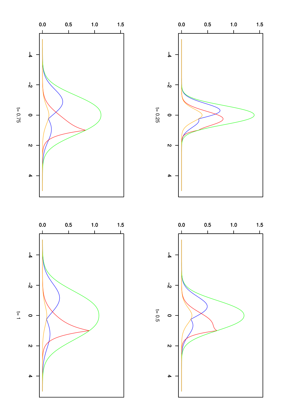
as in Theorem 2.1. In particular, $X$ can be the solution to the following SDE, $dX(t)=b(t,X)dt+dW(t)$ , $X(0)=0$ , $t\geq 0$ , with $b$ bounded and predictable as in Corollary 2.3. Furthermore, denote by $\rho_{t}$ the density of $X(t)$ at a fixed time $t>0$ . Then Theorem 2.1 grants that $0<\alpha_{t}(x)\leq\rho_{t}(x)\leq\beta_{t}(x)$ for any $x\in\mathbb{R}$ . In the following figure we can observe the functions $\alpha_{t}$ and $\beta_{t}$ for different values of $t>0$ and see how they behave. We can see the function $\alpha_{t}$ in orange and $\beta_{t}$ in green. Any density lies between these two curves and these bounds are optimal in the sense that, for given $x_{0},y_{0}\in\mathbb{R}$ we can find drifts $u_{x_{0}}$ and $u_{y_{0}}$ such that the associated densities $\rho_{t}^{x_{0}}$ , resp. $\rho_{t}^{y_{0}}$ for these drift coefficients satisfy $\rho_{t}(x_{0})=\alpha_{t}(x_{0})$ , respectively, $\rho_{t}(y_{0})=\beta_{t}(y_{0})$ . As an illustration we just take the drift to be $+\mathrm{sgn}(x-0.25)$ in blue and $-\mathrm{sgn}(x-1)$ in red.

Refer to caption — Figure 1. Upper and lower bounds for $C=1$ starting at $x=0$ (in green and orange) with the respective densities when the drift coefficients are $\mathrm{sgn}(x-0.25)$ and $-\mathrm{sgn}(x-1)$ (blue and red) at different times $t\in\{0.25,0.5,0.75,1\}$ .

As we can see, both densities are bounded by $\alpha_{t}$ and $\beta_{t}$ and the bounds are attained in $0.25$ for density of the process with drift $+\mathrm{sgn}(x-0.25)$ (in blue) and in $1$ when the drift is $-\mathrm{sgn}(x-1)$ (in red).

3. Reduction and the critical case

In this section we will see how to derive the functions $\alpha_{t,C}$ and $\beta_{t,C}$ explicitly for the case $d=1$ as well as some of their properties, cf. Theorem 3.5. Then we will show that these are indeed the bounds for the densities of any solution to SDEs with bounded measurable drift by solving a stochastic control problem, cf. Theorem 3.13 and thereafter we give the proof for Theorem 2.1. In the sequel, consider the process

\displaystyle Y_{x}^{\pm}(t):=x\pm\int_{0}^{t}\mathrm{sgn}(Y_{x}^{\pm}(s))ds+W(t),\quad t\geq 0,

(1)

c.f. [23] for existence and (pathwise) uniqueness. Moreover, at some point we will also use the property that the solution to equation (1) is strong Markov, even for the multidimensional case. This can be for instance justified using [1, Theorem 6.4.5] in connection with [22, Corollary IX.1.14].

Lemma 3.1.

For every $t>0$ , $Y_{0}^{+}(t)$ resp. $Y_{0}^{-}(t)$ has density $\rho_{Y_{0}^{+}(t)}$ , resp. $\rho_{Y_{0}^{-}(t)}$ given by

	$\displaystyle p_{t}(0,y)$	$\displaystyle:=\rho_{Y_{0}^{+}(t)}=\frac{1}{\sqrt{t}}\varphi\left(\frac{\|y\|-t}{\sqrt{t}}\right)-e^{2\|y\|}\Phi\left(-\frac{\|y\|+t}{\sqrt{t}}\right),\quad\text{resp.}$
	$\displaystyle q_{t}(0,y)$	$\displaystyle:=\rho_{Y_{0}^{-}(t)}=\frac{1}{\sqrt{t}}\varphi\left(\frac{t+\|y\|}{\sqrt{t}}\right)+e^{-2\|y\|}\Phi\left(\frac{t-\|y\|}{\sqrt{t}}\right)$

for $y\in\mathbb{R}$ and any $t>0$ where $\varphi$ , resp. $\Phi$ , denote the density, resp. the distribution function, of the standard normal law.

Proof.

The density for $Y_{0}^{-}(t)$ is the statement of [15, Exercise 6.3.5] as for $Y_{0}^{+}(t)$ computations are fairly similar. ∎

The computation of the densities $\rho_{Y_{0}^{+}(t)}$ and $\rho_{Y_{0}^{-}(t)}$ in the previous lemma are relatively easy given the fact that the local-time of the Brownian motion starting from 0 is symmetric and the joint law of $W(t)$ and the local time of $W$ , $L_{t}^{W}(0)$ is explicitly known, see [15]. Nevertheless, one is able to find reasonably explicit expressions for the densities of $Y_{x}^{+}(t)$ and $Y_{x}^{-}(t)$ which yield representations for $\alpha$ and $\beta$ if $d=1$ .

First we focus on the computation of the density of $Y_{x}^{-}(t)$ and then for $Y_{x}^{+}(t)$ which is similar.

Lemma 3.2.

For every $t\geq 0$ , the density of $Y_{x}^{-}(t)$ is given by

q_{t}(x,y)=\frac{1}{\sqrt{2\pi t}}e^{-\frac{(\mathrm{sgn}(x)(x-y)-t)^{2}}{2t}}\left(1-e^{-\frac{2xy}{t}}\right)1_{\{\mathrm{sgn}(xy)\geq 0\}}+\int_{0}^{t}q_{t-s}(0,y)\rho_{\tau_{0}^{x}}(s)ds

where $x,y\in\mathbb{R}$ , $x\neq 0$ and $\tau_{0}^{x}$ is the first hitting time of the process $Y_{x}^{-}(t)$ at 0 whose density function is explicitly given by

\rho_{\tau_{0}^{x}}(s)=\frac{|x|}{\sqrt{2\pi s^{3}}}e^{-\frac{(|x|-s)^{2}}{2s}},\ s>0.

Proof.

Let $\tau_{0}^{x}$ be the first time the process $Y_{x}^{-}$ hits 0, i.e.

\tau_{0}^{x}:=\inf\{t\geq 0:\ Y_{x}^{-}(t)=0\}.

Then it is clear, that $Y_{x}^{-}(t)=x-\mathrm{sgn}(x)t+W(t)$ for any $t\in[0,\tau_{0}^{x}]$ . Define $\widetilde{W}:=-W$ and $B(t):=\mathrm{sgn}(x)t+\widetilde{W}(t)$ . The process $B(t)$ is a Brownian motion with drift starting at 0. It is clear, that $\tau_{0}^{x}=\inf\{t\geq 0:B(t)=x\}$ , whose law is known, namely $\tau_{0}^{x}$ is inverse Gaussian distributed and [6, p.223, Formula 2.0.2] states that its density is given by

\rho_{\tau_{0}^{x}}(t)=\frac{|x|}{\sqrt{2\pi t^{3}}}e^{-\frac{(|x|-t)^{2}}{2t}},\ t>0.

Now define $f_{\varepsilon}(z):=\frac{1}{2\varepsilon}1_{(y-\varepsilon,y+\varepsilon)}(z)$ for a fixed $y\in\mathbb{R}$ , then

	$\displaystyle\mathrm{E}[f_{\varepsilon}(Y_{x}(t))]$	$\displaystyle=\mathrm{E}[f_{\varepsilon}(Y_{x}^{-}(t))1_{\{t<\tau_{0}^{x}\}}]+\mathrm{E}[f_{\varepsilon}(Y_{x}^{-}(t))1_{\{t\geq\tau_{0}^{x}\}}]$
		$\displaystyle=A_{1}+A_{2}$

where $A_{1}:=\mathrm{E}[f_{\varepsilon}(Y_{x}^{-}(t))1_{\{t<\tau_{0}^{x}\}}]$ and $A_{2}:=\mathrm{E}[f_{\varepsilon}(Y_{x}^{-}(t))1_{\{t\geq\tau_{0}^{x}\}}]$ . We have

	$\displaystyle P\left(Y_{x}^{-}(t)\leq y,t<\tau_{0}^{x}\right)$	$\displaystyle=P\left(x-\mathrm{sgn}(x)t+W(t)\leq y,t<\tau_{0}^{x}\right)$
		$\displaystyle=P\left(B(t)\geq x-y,t<\tau_{0}^{x}\right).$

We start with the case $x>0$ . Observe that $\tau_{0}^{x}=\inf\{t>0:B(t)=x\}$ and hence $\{t<\tau_{0}^{x}\}=\{M(t)<x\}$ where $M(t):=\sup_{s\in[0,t]}B(s)$ . As a consequence

	$\displaystyle P\left(Y_{x}^{-}(t)\leq y,t<\tau_{0}^{x}\right)$	$\displaystyle=P\left(B(t)\geq x-y,M(t)<x\right)$
		$\displaystyle=\mathrm{E}\left[1_{\{B(t)\geq x-y,M(t)<x\}}\right]$
		$\displaystyle=\mathrm{E}_{Q}\left[1_{\{B(t)\geq x-y,M(t)<x\}}\frac{1}{Z(t)}\right]$

where $Q$ is the equivalent measure w.r.t. $P$ defined by

\frac{dQ}{dP}\bigg|_{\mathcal{F}_{t}}=\exp\left\{-\mathrm{sgn}(x)\widetilde{W}(t)-t/2\right\}=:Z(t),\quad t\geq 0.

[20, Theorem 8.6.4] yields that the process $B(t)=\mathrm{sgn}(x)t+\widetilde{W}(t)$ , $t\geq 0$ is a standard $Q$ -Brownian motion and $M(t)$ is therefore the running maximum of the standard Brownian motion $B$ , hence

\displaystyle P\left(Y_{x}^{-}(t)\leq y,t\leq\tau_{0}^{x}\right)=\int_{0}^{\infty}\int_{-\infty}^{w}1_{\{z\geq x-y,w<x\}}e^{\mathrm{sgn}(x)z-t/2}\rho_{B(t),M(t)}(z,w)dzdw

(2)

where $\rho_{B(t),M(t)}$ denotes the joint density of $B(t)$ and $M(t)$ which is explicitly given, see [15, Proposition 2.8.1], by

\rho_{B(t),M(t)}(z,w)=\frac{2(2w-z)}{\sqrt{2\pi t^{3}}}\exp\left\{-\frac{(2w-z)^{2}}{2t}\right\},\ z\leq w,\ w\geq 0.

We have

	$\displaystyle A_{1}$	$\displaystyle=\frac{1}{2\varepsilon}P\left(y-\varepsilon\leq Y_{x}^{-}(t)\leq y+\varepsilon,t\leq\tau_{0}^{x}\right)$
		$\displaystyle=\frac{1}{2\varepsilon}\int_{0}^{\infty}\int_{-\infty}^{w}1_{\{x-y-\varepsilon\leq z\leq x-y+\varepsilon,w<x\}}e^{\mathrm{sgn}(x)z-t/2}\rho_{B(t),M(t)}(z,w)dzdw$

Finally, the above probability converges to the derivative of (2) w.r.t. $y$ , that is

	$\displaystyle\lim_{\varepsilon\searrow 0}$	$\displaystyle\frac{1}{2\varepsilon}P\left(y-\varepsilon\leq Y_{x}^{-}(t)\leq y+\varepsilon,t<\tau_{0}^{x}\right)$
		$\displaystyle=e^{\mathrm{sgn}(x)(x-y)-t/2}\int_{x-y}^{x}\rho_{B(t),M(t)}(x-y,w)dw$
		$\displaystyle=\frac{1}{\sqrt{2\pi t}}e^{\mathrm{sgn}(x)(x-y)-t/2}\left(e^{-(x-y)^{2}/2t}-e^{-(x+y)^{2}/2t}\right)1_{\{x\geq x-y\}}$
		$\displaystyle=\frac{1}{\sqrt{2\pi t}}e^{-\frac{(\mathrm{sgn}(x)(x-y)-t)^{2}}{2t}}\left(1-e^{-\frac{2xy}{t}}\right)1_{\{y\geq 0\}}.$

Now we continue to compute $A_{2}$ . Define the random variable $\tau:=\tau_{0}^{x}\vee t$ . It is readily checked that $\tau\geq\tau_{0}^{x}$ and $\tau$ is $\mathcal{F}_{\tau_{0}^{x}}$ -measurable because the event $\{t\geq\tau_{0}^{x}\}$ is in $\mathcal{F}_{\tau_{0}^{x}}$ . Then the strong Markov property of $Y_{x}^{-}$ and [15, Corollary 2.6.18] yield

	$\displaystyle\mathrm{E}[f_{\varepsilon}(Y_{x}^{-}(t))1_{\{t\geq\tau_{0}^{x}\}}\|\mathcal{F}_{\tau_{0}^{x}}]$	$\displaystyle=\mathrm{E}[f_{\varepsilon}(Y_{x}^{-}(\tau))1_{\{t\geq\tau_{0}^{x}\}}\|\mathcal{F}_{\tau_{0}^{x}}]$
		$\displaystyle=1_{\{t\geq\tau_{0}^{x}\}}\mathrm{E}[f_{\varepsilon}(Y_{x}^{-}(\tau))\|\mathcal{F}_{\tau_{0}^{x}}]$
		$\displaystyle=1_{\{t\geq\tau_{0}^{x}\}}\mathrm{E}[f_{\varepsilon}(Y_{0}^{-}(\xi))]\|_{\xi=\tau-\tau_{0}^{x}}$

$P$ -a.s. As a consequence

	$\displaystyle\mathrm{E}[f_{\varepsilon}(Y_{x}^{-}(t))1_{\{t\geq\tau_{0}^{x}\}}]$	$\displaystyle=\mathrm{E}\left[\mathrm{E}[f_{\varepsilon}(Y_{x}^{-}(t))1_{\{t\geq\tau_{0}^{x}\}}\|\mathcal{F}_{\tau_{0}^{x}}]\right]$
		$\displaystyle=\mathrm{E}\left[1_{\{t\geq\tau_{0}^{x}\}}\mathrm{E}[f_{\varepsilon}(Y_{0}^{-}(\xi))]\|_{\xi=\tau-\tau_{0}^{x}}\right]$
		$\displaystyle=\mathrm{E}\left[1_{\{t\geq\tau_{0}^{x}\}}\mathrm{E}[f_{\varepsilon}(Y_{0}^{-}(\xi))]\|_{\xi=t-\tau_{0}^{x}}\right].$

Now, the density of $Y_{0}^{-}(t)$ is explicitly known by Lemma 3.1. Thus

A_{2}=\mathrm{E}\left[\int_{\mathbb{R}}f_{\varepsilon}(z)q_{t-\tau_{0}^{x}}(0,z)1_{\{t\geq\tau_{0}^{x}\}}\right]=\int_{0}^{t}\int_{\mathbb{R}}f_{\varepsilon}(z)q_{t-s}(0,z)\rho_{\tau_{0}^{x}}(s)ds.

Then, letting $\varepsilon\to 0$ and by Lebesgue’s dominated convergence theorem we obtain that, for $x>0$ and $y\in\mathbb{R}$

q_{t}(x,y)=\frac{1}{\sqrt{2\pi t}}e^{-\frac{(\mathrm{sgn}(x)(x-y)-t)^{2}}{2t}}\left(1-e^{-\frac{2xy}{t}}\right)1_{\{y\geq 0\}}+\int_{0}^{t}q_{t-s}(0,y)\rho_{\tau_{0}^{x}}(s)ds.

We have

	$\displaystyle-Y_{-x}^{-}(t)$	$\displaystyle=x+\int_{0}^{t}\mathrm{sgn}(Y_{-x}^{-}(s))ds+\widetilde{W}(t)$
		$\displaystyle=x-\int_{0}^{t}\mathrm{sgn}(-Y_{-x}^{-}(s))ds+\widetilde{W}(t)$

for any $t\geq 0$ and hence $(-Y_{-x}^{-},\widetilde{W})$ is a weak solution of (1) for $\pm=-$ and starting point $x$ . Hence, $-Y_{-x}^{-}(t)$ has the same law as $Y_{x}^{-}(t)$ for any $t\geq 0$ . Consequently, we have

q_{t}(x,y)=q_{t}(-y,-x),\quad x>0,y\in\mathbb{R}.

The claimed formula follows. ∎

Similarly, we can also obtain the density for $Y_{x}^{+}(t)$ . The proof follows exactly the same ideas as in Lemma 3.2 and has therefore been omitted.

Lemma 3.3.

For every $t\geq 0$ , the density of $Y_{x}^{+}(t)$ is given by

p_{t}(x,y):=\frac{2}{\sqrt{2\pi t}}e^{-\frac{(\mathrm{sgn}(x)(x-y)+t)^{2}}{2t}}\left(1-e^{\frac{-2xy}{t}}\right)1_{\{\mathrm{sgn}(xy)\geq 0\}}+\int_{0}^{t}p_{t-s}(0,y)\rho_{\theta_{0}^{x}}(s)ds.

for $x,y\in\mathbb{R}$ , $x\neq 0$ and $\theta_{0}^{x}$ is the first hitting time of where

\rho_{\theta_{0}^{x}}(s)=\frac{|x|}{\sqrt{2\pi s^{3}}}e^{-\frac{(|x|+s)^{2}}{2s}},\ \ 0<s<\infty.

Proof.

The proof of this lemma follows completely the same ideas as in Lemma 3.2. One of the main differences is that in this case the distribution of the stopping time $\theta_{0}^{x}$ has an atom at infinity, namely, from [6, p.223, Formula 2.0.2] we have

\rho_{\theta_{0}^{x}}(t)=\frac{|x|}{\sqrt{2\pi t^{3}}}e^{-\frac{(|x|+t)^{2}}{2t}},\ 0<t<\infty

and

P(\theta_{0}^{x}=\infty)=1-e^{-2|x|}.

∎

Now we are in a position to define the functions $\alpha_{t,C}$ and $\beta_{t,C}$ for the one-dimensional case and study some of their properties. Before we do that, we will need a technical result to prove one of the properties of these functions.

Proposition 3.4.

Let $b:\mathbb{R}_{+}\times\mathbb{R}\rightarrow\mathbb{R}$ be bounded and measurable and

X_{x}(t):=x+\int_{0}^{t}b(s,X_{x}(s))ds+W(t),\quad x\in\mathbb{R},\quad t\geq 0

where $W$ is a $1$ -dimensional Brownian motion. Then

X_{x}(t)\leq X_{y}(t)\quad P\text{-a.s.}

for any $t\geq 0$ , $x,y\in\mathbb{R}$ with $x\leq y$ .

Proof.

Define

Y_{x}(t):=X_{x}(t)-W(t)=x+\int_{0}^{t}b(s,Y_{x}(s)+W(s))ds=x+\int_{0}^{t}\widetilde{b}(s,Y_{x}(s))ds

where the equalities hold $P$ -a.s. and here $\widetilde{b}(t,z):=b(t,z+W(t))$ for any $t\geq 0$ , $z\in\mathbb{R}$ . Let $x,y\in\mathbb{R}$ with $x\leq y$ and define $Z(t):=\min\{Y_{x}(t),Y_{y}(t)\}$ . Then

Z(t)=x+\int_{0}^{t}\widetilde{b}(s,Z(s))ds,\quad t\geq 0.

Hence $U(t):=Z(t)+W(t)=x+\int_{0}^{t}b(s,U(s))ds+W(t)$ . [22, Theorem IX.3.5 i)] yields $U(t)=X_{x}(t)$ a.s. Observe that $U(t)=\min\{X_{x}(t),X_{y}(t)\}$ and hence

X_{x}(t)=U(t)\leq X_{y}(t),\quad t\geq 0

$P$ -a.s. ∎

Theorem 3.5.

Let $q$ be the transition density of the Markov process $Y^{-}$ which is given in Lemma 3.2 and $p$ the transition density for the Markov process $Y^{+}$ given in Lemma 3.3. Define the functions $\alpha,\beta:\mathbb{R}_{++}\times\mathbb{R}_{+}\times\mathbb{R}\rightarrow(0,\infty)$ by $\alpha_{t,C}(x):=Cp_{tC^{2}}(Cx,0)$ and $\beta_{t,C}(x):=Cq_{tC^{2}}(Cx,0)$ where $t>0$ , $C>0$ and $x\in\mathbb{R}$ . Then

\displaystyle\begin{split}\alpha_{t,C}(x)&=\int_{0}^{tC^{2}}Cp_{tC^{2}-s}(0,0)\rho_{\theta_{0}^{Cx}}(s)ds,\\ &=\int_{0}^{tC^{2}}\left(\frac{C}{\sqrt{tC^{2}-s}}\varphi(\sqrt{tC^{2}-s})-C\Phi(-\sqrt{tC^{2}-s})\right)\rho_{\theta_{0}^{Cx}}(s)ds,\ x\neq 0,\end{split}

(3)

and

\displaystyle\begin{split}\beta_{t,C}(x)&=\int_{0}^{tC^{2}}Cq_{tC^{2}-s}(0,0)\rho_{\tau_{0}^{Cx}}(s)ds\\ &=\int_{0}^{tC^{2}}\left(\frac{C}{\sqrt{tC^{2}-s}}\varphi(\sqrt{tC^{2}-s})+C\Phi(\sqrt{tC^{2}-s})\right)\rho_{\tau_{0}^{Cx}}(s)ds,\quad x\neq 0\end{split}

(4)

where recall that $\rho_{\theta_{0}^{x}}$ , respectively $\rho_{\tau_{0}^{x}}$ are given as in Lemma 3.3, respectively as in Lemma 3.2.

In addition, for each $t>0$ and $C>0$ the functions $\alpha_{t,C}$ and $\beta_{t,C}$ are analytic in $\mathbb{R}\setminus\{0\}$ , Lipschitz continuous in $\mathbb{R}$ , symmetric, decreasing on $[0,\infty)$ and by symmetry increasing on $(-\infty,0]$ . They have exponential decay of the type $o(c_{1}|x|e^{c_{2}|x|}e^{-c_{3}|x|^{2}})$ for constants $c_{1},c_{2},c_{3}>0$ . Moreover, they attain their maxima at $x=0$ which are given by

\alpha_{t,C}(0)=Cp_{tC^{2}}(0,0)=\frac{1}{\sqrt{t}}\varphi\left(C\sqrt{t}\right)-C\Phi\left(-C\sqrt{t}\right)

and

\beta_{t,C}(0)=Cq_{tC^{2}}(0,0)=\frac{1}{\sqrt{t}}\varphi\left(C\sqrt{t}\right)+C\Phi\left(C\sqrt{t}\right).

Proof.

We will carry out a more detailed proof of the properties on $\beta_{t,C}$ . For the case of $\alpha_{t,C}$ the same proof, mutatis mutandis, follows as well.

First of all, observe that $\beta_{t,C}(x)=C\beta_{tC^{2},1}(Cx)$ and hence it is sufficient to carry out the proof for $C=1$ then all properties follow for arbitrary $C>0$ .

At the end of the proof of Lemma 3.2 we have shown that the law of $Y_{x}^{-}(t)$ coincides with the law of $-Y_{-x}^{-}(t)$ . Hence, the symmetry of $\beta_{t,1}$ follows.

To show analyticity, define $f(s,x):=q_{t-s}(0,0)\rho_{\tau_{0}^{x}}(s)$ for $s\in(0,t)$ and $x\in\mathbb{R}\setminus\{0\}$ and the family of domains

\mathbb{S}_{\varepsilon}:=\left\{z\in\mathbb{C}:\ \varepsilon<\mathrm{Re}(z)<\frac{1}{\varepsilon},\ \mathrm{Re}(z)>2|\mathrm{Im}(z)|\right\},

$0<\varepsilon<1$ and $\mathbb{S}:=\cup_{0<\varepsilon<1}\mathbb{S}_{\varepsilon}$ . Then for every $z\in\mathbb{S}$ , $g:\mathbb{R}_{+}\times\mathbb{S}\rightarrow\mathbb{C}$ defined as $g(s,z):=q_{t-s}(0,0)\frac{z}{\sqrt{2\pi s^{3}}}e^{-\frac{(z-s)^{2}}{2s}}$ is the holomorphic extension of $f$ to $\mathbb{S}$ . Let $\epsilon>0$ , $t>0$ and let us check that $z\mapsto\int_{0}^{t}g(s,z)ds$ is holomorphic on $\mathbb{S}_{\varepsilon}$ . We have $|z|\leq\sqrt{5/4}/\epsilon$ , $\mathrm{Re}(z^{2})>3\epsilon^{2}/4$ and hence

	$\displaystyle\|g(s,z)\|$	$\displaystyle\leq\left(\frac{1}{\sqrt{t-s}}+1\right)\frac{1/\varepsilon}{\sqrt{s^{3}}}\|e^{-\frac{z^{2}}{2s}}e^{z}e^{-s/2}\|$
		$\displaystyle\leq\left(\frac{1}{\sqrt{t-s}}+1\right)\frac{1/\varepsilon}{\sqrt{s^{3}}}e^{1/\varepsilon}e^{-\frac{3\varepsilon^{2}}{8s}}$

for any $s\in(0,t)$ , which is integrable on $(0,t)$ for every $\varepsilon>0$ . For a real differentiable function from an open domain in $\mathbb{C}$ to $\mathbb{C}$ we denote the complex conjugate differential operator by $\partial_{\bar{z}}$ . Recall, that such a function is holomorphic if and only if its complex conjugate derivative is zero. So, by changing differentiation and integration, we have

\partial_{\bar{z}}\int_{0}^{t}g(s,z)ds=\int_{0}^{t}\partial_{\bar{z}}g(s,z)ds=0

for every $z\in\mathbb{S}_{\varepsilon}$ where the last follows since $g(t,\cdot)$ is holomorphic on $\mathbb{S}$ for every $t>0$ being thus $\int_{0}^{t}f(s,x)ds$ is analytic on $(0,\infty)$ . For $x<0$ use the symmetry of $\beta_{t,1}$ to conclude.

In addition, $\beta_{t,1}$ is Lipschitz in 0, i.e. there is a constant $K>0$ such that $|\beta_{t,1}(0)-\beta_{t,1}(x)|\leq|x|K$ for any $x\in\mathbb{R}$ . Indeed, write

\displaystyle\int_{0}^{t}q_{t-s}(0,0)\rho_{\tau_{0}^{x}}(s)ds

\displaystyle=E[H(\tau_{0}^{x})]+\int_{t/2}^{t}q_{t-s}(0,0)\rho_{\tau_{0}^{x}}(s)(1-h(s))ds

where $H(s):=q_{t-s}(0,0)h(s)$ where $h$ is some function which is bounded by $1$ , constant $1$ near zero, constant $0$ on $[t/2,t]$ and $h\in C^{\infty}([0,t],\mathbb{R})$ .

We see that $H$ is Lipschitz continuous with some Lipschitz constant $L>0$ and, hence,

|\mathrm{E}[H(\tau_{0}^{x})]-\mathrm{E}[H(\tau_{0}^{0})]|\leq L(\mathrm{E}\tau_{0}^{x}-\mathrm{E}\tau_{0}^{0})=L|x|

for any $x>0$ . Moreover,

\displaystyle\int_{t/2}^{t}q_{t-s}(0,0)\rho_{\tau_{0}^{x}}(s)(1-h(s))ds\leq|x|\frac{1}{\sqrt{t}}\frac{2}{\pi}\int_{1/2}^{1}\left(\frac{1}{\sqrt{2\pi t}}\frac{1}{\sqrt{1-s}}+1\right)ds

(5)

which implies that

|\beta_{t,1}(0)-\beta_{t,1}(x)|\leq|x|K

for some constant $K>0$ . Together with the analyticity outside zero we conclude that $\beta_{t,1}$ is locally Lipschitz continuous. If we have shown that $\beta_{t,1}$ is decreasing on $[0,\infty)$ , then it follows that $\beta_{t,1}$ is globally Lipschitz continuous because it is positive valued.

For monotonicity, it is sufficient to show that $\beta_{t,1}$ is decreasing on $(0,\infty)$ and then symmetry and continuity yield the claimed growth properties. Consider $x\in(0,\infty)$ and $v_{t}^{\varepsilon}(x):=\mathrm{E}\left[f_{\varepsilon}(Y_{x}^{-}(t))\right]$ where $f_{\varepsilon}(y)=1_{\{|y|<\varepsilon\}}$ . Here, $\beta_{t,1}(x)$ is defined as the density of $Y_{x}^{-}(t)$ at 0. Hence, $\beta_{t,1}(x)=p_{t}(x,0)=\lim_{\varepsilon\searrow 0}\frac{1}{\varepsilon}v_{t}^{\varepsilon}(x)$ . Thus it is enough to show that $v_{t}^{\varepsilon}(x)$ is decreasing on $(0,\infty)$ for every ${\varepsilon}>0$ . Let $0<x<y<\infty$ . Proposition 3.4 yields $P(\forall t\geq 0:Y_{y}^{-}(t)\geq Y_{x}^{-}(t))=1.$ Define $\tau:=\inf\{t>0:\ -Y_{x}^{-}(t)=Y_{y}^{-}(t)\}$ . [10, Proposition 2.1.5 a)] yields that $\tau$ is a stopping time because it is the first contact time with the closed set $\{0\}$ of the continuous process $Y_{x}^{-}+Y_{y}^{-}$ . Observe, that $|Y_{x}^{-}(t)|\leq Y_{y}^{-}(t)$ for any $t\in[0,\tau]$ . We can write

	$\displaystyle v_{t}^{\varepsilon}(y)-v_{t}^{\varepsilon}(x)$	$\displaystyle=\mathrm{E}\left[\left(1_{\{\|Y_{y}^{-}(t)\|<\varepsilon\}}-1_{\{\|Y_{x}^{-}(t)\|<\varepsilon\}}\right)1_{\{t<\tau\}}\right]$
		$\displaystyle+\mathrm{E}\left[\left(1_{\{\|Y_{y}^{-}(t)\|<\varepsilon\}}-1_{\{\|Y_{x}^{-}(t)\|<\varepsilon\}}\right)1_{\{t\geq\tau\}}\right]$
		$\displaystyle=C_{1}+C_{2}$

where $C_{1}:=\mathrm{E}\left[\left(1_{\{|Y_{y}^{-}(t)|<\varepsilon\}}-1_{\{|Y_{x}^{-}(t)|<\varepsilon\}}\right)1_{\{t<\tau\}}\right]$ and $C_{2}$ is the other summand. It can be seen that $C_{1}$ is negative since $P(|Y_{x}^{-}(t)|\leq\varepsilon,t<\tau)\geq P(|Y_{y}^{-}(t)|\leq\varepsilon,t<\tau)$ . For the term $C_{2}$ we use exactly the same Markov-argument as for the term $A_{2}$ in Lemma 3.2 by defining $\tilde{\tau}:=\tau\vee t$ . Then $\tilde{\tau}\geq\tau$ and $\tilde{\tau}$ is $\mathcal{F}_{\tau}$ -measurable. Thus, the strong Markov property of $Y_{x}^{-}$ and $Y_{y}^{-}$ and [15, Corollary 2.6.18] yield

	$\displaystyle\mathrm{E}\left[1_{\{\|Y_{y}^{-}(t)\|<\varepsilon\}}1_{\{t\geq\tau\}}\|\mathcal{F}_{\tau}\right]$	$\displaystyle=\mathrm{E}\left[1_{\{\|Y_{y}^{-}(\tilde{\tau})\|<\varepsilon\}}1_{\{t\geq\tau\}}\|\mathcal{F}_{\tau}\right]$
		$\displaystyle=1_{\{t\geq\tau\}}\mathrm{E}\left[1_{\{\|Y_{y}^{-}(\tilde{\tau})\|<\varepsilon\}}\|\mathcal{F}_{\tau}\right]$
		$\displaystyle=1_{\{t\geq\tau\}}\mathrm{E}\left[1_{\{\|Y_{y}^{-}(\xi)\|<\varepsilon\}}\|_{\xi=\tilde{\tau}-\tau}\right]$

P-a.s. On the other hand, observe that $Y_{y}^{-}(\tau)=-Y_{x}^{-}(\tau)$ by the definition of $\tau$ . So

1_{\{t\geq\tau\}}\mathrm{E}\left[1_{\{|Y_{y}^{-}(\xi)|<\varepsilon\}}|_{\xi=\tilde{\tau}-\tau}\right]=1_{\{t\geq\tau\}}\mathrm{E}\left[1_{\{|-Y_{x}^{-}(\xi)|<\varepsilon\}}|_{\xi=\tilde{\tau}-\tau}\right]

which implies that $C_{2}=0$ . As a result

v_{t}^{\varepsilon}(y)-v_{t}^{\varepsilon}(x)=\mathrm{E}\left[\left(1_{\{|Y_{y}^{-}(t)|<\varepsilon\}}-1_{\{|Y_{x}^{-}(t)|<\varepsilon\}}\right)1_{\{t<\tau\}}\right]\leq 0

which implies

\beta_{t}(y)-\beta_{t}(x)=\lim_{\varepsilon\searrow 0}\frac{1}{\varepsilon}(v_{t}^{\varepsilon}(y)-v_{t}^{\varepsilon}(x))\leq 0

for every $x,y\in\mathbb{R}$ with $0<x<y$ .

Finally, we show that $\beta_{t,1}$ has exponential tails. Observe that $|q_{t-s}(0,0)|\leq\frac{1}{\sqrt{2\pi(t-t/2)}}+1$ for $s\in[0,t/2]$ and thus

\displaystyle\int_{0}^{t/2}|q_{t-s}(0,0)|\frac{|x|}{\sqrt{2\pi s^{3}}}e^{-\frac{(|x|-s)^{2}}{2s}}\leq K|x|e^{|x|}\int_{0}^{t/2}s^{-3/2}e^{-\frac{|x|^{2}}{2s}}ds

where $K$ denotes the collection of constants not depending on $x>0$ . Moreover, one can show that

\int_{0}^{t/2}s^{-3/2}e^{-\frac{|x|^{2}}{2s}}ds\leq K\frac{1}{|x|^{2}}e^{-\frac{|x|^{2}}{2t}}

for a constant $K>0$ independent of $x$ . Altogether

\int_{0}^{t/2}|q_{t-s}(0,0)|\frac{|x|}{\sqrt{2\pi s^{3}}}e^{-\frac{(|x|-s)^{2}}{2s}}\leq K\frac{e^{|x|}}{|x|}e^{-\frac{|x|^{2}}{2t}}.

Finally, $|\rho_{\tau_{0}^{x}}(s)|\leq K|x|e^{-\frac{(|x|-t)^{2}}{2t}}$ for $s\in[t/2,t]$ , $|x|>t$ which yields

\int_{t/2}^{t}|q_{t-s}(0,0)||\rho_{\tau_{0}^{x}}(s)|ds\leq K|x|e^{-\frac{(|x|-t)^{2}}{2t}}.

∎

From now on, let us consider the processes $Y_{x}^{-}$ and $Y_{x}^{+}$ given in Equation (1) for the multidimensional case, i.e. $x\in\mathbb{R}^{d}$ , $\mathrm{sgn}(x):=\frac{x}{|x|}1_{\{x\neq 0\}}$ and $W$ a $d$ -dimensional standard Brownian motion. We denote $x=(x_{1},\dots,x_{d})\in\mathbb{R}^{d}$ , $W=(W_{1},\dots,W_{d})$ and $Y_{x}^{\pm}(t)=(Y_{x,1}^{\pm}(t),\dots,Y_{x,d}^{\pm}(t))$ . Theorem 2.1 guarantees that the density of any adapted process $X_{u}(t):=\int_{0}^{t}u(s)ds+W(t)$ , $u\in\mathcal{A}$ , has bounds $\alpha_{d,t}:=\alpha_{d,t,1}$ and $\beta_{d,t}:=\beta_{d,t,1}$ .

We start with a proposition which gives a different view on the functions $\alpha_{d,t,C}$ and $\beta_{d,t,C}$ . Namely, we define $Z_{x}^{\pm}(t):=|Y_{x}^{\pm}(t)|^{2}$ with $Z_{x}^{\pm}(0)=|x|^{2}$ and denote $V_{\varepsilon}$ the volume of the $d$ -dimensional Euclidean ball of radius $\varepsilon$ then we have

\alpha_{t,C}(x)=\limsup_{\epsilon\rightarrow 0}\frac{P(|Y_{x}^{+}(t)|\leq\epsilon)}{V_{\epsilon}}=\limsup_{\epsilon\rightarrow 0}\frac{P(Z_{x}^{+}(t)\leq\epsilon^{2})}{C_{d}\ \epsilon^{d}},

and

\beta_{t,C}(x)=\limsup_{\epsilon\rightarrow 0}\frac{P(|Y_{x}^{-}(t)|\leq\epsilon)}{V_{\epsilon}}=\limsup_{\epsilon\rightarrow 0}\frac{P(Z_{x}^{-}(t)\leq\epsilon^{2})}{C_{d}\ \epsilon^{d}},

cf. Theorem 2.1, where $C_{d}:=\frac{\pi^{d/2}}{\Gamma\left(\frac{d}{2}+1\right)}$ . In view of this equality, we are interested in the behaviour of the transition density of $(Z_{x})_{x\in\mathbb{R}}$ near zero which will be exploited in Theorem 3.7 below.

Proposition 3.6.

Let $(\Omega,(\mathcal{F}_{t})_{t\geq 0},\mathfrak{A},P)$ be a filtered probability space. Let $W$ be a $d$ -dimensional Brownian motion and $Y_{x}^{\pm}$ be the solution to the SDE

Y_{x}^{\pm}(t):=x\pm\int_{0}^{t}\mathrm{sgn}(Y_{x}^{\pm}(s))ds+W(t),\quad t\geq 0

for any $x\in\mathbb{R}^{d}$ . Define $Z_{x}^{\pm}(t):=|Y_{x}^{\pm}(t)|^{2}$ , $B_{x}^{\pm}(t):=\int_{0}^{t}\mathrm{sgn}(Y_{x}^{\pm}(s))dW(s)$ for any $x\in\mathbb{R}^{d}$ , $t\geq 0$ . Then $(Z_{x}^{\pm},B_{x}^{\pm})$ is a solution to the SDE

\displaystyle dZ_{x}^{\pm}(t)=\left(d\pm 2\sqrt{Z_{x}^{\pm}(t)}\right)dt+2\sqrt{Z_{x}^{\pm}(t)}dB_{x}^{\pm}(t),\quad Z_{x}^{\pm}(0)=|x|^{2},\quad t\geq 0

(6)

for which pathwise uniqueness holds.

Proof.

Let $f:\mathbb{R}^{d}\rightarrow\mathbb{R}_{+},x\mapsto|x|^{2}$ . Then $Df(x)\cdot y=2\langle x,y\rangle$ and $H_{2}f(x)=2I_{d}$ for any $x,y\in\mathbb{R}^{d}$ where $Df$ denotes the Fréchet differential of $f$ , $H_{2}f$ the Hessian matrix of $f$ and $I_{d}$ denotes the unit matrix in $\mathbb{R}^{d\times d}$ . Itô’s formula yields

	$\displaystyle Z_{x}^{\pm}(t)$	$\displaystyle=\|x\|^{2}+\int_{0}^{t}(\pm 2\langle Y_{x}^{\pm}(s),\mathrm{sgn}(Y_{x}^{\pm}(s))\rangle+d)ds+\int_{0}^{t}2Y_{x}^{\pm}(s)dW(s)$
		$\displaystyle=\|x\|^{2}+\int_{0}^{t}(\pm 2\sqrt{Z_{x}^{\pm}(s)}+d)ds+\int_{0}^{t}2\sqrt{Z_{x}^{\pm}(s)}dB_{x}^{\pm}(s)$

for any $t\geq 0$ . Since $B_{x}^{\pm}$ is a Brownian motion, $(Z_{x}^{\pm},B_{x}^{\pm})$ is a weak solution as required.

It remains to show that the SDE has unique weak solutions. Let $Q$ be a measure, equivalent to $P$ , such that $\widetilde{W}^{\pm}(t):=B_{x}^{\pm}(t)-t$ is a standard $Q$ -Brownian motion. Then the SDE can be rewritten as

\displaystyle dZ_{x}^{\pm}(t)=\left(d\right)dt\pm 2\sqrt{Z_{x}^{\pm}(t)}d\widetilde{W}^{\pm}(t),\quad Z_{x}^{\pm}(0)=|x|^{2},\quad t\geq 0.

(7)

[22, Theorem IX.3.5 ii)] yields that pathwise uniqueness holds for SDE (7) under $Q$ . ∎

The following result gives explicit bounds for the functions $\alpha_{d,t}$ and $\beta_{d,t}$ .

Theorem 3.7.

We have

\frac{2^{d}}{C_{d}d^{d/2}}\prod_{i=1}^{d}\alpha_{1,t}(x_{i})\leq\alpha_{d,t}(x)\leq\beta_{d,t}(x)\leq\frac{2^{d}}{C_{d}}\prod_{i=1}^{d}\beta_{1,t}(x_{i}),\quad x\in\mathbb{R}^{d}

where $C_{d}:=\frac{\pi^{d/2}}{\Gamma\left(\frac{d}{2}+1\right)}$ .

Proof.

Since the proof is fairly similar for $\alpha_{d,t}$ , we will just show the last inequality.

Define the processes $Z_{x,i}^{-}(t):=|Y_{x,i}^{-}(t)|^{2}$ , $i=1,\dots,d$ . Itô’s formula yields

	$\displaystyle Z_{x,i}^{-}(t)$	$\displaystyle=\|x_{i}\|^{2}+\int_{0}^{t}\left(1-2\sqrt{Z_{x,i}^{-}(s)}\frac{\|Y_{x,i}^{-}(s)\|}{\|Y_{x}^{-}(s)\|}\right)ds+2\int_{0}^{t}Y_{x,i}^{-}(s)dW_{i}(s)$
		$\displaystyle=\|x_{i}\|^{2}+\int_{0}^{t}\left(1-2\sqrt{Z_{x,i}^{-}(s)}\frac{\|Y_{x,i}^{-}(s)\|}{\|Y_{x}^{-}(s)\|}\right)ds+2\int_{0}^{t}\sqrt{Z_{x,i}^{-}(s)}dB_{i}(s)$
		$\displaystyle\geq\|x_{i}\|^{2}+\int_{0}^{t}\left(1-2\sqrt{Z_{x,i}^{-}(s)}\right)ds+2\int_{0}^{t}\sqrt{Z_{x,i}^{-}(s)}dB_{i}(s)$

where $B_{i}(t):=\int_{0}^{t}\mathrm{sgn}(Y_{x,i}^{-}(s))dW_{i}(s)$ defines a new standard Brownian motion w.r.t. $P$ . [22, Theorem IV.3.6] and Itô isometry ensure that $(B_{1},\dots,B_{d})$ is a $d$ -dimensional standard Brownian motion. Let $V_{i}$ be the solution of the SDE

\displaystyle V_{i}(t)=|x_{i}|^{2}+\int_{0}^{t}\left(1-2\sqrt{V_{i}(s)}\right)ds+2\int_{0}^{t}\sqrt{V_{i}(s)}dB_{i}(s)

(8)

for any $i=1,\dots,d$ and $Q$ be the measure, equivalent to $P$ , such that $\widetilde{B}(t):=B(t)-(t,\dots,t)$ is a $Q$ -Brownian motion where $B=(B_{1},\dots,B_{d})$ . Then, we have

	$\displaystyle Z_{x,i}^{-}(t)$	$\displaystyle=\|x_{i}\|^{2}+\int_{0}^{t}\left(1+2\sqrt{Z_{x,i}^{-}(s)}\left(1-\frac{\|Y_{x,i}^{-}(s)\|}{\|Y_{x}^{-}(s)\|}\right)\right)ds+2\int_{0}^{t}\sqrt{Z_{x,i}^{-}(s)}d\widetilde{B}_{i}(s),$
	$\displaystyle V_{i}(t)$	$\displaystyle=\|x_{i}\|^{2}+\int_{0}^{t}1ds+2\int_{0}^{t}\sqrt{V_{i}(s)}d\widetilde{B}_{i}(s).$

Similar arguments as in the proof of [22, Theorem IX.3.7] show that $Z_{x,i}^{-}(t)\geq V_{i}(t)$ for any $t\geq 0$ , $Q$ -a.s.

Observe that pathwise uniqueness holds for Equation (6) by Proposition 3.6 and hence [22, Theorem IX.1.7 ii)] states that $V_{i}$ is a strong solution to Equation (8). Consequently, $V_{i}$ is $\sigma(B_{i})$ -measurable and hence $V_{1},\dots,V_{d}$ are independent processes.

Now given $a=(a_{1},\dots,a_{d})\in\mathbb{R}^{d}$ one has $|a|\geq\max{\{|a_{i}|,i=1,\dots,d\}}$ . This implies

	$\displaystyle P(\|Y_{x}^{-}(t)\|\leq\varepsilon)$	$\displaystyle\leq P\left(\bigcap_{i=1}^{d}\{\|Y_{x,i}^{-}(t)\|\leq\varepsilon\}\right)$
		$\displaystyle=P\left(\bigcap_{i=1}^{d}\{Z_{x,i}^{-}(t)\leq\varepsilon^{2}\}\right)$
		$\displaystyle\leq\prod_{i=1}^{d}P\left(V_{i}(t)\leq\varepsilon^{2}\right)$

where in the last step we use the inequalities $Z_{x,i}^{-}(t)\geq V_{i}(t)$ for every $t\geq 0$ , $P$ -a.s. and the fact that $V_{1},\dots,V_{d}$ are independent processes.

By Proposition 3.6 the law of $V_{i}(t)$ under $P$ is the same as the law of $|A_{i}(t)|^{2}$ under $P$ where

A_{i}(t)=x_{i}-\int_{0}^{t}\mathrm{sgn}(A_{i}(s))ds+W_{i}(t),\quad t\geq 0

and the law of $A_{i}(t)$ is given in Lemma 3.2. Hence, we have

	$\displaystyle\beta_{d,t}(x)$	$\displaystyle\xleftarrow{\varepsilon\to 0}\frac{P(\|Y_{x}^{-}(t)\|\leq\varepsilon)}{C_{d}\varepsilon^{d}}$
		$\displaystyle\leq\frac{1}{C_{d}}\prod_{i=1}^{d}\frac{P(\|A_{i}(t)\|\leq\varepsilon)}{\varepsilon}$
		$\displaystyle\xrightarrow{\varepsilon\to 0}\frac{2^{d}}{C_{d}}\prod_{i=1}^{d}\beta_{1,t}(x_{i})$

for any $t>0$ . ∎

In order to prepare our main result of this section we will start with a series of lemmas which aims at showing the continuity condition of [14, Theorem IX.2.11]. The needed continuity condition is summarised in Lemma 3.11.

Lemma 3.8.

Let $(\Omega,(\mathcal{F}_{t})_{t\geq 0},\mathfrak{A},P)$ be a filtered probability space. Let $\varphi:\mathbb{R}_{+}\rightarrow[0,1]$ such that $\varphi$ is infinitely differentiable, $\varphi$ is constant $1$ on $[0,1]$ and constant $0$ on $[2,\infty)$ . Define

A_{k}:\mathbb{R}_{+}\times\mathbb{D}(\mathbb{R}^{d})\rightarrow\mathbb{R},(t,f)\mapsto\int_{0}^{t}\varphi(k|f(s)|)ds

for any $k\in\mathbb{N}$ . Let $b:\Omega\times\mathbb{R}_{+}\rightarrow\mathbb{R}^{d}$ be an adapted process which is bounded by $1$ , $x\in\mathbb{R}^{d}$ and define

X(t):=x+\int_{0}^{t}b(s)ds+W(t),\quad t\geq 0.

Then $\mathrm{E}(A_{k}(t,X))\leq\sqrt{tc_{k}(t)}\exp(t/2)$ where $c_{k}(t):=\mathrm{E}(A_{k}(t,x+W))\rightarrow 0$ for $k\rightarrow\infty$ .

Proof.

Define $Z(t):=\mathcal{E}(-\int_{0}^{t}b(s)dW(s))=1-\int_{0}^{t}Z(s)b(s)dW(s)$ and $dQ|_{\mathcal{F}_{t}}:=Z_{t}dP|_{\mathcal{F}_{t}}$ . Then Girsanov’s theorem [14, Theorem III.3.24] yields that $X$ is a $Q$ -Brownian motion starting in $x$ . Define $Y(t):=1/Z(t)$ . Then

Y(t)=1+\int_{0}^{t}Y(s)b(s)dX(s),\quad t\geq 0

and hence by Gronwall’s lemma, see e.g. [22, Appendix $\lx@sectionsign$ 1], $\mathrm{E}_{Q}(Y(t)^{2})\leq\exp(t)$ . We have

	$\displaystyle\mathrm{E}(A_{k}(t,X))$	$\displaystyle=\mathrm{E}_{Q}\left(A_{k}(t,X)Y(t)\right)$
		$\displaystyle\leq\sqrt{\mathrm{E}_{Q}(A_{k}(t,X)^{2})}\sqrt{\mathrm{E}_{Q}(Y^{2}(t))}$
		$\displaystyle\leq\sqrt{t\mathrm{E}_{Q}(A_{k}(t,X))}\exp(t/2)$
		$\displaystyle=\sqrt{tc_{k}(t)}\exp(t/2)$

for any $t\geq 0$ where we used the Cauchy-Schwartz inequality twice and the fact that $\varphi^{2}\leq\varphi$ . We have

	$\displaystyle c_{k}(t)$	$\displaystyle=\mathrm{E}(A_{k}(t,x+W))$
		$\displaystyle\rightarrow\mathrm{E}(\lambda(\{s\in[0,t]:x+W(s)=0\})$
		$\displaystyle=0$

for $k\rightarrow\infty$ by Lebesgue’s dominated convergence theorem where $\lambda$ denotes the Lebesgue measure on $\mathbb{R}$ . ∎

Lemma 3.9.

Let $(\Omega,(\mathcal{F}_{t})_{t\geq 0},\mathfrak{A},P)$ be a filtered probability space and $W$ be a $d$ -dimensional standard Brownian motion. Let $(A_{k})_{k\in\mathbb{N}}$ and $(c_{k})_{k\in\mathbb{N}}$ be as in Lemma 3.8. Let $(M_{n})_{n\in\mathbb{N}}$ be a sequence of processes that converges in probability to $W$ . For any $n\in\mathbb{N}$ let $b_{n}:\Omega\times\mathbb{R}_{+}\rightarrow\mathbb{R}^{d}$ be an adapted process which is bounded by $1$ , $x\in\mathbb{R}^{d}$ and define

\displaystyle X_{n}(t):=x+\int_{0}^{t}b_{n}(s)ds+M_{n}(t),\quad t\geq 0.

Also, assume that $(X_{n})_{n\in\mathbb{N}}$ converges in distribution to some process $X_{\infty}$ .

Then $X_{\infty}$ has $P$ -a.s. continuous sample paths and

\mathrm{E}A_{k}(t,X_{\infty})\leq\sqrt{tc_{k}(t)}\exp(t/2),\quad t\geq 0,\quad k\in\mathbb{N}.

Moreover, $\lambda\{s\in\mathbb{R}_{+}:X_{\infty}(s)=0\}=0$ $P$ -a.s. where $\lambda$ denotes the Lebesgue measure on $\mathbb{R}$ .

Proof.

Define $Y_{n}(t):=x+\int_{0}^{t}b_{n}(s)ds+W(t)$ , $t\geq 0$ . Then

X_{n}-Y_{n}=M_{n}-W\rightarrow 0

in probability for $n\rightarrow\infty$ . Hence, $Y_{n}\rightarrow X_{\infty}$ in distribution. Since $Y_{n}$ has continuous sample paths for any $n\in\mathbb{N}$ , $X_{\infty}$ has $P$ -a.s. continuous sample paths. Let $t,\epsilon>0$ . Since $A_{k}$ is continuous we have $\mathrm{E}A_{k}(t,X_{\infty})\leq\epsilon+\mathrm{E}A_{k}(t,Y_{n})$ for some $n\in\mathbb{N}$ . Hence, by Lemma 3.8 we have

	$\displaystyle\mathrm{E}A_{k}(t,X_{\infty})$	$\displaystyle\leq\epsilon+\mathrm{E}A_{k}(t,Y_{n})$
		$\displaystyle\leq\epsilon+\sqrt{tc_{k}(t)}\exp(t/2).$

Thus, we have

	$\displaystyle\mathrm{E}(\lambda\{s\in[0,t]:X_{\infty}(s)=0\})$	$\displaystyle\leftarrow\mathrm{E}A_{k}(t,X_{\infty})$
		$\displaystyle\rightarrow 0$

for $k\rightarrow\infty$ and $t\geq 0$ . Thus $\mathrm{E}(\lambda\{s\in\mathbb{R}_{+}:X_{\infty}(s)=0\})\leq\sum_{n=1}^{\infty}\mathrm{E}(\lambda\{s\in[0,n]:X_{\infty}(s)=0\})=0$ . The claim follows. ∎

Remark 3.10.

Let $x\in\mathbb{R}^{d}\backslash\{0\}$ , $\epsilon\in(0,|x|)$ and $y\in\mathbb{R}^{d}$ such that $|x-y|\leq\epsilon$ . Then

|\mathrm{sgn}(x)-\mathrm{sgn}(y)|\leq\sqrt{2}\left(\frac{\epsilon}{|x|}\right).

Lemma 3.11.

Let $(\Omega,(\mathcal{F}_{t})_{t\geq 0},\mathfrak{A},P)$ be a filtered proability space and $W$ be a $d$ -dimensional standard Brownian motion. Let $(b_{n})_{n\in\mathbb{N}}$ be adapted processes which are bounded by $1$ . Let $x\in\mathbb{R}^{d}$ , $(M_{n})_{n\in\mathbb{N}}$ be a sequence of adapted processes which converges in probability to $W$ and define

X_{n}(t):=x+\int_{0}^{t}b_{n}(s)ds+M_{n}(t).

Assume that $(X_{n})_{n\in\mathbb{N}}$ converges in distribution to some process $X_{\infty}$ and define

B:\mathbb{R}_{+}\times\mathbb{D}(\mathbb{R}^{d})\rightarrow\mathbb{R}^{d},(t,f)\mapsto-\int_{0}^{t}\mathrm{sgn}(f(s))ds,\quad t\geq 0

Then $f\mapsto B(t,f)$ is $P^{X_{\infty}}$ -a.s. continuous for any $t\geq 0$ .

Proof.

Let $A_{k}$ be as in Lemma 3.8 for any $k\in\mathbb{N}$ . Lemma 3.9 yields

\lambda\{s\in\mathbb{R}_{+}:X_{\infty}(s)=0\}=0

$P$ -a.s. and hence $A_{k}(X_{\infty},t)\rightarrow 0$ for $k\rightarrow\infty$ $P$ -a.s.

Let $t\geq 0$ and $f,g_{k}\in\mathbb{D}(\mathbb{R}^{d})$ such that $\sup\{|f(s)-g_{k}(s)|:s\leq t\}\leq 1/k^{2}$ for any $k\in\mathbb{N}$ . Then, we have

	$\displaystyle\|B(t,f)-B(t,g_{k})\|\leq$	$\displaystyle\int_{0}^{t}\|\mathrm{sgn}(f(s))-\mathrm{sgn}(g_{k}(s))\|ds$
	$\displaystyle=$	$\displaystyle\int_{0}^{t}\|\mathrm{sgn}(f(s))-\mathrm{sgn}(g_{k}(s))\|1_{\{\|f(s)\|\leq 1/k\}}ds$
		$\displaystyle+\int_{0}^{t}\|\mathrm{sgn}(f(s))-\mathrm{sgn}(g_{k}(s))\|1_{\{\|f(s)\|>1/k\}}ds$
	$\displaystyle\leq$	$\displaystyle 2\int_{0}^{t}1_{\{\|f(s)\|\leq 1/k\}}ds+t\sqrt{2}/k$
	$\displaystyle\leq$	$\displaystyle 2\int_{0}^{t}\varphi(k\|f(s)\|)ds+t\sqrt{2}/k$
	$\displaystyle=$	$\displaystyle 2A_{k}(t,f)+t\sqrt{2}/k$
	$\displaystyle\rightarrow$	$\displaystyle 0$

$P^{X_{\infty}}$ -a.s. for $k\rightarrow\infty$ where we used the integral inequality, then we split the support of $f$ , Remark 3.10 with $\epsilon=1/k^{2}$ and the inequality $1_{[0,1]}(x)\leq\varphi(x)$ for any $x\geq 0$ . ∎

In the next lemma the martingales $M_{n}$ converge to the Brownian motion $W$ but they, and hence the drift in $X_{n}$ , are not adapted to the same Brownian motion. We show that they converge in our specific set-up.

Lemma 3.12.

Let $(\Omega,(\mathcal{F}_{t})_{t\geq 0},\mathfrak{A},P)$ be a filtered probability space. Let $W$ be a $d$ -dimensional Brownian motion, $x\in\mathbb{R}^{d}$ and $M_{n}(t):=W(\theta_{n}(t))$ where $\theta_{n}(t):=\inf\{k/n:t<k/n\}$ for any $n\in\mathbb{N}$ . Assume that $X_{n}(t)=x-\int_{0}^{t}\mathrm{sgn}(X_{n}(s))ds+M_{n}(t)$ for any $n\in\mathbb{N}$ . Then $(X_{n})_{n\in\mathbb{N}}$ converges in distribution to the solution $X$ of the SDE

\displaystyle X(t)=x-\int_{0}^{t}\mathrm{sgn}(X(s))ds+W(t),\quad t\geq 0.

(9)

Proof.

By an independent enlargement of $\mathcal{F}_{0}$ -argument, we may assume that there is a sequence $(H_{n})_{n\in\mathbb{N}}$ of random variables which are indepent of $W$ , $\mathcal{F}_{0}$ -measurable and that $H_{n}$ is centered normal on $\mathbb{R}^{d}$ with variance $I_{d}/n$ where $I_{d}$ denotes the identity matrix in $\mathbb{R}^{d\times d}$ .

Define $\tilde{\theta}_{n}(t):=\theta_{n}(t)-1/n=\max\{k/n:k\geq 0,k/n\leq t\}$ for any $n\in\mathbb{N}$ . Then $0\leq\tilde{\theta}_{n}(t)\leq t$ . Define the $\mathcal{F}$ -adapted process $\widetilde{M}_{n}(t):=H_{n}+W(\widetilde{\theta}_{n}(t))$ and $\widetilde{X}_{n}(t)=x-\int_{0}^{t}\mathrm{sgn}(\widetilde{X}_{n}(s))ds+\widetilde{M}_{n}(t)$ . Then $M_{n}$ has the same law as $\widetilde{M}_{n}$ and, consequently, $(X_{n},M_{n})$ has the same law as $(\widetilde{X}_{n},\widetilde{M}_{n})$ for any $n\in\mathbb{N}$ . Moreover, $\widetilde{M}_{n}\rightarrow W$ in probability.

Define

	$\displaystyle B(t,f)$	$\displaystyle:=-\int_{0}^{t}\mathrm{sgn}(f(s))ds,$
	$\displaystyle C(t,f)$	$\displaystyle:=tI_{d},$
	$\displaystyle\nu(A\times I)$	$\displaystyle:=0,$
	$\displaystyle B_{n}(t)$	$\displaystyle:=B(t,\widetilde{X}_{n}),$
	$\displaystyle C_{n}(t)$	$\displaystyle:=0I_{d}=0,$
	$\displaystyle\nu_{n}(A\times I)$	$\displaystyle:=\mu_{n}(A)\sum_{k=1}^{\infty}\delta_{k/n}(I)$

for any $t\in\mathbb{R}_{+}$ , $f\in\mathbb{D}(\mathbb{R}^{d})$ , $n\in\mathbb{N}$ , $A\in\mathcal{B}(\mathbb{R}^{d})$ , $I\in\mathcal{B}(\mathbb{R}_{+})$ where $\mu_{n}$ is the centered normal law with covariance matrix $I_{d}/n$ . Then $(B_{n},C_{n},\nu_{n})$ is the semimartingale characteristics of $X_{n}$ in the sense of [14, Definition II.2.6] relative to the truncation function $h(x):=\mathrm{sgn}(x)(|x|\wedge 1)$ , $x\in\mathbb{R}^{d}$ . Observe that $(B_{n},C_{n},\nu_{n})_{n\in\mathbb{N}}$ and $(B,C,\nu)$ fulfil the conditions $[\mathrm{Sup-}\beta_{7}]$ , $[\mathrm{Sup-}\gamma_{7}]$ and $[\mathrm{Sup-}\delta_{7,1}]$ in the sense of [14, page 535]. Thus [14, Theorem IX.3.9] states that $(\widetilde{X}_{n})_{n\in\mathbb{N}}$ is tight. Let $(\widetilde{X}_{n_{j}})_{j\in\mathbb{N}}$ be a subsequence of $(\widetilde{X}_{n})_{n\in\mathbb{N}}$ which converges in law and denote the limiting law by $P_{\infty}$ . Lemma 3.11 yields that $B$ is $P_{\infty}$ -a.s. continuous. Let $Y$ be the canonical process on the canonical space $(\mathbb{D}(\mathbb{R}^{d}),(\mathcal{G}_{t})_{t\geq 0},\mathcal{B}(\mathbb{D}(\mathbb{R}^{d})))$ . Then [14, Theorem IX.2.11] yields that $Y$ is, under $P_{\infty}$ , a semimartingale with characteristics $(B,C,\nu)$ . The continuous martingale part, denote it $\widetilde{W}$ , of $Y$ is a standard Brownian motion because its semimartingale characteristics is $(0,C,0)$ . Moreover,

Y(t)=x+B(t,Y)+\widetilde{W}(t)=x-\int_{0}^{t}\mathrm{sgn}(Y(s))ds+\widetilde{W}(t),\quad t\geq 0.

Thus $(Y,\widetilde{W})$ is a weak solution to the SDE (9). [22, Corollary IX.1.12)] yields that the law $P_{\infty}$ of $Y$ coincides with the law of the solution $X$ of the SDE (9). Consequently, any convergent subsequence of $(\widetilde{X}_{n})_{n\in\mathbb{N}}$ converges in law to $X$ . Since $(\widetilde{X}_{n})_{n\in\mathbb{N}}$ is additionally tight, it, and hence $(X_{n})_{n\in\mathbb{N}}$ , converges to $X$ . ∎

We are now in readiness to prove the core result of this section which is to solve a control problem. For dimension one, this problem has been studied by V. E. Beneš in [5] in the Markovian setting whose optimal control is indeed the signum function in dimension one. Such solutions are known as bang-bang solutions. Nevertheless, here we stress the fact that our case deals with multivalued controls, thus not bang-bang, in addition to the non-Markovian setting as in the above mentioned result. For this reason we include a short proof based on the previous limit results.

Theorem 3.13.

Let $\mathcal{A}_{+}$ and $\mathcal{A}$ be as in the beginning of Section 2. Let $T,\epsilon>0$ , $x\in\mathbb{R}^{d}$ and define $u_{x}^{*}(t):=\mathrm{sgn}(Y_{x}^{+}(t))$ and $v_{x}^{*}(t):=-\mathrm{sgn}(Y_{x}^{-}(t))$ . Then

\displaystyle\inf_{u\in\mathcal{A}}P(|X_{u}(T)|\leq\epsilon)=P(|X_{u_{x}^{*}}(T)|\leq\epsilon)

(10)

where $X_{u}(t):=x+\int_{0}^{t}u(s)ds+W(t)$ for $u\in\mathcal{A}$ . In other words, an optimal control for the control problem above is given by $u_{x}^{*}$ . Similarly,

\displaystyle\sup_{v\in\mathcal{A}}P(|X_{v}(T)|\leq\epsilon)=P(|X_{v_{x}^{*}}(T)|\leq\epsilon).

(11)

Remark 3.14.

The control problem given in (10) can be interpreted as follows: one wishes to find the stochastic process among those in $\mathcal{A}$ that minimises the probability that the underlying process $X$ is near zero. In other words, we want the process $X_{u}(T)$ to escape from 0 as much as possible. Intuitively, the process $Y_{x}^{+}$ is doing that. Whenever $Y_{x}^{+}(t)$ is near zero on the positive line, the drift $\mathrm{sgn}(Y_{x}^{+}(t))$ is positive and pushes $Y_{x}^{+}(t)$ even further away up and if $Y_{x}^{+}(t)$ is near zero from below the drift is negative and sends $Y_{x}^{+}(t)$ further down. For the control problem in (11) the idea is similar, but there one wishes to maximise the probability of being close to zero, which $-\mathrm{sgn}(Y_{x}^{-}(t))$ clearly does.

For a general reference on control problems we relate to Øksendal and Sulem [21].

Proof of Theorem 3.13.

For the sake of brevity we will only show the proof of the control for (11).

For any $n\in\mathbb{N}$ define $\theta_{n}(t):=\inf\{Tk/n:k\in\mathbb{N},t<Tk/n\}$ , $M_{n}(t):=W(\theta_{n}(t))$ and

\mathcal{A}_{n}:=\{v\in\mathcal{A}_{+}:v(t)\text{ is }\mathcal{F}_{\theta_{n}(t)}\text{-measurable for any }t\in[0,T]\}

Then $M_{n}$ is adapted to the filtration $(\mathcal{G}_{n,t})_{t\geq 0}:=(\mathcal{F}_{\theta_{n}(t)})_{t\geq 0}$ .

Let $X_{n}(t)=x-\int_{0}^{t}\mathrm{sgn}(X_{n}(s))ds+M_{n}(t)$ , $t\geq 0$ . A simple backward induction yields that

P(|X_{n}(T-)|\leq\epsilon)=\sup_{v\in\mathcal{A}_{n}}P\left(\left|x+\int_{0}^{T}v(s)ds+M_{n}(T-)\right|\leq\epsilon\right).

Lemma 3.12 yields that $(X_{n})_{n\in\mathbb{N}}$ converges in law to $Y_{x}^{-}$ . Since $Y_{x}^{-}(T)$ has no atoms, we have $P(|X_{n}(T)|\leq\epsilon)\rightarrow P(|Y_{x}^{-}(T)|\leq\epsilon)$ for $n\rightarrow\infty$ . Thus, we have

	$\displaystyle P(\|Y_{x}^{-}(T)\|\leq\epsilon)$	$\displaystyle\leq\sup_{v\in\mathcal{A}}P(\|X_{v}(T)\|\leq\epsilon)$
		$\displaystyle\leq\sup_{v\in\mathcal{A}_{n}}P(\|X_{v}(T)\|\leq\epsilon)$
		$\displaystyle\leq\sup_{v\in\mathcal{A}_{n}}P\left(\left\|x+\int_{0}^{T}v(s)ds+M_{n}(T-)\right\|\leq\epsilon\right)$
		$\displaystyle=P(\|X_{n}(T-)\|\leq\epsilon)$
		$\displaystyle\rightarrow P(\|Y_{x}^{-}(T)\|\leq\epsilon)$

for $n\rightarrow\infty$ . Thus $v_{x}^{*}$ is an optimal control.

∎

Finally, we give the proof of our main result Theorem 2.1.

Proof of Theorem 2.1.

Define $\widetilde{X}(t):=CX(t/C^{2})$ , $\widetilde{u}(t):=u(t/C^{2})$ and the Brownian motion $\widetilde{W}(t):=CW(t/C^{2})$ . Then

	$\displaystyle\widetilde{X}(t)$	$\displaystyle=\int_{0}^{t/C^{2}}C^{2}u(s)ds+\widetilde{W}(t)$
		$\displaystyle=\int_{0}^{t}\widetilde{u}(s)ds+\widetilde{W}(t)$

for any $t\geq 0$ . Theorem 3.13 states that

P(|\widetilde{X}(T)+x|\leq\epsilon)\leq P(|Y_{x}^{-}(T)|\leq\epsilon)

for any $\epsilon,T>0$ , $x\in\mathbb{R}^{d}$ and $u\in\mathcal{A}$ . By definition

\lim_{\epsilon\rightarrow 0}\frac{P(|Y_{x}^{-}(T)|\leq\epsilon)}{V_{\epsilon}}=\beta_{d,T,1}(x).

Thus we have

\rho_{C,T}(x):=\limsup_{\epsilon\rightarrow 0}\frac{P(|\widetilde{X}(T)-x|\leq\epsilon)}{V_{\epsilon}}\leq\beta_{d,T,1}(-x).

Observe that for any orthonormal transformation $U:\mathbb{R}^{d}\rightarrow\mathbb{R}^{d}$ we have

UY_{x}^{-}(t)=Ux-\int_{0}^{t}\mathrm{sgn}(UY_{x}^{-}(s))ds+UW(t)

where here $UW$ is a standard Brownian motion and hence $(UY_{x}^{-},UW)$ is a weak solution of (1) for $\pm=-$ . Consequently, $UY_{x}^{-}(t)$ has the same law as $Y_{Ux}^{-}$ which implies $\beta_{d,T,1}(Ux)=\beta_{d,T,1}(x)$ . Hence, we have

\rho_{C,T}(x)\leq\beta_{d,T,1}(x).

Lebesgue differentiation theorem [11, Corollary 2.1.16] yields that $\rho_{C,T}$ is a version of the Lebesgue density of $\widetilde{X}(T)$ . Consequently, the density $\rho_{T}$ of $X(T)$ given by

\rho_{T}(x):=\limsup_{\epsilon\rightarrow 0}\frac{P(|X(T)-x|\leq\epsilon)}{V_{\epsilon}}

satisfies

\rho_{T}(x)\leq\beta_{d,T,C}(x).

Analogue arguments show that

\alpha_{d,T,C}(x)\leq\rho_{T}(x).

∎

References

[1] D. Applebaum, Lévy processes and stochastic calculus, second ed., Cambridge University Press, Cambridge, 2009.
[2] V. Bally and L. Caramellino, Riesz transform and integration by parts formulas for random variables, Stochastic Processes and their Applications 121 (2001), 1332–1355.
[3] V. Bally and A. Kohatsu-Higa, Lower bounds for densities of asian type stochastic differential equations, Journal of Functional Analysis 258 (2010), 3134–3164.
[4] D. Baños and T. Nilssen, Malliavin regularity and regularity of densities of sdes. a classical solution to the stochastic transport equation, To appear, 2014.
[5] V. E. Beneš, Girsanov functionals and optimal Bang-Bang laws for final value stochastic control, Stochastic Processes and their Applications 2 (1974), 127–140.
[6] A. N. Borodin and P. Salminen, Handbook of brownian motion - facts and formulae, Birkhäuser Verlag, Basel, 1996.
[7] N. Bouleau and F. Hirsch, Propriétés d’absolue continuité dans les espaces de Dirichlet et applications aux équations différentielles stochastiques, Seminaire de probabilités XX, Lecture Notes in Mathematics, vol. 1204, Springer, Berlin, 1986, pp. 131–161.
[8] A. Debussche, N. Fournier, Existence of densities for stable-like driven SDE’s with Hölder continuous coefficients, Journal of Functional Analysis 264 (2013), 1757–1778
[9] S. De Marco, Smoothness and asymptotic estimates of densities for SDEs with locally smooth coefficients and applications to square root-type diffusions, The Annals of Applied Probability (2011), Vol. 21, No. 4, 1282–1321
[10] S. Ethier and T. Kurtz, Markov Processes. Characterization and Convergence, Wiley, New York, 1986.
[11] L. Grafakos, Classical Fourier analysis, second ed., Springer, New York, 2008.
[12] M. Hayashi, A. Kohatsu-Higa, and G. Yûki, Local hölder continuity property of the densities of solutions of sdes with singular coefficients, Journal of Theoretical Probability 26 (1991), no. 2013, 1117–1134.
[13] L. Hörmander, Hypoelliptic second order differential equations, Acta Mathematica 119 (1967), no. 1.
[14] J. Jacod and A. Shiryaev, Limit Theorems for Stochastic Processes, second ed., Springer, Berlin, 2003.
[15] I. Karatzas and S. Shreve, Brownian motion and stochastic calculus, second ed., Springer, New York, 1991.
[16] A. Kohatsu-Higa and A. Makhlouf, Estimates for the density of functionals of sdes with irregular drift, Stochastic Processes and their Applications 123 (2013), no. 5, 1716–1728.
[17] S. Kusuoka and D. Stroock, Application of the malliavin calculus, part I, Proceedings of the Taniguchi Intern. Symp. on Stochastic Analysis (Kyoto and Katata), 1982, pp. 271–306.
[18] P. Malliavin, Stochastic calculus of variation and hypoelliptic operators, Proceedings of the International Symposium on Stochastic Differential Equations (New York), Wiley, 1978, pp. 195–263.
[19] D. Nualart and M. Zakai, The partial Malliavin calculus, Seminaire de Probabilités XXIII (M. Frittelli et al., ed.), Lecture Notes in Mathematics, vol. 1372, Springer, Berlin, 2004, pp. 362–381.
[20] B. Øksendal, Stochastic differential equations. An introduction with applications., sixth ed., Springer, Berlin, 2003.
[21] B. Øksendal and A. Sulem, Applied stochastic control of jump diffusions, second ed., Springer, Berlin, 2007.
[22] D. Revuz and M. Yor, Continuous martingales and Brownian motion, third ed., Springer, Berlin, 1999.
[23] A.Y. Veretennikov, On the strong solutions of stochastic differential equations. Theory of Probabability and its Applications 24 (1979), 354–366.

	$\displaystyle\mathrm{E}[f_{\varepsilon}(Y_{x}^{-}(t))1_{\{t\geq\tau_{0}^{x}\}}\|\mathcal{F}_{\tau_{0}^{x}}]$	$\displaystyle=\mathrm{E}[f_{\varepsilon}(Y_{x}^{-}(\tau))1_{\{t\geq\tau_{0}^{x}\}}\|\mathcal{F}_{\tau_{0}^{x}}]$
		$\displaystyle=1_{\{t\geq\tau_{0}^{x}\}}\mathrm{E}[f_{\varepsilon}(Y_{x}^{-}(\tau))\|\mathcal{F}_{\tau_{0}^{x}}]$
		$\displaystyle=1_{\{t\geq\tau_{0}^{x}\}}\mathrm{E}[f_{\varepsilon}(Y_{0}^{-}(\xi))]\|_{\xi=\tau-\tau_{0}^{x}}$

	$\displaystyle\mathrm{E}[f_{\varepsilon}(Y_{x}^{-}(t))1_{\{t\geq\tau_{0}^{x}\}}]$	$\displaystyle=\mathrm{E}\left[\mathrm{E}[f_{\varepsilon}(Y_{x}^{-}(t))1_{\{t\geq\tau_{0}^{x}\}}\|\mathcal{F}_{\tau_{0}^{x}}]\right]$
		$\displaystyle=\mathrm{E}\left[1_{\{t\geq\tau_{0}^{x}\}}\mathrm{E}[f_{\varepsilon}(Y_{0}^{-}(\xi))]\|_{\xi=\tau-\tau_{0}^{x}}\right]$
		$\displaystyle=\mathrm{E}\left[1_{\{t\geq\tau_{0}^{x}\}}\mathrm{E}[f_{\varepsilon}(Y_{0}^{-}(\xi))]\|_{\xi=t-\tau_{0}^{x}}\right].$

	$\displaystyle\mathrm{E}\left[1_{\{\|Y_{y}^{-}(t)\|<\varepsilon\}}1_{\{t\geq\tau\}}\|\mathcal{F}_{\tau}\right]$	$\displaystyle=\mathrm{E}\left[1_{\{\|Y_{y}^{-}(\tilde{\tau})\|<\varepsilon\}}1_{\{t\geq\tau\}}\|\mathcal{F}_{\tau}\right]$
		$\displaystyle=1_{\{t\geq\tau\}}\mathrm{E}\left[1_{\{\|Y_{y}^{-}(\tilde{\tau})\|<\varepsilon\}}\|\mathcal{F}_{\tau}\right]$
		$\displaystyle=1_{\{t\geq\tau\}}\mathrm{E}\left[1_{\{\|Y_{y}^{-}(\xi)\|<\varepsilon\}}\|_{\xi=\tilde{\tau}-\tau}\right]$

	$\displaystyle Z_{x,i}^{-}(t)$	$\displaystyle=\|x_{i}\|^{2}+\int_{0}^{t}\left(1-2\sqrt{Z_{x,i}^{-}(s)}\frac{\|Y_{x,i}^{-}(s)\|}{\|Y_{x}^{-}(s)\|}\right)ds+2\int_{0}^{t}Y_{x,i}^{-}(s)dW_{i}(s)$
		$\displaystyle=\|x_{i}\|^{2}+\int_{0}^{t}\left(1-2\sqrt{Z_{x,i}^{-}(s)}\frac{\|Y_{x,i}^{-}(s)\|}{\|Y_{x}^{-}(s)\|}\right)ds+2\int_{0}^{t}\sqrt{Z_{x,i}^{-}(s)}dB_{i}(s)$
		$\displaystyle\geq\|x_{i}\|^{2}+\int_{0}^{t}\left(1-2\sqrt{Z_{x,i}^{-}(s)}\right)ds+2\int_{0}^{t}\sqrt{Z_{x,i}^{-}(s)}dB_{i}(s)$

	$\displaystyle P(\|Y_{x}^{-}(T)\|\leq\epsilon)$	$\displaystyle\leq\sup_{v\in\mathcal{A}}P(\|X_{v}(T)\|\leq\epsilon)$
		$\displaystyle\leq\sup_{v\in\mathcal{A}_{n}}P(\|X_{v}(T)\|\leq\epsilon)$
		$\displaystyle\leq\sup_{v\in\mathcal{A}_{n}}P\left(\left\|x+\int_{0}^{T}v(s)ds+M_{n}(T-)\right\|\leq\epsilon\right)$
		$\displaystyle=P(\|X_{n}(T-)\|\leq\epsilon)$
		$\displaystyle\rightarrow P(\|Y_{x}^{-}(T)\|\leq\epsilon)$