Strings and vortex rings
Abstract
We treat string propagation and interaction in the presence of a background Neveu-Schwarz three-form field strength, suitable for describing vortex rings in a superfluid or low-viscosity normal fluid. A circular vortex ring exhibits instabilities which have been recognized for many years, but whose precise boundaries we determine for the first time analytically in the small core limit. Two circular vortices colliding head-on exhibit stronger instabilities which cause splitting into many small vortices at late times. We provide an approximate analytic treatment of these instabilities and show that the most unstable wavelength is parametrically larger than a dynamically generated length scale which in many hydrodynamic systems is close to the cutoff. We also summarize how the string construction we discuss can be derived from the Gross-Pitaevskii lagrangian, and also how it compares to the action for giant gravitons.
1 Introduction
We are interested in the dynamics of vortex rings in a medium, moving slowly relative to the speed of sound and interacting with themselves through perturbations of the medium. We will use the following action to describe the interacting vortices:
|
|
(1) |
where and are labels running over the several separate vortices and is the pull-back of a spacetime gauge potential satisfying
|
|
(2) |
Essentially this action (but without the explicit tension term) was justified in [1] as an effective description of hydrodynamical vortices. Related actions were considered in the early literature on string theory, for example [2, 3, 4]. The tension term in (2) is understood to represent microscopic dynamics of the vortex core over which we do not have full control. The regularized integral provides some ultraviolet cutoff for the divergence that arises when the denominator of the integrand vanishes. A common choice of regulator, which we will adopt, is to replace
|
|
(3) |
where the cutoff is approximately the radius of the vortex core. We will assume , which corresponds to a choice of orientation of the vortex; and it can be shown in the process of deriving (1) that .
The action (1) can be derived as the quasi-static approximation of classical effective string dynamics, where the effective strings move in response to a strong spatial background and interact with themselves through the exchange of electrical components . This classical effective string dynamics can in turn be derived from the Gross-Pitaevskii equation, under some simplifying assumptions and approximations. There is in addition a weak coupling to a radiation field which can be represented as a perturbation of and which propagates at the speed of sound.
Dynamics similar to (1) have been studied for over a hundred years. A notable early work is [5], and modern reviews include [6, 7, 8, 9]. We will start in section 2 by reviewing the instability of circular vortices [10]. We also calculate the zero point energy of fluctuations around circular vortices when it is well defined. We will continue in section 3 by treating the stronger instabilities that arise in head-on collisions of circular vortices [11]. In both analyses we restrict ourselves to the limit of vanishingly small core size, so that we do not need to consider deformations of the core. Such deformations are believed to play an important role in quantitatively accurate descriptions of both single vortex instabilities [12, 13, 14] and the head-on collisions [8] in hydrodynamical settings. A novelty of our treatment is that in the small core limit we achieve full analytical control over both the unperturbed solutions and their linearized perturbations in terms of elliptic integrals.
The relation between vortices and classical strings has received significant attention in the string theory and cosmology literature. Early works [2, 3, 4] emphasized the possible relevance to superfluid Helium, proposed a cosmological role for vortex defects (cosmic strings) in theories with broken global symmetry, uncovered the role of the Neveu-Schwarz field , and arrived at essentially the dynamics (1), including the tension term and a renormalization of it due to the regulated interaction term. Derivations of the dynamics (1) from effective theories of superfluids can be found in [15, 16]; see also [17] and the later work [18]. For the sake of completeness, we will review in section 4 a derivation of (1) from the Gross-Pitaevskii action. We then conclude in section 5 with a summary of results and a comparison of vortex ring phenomena to giant gravitons. An appendix is devoted to a detailed comparison of single vortex results to an earlier study [10].
2 Instabilities of a single circular vortex ring
Let’s parametrize a nearly circular vortex ring as follows:
|
|
(4) |
At we will find a family of stationary solutions with constant and constant . Next we will want to study linearized perturbations. Plugging a perturbed ansatz like (4) into the action to obtain equations of motion is not necessarily justified, because in general the perturbations included in the ansatz may couple to others which are not included. In this case, it is obvious from the axial symmetry of the unperturbed solution that perturbations with different cannot mix. It is a matter of calculation to show that the perturbations shown in (4) do not mix with perturbations proportional to . We leave the details to the reader and here simply assert that in order to obtain correct evolution equations for and , it is enough to plug (4) into the action (1) and expand through .
For explicit calculations, we find it useful to work in a gauge where the background two-form gauge potential is
|
|
(5) |
and to introduce a scaled lagrangian through the relation
|
|
(6) |
Also we set
|
|
(7) |
Through we find
|
|
(8) |
where
|
|
(9) |
and the remaining terms come from the interaction term in (1) and depend on the dimensionless ratio
|
|
(10) |
To determine , we compare the general action (1) to the desired form (8) and arrive at
|
|
(11) |
We are suppressing dependence for now, and we use to denote the coefficient of in . To evaluate , we work out the integral explicitly:
|
|
(12) |
In the second line of (12) we set . To get the third line we performed the integral (which is trivial in this case). To get the fourth line we defined
|
|
(13) |
The fifth line of (12) involves the complete elliptic integrals and .
The terms are more involved but similar in concept. By comparing (1) and (8), we first extract
|
|
(14) |
Using the same sequence of operations exhibited in (12), we next obtain
|
|
(15) |
where and are Chebyshev polynomials of the first and second kind, respectively, and
|
|
(16) |
The integrals in (15) can be expressed in terms of the same elliptic functions that enter into (12), but for subsequent calculations we will only need the small expansions:
|
|
(17) |
where
|
|
(18) |
and
|
|
(19) |
For odd half-integer , is a rational number.
The terms in (17) are divergent in the limit. This UV divergence comes from interactions of segments of a vortex ring which are very close to one other. The divergence can be cured by regarding the tension term in (1) as a counterterm. To be precise, after dropping terms which vanish in the limit, all remaining dependence on and the rescaled tension comes from dependence on the length scale
|
|
(20) |
Thus, at least formally, we may take a limit in which and with held fixed, and in this limit, higher order terms in (for instance, the ones indicated as in (17)) vanish. The existence of such a limit is appealing from the standpoint of effective field theory, because it indicates that (1) is renormalizable with only the tension counterterm. It is a somewhat peculiar limit from the standpoint of hydrodynamics; as we will review later, in some standard hydrodynamical contexts, and are separated by a factor of order unity, not some large hierarchy. In order to use the small expansion (17), we only need . This is certainly implied if we work in the small , fixed limit, with also held fixed.
It is straightforward to see that the equations of motion for the unperturbed vortex rings () are
|
|
(21) |
and that the linearized equations of motion for perturbations are
|
|
(22) |
Thus and undergo harmonic motion with frequency
|
|
(23) |
There is an instability if is imaginary. Noting that for , we find ; and noting that for , we find . These results are expected since the and modes constitute infinitesimal shifts among unperturbed solutions.
Essentially the results (23) were obtained in [10] through more traditional hydrodynamical methods, though the exact result (23) was not obtained. In Appendix A we compare the approximate treatment of [10] with (23) and find good agreement. Here let us note the main qualitative feature: the -th mode is unstable when the radius is in some finite range of values close to
|
|
(24) |
where is the Euler-Mascheroni constant. The range of values of over which the -th mode is unstable is broad when is small—so broad that the and instabilities overlap. At larger , the instabilities become progressively narrower. Another way of writing (24) is that the reduced wavelength of unstable modes (when they exist) is
|
|
(25) |
The fact that is significantly greater than might suggest that our treatment doesn’t depend entirely on having a large separation of scales . However, the results of [10] were immediately criticized in [12] on grounds that in realistic hydrodynamic settings, the wavelength (25) is insufficiently large to justify the vortex filament approach. Eventually a more detailed, finite-core-size analysis appeared [13] which features good agreement with experiment. Our approach in this paper is to focus on the regime of small and fixed , even though it is not immediately applicable in hydrodynamic settings.
2.1 Zero point energy of string fluctuations
Classically, the energy and momentum in the direction of a circular vortex ring are and , where
|
|
(26) |
The Hamiltonian relation [19] is easily checked. In a quantum mechanical setting, it is interesting to inquire what the contribution to the energy is from zero point energy (analogous to the Luscher term for the QCD string [20], see also [21]), and with the explicit frequencies (23) in hand, we can answer this question. There are two oscillation modes for each value of , one corresponding to the perturbations indicated in (4), and the other corresponding to replacing . The zero point energy of these modes is
|
|
(27) |
(The sum may be extended to include and/or since for these modes.) In fact, the sum should be cut off in some way to reflect the fact that modes with wavelength shorter than should not be included. A suitable regulator is to include a factor inside the sum, where as in (10). Note that this regulator disappears in the limit with held fixed, while in this limit the remain constant.11 1 If (1) is augmented to include a full relativistic Nambu term (or similar inertial effects without full relativistic invariance), then terms quadratic in and will enter into , but suppressed by . With such terms present, the equations of motion become second order, and oscillation modes break into two sets, fast and slow. The slow modes are the ones whose frequencies we have found, and they are scarcely disturbed by the introduction of inertial effects. The fast modes have frequencies scaling as . In computing the zero point energy (27), we are including the contribution of the slow modes only.
Besides ultraviolet divergences, another problem with (27) is the complexity of the summand, which as far as we can see precludes an analytic expression for the sum. To proceed, we split
|
|
(28) |
where
|
|
(29) |
The reason for the specific choice (29) is that is then absolutely convergent, with no regulator required, and so it may be computed through direct numerical summation. Using zeta function regularization, in particular the formulas
|
|
(30) |
we obtain the result
|
|
(31) |
Combining this result with a numerical summation of the convergent terms leads to the total zero point energy plotted in figure 1.

3 Head-on collisions of two circular vortex rings
Let us now consider the collision of two vortex rings. The first one will be parametrized just as in (4). We will restrict attention here to a second ring whose shape is the mirror image of the first:
|
|
(32) |
It is convenient for to wind around the second vortex ring in the same direction that winds around the first; however, physically we have in mind the opposite orientation for the second ring, so that with negative the rings will approach one another over time. Therefore, when plugging (4) and (32) into the action (1), we have to insert an extra minus sign on the term for the second string, and also on the term describing interactions between the strings. Altogether, where
|
|
(33) |
On the right hand side of is the lagrangian defined in (8), and the additional terms come from the interaction of the strings with each other. We have introduced a new dimensionless variable,
|
|
(34) |
and we have defined , , and through
|
|
(35) |
Through the same process that we showed in (12), we find
|
|
(36) |
where and are defined in (13). We will show below that the unperturbed colliding vortices stay a distance away from one another. Therefore, if we work in the now-familiar limit with held fixed, we may set and write the functions appearing in (36) in terms of only:
|
|
(37) |
where and are rational functions of with integer coefficients depending on . We do not have a general formula for the and , but they may be worked out straightforwardly from (36) for any given value of .
Let’s first use (33) to analyze the motion of unperturbed colliding vortex rings. The equations of motion following from at are
|
|
(38) |
where dots denote derivatives with respect to , while primes denote derivatives with respect to . If we use in place of as the independent variable, then (38) simplifies to
|
|
(39) |
This differential equation may be solved as
|
|
(40) |
(We will assume .) Here is the principal branch of the Lambert function, which is defined implicitly through the equation
|
|
(41) |
The principal branch is positive for positive . Note that we did not use any special properties of to derive (40): mild smoothness assumptions suffice for the derivation of (40). The parameter in (40) is the initial radius at early times, when the vortices are far apart. Starting from (40) it is straightforward to show that at late times, when is small and is large, we have
|
|
(42) |
and also
|
|
(43) |
The result (40) is not new; in fact, a similar problem was solved in [5], and related work appears in [22].
We will now use the perturbations in (4) to study the late time stability of the solution we just found for head-on collisions of circular vortex rings. Starting from the terms of (33), and using the zeroth order equations of motion (38), it is straightforward to derive linearized equations which take the form
|
|
(44) |
where is a matrix whose form is slightly complicated. To express it, we write
|
|
(45) |
where
|
(46) |
and
|
|
(47) |
Let be the eigenvalue of with the largest real part. The corresponding mode varies with time as . Noting that and as , we see that a positive real part of corresponds to an instability. For fixed and sufficiently large , both eigenvalues of have real part equal to ; thus short wavelength perturbations damp out. But for small , large , and not too large, there are strong instabilities. The purpose of the rest of this section is to give an approximate account of these instabilities.
In handling the small , large limit, our first step is to use the expansion
|
|
(48) |
It is then straightforward to show that
|
|
(49) |
where
|
|
(50) |
To go further, we need approximate forms for the . We were unable to find approximations which work uniformly well for all ; instead, we found the expansions
|
|
(51) |
which are valid at small and fixed but may fail when the product is not small. Plugging these approximations into gives an explicit but complicated estimate for the growth rate which we will refer to as .
It turns out that the leading approximations and are sufficient to understand the main aspects of the late time dynamics. Using these leading approximations for and , we arrive at the relatively simple formula
|
|
(52) |
Plugging the approximate expression for in (51) into (52) and then plugging the result into (49) gives an estimate for which we will refer to as . Finally, for a more concise expression, we expand (52) at large with held fixed to extract22 2 In fact, the expansion described in the main text results in . The simpler expression (53) works approximately as well in practice.
|
|
(53) |
Thus our final, simplest approximation to the growth rate is
|
|
(54) |
At late times, a range of modes is unstable, starting with and extending up to some fairly large value of , as illustrated in figure 2.
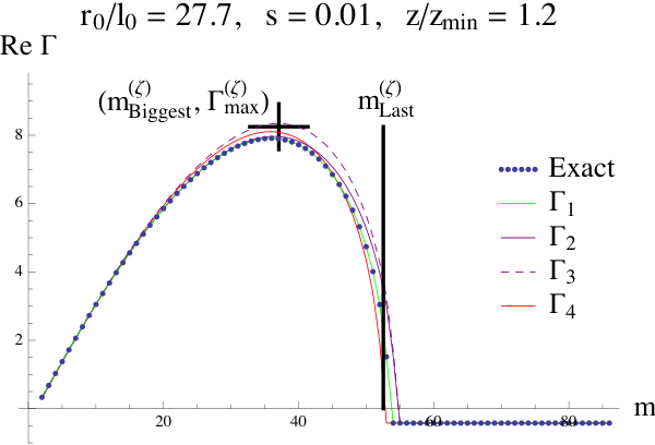
By solving at fixed and , we can extract an estimate of the last unstable mode:
|
|
(55) |
and by solving at fixed and , we can extract an estimate of the most unstable mode:
|
|
(56) |
Here is the lower branch of the Lambert function, which takes values between and for . Thus far we have not required parametrically close to ; however, in order for the estimate in (54) to make sense, we should have
|
|
(57) |
since for larger the estimate (55) breaks down on account of becoming complex when its argument is less than . It is observed that the estimate in (49) works fairly well over a much broader range, for as large as and/or as large as .33 3 An interesting phenomenon captured correctly by at larger values of and is that there can be two disjoint regions of instability, one at small and another at comparable to the location of the single vortex instability as indicated in (24)-(25). As time progresses, these two regions broaden and merge, and at late times one enters the regime well described by the estimate.
If we add the assumption that is close to , then the argument of is small, and we may approximate
|
|
(58) |
The last term in (58), as well as additional corrections to (58), vanish in the limit . Using (58), we find
|
|
(59) |
where
|
|
(60) |
is a positive number which slowly grows large as . With a little more work, one can show that the maximum value of can be approximated as
|
|
(61) |
Our main qualitative conclusions follow from (59) and (61):
- •
The most unstable mode at late times, when is close to has reduced wavelength significantly greater than . More precisely:
(62) The trend of this expression as from above is dominated by the ; in other words, by approximately this factor. This is in contrast to the single vortex instability, where according to (25) by only an factor.
- •
The most unstable mode can be very unstable, due to the dependence in . The strongest dependence in comes from its behaving approximately as . For a fixed initial radius , one can show starting from (40) that
(63) The instability is strongest, then, when . It is almost completely absent for only slightly larger than . At very late times, the factor in (61) written in terms of suppresses the instability, even for large ; however this happens very slowly. The example in figure 2 makes it clear that an unremarkable choice of parameters leads to significantly larger than .
It should be noted that this late-time analysis controls the dominant instability only in a limit where the initial perturbations are sufficiently small. Numerical exploration of (44) indicates that perturbations with finite though small amplitude may grow large before one reaches the asymptotic regime with close to .
4 Derivation of the effective string action
Although well-established (e.g. in [15, 16, 18], an effective description of the dynamics of superfluids in terms of effective strings coupled to a Neveu-Schwarz two-form gauge potential is crucial to our analysis, and it is therefore worth reviewing here, along the lines of [16].
One standard starting point for describing the collective dynamics of a superfluid is the Gross-Pitaevskii lagrangian,
|
|
(64) |
The symmetry is spontaneously broken:
|
|
(65) |
where and is a Goldstone boson. Then
|
|
(66) |
where
|
|
(67) |
The first step is to dualize to . For simplicity, we first treat (66) under the assumption that takes values in rather than : This amounts to omitting the strings. Let us introduce a four-vector , where are auxiliary fields over which we integrate. It is easily verified that
|
|
(68) |
Thus
|
|
(69) |
where we have defined the measure and contour so that
|
|
(70) |
The requirement (70) is troublesome because the result of the Gaussian integration depends on , which is a fluctuating field. We must assume that is a good enough approximation (away from vortices) that (70) can be enforced; in other words, additional terms from relaxing (70) to include dependence are ignored.
Our next step is to perform the path integral over . The first term on the right hand side of (68) may be integrated by parts, so that the path integration over simply enforces the constraint
|
|
(71) |
We solve (71) by setting
|
|
(72) |
where . The reason that (72) works is that (71) is implied by the equality of mixed partials acting on . (72) means in particular that
|
|
(73) |
This is the electric part of the standard action for . To get the rest of the action, we note that
|
|
(74) |
where we have split
|
|
(75) |
and set
|
|
(76) |
with all other components of vanishing except the ones related to (76) by index permutation. Our convention in (74) and elsewhere is to sum over indices without restriction. We can still set , and we split . To summarize, is the background superfluid density, and describes density fluctuations around it, and (nearly) the whole claim is
|
|
(77) |
where and
|
|
(78) |
We now drop the term because it affects the dispersion relation only in the UV:
|
|
(79) |
where is a factor of order unity, and
|
|
(80) |
is the Gross-Pitaevskii coherence length, which is also the approximate radius of a vortex core. In writing (77) we have on the right hand side replaced so that the final theory of excitations is free. Interactions with variable could be developed perturbatively. Note also that we are assuming that the Jacobian between and the natural measure for the two-form gauge field can be neglected. Of course, to properly describe the path integral over , one must develop some sort of gauge-fixing technology.
The main way in which (77) is incomplete is that we ignored the possibility of vortices, around which one has a winding of the phase, . Restricting ourselves for simplicity to a single vortex whose spacetime embedding is , one can show that
|
|
(81) |
For any fixed string configuration , we can split
|
|
(82) |
where satisfies (81) and is a smooth function (i.e. satisfying ). Then
|
|
(83) |
Inside the path integral, the second term in (83) can be integrated by parts, and can be treated as the lagrangian multiplier enforcing the constraint . Upon doing this, we may employ (72) to write
|
|
(84) |
where in the second step we dropped a total derivative. Finally, we integrate over :
|
|
(85) |
which is the desired form, with
|
|
(86) |
An additional aspect of vortex dynamics is that the core has some energy cost per unit length. Without entering into detail, we parametrize this microscopic dynamics by the tension term appearing in (1). Putting this tension term together with (77) and (85), we find the effective action
|
|
(87) |
where . Already to write the tension term we have assumed that the speed of all parts of the vortex is much less than ; otherwise we would need the full Nambu action or some generalization thereof. In order to obtain the action (1) which we use in actual calculations, we must integrate out , using again the quasi-static approximation for the motion of the vortices. An efficient means of doing so is to re-introduce the spacetime vortex current
|
|
(88) |
This current already appeared in (81). Omitting the coupling to the background field , the relevant terms in (87) are
|
|
(89) |
To integrate out we must include some gauge-fixing terms. A convenient choice for present purposes is to require
|
|
(90) |
where runs from to and runs from to . Recalling , we see that
|
|
(91) |
where the gauge condition (90) has been used in the second equality.
For static strings, the only non-vanishing components of are . We therefore consider the combination
|
|
(92) |
where is the laplacian on . Integrating out enables us to drop the first term in square brackets in the last expression in (92); or in the classical theory, we would set
|
|
(93) |
where we have noted that
|
|
(94) |
Thus we arrive at
|
|
(95) |
where to obtain the second line we have parametrized strings in static gauge, so that and with ; thus
|
|
(96) |
The above treatment is complete for truly static strings, where all time dependence is trivial, and the field decouples because . For quasi-static strings, moving much slower than the speed , is a small but non-vanishing source for , and the correct treatment of (87) is
|
|
(97) |
In other words, we have quasi-static strings interacting Coulombically with one another and coupled to a phonon field. Returning to (1), we see that the match with the first two lines of (97) is precise once we identify in (1) as the background field and set
|
|
(98) |
where in the second equality we used (86) and in the third we used (78). Note that upon use of (7) we obtain
|
|
(99) |
As a consistency check, we can inquire whether the motion of vortices as determined through a classical treatment of (1) is indeed much less than . Referring to (21) and (78), we find
|
|
(100) |
which is indeed much less than provided . On the other hand, (43) shows that the expansion that follows head-on vortex collision proceeds at a speed comparable to
|
|
(101) |
In a Gross-Pitaevskii treatment,
|
|
(102) |
is not small: indeed, the study [23] shows that is moderately larger than , not smaller. To justify in detail the treatment of section 3, we must assume that we can arrange ; then among other nice properties, the motion of vortices is uniformly less than , provided only
|
|
(103) |
This last estimate follows from combining (100) with the requirement .
5 Discussion
The action (1) is an efficient description of interacting vortices because fluctuations in the two-form gauge field that mediate the interactions have already been integrated out. The bilocal interaction term in (1) is complicated for general vortex configurations, but for the specific cases of a single vortex and two identical vortices colliding, this bilocal term leads to the impressive series of elliptic integrals which supplied us with many exact or nearly exact results, such as (18) and (51). From a physical perspective, the necessity of cutting off this term provides a notion of renormalization which we have addressed at an elementary level around (20). A more sophisticated effective field theory treatment, including a renormalization group equation for the string tension, can be given, but we will not develop it explicitly here; see however [24]. A key qualitative feature is that the running tension vanishes at length scales comparable to the scale introduced in (20). It is natural to expect the system to do interesting things around this dynamically generated length scale. Indeed, (25) indicates that the single vortex instability occurs at wavelengths only moderately larger than ; and according to (21), retrograde motion of small circular vortex loops occurs for .
In our treatment, we have emphasized that the UV cutoff and the dynamically generated length scale are independent quantities, and one may arrange to have if the rescaled tension is negative. There are reasons to deprecate such an approach. First: several microscopic models of vortex rings were reviewed in [9], and in all cases by a factor of at least (see Table 1 of [9]). Second: The classical energy (26) is negative for , so unless the classical theory has a stability problem. Observing that the quantum zero point energy is positive, one might hold out the hope that quantum effects rescue stability even if ; but if this happens, then quantum effects are very important near and we would have to ask what justifies use of the classical theory to describe fluctuations around this scale. Third: Experimental results on single vortices [10] suggest that finite core size is important in a quantitatively accurate description of the instabilities, and descriptions of colliding vortices often assume significant deformation of the core, as reviewed for example in [8]. Altogether, real-world applications of vortex ring theory seem to call for a departure from the regime. We should however point out that retrograde motion is a remarkable and important feature of rotons in superfluid helium [25], which is a feature of unperturbed single vortex solutions (21) for . Thus we should not lightly abandon the possibility that dynamics of vortex rings at length scales has physical interest.
In any case, we find a useful starting point because it vastly simplifies the analysis, especially in the case of colliding vortices, while retaining many of the key features, in particular the one and two vortex instabilities. Moreover, in the regime, these instabilities are amenable to nearly analytical treatment. Indeed, the frequencies (23) of single vortex fluctuations and the more complex account in section 3 of colliding vortices are the main technical results of this paper. In the case of colliding vortices, we saw that the most unstable modes have wavelengths parametrically larger than at late times. So our results in this direction are not wholly dependent on having .
The experimental finding [11] that the collision of two identical vortex rings at high Reynolds number results in production of many small vortex rings has been a touchstone of the field. Analytical treatments of an unperturbed head-on collision, resulting only in radial expansion of the colliding rings, date back as far as [5]. As far as we know, ours is the first detailed analytical study that accounts at least qualitatively for the production of many vortices, provided the initial vortices are much larger in diameter than . Because our study is based on perturbations around the two original colliding vortices, we can only give an account of the first stages of growth of fluctuations in a mode with large . The crucial physics of the later stage is reconnection: The vortex lines must come into contact and effect a change of topology. As far as we can see, this process must be considered in the microscopic theory, and the best we might expect in an effective theory is to parametrize its timescale and its coupling to sound modes.
It may reasonably be asked why experiments such as [11] on normal fluids at high Reynolds number should be compared with a vortex ring setup derived, as we have done in section 4 from an effective Gross-Pitaevskii description of a superfluid. This has been addressed in [26, 9], where it is argued that well outside the vortex core, where the superfluid density is nearly constant and gradients of it are small, the classical Euler equation applies.
Finally, let us point out a close analogy between vortex rings and giant gravitons. The latter subject is part of a theme emphasized in [27, 28, 29] and related works: in non-commutative spaces, characterized by non-zero form fields, the size of strings, or branes, or brane bound states increases with momentum. Consider for example 2-branes in in the presence of spatial four-form field strength:
|
|
(104) |
To make contact with previous results, let us write and choose a gauge such that
|
|
(105) |
Consider now a 2-brane in the shape of an in the -- plane, propagating along the axis. A stationary configuration can be found by assuming that only depends on time, so that the standard action for a two-brane,
|
|
(106) |
can be written as where
|
|
(107) |
and we are setting the speed of light equal to . Evidently, the lagrangian (107) is in close analogy to the free, unperturbed vortex ring lagrangian appearing in the first line of (9): the only substantive difference is the inertial term in (107). Furthermore, the 2-brane construction we have just discussed can be embedded in the background of M-theory. This was discussed in detail in [29]; to connect (107) to their work, we need only make the identifications
|
|
(108) |
Then in the limit with and held fixed, the lagrangian from (3.14) and (3.18) of [29] precisely matches (107). Physically, we are permitting motions only on the part of the geometry; we are keeping only the time direction out of in the description of the classical motion; and we are keeping the size of the giant graviton fixed while taking the flat space limit in which the number of flux quanta supporting is large. Giant gravitons in are stable because they are BPS. Stability of classical spherical membranes following the dynamics of (106) in flat seems closely related, but as we have seen for a single vortex ring, stability depends on the precise properties of the construction in question.
It would be interesting to develop a similar embedding of (9) into string theory in a flat space limit of a background with non-zero , for example the NS5-brane. However, we do not at present understand how to handle the linear dilaton factor in this geometry. It would also be interesting to inquire how far one can get in describing fluctuations of M2-branes in a limit where second time derivatives are neglected. Generally speaking, quantum fluctuations of M2-branes are a thorny problem, but perhaps progress can be made in some novel non-relativistic limit.
Acknowledgments
We are particularly grateful to B. Horn, A. Nicolis, and R. Penco for stimulating discussions and for insight on the effective field theory aspects of vortex dynamics. This work was supported in part by the Department of Energy under Grant No. DE-FG02-91ER40671.
Appendix A Comparison with a vortex filament calculation
The stability analysis for a single vortex presented in section 2 reproduces the results from [10] to great analytical and numerical accuracy. Table (1) presents the dictionary for translating between our work and that of [10].
| Widnall et al. ’73 [10] | Present work | |
|---|---|---|
| ( Vortex core radius44 4 This, more precisely , is a formal translation between [10] and the present work. The vertex core radius in the present work is in fact of the order of the UV-cutoff . | ||
| ( Vortex ring unperturbed radius | ||
| ( UV-cutoff55 5 The r.h.s in both cells describes the relation between the different length scales in the respective papers, but is not part of the dictionary. | ||
| ( Vortex ring axial velocity | ||
| ( Amplification rate | ||
| ( Radial perturbation | ||
| ( Axial perturbation | ||
| ( Vortex strength | ||
| ( Linearized equations | equations (22) |
Figure 3 in [10] plots the “non-dimensional spatial amplification rate” as a function of another dimensionless quantity , which is proportional to the axial velocity of the unperturbed vortex, where these quantities are defined to be
|
|
(109) |
Using the dictionary, one finds
|
|
(110) |
On plotting versus after substituting for the velocity and exact mode frequencies in (110) by their expressions in (21) and (23), we observe our result: Figure 3 matches the “constant-core-radius” model of [10] exceedingly well, with the exception that in [10] an overlap between the and instabilities was not seen.
As another example, at large the analogs of (22), corresponding to expressions for and , were derived in [10] to be
|
|
(111) |
In our analysis, the corresponding quantities, and are known exactly for any , and can be read off of (22). At large , they become
|
|
(112) |
where we have written and in such a manner so as to make the dictionary between the hydrodynamics treatment [10] and our calculation explicit. The results match up to discrepancies.
We will now derive analytical expressions for the “instability band” and the “maximum amplification rate” as a function of large mode number , closely following the calculation in [10]. In figure 3, the “instability band” corresponds to the lower and upper limits on which yield an instability for mode , while the “maximum amplification rate” corresponds to the maximum at that mode , corresponding to maximum instability. As can be seen in figure 4 which shows the result of this computation, the large approximation works well even at moderate values of (such as 8). The main difference between our computation and that in [10] is that we keep terms in our analysis. The calculation proceeds as follows.
The upper limit for the instability band is obtained by setting in (112), solving for , and substituting the result into (110) to obtain :
|
|
(113) |
The lower limit for the instability band is obtained by setting in (112), expanded about for small , to zero and solving for :
|
|
(114) |
Maximum amplification occurs approximately in the middle of the band, corresponding to
|
|
(115) |
where is given by (113). The corresponding amplification rate can be computed by substituting (115) into (110), and expanding to at large ,
|
|
(116) |
where
|
|
(117) |
In contrast, the authors in [10] obtained which is accurate only at very large , but noted that a better fit to their numerical results was given by
|
|
(118) |
which closely matches our result (116) obtained analytically. In figure 4 we superimposed as obtained in (116) and at the radius of maximum instability (115), as quoted in (117), on the exact result shown in figure 3. As can be seen, the large approximation works very well even for as low as .
References
- [1] S. Endlich and A. Nicolis, “The incompressible fluid revisited: vortex-sound interactions,” 1303.3289.
- [2] H. B. Nielsen and P. Olesen, “Vortex Line Models for Dual Strings,” Nucl.Phys. B61 (1973) 45–61.
- [3] M. Kalb and P. Ramond, “Classical direct interstring action,” Phys.Rev. D9 (1974) 2273–2284.
- [4] F. Lund and T. Regge, “Unified Approach to Strings and Vortices with Soliton Solutions,” Phys.Rev. D14 (1976) 1524.
- [5] F. W. Dyson, “The potential of an anchor ring – Part II,” Philosophical Transactions of the Royal Society of London A184 (1893) 1041–1106.
- [6] K. Shariff and A. Leonard, “Vortex rings,” Annual Review of Fluid Mechanics 24 (1992) 235–279.
- [7] P. G. Saffman, Vortex dynamics. Cambridge University Press, 1992.
- [8] T. T. Lim and T. B. Nickels, “Vortex rings,” in Fluid Vortices, Volume II (S. I. Green, ed.). Kluwer, 1995.
- [9] C. F. Barenghi and R. J. Donnelly, “Vortex rings in classical and quantum systems,” Fluid Dynamics Research 41 (2009), no. 051401 1–31.
- [10] S. E. Widnall and J. P. Sullivan, “On the Stability of Vortex Rings,” Proceedings of the Royal Society of London A332 (1973) 335–353.
- [11] T. T. Lim and T. B. Nickels, “Instability and reconnection in the head-on collision of two vortex rings,” Nature 357 (May, 1992) 225–227.
- [12] D. W. Moore and P. G. Saffman, “A Note on the Stability of a Vortex Ring of Small Cross-Section,” Proceedings of the Royal Society of London A338 (1974) 535–537.
- [13] S. E. Widnall and C.-Y. Tsai, “The Instability of the Thin Vortex Ring of Constant Vorticity,” Philosophical Transactions of the Royal Society of London A287 (1977) 273–305.
- [14] P. G. Saffman, “The number of waves on unstable vortex rings,” Journal of Fluid Mechanics (1978), no. 84 625–639.
- [15] R. L. Davis and E. P. S. Shellard, “Global Strings and Superfluid Vortices,” Physical Review Letters 63 (1989) 2021–2024.
- [16] A. Zee, “Vortex strings and the antisymmetric gauge potential,” Nucl.Phys. B421 (1994) 111–124.
- [17] E. Witten, “Cosmic Superstrings,” Physics Letters B (1985), no. 153 243–246.
- [18] M. Franz, “Vortex-boson duality in four space-time dimensions,” cond-mat/0607310.
- [19] P. H. Roberts and R. J. Donnelly, “Dynamics of vortex rings,” Physics Letters A31 (1970) 137–138.
- [20] M. Luscher, “Symmetry Breaking Aspects of the Roughening Transition in Gauge Theories,” Nucl.Phys. B180 (1981) 317.
- [21] O. Alvarez, “The Static Potential in String Models,” Phys.Rev. D24 (1981) 440.
- [22] K. Shariff, A. Leonard, and J. H. Ferziger, “Dynamics of a Class of Vortex Rings,” Tech. Rep. Technical Memorandum 102257, NASA, 1989.
- [23] P. H. Roberts and J. Grant, “Motions in a Bose condensate. I. The structure of the large circular vortex,” Journal of Physics A: General Physics 4 (1971) 55.
- [24] B. Horn, A. Nicolis, and R. Penco. Forthcoming.
- [25] M. A. H. Tucker and A. F. G. Wyatt, “Direct Evidence for R− Rotons Having Antiparallel Momentum and Velocity,” Science 283 (1999) 1150–1152, http://www.sciencemag.org/content/283/5405/1150.full.pdf.
- [26] C. F. Barenghi, “Is the Reynolds number infinite in superfluid turbulence?,” Physica D237 (2008) 2195–2202.
- [27] D. Bigatti and L. Susskind, “Magnetic fields, branes and noncommutative geometry,” Phys.Rev. D62 (2000) 066004, hep-th/9908056.
- [28] R. C. Myers, “Dielectric branes,” JHEP 9912 (1999) 022, hep-th/9910053.
- [29] J. McGreevy, L. Susskind, and N. Toumbas, “Invasion of the giant gravitons from Anti-de Sitter space,” JHEP 0006 (2000) 008, hep-th/0003075.