跳到论文正文
W Papers独立论文阅读器 arXiv:1408.2207 论文正文 计算阅读时间 · 0%
引用这篇论文根据当前论文元数据生成,正式投稿前建议核对。


License: arXiv.org perpetual non-exclusive license
arXiv:1408.2207v1 [math.NA] 10 Aug 2014

A new operational matrix based on Bernoulli polynomials

Journal: .
J.A. Rad Email: j.amanirad@gmail.com;j_amanirad@sbu.ac.ir Corresponding author: Corresponding author Address: Department of Computer Sciences, Faculty of Mathematical Sciences, Shahid Beheshti University, Evin, P.O. Box 198396-3113,Tehran,Iran    S. Kazem Address: Department of Applied Mathematics, Faculty of Mathematics and Computer Science, Amirkabir University of Technology, No. 424, Hafez Ave., 15914, Tehran, Iran    M. Shaban Address: Department of Scientific Computing, Florida State University, 400 Dirac Science Library, Tallahassee, FL 32306, USA    K. Parand Email: k_parand@sbu.ac.ir Address: Department of Computer Sciences, Faculty of Mathematical Sciences, Shahid Beheshti University, Evin, P.O. Box 198396-3113,Tehran,Iran
Abstract

In this research, the Bernoulli polynomials are introduced. The properties of these polynomials are employed to construct the operational matrices of integration together with the derivative and product. These properties are then utilized to transform the differential equation to a matrix equation which corresponds to a system of algebraic equations with unknown Bernoulli coefficients. This method can be used for many problems such as differential equations, integral equations and so on. Numerical examples show the method is computationally simple and also illustrate the efficiency and accuracy of the method.

Keywords: 
Bernoulli polynomial; Operational matrix; Galerkin method.
AMS subject classification: 65M70, 65L60.

1 Introduction

Differential equations and their solutions play a major role in science and engineering. A physical event can be modeled by the differential equation, an integral equation or an integro-differential equation or a system of these equations. Since few of these equations cannot be solved explicitly, it is often necessary to resort to the numerical techniques which are appropriate combinations of numerical integration and interpolation. The solution of this equations occurring in physics, biology and engineering are based on numerical methods such as the Runge-Kutta methods. In recent years, the differential, integral and integro-differential equations have been solved using the homotopy perturbation method [1, 2], the radial basis functions method [3], the collocation method [4], the Homotopy analysis method [5, 6], the Tau method [7, 8], the Variational iteration method [9, 10], the Legendre matrix method [11, 12], the Haar Wavelets operational matrix [13], the Shifted Chebyshev direct method [14], the Legendre Wavelets operational matrix [15], Sine-Cosine Wavelets operational matrix [16], the operational matrices of Bernstein polynomials [17] and so on.
Polynomial series and orthogonal functions have received considerable attention in dealing with various problems of differential, integral and integro-differential equations. Polynomials are incredibly useful mathematical tools as they are simply defined, can be calculated quickly on computer systems and represent a tremendous variety of functions. They can be differentiated and integrated easily, and can be pieced together to form spline curves that can approximate any function to any accuracy desired. Also, the main characteristic of this technique is that it reduces these problems to those of solving a system of algebraic equations, thus greatly simplifies the problems.
Bernoulli polynomials play an important role in various expansions and approximation formulas which are useful both in analytic theory of numbers and in classical and numerical analysis. The Bernoulli polynomials and numbers have been generalized by Norlund [18] to the Bernoulli polynomials and numbers of higher order. Also, Vandiver in [19] generalized the Bernoulli numbers. Analogous polynomials and sets of numbers have been defined from time to time, witness the Euler polynomials and numbers and the so-called Bernoulli polynomials of the second kind. These polynomials can be defined by various methods depending on the applications [20, 21, 22, 23, 24, 25, 26].
In this paper, the Galerkin method [27] based on operational matrices of integration, differentiation and product for the Bernoulli polynomials are presented.

The remainder of this paper is organized as follows: In Section 2, we describe the basic formulation of Bernoulli polynomials required for our subsequent development. Section 3 is devoted to the function approximation by using this polynomials basis. In Sections 4, we explain general procedure of forming of operational matrices of integration, differentiation and product. In Section 5, we report our numerical findings and demonstrate the validity, accuracy and applicability of the operational matrices by considering numerical examples. Also a conclusion is given in the last Section.

2 Bernoulli polynomials

The classical Bernoulli polynomials of nn-th degree are defined on the interval [0, 1] as

Bn​(x)=∑k=0n(nk)​Bk​xn−k,\displaystyle B_{n}(x)=\sum_{k=0}^{n}{n\choose k}B_{k}x^{n-k}~,

where Bk:=Bk​(0)B_{k}:=B_{k}(0) is the Bernoulli number for each k=0,1,…,nk=0,1,...,n. Thus, the first four such polynomial, respectively, are

B0​(x)=1,B1​(x)=x−12,\displaystyle B_{0}(x)=1~,~~~~~~~~~~~~~~~~B_{1}(x)=x-\frac{1}{2}~,
B2​(x)=x2−x+16,B3​(x)=x3−32​x2+12​x,\displaystyle B_{2}(x)=x^{2}-x+\frac{1}{6}~,~~~B_{3}(x)=x^{3}-\frac{3}{2}x^{2}+\frac{1}{2}x~,

Leopold Kronecker expressed the Bernoulli number BnB_{n} in the following form

Bn=−∑k=1n+1(−1)kk(n+1k)∑j=1kjn,\displaystyle B_{n}=-\sum_{k=1}^{n+1}\frac{(-1)^{k}}{k}{n+1\choose k}\sum_{j=1}^{k}j^{n}~,

for n≥0,n≠1n\geq 0~,~~n\neq 1. If n=1n=1, we defined B1=−12B_{1}=-\frac{1}{2}.
Determinant form of the Bernoulli polynomial of nn-th degree is defined by F. Costabile [28]

B0​(x)=1,\displaystyle B_{0}(x)=1~,

and

Bn​(x)=(−1)n(n−1)!\displaystyle B_{n}(x)=\frac{(-1)^{n}}{(n-1)!} |1xx2x3…xn−1xn1121314…1n1n+10111…110023…n−1n000(32)…(n−12)(n2)⋮⋮⋮⋮⋱⋮⋮0000…(n−1n−2)(nn−2)|.\displaystyle\left|\begin{array}[]{ccccccc}1&x&x^{2}&x^{3}&\dots&x^{n-1}&x^{n}\\ 1&\frac{1}{2}&\frac{1}{3}&\frac{1}{4}&\dots&\frac{1}{n}&\frac{1}{n+1}\\ 0&1&1&1&\dots&1&1\\ 0&0&2&3&\dots&n-1&n\\ 0&0&0&{3\choose 2}&\dots&{n-1\choose 2}&{n\choose 2}\\ \vdots&\vdots&\vdots&\vdots&\ddots&\vdots&\vdots\\ 0&0&0&0&\dots&{n-1\choose n-2}&{n\choose n-2}\\ \end{array}\right|~.

for each n=1,2,…n=1,2,...~.
The Bernoulli polynomials play an important role in different areas of mathematics, including number theory and the theory of finite differences. This polynomial have many similar properties. These polynomials produce the following exponential generating function

t​ex​tet−1=∑n=0∞Bn​(x)​tnn!,\displaystyle\frac{te^{xt}}{e^{t}-1}=\sum_{n=0}^{\infty}B_{n}(x)\frac{t^{n}}{n!}~, (2.8)

Since they satisfy the well-known relation

dd​x​Bn​(x)=n​Bn−1​(x),\displaystyle\frac{d}{dx}B_{n}(x)=nB_{n-1}(x)~, (2.9)

(for all n≥1n\geq 1), which follows easily from Eq. (2.8), it is to be expected that integrals figure prominently in the study of these polynomials. The most immediate integral formula is obtained by integrating Eq. (2.9)

Bn​(x)=n​∫0xBn−1​(t)​𝑑t+Bn,\displaystyle B_{n}(x)=n~\int_{0}^{x}B_{n-1}(t)~dt+B_{n}~, (2.10)

One the other of these properties is

Bn​(x+1)−Bn​(x)=n​xn−1,\displaystyle B_{n}(x+1)-B_{n}(x)=nx^{n-1}~, (2.11)
Bn​(x+1)=∑k=0n(nk)​Bk​(x),\displaystyle B_{n}(x+1)=\sum_{k=0}^{n}{n\choose k}B_{k}(x)~, (2.12)
Bn​(1−x)=(−1)n​Bn​(x),\displaystyle B_{n}(1-x)=(-1)^{n}B_{n}(x)~,
(−1)n​Bn​(−x)=Bn​(x)+n​xn−1,\displaystyle(-1)^{n}B_{n}(-x)=B_{n}(x)+nx^{n-1}~,
∫01Bn​(x)​𝑑x=0,n≥1.\displaystyle\int_{0}^{1}B_{n}(x)~dx=0~,~~~n\geq 1~.

From Eq. (2.11) and (2.12), we obtain for any integer n≥0n\geq 0,

∑k=0n(n+1k)​Bk​(x)=(n+1)​xn.\displaystyle\sum_{k=0}^{n}{n+1\choose k}B_{k}(x)=(n+1)x^{n}~. (2.13)

Also the following interesting integral for a product of two Bernoulli polynomials appears in the book by Nörlund for all k+m≥2k+m\geq 2,

∫01Bn​(t)​Bm​(t)​𝑑t=(−1)n−1​m!​n!(m+n)!​Bn+m.\displaystyle\int_{0}^{1}B_{n}(t)B_{m}(t)~dt=(-1)^{n-1}\frac{m!n!}{(m+n)!}B_{n+m}~. (2.14)

It can be easily shown that any given polynomial of degree nn can be expanded in terms of linear combination of the basis functions

P⁡(x)=∑i=0nCi​Bi​(x)=CT​𝐁​(x),\displaystyle P(x)=\sum_{i=0}^{n}C_{i}B_{i}(x)=C^{T}\mathbf{B}(x)~, (2.15)

where CC and 𝐁⁡(x)\mathbf{B}(x) are (n+1)×1(n+1)\times 1 vectors given by

C=[C0,C1,…,Cn]T,\displaystyle C=[C_{0},C_{1},...,C_{n}]^{T},
𝐁⁡(x)=[B0​(x),B1​(x),…,Bn​(x)]T.\displaystyle\mathbf{B}(x)=[B_{0}(x),B_{1}(x),...,B_{n}(x)]^{T}~. (2.16)

For each i=0,1,…,ni=0,1,...,n~, we can obtain the following matrix form of Bi​(x)B_{i}(x)

Bi​(x)=∑k=0i(ik)​Bk​xi−k\displaystyle B_{i}(x)=\sum_{k=0}^{i}{i\choose k}B_{k}x^{i-k}
=(ii)​Bi+(ii−1)​Bi−1​x+…+(i1)​B1​xi−1+(i0)​B0​xi\displaystyle={i\choose i}B_{i}+{i\choose i-1}B_{i-1}x+...+{i\choose 1}B_{1}x^{i-1}+{i\choose 0}B_{0}x^{i}
=[(ii)​Bi(ii−1)​Bi−1(ii−2)​Bi−2…(i1)​B1(i0)​B00​0​…​0​0⏞n−i]​[1xx2⋮xixi+1⋮xn]\displaystyle=\left[\begin{array}[]{ccccccccccc}{i\choose i}B_{i}&{i\choose i-1}B_{i-1}&{i\choose i-2}B_{i-2}&\dots&{i\choose 1}B_{1}&{i\choose 0}B_{0}&\overbrace{0~~0~~\dots~~0~~0}^{n-i}\\ \end{array}\right]~\left[\begin{array}[]{c}1\\ x\\ x^{2}\\ \vdots\\ x^{i}\\ x^{i+1}\\ \vdots\\ x^{n}\end{array}\right]~
=𝐌i​T​(x).\displaystyle=\mathbf{M}_{i}~\mathrm{T}(x)~. (2.27)

where

T⁡(x)=[1​x​x2…xn]T\displaystyle\mathrm{T}(x)=\Bigg[1~~~x~~~x^{2}~~~~...~~~~x^{n}\Bigg]^{T}~

and

𝐌i=[(ii)​Bi(ii−1)​Bi−1(ii−2)​Bi−2…(i1)​B1(i0)​B00​0​…​0​0⏞n−i]T\displaystyle\mathbf{M}_{i}=\left[\begin{array}[]{ccccccccccc}{i\choose i}B_{i}&{i\choose i-1}B_{i-1}&{i\choose i-2}B_{i-2}&\dots&{i\choose 1}B_{1}&{i\choose 0}B_{0}&\overbrace{0~~0~~\dots~~0~~0}^{n-i}\\ \end{array}\right]^{T}~

Now, we can expand the matrix 𝐁⁡(x)=[B0​(x),B1​(x),…,Bn​(x)]T\mathbf{B}(x)=[B_{0}(x),B_{1}(x),...,B_{n}(x)]^{T} as

𝐁⁡(x)=[B0​(x),B1​(x),…,Bn​(x)]T\displaystyle\mathbf{B}(x)=[B_{0}(x),B_{1}(x),...,B_{n}(x)]^{T}
=[𝐌0​T​(x),𝐌1​T​(x),…,𝐌n​T​(x)]T\displaystyle~~~=[\mathbf{M}_{0}~\mathrm{T}(x),\mathbf{M}_{1}~\mathrm{T}(x),...,\mathbf{M}_{n}~\mathrm{T}(x)]^{T}
=[𝐌0,𝐌1,…,𝐌n]T​T​(x)\displaystyle~~~=[\mathbf{M}_{0},\mathbf{M}_{1},...,\mathbf{M}_{n}]^{T}~\mathrm{T}(x)
=[B00000…0(11)​B1(10)​B0000…0(22)​B2(21)​B1(20)​B000…0(33)​B3(32)​B2(31)​B1(30)​B00…0⋮⋮⋮⋮⋮⋱⋮(nn)​Bn(nn−1)​Bn−1(nn−2)​Bn−2(nn−3)​Bn−30…(n0)​B0]​T​(x)\displaystyle~~~=\left[\begin{array}[]{ccccccc}B_{0}&0&0&0&0&\dots&0\\ {1\choose 1}B_{1}&{1\choose 0}B_{0}&0&0&0&\dots&0\\ {2\choose 2}B_{2}&{2\choose 1}B_{1}&{2\choose 0}B_{0}&0&0&\dots&0\\ {3\choose 3}B_{3}&{3\choose 2}B_{2}&{3\choose 1}B_{1}&{3\choose 0}B_{0}&0&\dots&0\\ \vdots&\vdots&\vdots&\vdots&\vdots&\ddots&\vdots\\ {n\choose n}B_{n}&{n\choose n-1}B_{n-1}&{n\choose n-2}B_{n-2}&{n\choose n-3}B_{n-3}&0&\dots&{n\choose 0}B_{0}\\ \end{array}\right]~\mathrm{T}(x)
=𝐌​T​(x)\displaystyle~~~=\mathbf{M}~\mathrm{T}(x) (2.37)

Then, one has

𝐁⁡(x)=𝐌​T​(x),\displaystyle\mathbf{B}(x)=\mathbf{M}~\mathrm{T}(x)~, (2.38)

where 𝐌\mathbf{M} is the (n+1)×(n+1)(n+1)\times(n+1) matrix and

{𝐌}i,j=1n+1={Bi−j​(i−1i−j),i≥j,0,i<j.\displaystyle\{\mathbf{M}\}_{i,j=1}^{n+1}=\begin{cases}B_{i-j}{i-1\choose i-j}~,&i\geq j~,\\ 0~,&i<j~.\end{cases}

Matrix 𝐌\mathbf{M} is an lower triangular matrix and det(𝐌)=1\det(\mathbf{M})=1, so 𝐌\mathbf{M} is an invertible matrix. On the other hand by using Eq.(2.13) we have

∑k=0n(n+1k)​Bk​(x)=(n+1)​xn,\displaystyle\sum_{k=0}^{n}{n+1\choose k}B_{k}(x)=(n+1)x^{n}~,
𝐐𝐁⁡(x)=T⁡(x)⇒𝐁⁡(x)=𝐐−1​T​(x),\displaystyle\mathbf{Q}\mathbf{B}(x)=\mathrm{T}(x)~~~~~\Rightarrow~~~~~\mathbf{B}(x)=\mathbf{Q}^{-1}~\mathrm{T}(x)~, (2.39)

where 𝐐\mathbf{Q} is the (n+1)×(n+1)(n+1)\times(n+1) matrix and

{𝐐}i,j=1n+1={1i​(ij−1),i≥j,0,i<j.\displaystyle\{\mathbf{Q}\}_{i,j=1}^{n+1}=\begin{cases}\frac{1}{i}{i\choose j-1}~,&i\geq j~,\\ 0~,&i<j~.\end{cases}

Matrix 𝐐\mathbf{Q} is an lower triangular matrix and det(𝐐)=1\det(\mathbf{Q})=1, so 𝐐\mathbf{Q} is an invertible matrix. Then from Eqs. (2.38) and (2.39), one has

𝐐−1=𝐌,\displaystyle\mathbf{Q}^{-1}=\mathbf{M}~,

3 Function approximation

Let us define Λ={x|0≤x≤1}\Lambda=\{x|~~0\leq x\leq 1\} and

L2(Λ)={ν:Λ→ℝ|ν~~~~~L^{2}(\Lambda)=\{\nu:\Lambda\rightarrow\mathbb{R}|\nu is measurable and ||ν||2<∞},||\nu||_{2}<\infty\}~,

where

‖ν‖2=(∫01|ν⁡(x)|2​𝑑x)1/2,\displaystyle||\nu||_{2}=\Bigg(\int_{0}^{1}|\nu(x)|^{2}~dx\Bigg)^{1/2}~, (3.1)

is the norm induced by the inner product of the space L2​(Λ)L^{2}(\Lambda),

<u,ν>=∫01u⁡(x)​ν​(x)​𝑑x,\displaystyle<u,\nu>=\int_{0}^{1}u(x)\nu(x)~dx~, (3.2)

Now, we suppose

𝔅N={B0​(x),B1​(x),…,BN​(x)},\displaystyle\mathfrak{B}_{N}=\{B_{0}(x),B_{1}(x),...,B_{N}(x)\}~,

where 𝔅N\mathfrak{B}_{N} is finite dimensional subspace, therefore 𝔅N\mathfrak{B}_{N} is a complete subspace of L2​(Λ)L^{2}(\Lambda).
The interpolating function of a smooth function uu on a finite interval is denoted by ξN​u\xi_{N}u. It is an element of 𝔅N\mathfrak{B}_{N} and

ξN​u=∑k=0Nak​Bk​(x),\displaystyle\xi_{N}u=\sum_{k=0}^{N}a_{k}B_{k}(x)~,

ξN​u\xi_{N}u is the best projection of uu upon 𝔅N\mathfrak{B}_{N} with respect to the inner product Eq. (3.2) and the norm Eq. (3.1). Thus, we have

<ξN​u−u,Bi​(x)>=0,∀Bi​(x)∈𝔅N,\displaystyle<\xi_{N}u-u,B_{i}(x)>=0~,~~~~~~~\forall~~B_{i}(x)\in\mathfrak{B}_{N}~,

or equivalently

ξN​u​(x)=∑i=0Nai​Bi​(x)=AT​𝐁​(x),\displaystyle\xi_{N}u(x)=\sum_{i=0}^{N}a_{i}B_{i}(x)=A^{T}\mathbf{B}(x)~, (3.3)

where AA and 𝐁⁡(x)\mathbf{B}(x) are (N+1)×1(N+1)\times 1 vectors given by

A=[a0,a1,…,aN]T,\displaystyle A=[a_{0},a_{1},...,a_{N}]^{T},
𝐁⁡(x)=[B0​(x),B1​(x),…,BN​(x)]T,\displaystyle\mathbf{B}(x)=[B_{0}(x),B_{1}(x),...,B_{N}(x)]^{T}~, (3.4)

therefore AA can be obtained by

AT=<ξN​u​(x),𝐁T​(x)>​<𝐁⁡(x),𝐁T​(x)>−1,\displaystyle A^{T}=<\xi_{N}u(x),\mathbf{B}^{T}(x)><\mathbf{B}(x),\mathbf{B}^{T}(x)>^{-1}~,

where

<ξN​u​(x),𝐁T​(x)>=∫01ξN​u​(x)​𝐁T​(x)​𝑑x,\displaystyle<\xi_{N}u(x),\mathbf{B}^{T}(x)>=\int_{0}^{1}\xi_{N}u(x)~\mathbf{B}^{T}(x)~dx~,

is an 1×(N+1)1\times(N+1) vector and

𝐃=<𝐁⁡(x),𝐁T​(x)>=∫01𝐁⁡(x)​𝐁T​(x)​𝑑x,\displaystyle\mathbf{D}=<\mathbf{B}(x),\mathbf{B}^{T}(x)>=\int_{0}^{1}\mathbf{B}(x)~\mathbf{B}^{T}(x)~dx~, (3.5)

is an (N+1)×(N+1)(N+1)\times(N+1) matrix and is said dual matrix of 𝐁⁡(x)\mathbf{B}(x). Suppose that 𝐃={di,j}i,j=1N+1\mathbf{D}=\{d_{i,j}\}_{i,j=1}^{N+1}, and by using Eq. (2.14) one has

di,j=∫01Bi​(x)​Bj​(x)​𝑑x=(−1)i−1​i!​j!(i+j)!​Bi+j,\displaystyle d_{i,j}=\int_{0}^{1}B_{i}(x)B_{j}(x)~dx=(-1)^{i-1}\frac{i!j!}{(i+j)!}B_{i+j}~,

which this shows the matrix DD is symmetric and invertible. For example, if N=5N=5, we have

𝐃=[10000001120−1120012520011800−163000−1120018400−1168000−16300121000012520−116800516632]\displaystyle\mathbf{D}=\left[\begin{array}[]{cccccc}1&0&0&0&0&0\\ 0&\frac{1}{12}&0&\frac{-1}{120}&0&\frac{1}{252}\\ 0&0&\frac{1}{180}&0&\frac{-1}{630}&0\\ 0&\frac{-1}{120}&0&\frac{1}{840}&0&\frac{-1}{1680}\\ 0&0&\frac{-1}{630}&0&\frac{1}{2100}&0\\ 0&\frac{1}{252}&0&\frac{-1}{1680}&0&\frac{5}{16632}\\ \end{array}\right]

4 The operational matrix

It is known that operational matrices are employed for solving many engineering and physical problems such as dynamical systems [5], optimal control systems [6–8], robotic systems [9] etc. Furthermore they are used in several areas of numerical analysis, and they hold particular importance in various subjects such as integral equations [10], differential equations [11,12], calculus of variations [13], partial differential equations [14], integro-differential equations [15,16] etc. Also many books and papers have employed the operational matrix for spectral methods [17,18].
Let us start this section by introducing operational matrices. Suppose that

𝐁⁡(x)=[B0​(x),B1​(x),…,BN​(x)]T,\displaystyle\mathbf{B}(x)=[B_{0}(x),B_{1}(x),...,B_{N}(x)]^{T}~,

the matrices 𝒟\mathcal{D} and ℐ\mathcal{I} are named respectively as the operational matrices of derivatives and integrals if and only if

dd​x​𝐁​(x)=𝒟​𝐁​(x),\displaystyle\frac{d}{dx}\mathbf{B}(x)=\mathcal{D}~\mathbf{B}(x)~,
∫0x𝐁⁡(t)​𝑑t≃ℐ​𝐁​(x).\displaystyle\int_{0}^{x}\mathbf{B}(t)~dt\simeq\mathcal{I}~\mathbf{B}(x)~. (4.1)

Furthermore assume C=[c0,c1,…,cN]C=[c_{0},c_{1},...,c_{N}], C~\tilde{C} is named as the operational matrix of the product if and only if

𝐁⁡(x)​𝐁T​(x)​C≃C~​𝐁​(x).\displaystyle\mathbf{B}(x)\mathbf{B}^{T}(x)C\simeq\tilde{C}~\mathbf{B}(x)~.

4.1 Operational matrix of derivative

Theorem 1. Let 𝐁⁡(x)\mathbf{B}(x) be the Bernoulli vector, 𝒟\mathcal{D} is the (N+1)×(N+1)(N+1)\times(N+1) operational matrix of derivatives, then the elements of 𝒟\mathcal{D} are obtained as

{Di,j}i,j=0N={i,i=j+1,0,o​t​h​e​r​w​i​s​e.\displaystyle\{D_{i,j}\}_{i,j=0}^{N}=\begin{cases}i~,&i=j+1~,\\ 0~,&otherwise~.\end{cases}

Proof. By using Eq. (2.9), we have

dd​x​𝐁​(x)=[dd​x​B0​(x),dd​x​B1​(x),…,dd​x​BN​(x)]\displaystyle\frac{d}{dx}\mathbf{B}(x)=\Bigg[\frac{d}{dx}B_{0}(x),\frac{d}{dx}B_{1}(x),...,\frac{d}{dx}B_{N}(x)\Bigg]
=[0,B0​(x),2​B1​(x),3​B2​(x),…,N​BN−1​(x)]\displaystyle~~~~~=\Bigg[0,B_{0}(x),2B_{1}(x),3B_{2}(x),...,NB_{N-1}(x)\Bigg]
=[0000…001000…000200…000030…00⋮⋮⋮⋮⋱⋮⋮0000…N0]​𝐁​(x)=𝒟​𝐁​(x),\displaystyle~~~~~=\left[\begin{array}[]{ccccccc}0&0&0&0&\dots&0&0\\ 1&0&0&0&\dots&0&0\\ 0&2&0&0&\dots&0&0\\ 0&0&3&0&\dots&0&0\\ \vdots&\vdots&\vdots&\vdots&\ddots&\vdots&\vdots\\ 0&0&0&0&\dots&N&0\\ \end{array}\right]~\mathbf{B}(x)=\mathcal{D}~\mathbf{B}(x),

4.2 Operational matrix of integration

Let 𝐁⁡(x)\mathbf{B}(x) be the Bernoulli vector, ℐ\mathcal{I} is the (N+1)×(N+1)(N+1)\times(N+1) operational matrix of integrative, then by using Eq. (2.10)

∫0x𝐁⁡(t)​𝑑t≃ℐ​𝐁​(x).\displaystyle\int_{0}^{x}\mathbf{B}(t)~dt\simeq\mathcal{I}~\mathbf{B}(x)~.
∫0x𝐁⁡(t)​𝑑t=[∫0xB0​(t)​𝑑t∫0xB1​(t)​𝑑t⋮∫0xBN​(t)​𝑑t]=[B1​(x)−B1B2​(x)−B22B3​(x)−B33⋮BN+1​(x)−BN+1N+1],\displaystyle\int_{0}^{x}\mathbf{B}(t)~dt=\left[\begin{array}[]{c}\int_{0}^{x}B_{0}(t)~dt\\ \int_{0}^{x}B_{1}(t)~dt\\ \vdots\\ \int_{0}^{x}B_{N}(t)~dt\\ \end{array}\right]~=\left[\begin{array}[]{c}B_{1}(x)-B_{1}\\ \frac{B_{2}(x)-B_{2}}{2}\\ \frac{B_{3}(x)-B_{3}}{3}\\ \vdots\\ \frac{B_{N+1}(x)-B_{N+1}}{N+1}\\ \end{array}\right]~,

by using expansion of Bi​(x)B_{i}(x), we have

Bi​(x)−Bii=1i​∑k=0i(ik)​Bk​xi−k−1i​Bi\displaystyle\frac{B_{i}(x)-B_{i}}{i}=\frac{1}{i}\sum_{k=0}^{i}{i\choose k}B_{k}x^{i-k}-\frac{1}{i}B_{i}
=1i​(ii−1)​Bi−1​x+1i​(ii−2)​Bi−2​x2+…+1i​(i1)​B1​xi−1+1i​B0​xi\displaystyle=\frac{1}{i}{i\choose i-1}B_{i-1}x+\frac{1}{i}{i\choose i-2}B_{i-2}x^{2}+...+\frac{1}{i}{i\choose 1}B_{1}x^{i-1}+\frac{1}{i}B_{0}x^{i}
=[01i​(ii−1)​Bi−11i​(ii−2)​Bi−2…1i​(i1)​B11i​B00​0​…​0⏟N−i]​T​(x)\displaystyle=\left[\begin{array}[]{cccccccccc}0&\frac{1}{i}{i\choose i-1}B_{i-1}&\frac{1}{i}{i\choose i-2}B_{i-2}&\dots&\frac{1}{i}{i\choose 1}B_{1}&\frac{1}{i}B_{0}&\underbrace{0~~~0~~~\dots~~~0}_{N-i}\\ \end{array}\right]~\mathrm{T}(x)~
=Ui​T​(x)=Ui​𝐐𝐁​(x),\displaystyle=U_{i}~\mathrm{T}(x)=U_{i}\mathbf{Q}\mathbf{B}(x), (4.21)

where i=1,2,…,Ni=1,2,...,N. So, we just need to approximate BN+1​(x)−BN+1N+1\frac{B_{N+1}(x)-B_{N+1}}{N+1}. By using Eq. (3.3), we have

BN+1​(x)−BN+1N+1≃∑j=0Nχj​Bj​(x)=ΞT​𝐁​(x)\displaystyle\frac{B_{N+1}(x)-B_{N+1}}{N+1}\simeq\sum_{j=0}^{N}\chi_{j}B_{j}(x)=\Xi^{T}~\mathbf{B}(x) (4.22)

where

Ξ=[χ0,χ1,…,χN]T,\displaystyle\Xi~=~[\chi_{0},\chi_{1},...,\chi_{N}]^{T}~,

therefore, by substituting Eqs. (4.21) and (4.22) in Eq. (4.2), we have

∫0x𝐁⁡(t)​𝑑t=[U1​𝐐𝐁​(x)U2​𝐐𝐁​(x)⋮UN​𝐐𝐁​(x)ΞT​𝐌​𝐐​𝐁​(x)]=[U1U2⋮UNΞT​𝐌]​𝐐​𝐁​(x)\displaystyle\int_{0}^{x}\mathbf{B}(t)~dt=\left[\begin{array}[]{c}U_{1}\mathbf{Q}\mathbf{B}(x)\\ U_{2}\mathbf{Q}\mathbf{B}(x)\\ \vdots\\ U_{N}\mathbf{Q}\mathbf{B}(x)\\ \Xi^{T}~\mathbf{M}~\mathbf{Q}~\mathbf{B}(x)\end{array}\right]=\left[\begin{array}[]{c}U_{1}\\ U_{2}\\ \vdots\\ U_{N}\\ \Xi^{T}~\mathbf{M}\\ \end{array}\right]~\mathbf{Q}~\mathbf{B}(x)
=𝐔​𝐐⏟ℐ​𝐁​(x)\displaystyle~~~~~~~~~~~~~~=\underbrace{\mathbf{U}~\mathbf{Q}}_{\mathcal{I}}~\mathbf{B}(x) (4.34)
⇒ℐ=𝐔​𝐐\displaystyle~~~~~~~~~~\Rightarrow~~~~~~~~\mathcal{I}=\mathbf{U}~\mathbf{Q}

where

𝐔=[U1U2…UNΞT​𝐌]T,\displaystyle\mathbf{U}=\Bigg[U_{1}~~~~U_{2}~~~~...~~~~U_{N}~~~~\Xi^{T}\mathbf{M}\Bigg]^{T}~,

4.3 Operational matrix of product

The following property of the product of two B-Polynomials vectors will also be applied

𝐁⁡(x)​𝐁T​(x)​C≃𝐂~​𝐁​(x),\displaystyle\mathbf{B}(x)\mathbf{B}^{T}(x)C\simeq\tilde{\mathbf{C}}\mathbf{B}(x)~, (4.35)

where 𝐂~\tilde{\mathbf{C}} is an (N+1)×(N+1)(N+1)\times(N+1) product operational matrix for the vector CC.
Using the transformation Matrices between 𝐁⁡(x)\mathbf{B}(x) and T⁡(x)\mathrm{T}(x) polynomials of the previous section, we have

𝐁⁡(x)​𝐁T​(x)​C=𝐌​T​(x)​TT​(x)​𝐌T​C⏟𝐍\displaystyle\mathbf{B}(x)\mathbf{B}^{T}(x)C=\mathbf{M}~\mathrm{T}(x)\mathrm{T}^{T}(x)~\underbrace{\mathbf{M}^{T}C}_{\mathbf{N}}

Now, we suppose that

T⁡(x)​TT​(x)​𝐍=𝐍~​T​(x),\displaystyle\mathrm{T}(x)\mathrm{T}^{T}(x)~\mathbf{N}=\tilde{\mathbf{N}}~\mathrm{T}(x)~, (4.36)

Then, we have

𝐁⁡(x)​𝐁T​(x)​C=𝐌​𝐍~​T​(x)=𝐌​𝐍~​𝐐⏟𝐂~​𝐁​(x),\displaystyle\mathbf{B}(x)\mathbf{B}^{T}(x)C=\mathbf{M}\tilde{\mathbf{N}}~\mathrm{T}(x)=\underbrace{\mathbf{M}\tilde{\mathbf{N}}~\mathbf{Q}}_{\tilde{\mathbf{C}}}~\mathbf{B}(x)~,
⇒𝐂~=𝐌​𝐍~​𝐐,\displaystyle~~~~~\Rightarrow~~~~~~~\tilde{\mathbf{C}}=\mathbf{M}\tilde{\mathbf{N}}~\mathbf{Q}~,

now in order to achieve 𝐂~\mathbf{\tilde{C}}, it is sufficient to obtain the 𝐍~\tilde{\mathbf{N}}. By using Eq. (4.36), we have

T⁡(x)​TT​(x)​𝐍=[1xx2…xNxx2x3…xN+1x2x3x4…xN+2⋮⋮⋮⋱⋮xNxN+1xN+2…x2​N]​[n0n1n2⋮nN]\displaystyle\mathrm{T}(x)\mathrm{T}^{T}(x)~\mathbf{N}=\left[\begin{array}[]{ccccc}1&x&x^{2}&\dots&x^{N}\\ x&x^{2}&x^{3}&\dots&x^{N+1}\\ x^{2}&x^{3}&x^{4}&\dots&x^{N+2}\\ \vdots&\vdots&\vdots&\ddots&\vdots\\ x^{N}&x^{N+1}&x^{N+2}&\dots&x^{2N}\\ \end{array}\right]\left[\begin{array}[]{c}n_{0}\\ n_{1}\\ n_{2}\\ \vdots\\ n_{N}\\ \end{array}\right]
=[n0n1n2…nN0n0n1…nN−100n0…nN−2⋮⋮⋮⋱⋮000…n0]​[1xx2⋮xN]=𝐍~​T​(x).\displaystyle=\left[\begin{array}[]{ccccc}n_{0}&n_{1}&n_{2}&\dots&n_{N}\\ 0&n_{0}&n_{1}&\dots&n_{N-1}\\ 0&0&n_{0}&\dots&n_{N-2}\\ \vdots&\vdots&\vdots&\ddots&\vdots\\ 0&0&0&\dots&n_{0}\\ \end{array}\right]\left[\begin{array}[]{c}1\\ x\\ x^{2}\\ \vdots\\ x^{N}\\ \end{array}\right]=\tilde{\mathbf{N}}~\mathrm{T}(x)~.

The constructed operational matrices are now used to solve the following examples.

5 Illustrative examples

To illustrate the efficiency of the proposed method in the present paper, several test examples are carried out. The computational results obtained by using this scheme are in excellent agreement with the exact solutions. For these comparisons the root mean square (RMS) error is applied of the form

R​M​S=∑k=1M(y⁡(xk)−yn​(xk))2M,\displaystyle RMS=\sqrt{\frac{\sum_{k=1}^{M}\big(y(x_{k})-y_{n}(x_{k})\big)^{2}}{M}}~,

where y⁡(xk)y(x_{k}) and ym​(xk)y_{m}(x_{k}) are achieved by exact and numerical solution on xkx_{k} and MM is number of test points.

Example 1. We consider the following Bessel differential equation of order zero [29, 30]

x​d2​u​(x)d​x2+d​u​(x)d​x+x​u​(x)=0,\displaystyle x~\frac{d^{2}u(x)}{dx^{2}}+\frac{du(x)}{dx}+x~u(x)=0~, (5.1)

with initial conditions

u⁡(0)=1,d​u​(x)d​x|x=0=0,\displaystyle u(0)=1~,~~~~\frac{du(x)}{dx}\bigg|_{x=0}=0~, (5.2)

The exact solution of this problem is

u⁡(x)=∑i=0∞(−1)i4i​(i!)2​x2​i.\displaystyle u(x)=\sum_{i=0}^{\infty}\frac{(-1)^{i}}{4^{i}(i!)^{2}}x^{2i}~.

To solve this example, we approximate d2​u​(x)/d​x2d^{2}u(x)/dx^{2} by the Bernoulli polynomials as

d2​u​(x)d​x2=AT​𝐁​(x),\displaystyle\frac{d^{2}u(x)}{dx^{2}}=A^{T}\mathbf{B}(x)~,

Also, by using the initial conditions Eq. (5.2) and the operation matrix of integration Eq. (4.1), we have:

d​u​(x)d​x=AT​ℐ​𝐁​(x),\displaystyle\frac{du(x)}{dx}=A^{T}\mathcal{I}\mathbf{B}(x)~,
u⁡(x)=AT​ℐ2​𝐁​(x)+VT​𝐁​(x),\displaystyle u(x)=A^{T}\mathcal{I}^{2}\mathbf{B}(x)+V^{T}\mathbf{B}(x)~, (5.3)

where VT​𝐁​(x)=1V^{T}\mathbf{B}(x)=1 and V=[1,0,0,…,0]TV=[1,0,0,...,0]^{T}. We can express function xx as

x=ET​𝐁​(x),\displaystyle x=E^{T}\mathbf{B}(x)~,

where E=[1/2,1,0,…,0]TE=[1/2,1,0,...,0]^{T}. Therefore, equation (5.1) can be rewrite as:

ET​𝐁​(x)​𝐁T​(x)​A+AT​ℐ​𝐁​(x)+ET​𝐁​(x)​𝐁T​(x)​(ℐ2)T​A+ET​𝐁​(x)​𝐁T​(x)​V=0,\displaystyle E^{T}\mathbf{B}(x)\mathbf{B}^{T}(x)A+A^{T}\mathcal{I}\mathbf{B}(x)+E^{T}\mathbf{B}(x)\mathbf{B}^{T}(x)(\mathcal{I}^{2})^{T}A+E^{T}\mathbf{B}(x)\mathbf{B}^{T}(x)V=0~,

or

(ET​𝐀~+AT​ℐ+ET​𝐙~+ET​𝐕~)​𝐁​(x)=0,\displaystyle\Bigg(E^{T}\tilde{\mathbf{A}}+A^{T}\mathcal{I}+E^{T}\tilde{\mathbf{Z}}+E^{T}\tilde{\mathbf{V}}\Bigg)\mathbf{B}(x)=0~,

where

𝐁⁡(x)​𝐁T​(x)​A=𝐀~​𝐁​(x),\displaystyle\mathbf{B}(x)\mathbf{B}^{T}(x)A=\tilde{\mathbf{A}}\mathbf{B}(x)~,
Z=(ℐ2)T​A,\displaystyle Z=(\mathcal{I}^{2})^{T}A~,
𝐁⁡(x)​𝐁T​(x)​Z=𝐙~​𝐁​(x),\displaystyle\mathbf{B}(x)\mathbf{B}^{T}(x)Z=\tilde{\mathbf{Z}}\mathbf{B}(x)~,
𝐁⁡(x)​𝐁T​(x)​V=𝐕~​𝐁​(x),\displaystyle\mathbf{B}(x)\mathbf{B}^{T}(x)V=\tilde{\mathbf{V}}\mathbf{B}(x)~,

Now, by using Galerkin method [27] and Eq. (3.5), we have

∫01(ET​𝐀~+AT​ℐ+ET​𝐙~+ET​𝐕~)​𝐁​(x)​𝐁​(x)​𝑑x\displaystyle\int_{0}^{1}\Bigg(E^{T}\tilde{\mathbf{A}}+A^{T}\mathcal{I}+E^{T}\tilde{\mathbf{Z}}+E^{T}\tilde{\mathbf{V}}\Bigg)\mathbf{B}(x)\mathbf{B}(x)~dx
=(ET​𝐀~+AT​ℐ+ET​𝐙~+ET​𝐕~)​∫01𝐁⁡(x)​𝐁​(x)​𝑑x\displaystyle=\Bigg(E^{T}\tilde{\mathbf{A}}+A^{T}\mathcal{I}+E^{T}\tilde{\mathbf{Z}}+E^{T}\tilde{\mathbf{V}}\Bigg)\int_{0}^{1}\mathbf{B}(x)\mathbf{B}(x)~dx
=(ET​𝐀~+AT​ℐ+ET​𝐙~+ET​𝐕~)​𝐃=0.\displaystyle=\Bigg(E^{T}\tilde{\mathbf{A}}+A^{T}\mathcal{I}+E^{T}\tilde{\mathbf{Z}}+E^{T}\tilde{\mathbf{V}}\Bigg)\mathbf{D}=0~.

Since 𝐃\mathbf{D} is an invertible matrix, thus one has

ET​𝐀~+AT​ℐ+ET​𝐙~+ET​𝐕~=0.\displaystyle E^{T}\tilde{\mathbf{A}}+A^{T}\mathcal{I}+E^{T}\tilde{\mathbf{Z}}+E^{T}\tilde{\mathbf{V}}=0~.

We generate N+1N+1 equations, therefore by solving above equations the unknown vector AA is achieved and from Eq. (5.3), u⁡(x)u(x) can be calculated.
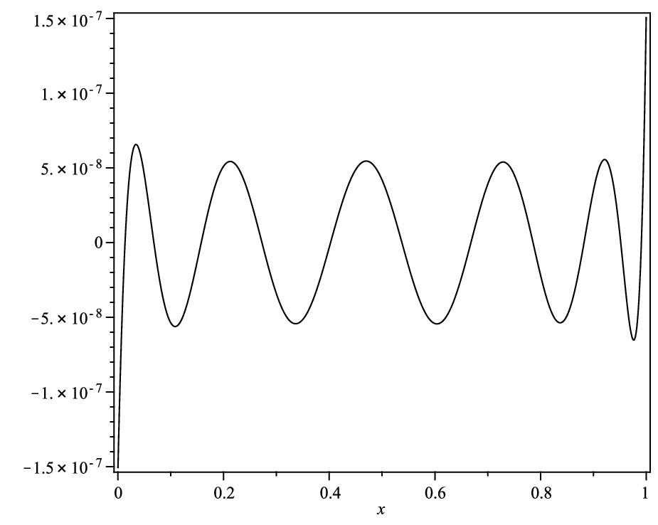
In Table 1, a comparison is made between the approximate values using the present approach together with the exact solution for some various NN. Also, the RMS errors for some various NN are shown in Table 1. From Table 1, it can be seen that a few term of Bernoulli polynomials is sufficient to achieve a good approximation. In Figure 1 the absolute error between the present method and exact solution for N=10N=10 is plotted. Figure 2 represents the coefficients of the Bernoulli polynomials obtained by the present method for some various NN of the Bessel equation. This figure shows that the method has an appropriate convergence rate.

Example 2. In this example we consider the following Lane-Emden type equation [31, 32, 33, 34]

x​d2​u​(x)d​x2+8​d​u​(x)d​x+x2​u​(x)=x6−x5+44​x3−30​x2,\displaystyle x~\frac{d^{2}u(x)}{dx^{2}}+8\frac{du(x)}{dx}+x^{2}~u(x)=x^{6}-x^{5}+44x^{3}-30x^{2}~, (5.4)

with initial conditions

u⁡(0)=0,d​u​(x)d​x|x=0=0,\displaystyle u(0)=0~,~~~~\frac{du(x)}{dx}|_{x=0}=0~, (5.5)

The exact solution of this problem is

u⁡(x)=x4−x3.\displaystyle u(x)=x^{4}-x^{3}~.

Now, we approximate d2​u​(x)/d​x2d^{2}u(x)/dx^{2} by the Bernoulli polynomials as

d2​u​(x)d​x2=AT​𝐁​(x),\displaystyle\frac{d^{2}u(x)}{dx^{2}}=A^{T}\mathbf{B}(x)~,

Also, by using the initial conditions Eq. (5.5) and the operation matrix of integration Eq. (4.1), one has:

d​u​(x)d​x=AT​ℐ​𝐁​(x),\displaystyle\frac{du(x)}{dx}=A^{T}\mathcal{I}\mathbf{B}(x)~,
u⁡(x)=AT​ℐ2​𝐁​(x),\displaystyle u(x)=A^{T}\mathcal{I}^{2}\mathbf{B}(x)~, (5.6)

The functions x,x2,x6−x5+44​x3−30​x2x,~x^{2},~x^{6}-x^{5}+44x^{3}-30x^{2} can be expressed as

x=ET​𝐁​(x),\displaystyle x=E^{T}\mathbf{B}(x)~,
x2=FT​𝐁​(x),\displaystyle x^{2}=F^{T}\mathbf{B}(x)~,
x6−x5+44​x3−30​x2=VT​𝐁​(x),\displaystyle x^{6}-x^{5}+44x^{3}-30x^{2}=V^{T}\mathbf{B}(x)~,

where

E=[1/2,1,0,…,0]T,\displaystyle E=[1/2,~1,~0,...,~0]^{T}~,
F=[1/3,1,1,0,0..,0]T,\displaystyle F=[1/3,~1,~1,~0,~0..,~0]^{T}~,
V=[41/42,14,73/2,137/3,5/2,2,1,0,0,…,0]T.\displaystyle V=[41/42,~14,~73/2,~137/3,~5/2,~2,~1,~0,~0,~...,~0]^{T}.

Therefore, equation (5.4) can be written as:

ET​𝐁​(x)​𝐁T​(x)​A+8​AT​ℐ​𝐁​(x)+FT​𝐁​(x)​𝐁T​(x)​(ℐ2)T​A−VT​𝐁​(x)=0,\displaystyle E^{T}\mathbf{B}(x)\mathbf{B}^{T}(x)A+8A^{T}\mathcal{I}\mathbf{B}(x)+F^{T}\mathbf{B}(x)\mathbf{B}^{T}(x)(\mathcal{I}^{2})^{T}A-V^{T}\mathbf{B}(x)=0~,

or

(ET​𝐀~+8​AT​ℐ+FT​𝐙~−VT)​𝐁​(x)=0,\displaystyle\Bigg(E^{T}\tilde{\mathbf{A}}+8A^{T}\mathcal{I}+F^{T}\tilde{\mathbf{Z}}-V^{T}\Bigg)\mathbf{B}(x)=0~,

where

𝐁⁡(x)​𝐁T​(x)​A=𝐀~​𝐁​(x),\displaystyle\mathbf{B}(x)\mathbf{B}^{T}(x)A=\tilde{\mathbf{A}}\mathbf{B}(x)~,
Z=(ℐ2)T​A,\displaystyle Z=(\mathcal{I}^{2})^{T}A~,
𝐁⁡(x)​𝐁T​(x)​Z=𝐙~​𝐁​(x),\displaystyle\mathbf{B}(x)\mathbf{B}^{T}(x)Z=\tilde{\mathbf{Z}}\mathbf{B}(x)~,

By solving above equation for N=4N=4, we obtain AT=(1,6,12)A^{T}=\big(1,6,12\big). Therefore

d2​u​(x)d​x2=AT​𝐁​(x)=(1,6,12)​(1x−1/2x2−x+1/6)=12​x2−6​x,\displaystyle\frac{d^{2}u(x)}{dx^{2}}=A^{T}\mathbf{B}(x)=\big(1,6,12\big)\left(\begin{array}[]{c}1\\ x-1/2\\ x^{2}-x+1/6\\ \end{array}\right)=12x^{2}-6x~,
d​u​(x)d​x=∫0xd2​u​(t)d​t2​𝑑t=4​x3−3​x2,\displaystyle\frac{du(x)}{dx}=\int_{0}^{x}\frac{d^{2}u(t)}{dt^{2}}dt=4x^{3}-3x^{2}, (5.11)
u⁡(x)=∫0xd​u​(t)d​t​𝑑t=x4−x3,\displaystyle u(x)=\int_{0}^{x}\frac{du(t)}{dt}dt=x^{4}-x^{3},

which is the exact solution of the problem.

Example 3. In this example we consider the following nonlinear Riccati equation [35, 36, 37, 38, 39, 40]

d​u​(x)d​x=2​u​(x)−u2​(x)+1,\displaystyle\frac{du(x)}{dx}=2u(x)-u^{2}(x)+1~, (5.12)

with initial condition

u⁡(0)=0,\displaystyle u(0)=0~, (5.13)

The exact solution of this problem is

u⁡(x)=1+2​tanh⁡(2​x+12​ln⁡(2−12+1)).\displaystyle u(x)=1+\sqrt{2}\tanh\Bigg(\sqrt{2}x+\frac{1}{2}\ln(\frac{\sqrt{2}-1}{\sqrt{2}+1})\Bigg)~.

Now, we approximate d​u​(x)/d​xdu(x)/dx by the Bernoulli polynomials as

d​u​(x)d​x=AT​𝐁​(x),\displaystyle\frac{du(x)}{dx}=A^{T}\mathbf{B}(x)~,

Also, by using the initial conditions Eq. (5.13) and the operation matrix of integration Eq. (4.1), we have:

u⁡(x)=AT​ℐ​𝐁​(x),\displaystyle u(x)=A^{T}\mathcal{I}\mathbf{B}(x)~, (5.14)
u2​(x)=AT​ℐ​𝐁​(x)​𝐁​(x)T​ℐT​A=AT​ℐ​𝐙~​𝐁​(x),\displaystyle u^{2}(x)=A^{T}\mathcal{I}\mathbf{B}(x)\mathbf{B}(x)^{T}\mathcal{I}^{T}A=A^{T}\mathcal{I}\tilde{\mathbf{Z}}\mathbf{B}(x)~, (5.15)

where

Z=ℐT​A,\displaystyle Z=\mathcal{I}^{T}A~,
𝐁⁡(x)​𝐁​(x)T​Z=𝐙~​𝐁​(x).\displaystyle\mathbf{B}(x)\mathbf{B}(x)^{T}Z=\tilde{\mathbf{Z}}\mathbf{B}(x)~.

Therefore, equation (5.12) can be rewritten as:

−AT+2​AT​ℐ−AT​ℐ​𝐙~+ET=0,\displaystyle-A^{T}+2A^{T}\mathcal{I}-A^{T}\mathcal{I}\tilde{\mathbf{Z}}+E^{T}=0~,

where 1=ET​𝐁​(x)1=E^{T}~\mathbf{B}(x).
As in a typical Galerkin method [27] we generate N+1N+1 equations, therefore by solving above equations the unknown vector AA is achieved and the unknown u⁡(x)u(x) can be calculated by using Eq. (5.14).
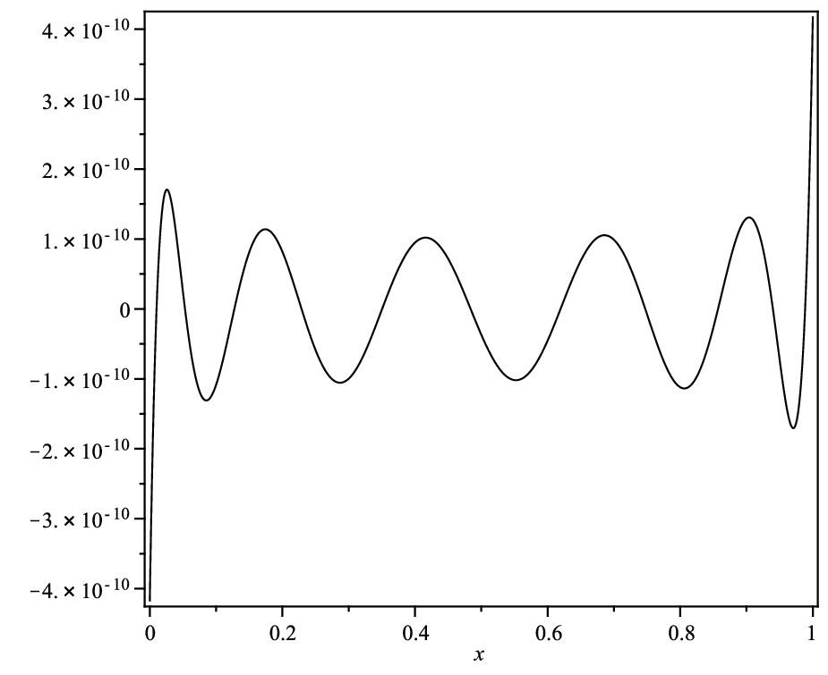
In Table 2, a comparison is made between the approximate values using the introduced technique together with the exact solution for some various NN. Also, the RMS errors for some various NN are shown in Table 2. From Table 2, it can be seen that a few term of Bernoulli polynomials is sufficient to achieve a good approximation. In Figure 3 the absolute error between our obtained approximate solutions and exact solution for N=10N=10 is plotted.

Example 4. Finally, we consider the following nonlinear Riccati equation [39, 40]

d​u​(x)d​x=1+x2−u2​(x),\displaystyle\frac{du(x)}{dx}=1+x^{2}-u^{2}(x)~, (5.16)

with initial condition

u⁡(0)=1,\displaystyle u(0)=1~, (5.17)

and the exact solution of this problem is

u⁡(x)=x+e−x21+∫0xe−t2​𝑑t.\displaystyle u(x)=x+\frac{e^{-x^{2}}}{1+\int_{0}^{x}e^{-t^{2}}~dt}~.

Now, we approximate d​u​(x)/d​xdu(x)/dx by the Bernoulli polynomials as

d​u​(x)d​x=AT​𝐁​(x),\displaystyle\frac{du(x)}{dx}=A^{T}\mathbf{B}(x)~,

Also, by using the initial conditions Eq. (5.13) and the operation matrix of integration Eq. (4.1), one has:

u⁡(x)=AT​ℐ​𝐁​(x)+ET​𝐁​(x),\displaystyle u(x)=A^{T}\mathcal{I}\mathbf{B}(x)+E^{T}\mathbf{B}(x)~, (5.18)
u2​(x)=(AT​ℐ​𝐙~+ET​𝐄~+ET​𝐙~+AT​ℐ​𝐄~)​𝐁​(x),\displaystyle u^{2}(x)=\Bigg(A^{T}\mathcal{I}\tilde{\mathbf{Z}}+E^{T}\tilde{\mathbf{E}}+E^{T}\tilde{\mathbf{Z}}+A^{T}\mathcal{I}\tilde{\mathbf{E}}\Bigg)\mathbf{B}(x)~,

where

Z=ℐT​A,\displaystyle Z=\mathcal{I}^{T}A~,
𝐁⁡(x)​𝐁​(x)T​Z=𝐙~​𝐁​(x),\displaystyle\mathbf{B}(x)\mathbf{B}(x)^{T}Z=\tilde{\mathbf{Z}}\mathbf{B}(x)~,
𝐁⁡(x)​𝐁​(x)T​E=𝐄~​𝐁​(x).\displaystyle\mathbf{B}(x)\mathbf{B}(x)^{T}E=\tilde{\mathbf{E}}\mathbf{B}(x)~.

The function 1+x21+x^{2} is given as

1+x2=FT​𝐁​(x),\displaystyle 1+x^{2}=F^{T}\mathbf{B}(x)~,

where

V=[4/3,1,1,0,0,…,0]T.\displaystyle V=[4/3,~1,~1,~0,~0,~...,~0]^{T}.

Therefore, Eq. (5.16) can be rewritten as:

AT−FT+AT​ℐ​𝐙~+ET​𝐄~+ET​𝐙~+AT​ℐ​𝐄~=0,\displaystyle A^{T}-F^{T}+A^{T}\mathcal{I}\tilde{\mathbf{Z}}+E^{T}\tilde{\mathbf{E}}+E^{T}\tilde{\mathbf{Z}}+A^{T}\mathcal{I}\tilde{\mathbf{E}}=0~,

As in a typical Galerkin method [27] we generate N+1N+1 equations, therefore by solving above equations the unknown vector AA is achieved and the unknown u⁡(x)u(x) can be calculated from Eq. (5.18).
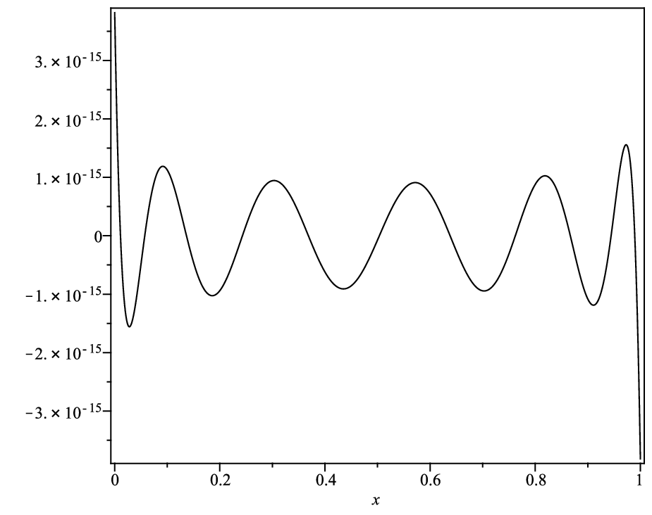
In Table 3, a comparison is made between the approximate values of the applied scheme together with the exact solution for some various NN. Also, the RMS errors for some various NN are shown in Table 3. From Table 3, it can be seen that a few term of Bernoulli polynomials is sufficient to achieve a good approximation. In Figure 4 the absolute error between our approximate results and the exact solution for N=10N=10 is plotted. Figure 5 represents the coefficients of the Bernoulli polynomials obtained by the present method for some various NN of the Bessel equation. This figure shows that the method has an appropriate convergence rate.

6 Conclusions

Nonlinear differential and integral equations have a very important place in physics, mathematics and engineering. Since this equations are usually difficult to solve analytically, it is required to obtain their approximate solution. For this reason, the present method has been proposed to approximate the solutions of these equations using the Bernoulli polynomials. In this paper, the Bernoulli polynomials operational matrices of integration, differentiation and product are derived. A general procedure of forming these matrices are given. The method is general, easy to implement, and yields very accurate results. Moreover, only a few number of basis yields a satisfactory result.

References

  • [1] A. Yildirim, S. Sezer, Y. Kaplan, Analytical approach to Boussinesq equation with space and time-fractional derivatives, Int. J. Numer. Meth. Fluids 66 (2011) 1315–1324.
  • [2] J. H. He, Application of homotopy perturbation method to nonlinear wave equations, Chaos, Solitons and Fractals 26 (2005) 695–700.
  • [3] S. Kazem, J. Rad, K. Parand, Radial basis functions methods for solving Fokker-Planck equation, Eng. Anal. Bound. Elem. (2011), in press.
  • [4] K. Parand, M. Shahini, M. Dehghan, Rational Legendre pseudospectral approach for solving nonlinear differential equations of Lane-Emden type, J. Comput. Phys. 228 (2009) 8830–8840.
  • [5] S. Abbasbandy, E. Shivanian, A new analytical technique to solve Fredholm’s integral equations, Numer. Algorithms 56 (2011) 27–43.
  • [6] S. J. Liao, Series solution of nonlinear eigenvalue problems by means of the homotopy analysis method, Nonlinear Analysis: Real World Applications 10 (2009) 2455–2470.
  • [7] K. Parand, M. Razzaghi, Rational Legendre approximation for solving some physical problems on semi-infinite intervals, Phys. Scr. 69 (2004) 353–357.
  • [8] K. Parand, M. Razzaghi, Rational Chebyshev tau method for solving higher-order ordinary differential equations, Int. J. Comput. Math. 81 (2004) 73–80.
  • [9] S. Yousefi, M. Dehghan, The use of He’s variational iteration method for solving variational problems, Int. J. Comput. Math. 87 (2010) 1299–1314.
  • [10] A. Wazwaz, A reliable treatment of singular Emden-Fowler initial value problems and boundary value problems, Appl. Math. Comput. 217 (2011) 10387–10395.
  • [11] A. Saadatmandi, M. Dehghan, A new operational matrix for solving fractional-order differential equations, Comput. Math. Appl. 59 (2010) 1326–1336.
  • [12] A. Saadatmandi, M. Dehghan, A tau approach for solution of the space fractional diffusion equation, Comput. Math. Appl. (2010) in press.
  • [13] J. S. Gu, W. S. Jiang, The haar wavelets operational matrix of integration, I. J. Syst. Sci. 27 (1996) 623–628.
  • [14] I. Horng, J. Chou, Shifted Chebyshev direct method for solving variational problems, I. J. Syst. Sci. 16 (1985) 855–861.
  • [15] M. Razzaghi, S. Yousefi, The legendre Wavelets operational matrix of integration, I. J. Syst. Sci. 32 (2001) 495–502.
  • [16] M. Razzaghi, S. Yousefi, Sine-Cosine Wavelets operational matrix of integration and its applications in the calculus of variations, I. J. Syst. Sci. 33 (2002) 805–810.
  • [17] S. A. Yousefi, M. Behroozifar, Operational matrices of bernstein polynomials and their applications, I. J. Sys. Sci. 41 (2010) 709–716.
  • [18] N. E. Norlund, Vorlesungen uber Differenzenrechnung, Springer-Verlag, New York, 1954.
  • [19] H. Vandiver, Certain congruences involving the Bernoulli numbers, Duke Mathematical Journal 5 (1939) 548–551.
  • [20] G. Cheon, A note on the Bernoulli and Euler polynomials, Appl. Math. Lett. 16 (2003) 365–368.
  • [21] B. Kurt, Y. Simsek, Notes on generalization of the Bernoulli type polynomials, Appl. Math. Comput. (2011) doi:10.1016/j.amc.2011.03.086.
  • [22] D. Lu, Some properties of Bernoulli polynomials and their generalizations, Appl. Math. Lett. 24 (2011) 746–751.
  • [23] T. Agoh, K. Dilcher, Integrals of products of Bernoulli polynomials, J. Math. Anal. Appl. 381 (2011) 10–16.
  • [24] T. Buric, N. Elezovic, Bernoulli polynomials and asymptotic expansions of the quotient of gamma functions, J. Comput. Appl. Math. 235 (2011) 3315–3331.
  • [25] P. Natalini, A. Bernardini, A generalization of the Bernoulli polynomials, J. Appl. Math. 2003 (2003) 155–163.
  • [26] B. Kurt, A further generalization of the Bernoulli polynomials and on the 2​d2d-Bernoulli polynomials Bn2​(x,y){B}_{n}^{2}(x,y), Appl. Math. Sci. 4 (2010) 2315–2322.
  • [27] D. Gottlieb, M. Hussaini, S. Orszg, Theory and applications of spectral methods in spectral methods for partial differential equations, SIAM, Philadelphia, 1984.
  • [28] F. Costabile, Expansions of real functions in Bernoulli polynomials and applications, Conf. Sem. Mat.Univ. Bari, N. 273 (1999) 1–13.
  • [29] P. O’Neil, Advanced Engineering Mathematics, Belmont, California, 1987.
  • [30] S. Yousefi, M. Behroozifar, Operational matrices of Bernstein polynomials and their applications, I. J. Sys. Sci. 41 (2010) 709–716.
  • [31] J. Ramos, Linearization techniques for singular initial-value problems of ordinary differential equations, Appl. Math. Comput. 161 (2005) 525–542.
  • [32] M. Chowdhury, I. Hashim, Solutions of Emden-Fowler equations by homotopy perturbation method, Nonlinear Anal. Real World Appl. 10 (2009) 104–115.
  • [33] A. Bataineh, M. Noorani, I. Hashim, Homotopy analysis method for singular IVPs of Emden-Fowler type, Commun. Nonlinear Sci. Numer. Simul. 14 (2009) 1121–1131.
  • [34] K. Parand, M. Dehghan, A. Rezaei, S. Ghaderi, An approximation algorithm for the solution of the nonlinear Lane-Emden type equations arising in astrophysics using Hermite functions collocation method, Comput. Phys. Commun. 181 (2010) 1096–1108.
  • [35] M. El-Tawil, A. Bahnasawi, A. Abdel-Naby, Solving Riccati differential equation using Adomian’s decomposition method, Appl. Math. Comput. 157 (2004) 503–514.
  • [36] S. Abbasbandy, Homotopy perturbation method for quadratic Riccati differential equation and comparison with Adomian’s decomposition method, Appl. Math. Comput. 172 (2006) 485–490.
  • [37] S. Abbasbandy, A new application of He’s variational iteration method for quadratic Riccati differential equation by using Adomian’s polynomials, J. Comput. Appl. Math. 207 (2007) 59–63.
  • [38] S. Abbasbandy, Iterated He’s homotopy perturbation method for quadratic Riccati differential equation, Appl. Math. Comput. 175 (2006) 581–589.
  • [39] F. Geng, Y. Lin, M. Cui, A piecewise variational iteration method for Riccati differential equations, Comput. Math. Appl. 58 (2009) 2518–2522.
  • [40] F. Geng, A modified variational iteration method for solving Riccati differential equations, Comput. Math. Appl. 60 (2010) 1868–1872.
Refer to caption
Figure 1: Absolute error function for N=10N=10 in Example 1.
Refer to caption
Figure 2: Absolute values |ai||a_{i}| of the coefficients of the Bernoulli polynomials for some various NN in Example 1.
Refer to caption
Figure 3: Absolute error function for N=10N=10 in Example 3.
Refer to caption
Figure 4: Absolute error function for N=10N=10 in Example 4.
Refer to caption
Figure 5: Absolute values |ai||a_{i}| of the coefficients of the Bernoulli polynomials for some various NN in Example 4.
Table 1: A comparison between the approximate values of the present approach together with the exact solution and the RMS errors for some various NN in Example 1.
  xx Exact N=2N=2 N=4N=4 N=6N=6 N=8N=8 N=10N=10
   0.00.0 1.00000000001.0000000000 1.00147548861.0014754886 0.99999508170.9999950817 1.00000000751.0000000075 1.00000000001.0000000000 1.00000000001.0000000000
   0.20.2 0.99002497220.9900249722 0.98957873970.9895787397 0.99002595660.9900259566 0.99002497470.9900249747 0.99002497220.9900249722 0.99002497220.9900249722
   0.40.4 0.96039822670.9603982267 0.95985676150.9598567615 0.96039656390.9603965639 0.96039822440.9603982244 0.96039822670.9603982267 0.96039822670.9603982267
   0.60.6 0.91200486350.9120048635 0.91230955420.9123095542 0.91200625260.9120062526 0.91200486570.9120048657 0.91200486350.9120048635 0.91200486350.9120048635
   0.80.8 0.84628735270.8462873527 0.84693711760.8469371176 0.84628683780.8462868378 0.84628735030.8462873503 0.84628735270.8462873527 0.84628735270.8462873527
   1.01.0 0.76519768660.7651976866 0.76373945190.7637394519 0.76520259980.7652025998 0.76519767900.7651976790 0.76519768660.7651976866 0.76519768660.7651976866
   RMS −- 7.9298×10−47.9298\times 10^{-4} 2.5651×10−62.5651\times 10^{-6} 3.7742×10−93.7742\times 10^{-9} 3.1762×10−123.1762\times 10^{-12} 1.901×10−151.901\times 10^{-15}
Table 2: A comparison between the approximate values of the present approach together with the exact solution and the RMS errors for some various NN in Example 3.
  xx Exact N=4N=4 N=6N=6 N=8N=8 N=10N=10 N=14N=14
   0.00.0 0.00000000000.0000000000 0.00252650130.0025265013 0.00011285710.0001128571 0.00000448670.0000044867 0.00000000000.0000000000 0.00000000000.0000000000
   0.20.2 0.24197679960.2419767996 0.24127985350.2412798535 0.24194316490.2419431649 0.24197741620.2419774162 0.24197685080.2419768508 0.24197679960.2419767996
   0.40.4 0.56781216630.5678121663 0.56870806280.5687080628 0.56784575620.5678457562 0.56781295860.5678129586 0.56781216310.5678121631 0.56781216620.5678121662
   0.60.6 0.95356621640.9535662164 0.95291919210.9529191921 0.95353372100.9535337210 0.95356482270.9535648227 0.95356616220.9535661622 0.95356621640.9535662164
   0.80.8 1.34636365541.3463636554 1.34659154321.3465915432 1.34640205341.3464020534 1.34636452651.3463645265 1.34636363351.3463636335 1.34636365531.3463636553
   1.01.0 1.68949839161.6894983916 1.68697365611.6869736561 1.68961124631.6896112463 1.68949390491.6894939049 1.68949854271.6894985427 1.68949839161.6894983916
   RMS −- 1.3164×10−31.3164\times 10^{-3} 5.7405×10−55.7405\times 10^{-5} 2.2057×10−62.2057\times 10^{-6} 7.7612×10−87.7612\times 10^{-8} 6.9755×10−116.9755\times 10^{-11}
Table 3: A comparison between the approximate values of the present approach together with the exact solution and the RMS errors for some various NN in Example 4.
  xx Exact N=2N=2 N=4N=4 N=6N=6 N=8N=8 N=10N=10
   0.00.0 1.00000000001.0000000000 1.00586808841.0058680884 1.00004588681.0000458868 1.00000219021.0000021902 0.99999998130.9999999813 1.00000000001.0000000000
   0.20.2 1.00241982551.0024198255 0.99995510440.9999551044 1.00241895371.0024189537 1.00242053761.0024205376 1.00241982671.0024198267 1.00241982551.0024198255
   0.40.4 1.01765087891.0176508789 1.01689907691.0168990769 1.01766022211.0176602221 1.01765022871.0176502287 1.01765087441.0176508744 1.01765087891.0176508789
   0.60.6 1.05446680991.0544668099 1.05670000571.0567000057 1.05445198921.0544519892 1.05446745721.0544674572 1.05446681421.0544668142 1.05446680991.0544668099
   0.80.8 1.11809254541.1180925454 1.11935789101.1193578910 1.11810394571.1181039457 1.11809183781.1180918378 1.11809254481.1180925448 1.11809254531.1180925453
   1.01.0 1.21059901471.2105990147 1.20487273271.2048727327 1.21055317471.2105531747 1.21059682441.2105968244 1.21059903331.2105990333 1.21059901511.2105990151
   RMS −- 3.0751×10−33.0751\times 10^{-3} 2.3575×10−52.3575\times 10^{-5} 1.0961×10−61.0961\times 10^{-6} 8.8580×10−98.8580\times 10^{-9} 2.0730×10−102.0730\times 10^{-10}