Let us first discuss the evolution of the neutrino flux produced by the decay of the parent particle $X$. Once produced, the neutrinos propagate in the expanding universe scattering off background particles (in particular, neutrinos). Then, in order to obtain the neutrino flux in $l$-th flavor, $\Phi_{\nu,l}(t,E)$, which is related to the number density of the $l$-th flavor neutrino as $n_{\nu,l}(t)=\int dE\Phi_{\nu,l}(t,E)$, we solve the following Boltzmann equation:

where $H$ is the expansion rate of the universe, and $S_{\nu,l}(t,E)$ is the source term. In addition $\gamma_{\nu,l}(t;E)$ is the scattering rate, and $d\gamma_{\nu,ml}(t;E^{\prime},E)/dE$ is the (differential) neutrino production rate with $E^{\prime}$ and $E$ being the energies of initial- and final-state neutrinos. (Here, $m$ and $n$ are flavor indices; summation over these indices is implicit.) At the cosmic time when the neutrino scattering processes become effective, at which the scattering rate becomes important, $\gamma_{\nu,l}(t;E)$ is (almost) flavor-independent. Thus, we take $\gamma_{\nu,l}(t;E)=\gamma_{\nu}(t;E)$. In our calculation, the effect of the neutrino oscillation is taken into account by introducing the “transition probability” $P_{ml}(t,E)$. We approximate that the flavors are fully mixed in the case where the time scale of the neutrino oscillation (i.e., $2E/|\Delta m_{21}|^{2}$ or $2E/|\Delta m_{31}|^{2}$) is shorter than the mean free time (i.e., $\gamma_{\nu}^{-1}$), and that the effect of the neutrino oscillation is negligible in the opposite case. (Here, $|\Delta m_{21}|^{2}$ and $|\Delta m_{31}|^{2}$ are the neutrino mass squared differences.) Then, taking $|\Delta m_{21}|^{2}=7.50\times 10^{-5}\ {\rm eV}^{2}$, $|\Delta m_{31}|^{2}=2.47\times 10^{-3}\ {\rm eV}^{2}$, $\sin^{2}\theta_{12}=0.30$, $\sin^{2}\theta_{13}=0.023$, and $\sin^{2}\theta_{23}=0.41$ [17] with $\theta$’s being the mixing angles in the neutrino mixing matrix,^#2#2 #2 In our approximation, $P_{ml}(t,E)$ is evaluated at the time of the neutrino emission. Therefore, if a sizable amount of neutrino propagated from the epochs of 1 or 2 to the present epoch without being scattered, we would fail to include the effects of neutrino oscillation during the propagation. However in reality, $\gamma_{\nu}(t;E)<|\Delta m_{21}|^{2}/2E$ for $\tau(t,E/(1+z(t)))\stackrel{{\scriptstyle<}}{{{}_{\sim}}}10$, where $\tau(t,E/(1+z(t)))$ is the optical depth of neutrino defined in Eq. (2.13), and such a problem does not occur. $P_{ml}(t,E)$ is evaluated as follows:

• 1.

  When $|\Delta m_{31}|^{2}/2E<\gamma_{\nu}(t;E)$, the scattering time scale is shorter than those of neutrino oscillation. In this case, the effect of neutrino oscillation is neglected and we take $P_{ml}(t,E)={\rm diag}(1,1,1)$.

• 2.

  When $|\Delta m_{21}|^{2}/2E<\gamma_{\nu}(t;E)<|\Delta m_{31}|^{2}/2E$, the neutrino oscillation due to $\Delta m_{21}$ is neglected, while the oscillation due to $\Delta m_{31}$ is taken into account. In this case, we take:

  	$\displaystyle P_{e\mu}(t,E)$	$\displaystyle=0.02,$
  	$\displaystyle P_{e\tau}(t,E)$	$\displaystyle=0.03,$
  	$\displaystyle P_{\mu\tau}(t,E)$	$\displaystyle=0.47.$		(2.2)

• 3.

  When $\gamma_{\nu}(t;E)<|\Delta m_{21}|^{2}/2E$, we approximate that neutrino oscillations due to $\Delta m_{21}$ and $\Delta m_{31}$ are so fast that the full mixing of the neutrino flavors is realized. In this case, we take:

  	$\displaystyle P_{e\mu}(t,E)$	$\displaystyle=0.28,$
  	$\displaystyle P_{e\tau}(t,E)$	$\displaystyle=0.16,$
  	$\displaystyle P_{\mu\tau}(t,E)$	$\displaystyle=0.37.$		(2.3)

Here, we neglect the $CP$-violation in the neutrino mixing, and hence we take $P_{ml}(t,E)=P_{lm}(t,E)$. The diagonal elements of $P_{ml}(t,E)$ can be evaluated by using $\sum_{m}P_{lm}(t,E)=1$.

In order to take into account the effects of neutrino scattering, we consider the following scattering processes with background (anti-) neutrinos:^#3#3 #3 If the energy of the injected neutrino is very high, the scattering process with background photons also becomes relevant. However, we have checked that the following results do not change even if we take such a process into account.

• •

  $\nu_{l}+\nu_{l,\text{BG}}\rightarrow\nu_{l}+\nu_{l}$,

• •

  $\nu_{l}+\nu_{l^{\prime},\text{BG}}\rightarrow\nu_{l}+\nu_{l^{\prime}}$, with $l\neq l^{\prime}$,

• •

  $\nu_{l}+\bar{\nu}_{l,\text{BG}}\rightarrow\nu_{l}+\bar{\nu}_{l}$,

• •

  $\nu_{l}+\bar{\nu}_{l,\text{BG}}\rightarrow l+\bar{l}$,

• •

  $\nu_{l}+\bar{\nu}_{l,\text{BG}}\rightarrow f+\bar{f}$, with $f\neq l,\nu_{l}$,

• •

  $\nu_{l}+\bar{\nu}_{l^{\prime},\text{BG}}\rightarrow\nu_{l}+\bar{\nu}_{l^{\prime}}$, with $l\neq l^{\prime}$,

• •

  $\nu_{l}+\bar{\nu}_{l^{\prime},\text{BG}}\rightarrow l+\bar{l}^{\prime}$, with $l\neq l^{\prime}$,

where $l=e$, $\mu$, $\tau$, while $f$ denotes the standard-model fermions, and the subscript “BG” is used for background neutrinos. The scattering rate $\gamma_{\nu}(t;E)$ is calculated with taking into account the effects of these processes.

In the calculation of the neutrino production rate, we include two contributions as

One is the neutrinos directly produced by the scattering processes listed above, which corresponds to the first term of the right-hand side of Eq. (2.4). In the neutrino-neutrino scattering processes, energetic neutrinos are produced directly or by the decay of final-state particles. (Notice that the standard-model fermions other than neutrinos and $e^{\pm}$ undergo hadronization and/or decay processes after the production.) In our numerical calculation, we calculate the energy distributions of the neutrinos (as well as other stable particles, i.e, $e^{\pm}$, $\gamma$, $p$ and $\bar{p}$) produced by the scattering processes listed above using PYTHIA package [18, 19]. The other is the neutrinos produced by double-photon pair creations of standard-model fermions (the second term of the right-hand side of Eq. (2.4)). A sizable amount of high-energy photons may be produced as a consequence of neutrino-neutrino scattering processes (after the hadronization and/or decay of colored particles). In addition, high-energy $e^{\pm}$s produced by the neutrino scattering processes are converted to high-energy photons via the inverse Compton process. By scattering off the CMB, those high-energy photons may induce double-photon pair creations of standard-model fermions whose decay products contain neutrinos. Then, we estimate

where $d\gamma_{\gamma,m}/d\epsilon$ and $d\gamma_{e^{\pm},m}/d\epsilon$ are (differential) production rate of photon and $e^{\pm}$ via the neutrino scattering processes, respectively. (Here, $\epsilon$ denotes the energy of $\gamma$ or $e^{\pm}$ produced by the neutrino scattering processes.) We approximate that the energy of the photon produced by the inverse Compton scattering is equal to that of the initial-state $e^{\pm}$. This is because, in the center-of-mass frame, the inverse Compton scattering is significantly enhanced for backward scattering in the relativistic limit [20]. In addition, $dN^{(\gamma\gamma)}_{\nu,l}/dE$ is the spectrum of neutrinos (after the hadronization and/or the decay processes) produced as a consequence of the (multiple) double-photon pair creation. Using the fact that, in the center-of-mass frame, the double-photon pair creation cross section is sharply peaked when the momenta of final-state fermions are parallel (or anti-parallel) to those of initial-state photons [20], we approximate that the energy of one of the final-state fermions is equal to that of initial-state high-energy photon while that of another fermion is negligibly small. Thus, with the injections of photon and $e^{\pm}$, electromagnetic cascade occurs. During the cascade, the energy of the electromagnetic sector is reduced via the emission of neutrino, which is due to the decay of unstable particles like muon. We approximate that the double-photon pair productions of the fermions other than $e^{\pm}$ become ineffective for the photon with the energy $E$ once the ratio of the scattering rates $\Gamma_{\gamma\gamma\rightarrow\mu^{+}\mu^{-}}/\Gamma_{\gamma\gamma\rightarrow e^{+}e^{-}}$ becomes smaller than $m_{e}^{2}/ET$ (with $m_{e}$ being the electron mass); here, we use the fact that $E_{\rm i}-E_{\rm f}\sim O(m_{e}^{2}/T)$, where $E_{\rm i}$ and $E_{\rm f}$ are energies of energetic initial- and final-state particles in the processes $\gamma\gamma\rightarrow e^{+}e^{-}$ and $e^{\pm}\gamma\rightarrow e^{\pm}\gamma$. The remaining electromagnetic particles may also affect the CMB spectrum and the light-element abundances, as we will discuss in Sec. 2.2 and 2.3, respectively.

When the neutrinos are produced by the decay of $X$, the source term is given by

where $n_{X}(t)$ is the number density of $X$, $\tau_{X}$ is the lifetime of $X$, and $dN_{\nu,l}^{(X)}/dE$ is the energy distribution of the $l$-th flavor neutrinos produced by the decay of $X$. Using the so-called yield variable $Y_{X}$ defined as

with $s(t)$ being the entropy density, $n_{X}(t)$ is given by

For simplicity, we consider only the case where the neutrinos produced by the decay of $X$ are monochromatic (with the energy of $\bar{E}_{\nu}$). Then, $dN_{\nu,l}^{(X)}/dE$ is given by

where $\bar{N}_{\nu,l}$ is the number of $l$-th flavor neutrinos produced by the decay of one $X$. For simplicity, we consider the case where the decay of $X$ produces equal amount of $e$, $\mu$, and $\tau$ neutrinos, taking $\bar{N}_{\nu,e}=\bar{N}_{\nu,\mu}=\bar{N}_{\nu,\tau}=1/3$.^#4#4 #4 We have checked that, because of the neutrino oscillation, the resultant neutrino flux for each flavor does not depend much on this assumption. Moreover, we also assume that the $CP$ violation is negligible in the decay of $X$ and that the fluxes of neutrinos and anti-neutrinos are equal. We note that particles other than neutrinos such as electrons and photons may also be produced by the decay of $X$. The cosmological implications of such particles are discussed, for example, in [21, 23, 24, 26, 22, 25, 27, 28, 29, 30, 31]. Thus, in our analysis, the present neutrino flux is determined by the following three parameters:

The neutrino flux at the present cosmic time $t_{0}$ can be decomposed into two contributions:

Here, $\Phi_{\nu,l}^{(\text{prim})}(E)$ is the flux of neutrinos which propagate to the present epoch without being scattered (which we call “primary neutrinos”), while $\Phi_{\nu,l}^{(\text{sec})}(E)$ is that of secondary neutrinos produced by the neutrino scattering processes and the electromagnetic cascade. With the monochromatic neutrino injection, $\Phi_{\nu,l}^{(\text{prim})}(E)$ is given by^#5#5 #5 The effects of neutrino oscillation do not appear in Eq. (2.12) because we assume that the neutrinos produced by the decay of $X$ are flavor-universal.

where $\tau(z;E)$ is the optical depth of neutrinos

From Eq. (2.12), one can see that the neutrinos produced at higher redshifts contribute to the present flux at lower energies.

In order to see when the neutrino scattering is effective, in Fig. 1, we plot the contours of constant $\tau(z;E)$ on $\bar{E}_{\nu}\equiv(1+z)E$ vs. $1+z$ plane. As one can see, the optical depth increases as $\bar{E}_{\nu}$ or $z$ becomes larger; this is because the neutrino scattering cross section is more enhanced with higher center-of-mass energy $E_{\rm CM}$ (as far as $E_{\rm CM}<m_{Z}$). The optical depth becomes $\sim 1$ when the scattering rate of the neutrino is comparable to the expansion rate of the universe. For the present energy of $E=10^{6}$ and $10^{7}\ {\rm GeV}$, for example, $\tau(z;E)\gtrsim 1$ is realized when $1+z\gtrsim 10^{4}$ and $3\times 10^{3}$, respectively. When $\tau\stackrel{{\scriptstyle>}}{{{}_{\sim}}}1$, the neutrino scattering processes become important and $\Phi_{\nu,l}^{(\text{sec})}(E)$ is sizable. One can also see that some of the contours show bending behavior. This is due to the change in the neutrino cross section at $E_{\rm CM}\sim m_{Z}$.

We numerically evaluate the neutrino flux by solving Eq. (2.1). For this purpose, we introduce the Green’s function $G_{ml}(t^{\prime},E^{\prime};t,E)$, which satisfies

and

With the Green’s function, the neutrino flux is given by

In order to evaluate $G_{ml}(t^{\prime},E^{\prime};t,E)$, we use the fact that $G_{ml}(t^{\prime},E^{\prime};t,E)$ satisfies the following relation:

where $a(t)$ is the scale factor at the cosmic time $t$, and

In our numerical calculation, we discretize Eq. (2.17) and recursively evaluate the Green’s function, with which the neutrino flux is calculated. When the neutrinos produced by the decay of $X$ are flavor-universal and neutrino oscillation is taken into account, the present neutrino fluxes are almost flavor-universal. Therefore, in the following discussion, we neglect the flavor dependence of the neutrino flux and use $\Phi_{\nu}(E)$, which is defined as

In Fig. 2, we show the neutrino fluxes at the present epoch for several values of $z_{*}$. Here, we take $Y_{X}=10^{-26}$ and $\bar{E}_{\nu}/(1+z_{*})=1\ \text{PeV}$. The qualitative behavior of the neutrino spectrum can be understood as follows:

• 1.

  With small enough $z_{*}$, the neutrino scattering is inefficient. In such a case, the neutrino spectrum is affected only by the redshift and has a peak at $E\sim\bar{E}_{\nu}/(1+z_{*})$. (See the top-left panel with $1+z_{*}=10^{2}$.)

• 2.

  With the increase of $z_{*}$, a tail-like structure shows up because of the neutrino scattering processes. (See the top-right panel with $1+z_{*}=2\times 10^{3}$.) Comparing with the top-left panel, we can also see that the flux is slightly reduced at $2\times 10^{5}\ \text{GeV}\stackrel{{\scriptstyle<}}{{{}_{\sim}}}E\stackrel{{\scriptstyle<}}{{{}_{\sim}}}5\times 10^{5}\ \text{GeV}$ in the top-right panel. This is due to the fact that the neutrinos with lower present energies are more likely to be affected by the scattering processes with the background neutrinos because they are produced at higher redshifts. In the top-right panel, the neutrino scattering thus reduces the flux at $2\times 10^{5}\ \text{GeV}\stackrel{{\scriptstyle<}}{{{}_{\sim}}}E\stackrel{{\scriptstyle<}}{{{}_{\sim}}}5\times 10^{5}\ \text{GeV}$, while the secondary neutrinos produced by the neutrino scattering and the electromagnetic cascade contribute to the flux at $E\stackrel{{\scriptstyle<}}{{{}_{\sim}}}2\times 10^{5}\ \text{GeV}$.

• 3.

  With larger $z_{*}$, $\bar{E}_{\nu}$ and $z_{*}$ become so large that a sizable fraction of neutrinos experience the scatterings with background neutrinos. Consequently, the neutrino flux at around the peak is also reduced. (See the bottom-left panel with $1+z_{*}=10^{4}$.)

• 4.

  Then, with larger enough $z_{*}$, the neutrino scattering processes are so efficient that almost all the neutrinos emitted from the $X$ decay are scattered. (See the bottom-right panel with $1+z_{*}=5\times 10^{4}$.) The present neutrino flux originates from secondary neutrinos.

Next, we discuss the effects of electromagnetic particles produced by the neutrino scattering processes. In general, if photons or charged particles are injected in the early universe, these particles may affect the spectrum of the CMB. The type of the spectral distortion relevant for the present scenario depends on the epoch at which the energy injection occurs [32, 33, 34, 35, 36, 37]:^#6#6 #6 In our analysis, we approximate that the distorted spectrum can be parametrized by $y$ and $\mu$. However, for $1.5\times 10^{4}\stackrel{{\scriptstyle<}}{{{}_{\sim}}}z\stackrel{{\scriptstyle<}}{{{}_{\sim}}}2\times 10^{5}$, we might better consider intermediate-type distortions; for such an analysis of the CMB distortion, see [26, 28, 29, 30, 31]. In addition, with such a precise analysis, we may have a chance to acquire information about the lifetime of $X$ [26, 29, 30, 31].

• •

  For $z\stackrel{{\scriptstyle>}}{{{}_{\sim}}}2\times 10^{6}$, the complete thermalization is achieved and there is no spectral distortion.

• •

  For $5\times 10^{4}\stackrel{{\scriptstyle<}}{{{}_{\sim}}}z\stackrel{{\scriptstyle<}}{{{}_{\sim}}}2\times 10^{6}$, the kinetic equilibrium is realized while the chemical equilibrium is not. As a result, the so-called $\mu$-type distortion is produced.

• •

  For $z_{\rm rec}\stackrel{{\scriptstyle<}}{{{}_{\sim}}}z\stackrel{{\scriptstyle<}}{{{}_{\sim}}}5\times 10^{4}$, where $z_{\rm rec}$ is the redshift at the recombination, even the kinetic equilibrium is not achieved. Then, the so-called $y$-type distortion occurs.

In the case of the $\mu$-type distortion, the distribution function of the CMB photon $f_{\gamma}(\omega)$ (with $\omega$ being the energy of $\gamma$) becomes the Bose-Einstein distribution with the chemical potential $\mu$ [36]:

Here, $T$ is the CMB temperature after the completion of the decay of $X$ [38]. The chemical potential is given by

where $1+z_{K}=5\times 10^{4}$, $\rho_{\text{rad}}(z)$ is the radiation energy density at the redshift $1+z$, and $Q(z)$ is the energy injection rate. In addition, $J_{\mu}$ is the so-called distortion visibility function:

which parametrize the fraction of injected energy at the redshift $1+z$ converted into the $\mu$-type distortion.

In the case of the $y$-type distortion, the deviation of the CMB spectrum from the black-body distribution is parametrized as [32]

where $x\equiv\omega/T$, and the $y$ parameter is estimated as^#7#7 #7 We set the lower bound of the integral in Eq. (2.24) to $0$, since changing it below $z_{\rm rec}$ does not affect our result.

In the present scenario, $Q(z)$ comes from secondary photons and charged particles produced by the neutrino scattering processes. As we have mentioned, we calculate the energy spectra of the stable electromagnetic particles (i.e., $\gamma$, $e^{\pm}$, $p$ and $\bar{p}$) using PYTHIA in order to evaluate $Q(z)$. We assume that the secondary photons and charged particles are instantaneously converted into the $y$ or $\mu$ parameters after the double-photon pair productions of the fermions other than $e^{\pm}$ become ineffective. This is a good approximation in the case of our interest because the interactions of photons and charged particles are fast enough when the neutrino scattering is effective[39].

We calculate the $y$ and $\mu$ parameters as functions of $\bar{E}_{\nu}$, $z_{*}$, and $Y_{X}$. In Figs. 4 and 4, we show the contours of constant $y$ and $\mu$ for $Y_{X}=10^{-22}$ on $\bar{E}_{\nu}$ vs. $1+z_{*}$ plane.

For $E\stackrel{{\scriptstyle<}}{{{}_{\sim}}}10^{7}\ \text{GeV}$, both the $y$-type and $\mu$-type distortions are almost negligible. This is because neutrinos are very transparent for $E\stackrel{{\scriptstyle<}}{{{}_{\sim}}}10^{7}\ \text{GeV}$ and $1+z_{*}\stackrel{{\scriptstyle<}}{{{}_{\sim}}}10^{6}$. The $y$-type and $\mu$-type distortions become important only when a significant amount of secondary photons and charged particles are produced by the neutrino scattering.

As the energy of the neutrino becomes larger, $y$ and/or $\mu$ may become sizable. For $1+z_{*}\stackrel{{\scriptstyle<}}{{{}_{\sim}}}10^{4}$, $y$ is larger for larger $1+z_{*}$ or $\bar{E}_{\nu}$. This is because the neutrino scattering is more efficient with larger $1+z_{*}$ or $\bar{E}_{\nu}$. For $1+z_{*}\stackrel{{\scriptstyle>}}{{{}_{\sim}}}5\times 10^{4}$, $y$ rapidly decreases as $1+z_{*}$ increases. This is mainly due to the fact that, for $1+z_{*}\stackrel{{\scriptstyle>}}{{{}_{\sim}}}5\times 10^{4}$, a large fraction of $X$ decays before $z=z_{K}$. On the contrary, the $\mu$-type distortion is important only when $1+z_{*}\stackrel{{\scriptstyle>}}{{{}_{\sim}}}5\times 10^{4}$. The reason is that a significant amount of $X$ must decay when $z>z_{K}$ to realize sizable $\mu$. One can also see that, at $1+z_{*}\stackrel{{\scriptstyle>}}{{{}_{\sim}}}10^{5}$, $\mu$ becomes suppressed with the increase of $z_{*}$. For $E\stackrel{{\scriptstyle>}}{{{}_{\sim}}}10^{7}\ \text{GeV}$ and $1+z_{*}\stackrel{{\scriptstyle>}}{{{}_{\sim}}}10^{5}$, $\mu$ can be approximately estimated as the ratio of the energy density of $X$ to that of radiation at $z=z_{*}$. With $\bar{E}_{\nu}$ and $Y_{X}$ being fixed, the energy density of $X$ is proportional to $(1+z)^{3}$, while that of radiation energy density scales as $(1+z)^{4}$. Therefore the ratio at $z=z_{*}$ is proportional to $(1+z_{*})^{-1}$, resulting in the fact that $\mu$ is also proportional to $(1+z_{*})^{-1}$ as far as $1+z_{*}\lesssim 10^{6}$.

Finally, we consider the effects of the high-energy neutrino injection on the BBN. Due to the injection of hadrons and electromagnetic particles as a consequence of the scattering processes of high-energy neutrinos, hadronic and electromagnetic showers are induced. Energetic particles in the shower scatter off the light elements generated by the BBN reactions, which results in the change of light-element abundances. Using the fact that the standard BBN scenario predicts light-element abundances which are more-or-less consistent with observations, scenarios with too much injections of hadrons and electromagnetic particles are excluded.

In the following, we consider the case where $z_{*}$ is smaller than $\sim 10^{6}$, for which photodissociation processes become important. In particular, the overproduction of ³He due to the dissociation of ⁴He provides the most stringent constraint; in our analysis, we adopt the following bound [40, 41]:^#8#8 #8 For the BBN constraints on the neutrino injection with smaller $\bar{E}_{\nu}$ than the present case, see [42, 43].

where $E_{\rm vis}$ is the total energy injection in the form of electromagnetic particles due to the decay of one $X$. We have estimated $E_{\rm vis}$ by using the energy injection rate at the cosmic time being $\tau_{X}$.

We first consider the constraints from the neutrino flux. To put bounds on $Y_{X}$, we adopt the following upper bounds on the neutrino flux:

• (a)

  For $E\leq 10^{5}\ \text{GeV}$, we take as the upper bound twice the atmospheric neutrino flux given in [44] and [45] (model 9 of Fig. 10 in [45]).

• (b)

  For $10^{5}\ \text{GeV}<E\leq 10^{6}\ \text{GeV}$, we take $E^{2}\Phi_{\nu}(E)=3.0\times 10^{-8}(E/100\text{TeV})^{-0.3}$ $\text{GeV}\text{cm}^{-2}\text{s}^{-1}\text{sr}^{-1}$ as the upper bound. This is twice the best-fit value of the neutrino flux for this energy region given by the IceCube collaboration [3].

• (c)

  For $10^{6}\ \text{GeV}<E\leq 10^{10}\ \text{GeV}$, we use the upper bound on the flux in this energy region given by the IceCube collaboration [46].

As we discussed in Sec. 2.2, we may also obtain the bound on $Y_{X}$ from the CMB spectrum distortion. Currently, the COBE/FIRAS experiment [13, 14] gives the most stringent upper bounds on $y$ and $\mu$, which are

and

We use these values to derive constraints on the yield variable $Y_{X}$.

In addition, we consider the bound from the BBN. The discussion below takes account of the constraint given in Eq. (2.25).

Taking accounts of the observational bounds discussed in the previous subsection, we derive the upper bound on the yield variable $Y_{X}$ as a function of $\bar{E}_{\nu}$ and $z_{*}$. In Fig. 5, we plot the upper bound on $Y_{X}$. The bound comes from the neutrino flux (BBN) below (above) the yellow line; we find that the bound from the CMB distortion is currently weaker than that from BBN.

One can see that, for $1+z_{*}\stackrel{{\scriptstyle<}}{{{}_{\sim}}}10^{4}$, the upper bound on $Y_{X}$ depends only on the combination of $\bar{E}_{\nu}/(1+z_{*})$. This is because the neutrino scattering processes are unimportant for neutrinos produced at $1+z\stackrel{{\scriptstyle<}}{{{}_{\sim}}}10^{4}$. Then, the neutrino flux is dominated by $\Phi_{\nu}^{(\text{prim})}$ given in Eq. (2.12), which is sensitive to the combination of $\bar{E}_{\nu}/(1+z_{*})$. In such a region, we also note that the observational constraints on the neutrino flux (a), (b), and (c) give the most stringent bound on $Y_{X}$ for $\bar{E}_{\nu}/(1+z_{*})\stackrel{{\scriptstyle<}}{{{}_{\sim}}}10^{5}\ \text{GeV}$, $10^{5}\ \text{GeV}\stackrel{{\scriptstyle<}}{{{}_{\sim}}}\bar{E}_{\nu}/(1+z_{*})\stackrel{{\scriptstyle<}}{{{}_{\sim}}}10^{6}\ \text{GeV}$, and $\bar{E}_{\nu}/(1+z_{*})\gtrsim 10^{6}\ \text{GeV}$, respectively. This can be understood from the fact that the present neutrino flux has a peak at $E\sim\bar{E}_{\nu}/(1+z_{*})$ if the effects of the neutrino scattering are negligible, as one can see from Fig. 2.

One can also see that, for $\bar{E}_{\nu}\stackrel{{\scriptstyle>}}{{{}_{\sim}}}10^{9}\ \text{GeV}$, the constraint on $Y_{X}$ becomes weaker at around $1+z_{*}\sim 10^{4}$. This is because the neutrino scattering processes are effective in this region, resulting in the suppression of the high-energy neutrino flux. In addition, the constraints from the CMB spectral distortions and the BBN are not so stringent in this region.

We also consider the prospects of testing the present scenario, paying particular attention to the possible improvement in the determination of the $y$ and $\mu$ parameters in the future. For example, the PIXIE experiment [15] will offer much better sensitivity to the CMB spectral distortions; $5\sigma$ detection is expected when

or

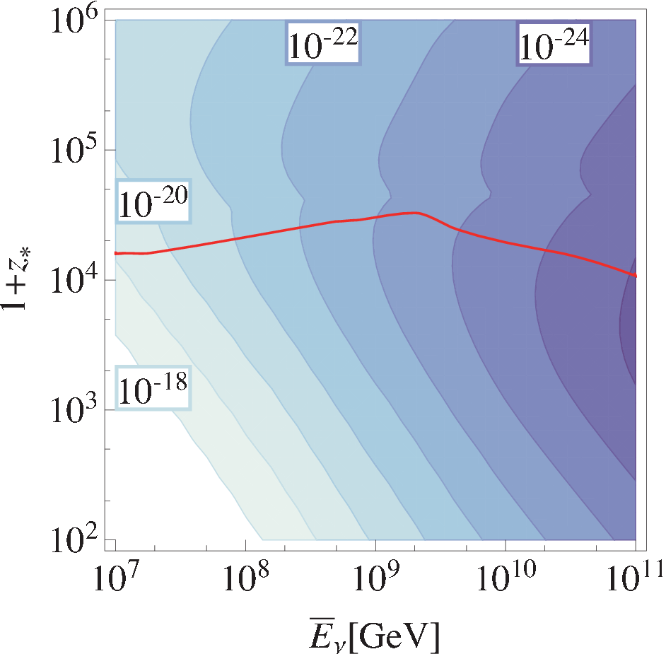
In Fig. 6, we show the lower limit on $Y_{X}$ for the $5\sigma$ detection with the expected PIXIE sensitivity. The shape of the contours reflects the dependences of $y$ and $\mu$ on $(\bar{E}_{\nu},z_{*})$ shown in Figs. 4 and 4. There are kink-like structures at $1+z_{*}\sim 5\times 10^{4}$. This is due to the fact that the injected energy is equally distributed into $y$ and $\mu$ in our approximation for such a redshift; the lowest value of $Y_{X}$ for the detection becomes slightly weaker. Then, above and below the kink, the value of $Y_{X}$ shown in Fig. 6 is obtained from the consideration of $\mu$- and $y$-type distortions, respectively.

Even with the expected sensitivity of the PIXIE experiment, the current bound on the neutrino flux provides better sensitivity to the present scenario if $1+z_{*}\stackrel{{\scriptstyle<}}{{{}_{\sim}}}2\times 10^{4}$. In Fig. 6, the boundary of such a region is indicated by the red line; in the region below the red line, the values of $Y_{X}$ shown in the figure are already excluded by the current bounds on the neutrino flux. In other words, for $1+z_{*}\stackrel{{\scriptstyle>}}{{{}_{\sim}}}2\times 10^{4}$ where the neutrino scattering is efficient, future observations of the CMB spectral distortions can test the parameter space which is not explored by the current data.

We also note here that the PRISM experiment may provide another accurate probe of the $y$- and $\mu$-parameters. In [16], it is claimed that the sensitivity of the PRISM experiment can be as good as $\Delta\rho_{\rm rad}/\rho_{\rm rad}\sim O(10^{-9})$, where $\Delta\rho_{\rm rad}$ is the total amount of the energy release from decaying particles, which may correspond to a better sensitivity than the PIXIE experiment. With detection sensitivities other than Eqs. (3.3) and (3.4), the value of $Y_{X}$ required for the detection of the signal can be obtained by rescaling the values shown in Fig. 6.

So far, we have assumed that $X$ dominantly decays into neutrinos. If electromagnetic particles are efficiently emitted by the decay of $X$, however, we should also consider constraints from these decay products. We briefly comment on such a case although it is beyond the scope of our study. When $1+z_{*}\stackrel{{\scriptstyle>}}{{{}_{\sim}}}2\times 10^{3}$, the electromagnetic particles produced by $X$ contribute to the $\mu$-type and $y$-type distortions or the dissociation processes of the light elements after causing the electromagnetic cascade discussed in Sec. 2.1. For $\tau(z;E)\stackrel{{\scriptstyle>}}{{{}_{\sim}}}1$, the neutrino scattering processes are so efficient that the neutrinos produced by $X$ also induce the electromagnetic cascade. As a result, if the same amount of neutrinos and electromagnetic particles are produced by $X$, the constraint on $Y_{X}$ due to the distortion of the CMB spectrum or the light-element abundances is expected to be more-or-less unchanged for such a parameter region. For $\tau(z;E)\stackrel{{\scriptstyle<}}{{{}_{\sim}}}1$, however, the constraint from electromagnetic particles due to the distortion of the CMB spectrum or the light-element abundances is stronger than that from neutrinos. When $1+z_{*}\stackrel{{\scriptstyle<}}{{{}_{\sim}}}2\times 10^{3}$, on the contrary, electromagnetic particles produced by $X$ may change the ionization history, which also gives the constraint on the injection of electromagnetic particles [22, 25, 27].

References

- [1] See, for example, A. Ibarra, D. Tran and C. Weniger, Int. J. Mod. Phys. A 28, no. 27, 1330040 (2013) [arXiv:1307.6434 [hep-ph]].
- [2] M. G. Aartsen et al. [IceCube Collaboration], Science 342, no. 6161, 1242856 (2013) [arXiv:1311.5238 [astro-ph.HE]].
- [3] M. G. Aartsen et al. [IceCube Collaboration], arXiv:1405.5303 [astro-ph.HE].
- [4] Y. Ema, R. Jinno and T. Moroi, Phys. Lett. B 733, 120 (2014) [arXiv:1312.3501 [hep-ph]].
- [5] B. Feldstein, A. Kusenko, S. Matsumoto and T. T. Yanagida, Phys. Rev. D 88, no. 1, 015004 (2013) [arXiv:1303.7320 [hep-ph]].
- [6] A. Esmaili and P. D. Serpico, JCAP 1311, 054 (2013) [arXiv:1308.1105 [hep-ph]].
- [7] Y. Bai, R. Lu and J. Salvado, arXiv:1311.5864 [hep-ph].
- [8] A. Bhattacharya, M. H. Reno and I. Sarcevic, JHEP 06, 110 (2014) [arXiv:1403.1862 [hep-ph]].
- [9] J. Zavala, arXiv:1404.2932 [astro-ph.HE].
- [10] C. -H. Chen and T. Nomura, arXiv:1404.2996 [hep-ph].
- [11] T. Higaki, R. Kitano and R. Sato, arXiv:1405.0013 [hep-ph].
- [12] L. A. Anchordoqui, V. Barger, I. Cholis, H. Goldberg, D. Hooper, A. Kusenko, J. G. Learned and D. Marfatia et al., Journal of High Energy Astrophysics 1-2, 1 (2014) [arXiv:1312.6587 [astro-ph.HE]].
- [13] D. J. Fixsen, E. S. Cheng, D. A. Cottingham, R. E. Eplee, R. B. Isaacman, J. C. Mather, S. S. Meyer and P. D. Noerdlinger et al., Astrophys. J. 420, 445 (1994).
- [14] D. J. Fixsen, E. S. Cheng, J. M. Gales, J. C. Mather, R. A. Shafer and E. L. Wright, Astrophys. J. 473, 576 (1996) [astro-ph/9605054].
- [15] A. Kogut, D. J. Fixsen, D. T. Chuss, J. Dotson, E. Dwek, M. Halpern, G. F. Hinshaw and S. M. Meyer et al., JCAP 1107, 025 (2011) [arXiv:1105.2044 [astro-ph.CO]].
- [16] P. André et al. [PRISM Collaboration], JCAP 1402 (2014) 006 [arXiv:1310.1554 [astro-ph.CO]].
- [17] M. C. Gonzalez-Garcia, M. Maltoni, J. Salvado and T. Schwetz, JHEP 1212, 123 (2012) [arXiv:1209.3023 [hep-ph]].
- [18] T. Sjostrand, S. Mrenna and P. Z. Skands, JHEP 0605, 026 (2006) [hep-ph/0603175].
- [19] T. Sjostrand, S. Mrenna and P. Z. Skands, Comput. Phys. Commun. 178, 852 (2008) [arXiv:0710.3820 [hep-ph]].
- [20] See, for example, V. b. Berestetsky, E. m. Lifshitz and L. p. Pitaevsky, “Quantum Electrodynamics,” Oxford, Uk (1982).
- [21] W. Hu and J. Silk, Phys. Rev. Lett. 70, 2661 (1993).
- [22] X. -L. Chen and M. Kamionkowski, Phys. Rev. D 70, 043502 (2004) [astro-ph/0310473].
- [23] S. R. Furlanetto, S. P. Oh and E. Pierpaoli, Phys. Rev. D 74, 103502 (2006) [astro-ph/0608385].
- [24] M. Valdes, A. Ferrara, M. Mapelli and E. Ripamonti, Mon. Not. Roy. Astron. Soc. 377, 245 (2007) [astro-ph/0701301].
- [25] L. Zhang, X. Chen, M. Kamionkowski, Z. -g. Si and Z. Zheng, Phys. Rev. D 76, 061301 (2007) [arXiv:0704.2444 [astro-ph]].
- [26] J. Chluba and R. A. Sunyaev, Mon. Not. Roy. Astron. Soc. 419, 1294 (2012) [arXiv:1109.6552 [astro-ph.CO]].
- [27] T. R. Slatyer, Phys. Rev. D 87, no. 12, 123513 (2013) [arXiv:1211.0283 [astro-ph.CO]].
- [28] R. Khatri and R. A. Sunyaev, JCAP 1209, 016 (2012) [arXiv:1207.6654 [astro-ph.CO]].
- [29] J. Chluba, Mon. Not. Roy. Astron. Soc. 434, 352 (2013) [arXiv:1304.6120 [astro-ph.CO]].
- [30] J. Chluba, arXiv:1304.6121 [astro-ph.CO].
- [31] J. Chluba and D. Jeong, arXiv:1306.5751 [astro-ph.CO].
- [32] Y. B. Zeldovich and R. A. Sunyaev, Astrophys. Space Sci. 4, 301 (1969).
- [33] R. A. Sunyaev and Y. B. Zeldovich, Astrophys. Space Sci. 7, 20 (1970).
- [34] L. Danese and G. de Zotti, Astron. Astrophys. 107, 39 (1982).
- [35] C. Burigana, G. de Zotti and L. Danese, Astrophys. J. 379, 1 (1991).
- [36] W. Hu and J. Silk, Phys. Rev. D 48, 485 (1993).
- [37] C. Burigana, G. de Zotti and L. Danese, Astron. Astrophys. 303, 323 (1995).
- [38] J. Chluba, R. Khatri and R. A. Sunyaev, Mon. Not. Roy. Astron. Soc. 425, 1129 (2012) [arXiv:1202.0057 [astro-ph.CO]].
- [39] T. R. Slatyer, N. Padmanabhan and D. P. Finkbeiner, Phys. Rev. D 80, 043526 (2009) [arXiv:0906.1197 [astro-ph.CO]].
- [40] M. Kawasaki, K. Kohri and T. Moroi, Phys. Lett. B 625, 7 (2005) [astro-ph/0402490].
- [41] M. Kawasaki, K. Kohri and T. Moroi, Phys. Rev. D 71, 083502 (2005) [astro-ph/0408426].
- [42] M. Kawasaki and T. Moroi, Phys. Lett. B 346, 27 (1995) [hep-ph/9408321].
- [43] T. Kanzaki, M. Kawasaki, K. Kohri and T. Moroi, Phys. Rev. D 76, 105017 (2007) [arXiv:0705.1200 [hep-ph]].
- [44] M. Honda, T. Kajita, K. Kasahara, S. Midorikawa and T. Sanuki, Phys. Rev. D 75, 043006 (2007) [astro-ph/0611418].
- [45] R. Abbasi et al. [IceCube Collaboration], Phys. Rev. D 84, 082001 (2011) [arXiv:1104.5187 [astro-ph.HE]].
- [46] M. G. Aartsen et al. [IceCube Collaboration], Phys. Rev. D 88, 112008 (2013) [arXiv:1310.5477 [astro-ph.HE]].
- [47] C. Y. Chen, P. S. Bhupal Dev and A. Soni, Phys. Rev. D 89, no. 3, 033012 (2014) [arXiv:1309.1764 [hep-ph]].
- [48] R. D. Peccei and H. R. Quinn, Phys. Rev. Lett. 38, 1440 (1977).
- [49] R. D. Peccei and H. R. Quinn, Phys. Rev. D 16, 1791 (1977).
- [50] M. Dine and A. E. Nelson, Phys. Rev. D 48, 1277 (1993) [hep-ph/9303230].
- [51] M. Dine, A. E. Nelson and Y. Shirman, Phys. Rev. D 51, 1362 (1995) [hep-ph/9408384].
- [52] M. Dine, A. E. Nelson, Y. Nir and Y. Shirman, Phys. Rev. D 53, 2658 (1996) [hep-ph/9507378].