Building Water Models, A Different Approach
Abstract
Simplified, classical models of water are an integral part of atomistic molecular simulations, especially in biology and chemistry where hydration effects are critical. Yet, despite several decades of effort, these models are still far from perfect. Presented here is an alternative approach to constructing point charge water models – currently, the most commonly used type. In contrast to the conventional approach, we do not impose any geometry constraints on the model other than symmetry. Instead, we optimize the distribution of point charges to best describe the “electrostatics” of the water molecule, which is key to many unusual properties of liquid water. The search for the optimal charge distribution is performed in 2D parameter space of key lowest multipole moments of the model, to find best fit to a small set of bulk water properties at room temperature. A virtually exhaustive search is enabled via analytical equations that relate the charge distribution to the multipole moments. The resulting “optimal” 3-charge, 4-point rigid water model (OPC) reproduces a comprehensive set of bulk water properties significantly more accurately than commonly used rigid models: average error relative to experiment is 0.76%. Close agreement with experiment holds over a wide range of temperatures, well outside the ambient conditions at which the fit to experiment was performed. The improvements in the proposed water model extend beyond bulk properties: compared to the common rigid models, predicted hydration free energies of small molecules in OPC water are uniformly closer to experiment, root-mean-square error kcal/mol.
keywords
water models, electrostatics, liquid structure simulations, optimal point charge approximation1 Introduction
Water is the most extensively studied molecule Kale and Herzfeld (2012); Tu and Laaksonen (2000); Dill et al. (2005), yet our understanding of how this deceptively simple compound of just three atoms gives rise to the many extraordinary properties of its liquid phase Finney (2001); Finney (2004); Ball (1999) is far from complete Stillinger (1980). The complexity of the water properties combined with multiple possible levels of approximations (e.g. quantum vs. classical, flexible vs. rigid) has led to the proposal of literally hundreds of theoretical and computational models for water Guillot (2002). Among these, the most simple and computationally efficient, rigid non-polarizable models that represent water as a set of point charges at fixed positions relative to the oxygen nucleus stand out as the class used in the vast majority of biomolecular studies today. Commonly used rigid models (e.g. TIP3P Jorgensen et al. (1983) and SPC/E Berendsen et al. (1987) 3-point models, TIP4P/Ew Horn et al. (2004) 4-point model, and the TIP5P Mahoney and Jorgensen (2000) 5-point model) have achieved a reasonable compromise between accuracy and speed, but are by no means perfect Guillot (2002); Mark and Nilsson (2001). In particular, none of these models faithfully reproduce all the key properties of bulk water simultaneously. The search for more accurate yet computationally facile water models is still very active Wang et al. (2014); Fuentes-Azcatl and Alejandre (2014); Wang et al. (2013); Fennell et al. (2012).

Many unique properties of liquid water are due to the ability of the water molecules to establish a hydrogen-bonded structure, through the attraction between the electropositive hydrogen atoms and the electronegative oxygen atoms Marechal (2007). Therefore, a key challenge in developing classical water models is to find an accurate yet simplified description of the charge distribution of the water molecule that can adequately account for the hydrogen bonding in the liquid phase. Procedures employed to develop commonly used rigid water models generally impose constraints on the geometry (OH bond length and HOH angle) based on experimental observations, most commonly by fixing the positive point charges at the hydrogen nuclei positions. The atomic partial charges and the Lennard-Jones potential parameters are then optimized to reproduce selected bulk properties of water Guillot (2002). This approach may not necessarily accurately reproduce the electrostatic characteristics of the water molecule due to severe constraints on allowed variations in the charge distribution being optimized. The configuration of three point charges to best describe the charge distribution of the water molecule can be very different from what one may intuitively expect based on its well-known atomic structure. Consider, for example, the gas-phase quantum-mechanical (QM) charge distribution of a water molecule, Figure 1. The shown tight clustering of the point charges away from the nuclei reproduces the electrostatic potential around the QM charge distribution considerably more accurately than the more traditional distribution with point charges placed on or near the nuclei. For the optimal charge placement, Figure 1, the maximum error in electrostatic potential at the experimental oxygen-Na+ distance (2.23 Å ) from the origin, is almost 5.4 times smaller than that of the nucleus-centered alternative (1.4 kcal/mol vs. 7.56 kcal/mol).
Intrigued by the idea that optimal placement of the point charges in a water model can be very different from the “intuitive” placement on the nuclei, and encouraged by the significant improvement of the accuracy of electrostatics brought about by this strategy in gas-phase, we explore what the approach can offer for building classical water models in the liquid phase. In what follows, we describe the construction and testing of a 4-point, rigid “optimal” point charge (OPC) water model.
2 Approach
Most unique properties of liquid water are due to the complexity of the hydrogen bonding interactions, which are primarily described by the electrostatic interactions Morokuma (1977) within classical potential functions, including those used in common water models. While the electrostatic interactions are complemented by a Lennard-Jones (LJ) potential, the latter is generally represented by a single site centered on the oxygen – the corresponding interaction is isotropic and featureless, in contrast to hydrogen bonding which is directional. Therefore, an accurate representation of electrostatic interactions is paramount for accurately accounting for hydrogen bonding and the properties of liquid water. In a search for the best “electrostatics”, commonly used distance and angle constraints on the configuration of a model’s point charges are therefore of little relevance to classical rigid water models, yet these constraints impede the search for the “best” model geometry. This observation leads to one of the key features of our approach: any “intuitive” constraints on point charges or their geometry (other than the fundamental C2v symmetry of water molecule) are completely abandoned here in favor of finding an optimal electrostatic charge distribution that best approximates liquid properties of water. While ultimately it is the values of the point charges and their relative positions that we seek, (Figure 2), we argue that the conventional “charge–distances–angles” space Jorgensen et al. (1983); Horn et al. (2004); Mahoney and Jorgensen (2000); Berendsen et al. (1987) is not optimal to perform the search for the best electrostatics model. These coordinates affect the resulting electrostatic potential in a convoluted manner, it is unclear which ones are key. On the other hand, any complex charge distribution can be systematically described by its multipole moments, with lower moments expected to have a more profound effect on liquid water properties Stone (1997). Therefore our second key proposal is to search for the optimal model geometry and point charges in a subspace of water multipole moments, which we can systematically vary. Clearly, any reasonable water model needs to account for the large dipole moment of water molecule in order to reproduce dielectric properties of the liquid state Fennell et al. (2012); Niu et al. (2011). At short distances where hydrogen bonds between water molecules form (2.8Å), the relevance of higher electrostatic moments is also significant. For instance, the larger component of the water quadrupole has a strong effect on the liquid water structure seen in simulations Niu et al. (2011), and on the phase diagram Abascal and Vega (2007). The next order terms – octupole moments – while presumably less influential, also affect water structure e.g. around ions Te and Ichiye (2010). An intricate interplay between the dipole, quadrupole and octupole moments gives rise to the experimentally observed charge hydration asymmetry of aqueous solvation – strong dependence of hydration free energy on the sign of the solute charge Mukhopadhyay et al. (2012); Mukhopadhyay et al. (2014). Therefore, we seek a fixed-charge rigid model that optimally represents the three lowest order multipole moments of the water molecule. The exhaustive search for the optimum is enabled by the third key feature of our approach: a set of analytical equations that relates key multipole moments to the positions and values of the point charges of the water model.
The specifics.
To optimally reproduce the three lowest order multipole moments for the water molecule charge distribution, a minimum of three point charges are needed Anandakrishnan et al. (2013). The most general configuration for a three point charge model consistent with symmetry of the water molecule is shown in Figure 2: the point charges are placed in a V-shaped pattern in the Y-Z plane. We follow convention Jorgensen et al. (1983); Horn et al. (2004); Mahoney and Jorgensen (2000); Berendsen et al. (1987) and place the single Lennard-Jones (LJ) site on the oxygen atom. The four parameters (,, and ) that completely define the charge distribution, (Figure 2), are uniquely determined via analytical equations introduced in Methods, to best reproduce a targeted set of three lowest order multipole moments (dipole, quadrupole and octupole) Anandakrishnan et al. (2013) as detailed below. The ability to independently vary the moments of the charge distribution, provided by these analytical expressions, allows a full exploration in the relevant subspace of the moments. Generally, the importance of the multipole moments are inversely related to their order. The highest order multipole moment here is the octupole that has two independent components ( and ), which we fix to high quality quantum mechanical (QM) predictions, QM/230TIP5P Coutinho et al. (2003), Table 1. The linear component of the quadrupole is known to be relatively small for the water molecule and not expected to be very important Rick (2004), therefore, we also simply set it to the known QM value ( QM/230TIP5P Coutinho et al. (2003), Table 1 ). This leaves the two most important components, the dipole () and the square quadrupole (), as the two key search parameters we vary. We attempt to find the best fit to six key bulk properties by exhaustively searching in the 2D space of and , Figure 3, within the ranges that reflect known experimental uncertainties Gregory et al. (1997) and those of QM calculations Site et al. (1999); Silvestrelli and Parrinello (1999), Table 1. The six target bulk properties are: static dielectric constant , self diffusion coefficient , heat of vaporization , density and the position and height of the first peak in oxygen-oxygen pair distribution functions. These properties are calculated from molecular dynamics (MD) simulations, see Methods and the SI. For every trial value of and (and the fixed values of , and ), the charge distribution parameters (,, and ) are analytically determined (see Methods).
| Model | [D] | [DÅ] | [DÅ] | [DÅ2] | [DÅ2] |
|---|---|---|---|---|---|
| EXP (liquid) Gregory et al. (1997) | 2.53 | NA | NA | NA | NA |
| SPC/E | 2.35 | 0.00 | 2.04 | -1.57 | 1.96 |
| TIP3P | 2.35 | 0.23 | 1.72 | -1.21 | 1.68 |
| TIP4P/Ew | 2.32 | 0.21 | 2.16 | -1.53 | 2.11 |
| TIP5P | 2.29 | 0.13 | 1.56 | -1.01 | 0.59 |
| AIMD1 Silvestrelli and Parrinello (1999) | 2.95 | 0.18 | 3.27 | NA | NA |
| AIMD2 Site et al. (1999) | 2.43 | 0.10 | 2.72 | NA | NA |
| QM/4MM Niu et al. (2011) | 2.49 | 0.13 | 2.93 | -1.73 | 2.09 |
| QM/4TIP5P Niu et al. (2011) | 2.69 | 0.26 | 2.95 | -1.70 | 2.08 |
| QM/230TIP5P Coutinho et al. (2003) | 2.55 | 0.20 | 2.81 | -1.52 | 2.05 |
| OPC | 2.48 | 0.20 | 2.3 | -1.484 | 2.068 |


For every charge distribution calculated as above, the value of the 12-6 Lennard-Jones (LJ) potential, which is mainly responsible for the liquid structure Rick (2004), is selected so that the location of the first peak of the oxygen-oxygen radial distribution function (RDF) is in agreement with recent experiment Skinner et al. (2013) (see Methods). The value of is optimized so that the experimental value for density is achieved. The parameters and can be optimized nearly independently due to the weak coupling between them Rick (2004).
The result of the above search procedure is a “quality map” of all possible water models in the space: the proposed OPC model is the one with the highest quality score.
3 Results and discussion
3.1 The proposed optimal point charge model
As described above, we have performed an exhaustive search in the space for the best fit to six target bulk properties of liquid water at ambient conditions, Figure 3. The entire region of the space was mapped out using initially a relatively coarse grid spacing (0.1 D and 0.1 DÅ) in each direction shown in Figure 3. At this point, the quality of each test water model – corresponding to a point on the map – is characterized by a quality score function (see Methods) from a recent comprehensive review Vega and Abascal (2011) based on the same six key bulk properties used for the fitting.
Accordingly each model is assigned a quality score, using the score function explained in the Methods section, and is shown in Figure 3. As demonstrated in Figure 3, the highest quality region (the green area) occurs for (2.4 D 2.6 D) and (2.2 DÅ 2.4 DÅ). The region is relatively small and this is why an exhaustive, fine-grain search was required to identify the best model, which we refer to as the Optimal Point Charge (OPC) model (Figure 3).

From Figure 3, one can see three distinct regions in the space: the “common water models” region with relatively small dipole and square quadrupole moments, the “QM” region characterized by larger dipole and square quadrupole, and narrow, high quality (OPC) region with intermediate values of these two key moments. Compared to the other rigid models shown, OPC reproduces the multipole moments of water molecule in the liquid phase substantially better. In fact, the OPC dipole moment (2.48 D) is in best agreement with the values from QM calculations and experiment. OPC’s (2.3 DÅ) is larger than the corresponding values of the common models, and is closest to the QM predictions (Figure 3, Table 1). By construction, OPC’s small component of the quadrupole matches the reference QM value, and its octupole moments are the best approximations. The improved accuracy of the OPC moments is an immediate consequence of the focus on electrostatics and the unrestricted fine-grain search in the space, which we believe is the most relevant subspace of the water multipole moments at this level of approximation. This important improvement became possible through the abandoning of the conventional geometrical constraints, allowing the moments to be varied independently; the availability of analytical equations that connected the charge distributions with multipole moments played an important role too.
While the OPC moments are closest to the QM values, they (in particular ) still deviate from the QM predictions (Table 1, Figure 3). The low quality of the test models in which the moments were close to the QM values (squares, Figure 3) suggests that, within the 3-charge models explored here, an analytical fit of moments to QM predictions does not guarantee agreement with experimental liquid phase properties. This discrepancy can be due to a number of limitations and approximations inherent to classical, rigid, non-polarizable water models, see e.g. Refs. Vega and Abascal (2011); Guillot (2002); Wang et al. (2013). Based on our own results, we suggest that another important factor may be the small number of point charges used to represent the complex charge distribution of real water molecule. Namely, a three point charge model is fundamentally unable to exactly reproduce the reference dipole, quadrupole and octupole moments simultaneously Anandakrishnan et al. (2013), and essentially has no control over the accuracy of its moments beyond the octupole. The contribution of the higher order multipole moments to electrostatic potential can be significant at close distances, which are relevant to water-water and water-ion interactions in liquid phase. We conjecture that the relatively small and value found at the highest quality region (green zone, Figure 3) compared to QM predictions (squares, Figure 3), may be a compromise to keep the higher moments not too far from optimal, ensuring a reasonable net electrostatic potential.
| [Å] | [Å] | |||||
|---|---|---|---|---|---|---|
| EXP(gas) | NA | 0.9572 | NA | 104.52 | NA | NA |
| TIP3P | 0.417 | 0.9572 | NA | 104.52 | 582.0 | 595.0 |
| TIP4PEw | 0.5242 | 0.9572 | 0.125 | 104.52 | 656.1 | 653.5 |
| TIP5P | 0.241 | 0.9572 | NA | 104.52 | 544.5 | 590.3 |
| SPC/E | 0.4238 | 1.0 | NA | 109.47 | 629.4 | 625.5 |
| OPC | 0.6791 | 0.8724 | 0.1594 | 103.6 | 865.1 | 858.1 |
The OPC point charge positions and values and the LJ parameters are listed in Table 2. The distances for OPC are shorter (0.8724Å), and the angle (Figure 2) is slightly narrower () than the corresponding experimental values of bond and HOH angle for the water molecule in the gas phase (0.9572Å and ). The charge magnitudes of the OPC model are significantly larger than those of other common models (Table 2). Although the OPC charge distribution is not as tightly clustered as the configuration of the optimal charge model in the gas phase (Figure 1), the deviation of OPC geometry from that of other models and the water molecule in the gas phase is influential. In particular, the quality of water models is extremely sensitive to the values of electrostatic multipole moments (Figure 3), which by itself are very sensitive to the geometrical parameters (Eqs. 10-12, and SI).
3.2 Bulk properties
Since the geometry of the proposed rigid, non-polarizable OPC model optimized for the liquid phase, Figure 2, is very different from the expected optimum outside of the liquid phase, Figure 1, here we test OPC model in the liquid phase only. The quality of the model in reproducing experimental bulk water properties at ambient conditions, and a comparison with other most commonly used rigid models is presented in Table 3. For 11 key liquid properties (Table 3) against which water models are most often benchmarked Vega and Abascal (2011); Vega et al. (2009); Horn et al. (2004), our proposed model is within 1.8 of the corresponding experimental value, except for one property (thermal expansion coefficient) that deviates from experiment by about 5. The full oxygen-oxygen radial distribution function (RDF), , is presented in the SI. By design, the experimental position of first peak in RDF is accurately reproduced by OPC. The position and height of other peaks are also closely reproduced.
| Property | TIP4PEw Horn et al. (2004) | SPCE Vega and Abascal (2011); Wang et al. (2014) | TIP3P Vega and Abascal (2011); Mahoney and Jorgensen (2000) | TIP5P Vega and Abascal (2011); Mahoney and Jorgensen (2000) | OPC | EXP Vega and Abascal (2011); Vega et al. (2009); Skinner et al. (2013) |
|---|---|---|---|---|---|---|
| () | 2.32 | 2.352 | 2.348 | 2.29 | 2.48 | 2.5–3 |
| 0.995 | 0.994 | 0.980 | 0.979 | 0.9970.001 | 0.997 | |
| 63.90 | 68 | 94 | 92 | 78.40.6 | 78.4 | |
| 2.44 | 2.54 | 5.5 | 2.78 | 2.30.02 | 2.3 | |
| 10.58 | 10.43 | 10.26 | 10.46 | 10.570.004 | 10.52 | |
| [Å] | 2.755 | 2.75 | 2.77 | 2.75 | 2.80 | 2.80 |
| a | 0.52 | 0.42 | 0.43 | 0.13 | 0.51 | 0.51 |
| 19.2 | 20.7 | 18.74 | 29 | 18.00.05 | 18 | |
| 3.2 | 5.0 | 9.2 | 6.3 | 2.70.1 | 2.56 | |
| 48.1 | 46.1 | 57.4 | 41 | 45.51 | 45.3 | |
| 276 | 241 | 182 | 277 | 272 | 277 |
a Values are calculated in this work. The experimental value is a theoretical estimate Mukhopadhyay et al. (2012) based on experimental hydration energies of pair Schmid et al. (2000). See SI for details.

While commonly used models may be in good agreement with experiment for certain properties, Figure 4, they often produce large errors (sometimes amounting to over 250) in some other key properties. In contrast, OPC shows a uniformly good agreement across all the bulk properties considered here.
The ability of OPC to reproduce the temperature dependence of six key water properties is shown in Figure 5 (and SI). OPC is uniformly closest to experiment. It is noteworthy that the OPC model, which resulted from a search in the space of only two parameters ( and ) at only one thermodynamic condition (298.16 K and 1 bar) to fit a small subset of bulk properties, automatically reproduces a large number of bulk properties with a high accuracy across a wide range of temperatures. This is in contrast not only to commonly used, but also to some recent rigid Wang et al. (2014); Fuentes-Azcatl and Alejandre (2014) and polarizable models Wang et al. (2013) that generally employ massive and more specialized fits against multiple properties over a wide range of thermodynamic conditions. While noticeable advance in the accuracy of bulk properties is made by these latest models, the overall end result is not more accurate than OPC (see SI).


(a) Bulk density (b) Static dielectric constant

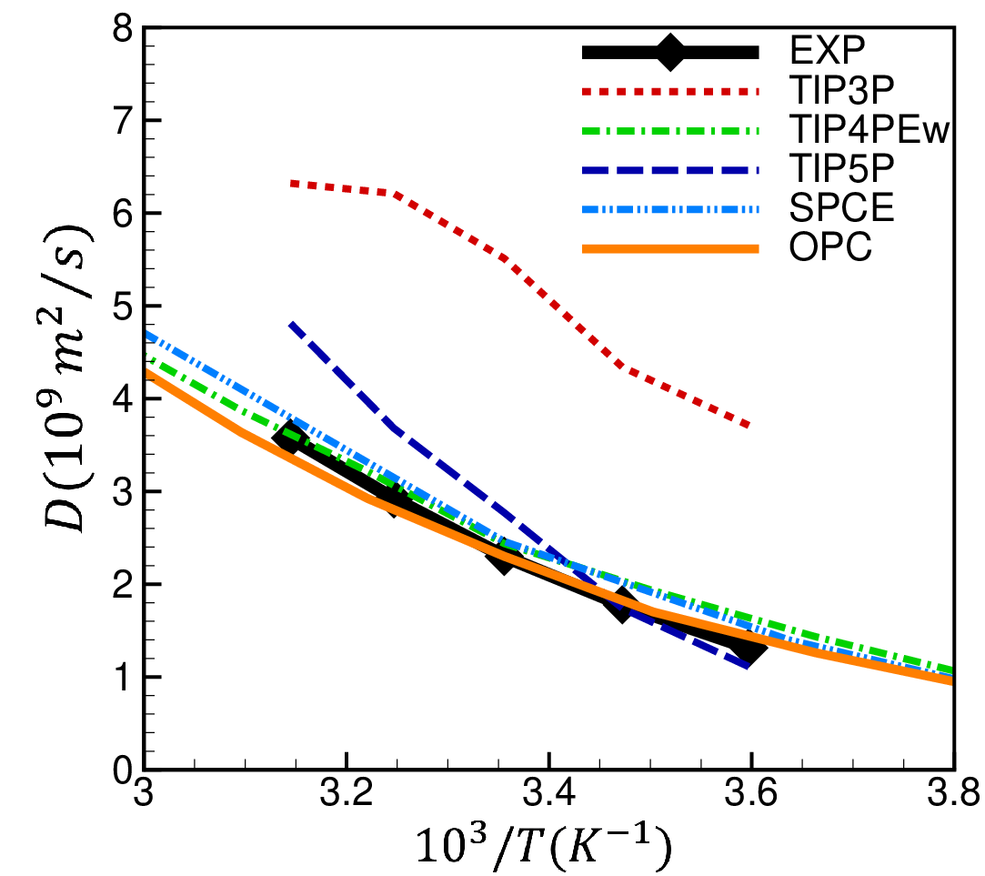
(c) Heat of vaporization (d) Self diffusion coefficient
3.3 Beyond bulk properties, OPC improvements matter for practical calculations
One of the main goals of developing better water models is improving the accuracy of simulated hydration effects in molecular systems. Here we show that the optimized charge distribution of OPC model does lead to a more accurate representation of solute-water interactions, whose accuracy is critical to the outcomes of atomistic simulations. One of the most sensitive measure of the balance of intermolecular and solute-water interaction is hydration free energy, which has been used to evaluate the accuracy of molecular mechanics force fields and water models alike Jorgensen and Tirado-Rives (2005). To evaluate OPC’s accuracy, we use a set of 20 molecules randomly selected to cover a wide range of experimental hydration energies from a large common test set of small molecules Mobley et al. (2009), see Methods. Compared to experiment, OPC predicts hydration free energy more accurately, on average (RMS error = 0.97 kcal/mol), as compared to 1.10 kcal/mol and 1.15 kcal/mol for TIP3P and TIP4PEw, respectively (Figure 6). The improvement is uniform across the range of solvation energies studied. The calculated average errors for OPC, TIP3P and TIP4PEw are 0.62, 0.78 and 0.87 kcal/mol, respectively, which shows that OPC is systematically more accurate than the other models tested. OPC is more accurate despite the fact that force fields have been historically parametrized against TIP3P. Somewhat paradoxically, TIP3P, which is certainly not the most accurate commonly used rigid model (see Figure 4), has nevertheless been generally known thus far to give the highest accuracy in hydration free energy calculations Mobley et al. (2009). The accuracy improvement by OPC is then noteworthy as it shows that an improvement in the “right direction” can indeed lead to improvement in free energy estimates. To the best of our knowledge, OPC is the only classical rigid model that predicts the solvation free energies of small molecules with the “chemical accuracy” (RMS error 1 kcal/mol).

4 Concluding Remarks
We have proposed a different approach to constructing classical water models. This approach recognizes that commonly used distance and angle constraints on the configuration of a model’s point charges are of little relevance to classical rigid water models; these artificial constraints complicate and impede the search for optimal charge distributions, key to reproducing unique features of liquid water. In our approach, such constraints are completely abandoned in favor of finding an optimal charge distribution (obeying only the fundamental C2v symmetry of water molecules) that best approximates properties of liquid water.
Next, we focus on the lowest multipole moments which directly control the electrostatics of the model. The hierarchical importance of these moments for water properties allowed us to reduce the search space to essentially just two key parameters: the dipole and the square quadrupole ( and ) moments; the less important moments were fixed to the QM-derived values. The low dimensionality of the parameter space, combined with a set of derived equations that connects the geometrical and charge values to its multipole moments, permitted a fine-grain exhaustive search virtually guaranteed to find an optimal solution within the accuracy class of the models considered here. The geometry of the resulting 4-point model (OPC) is different from commonly used ones, its location in the ( and ) is also distinctly different, which may explain why this optimum was not found previously via constrained optimization in higher dimensional space of geometrical parameters. The proposed model is significantly more accurate than other commonly used rigid models in reproducing bulk properties of liquid water. Although the optimization targeted a small subset of the properties at ambient conditions, the model reproduces a large number of bulk properties over a wide range of temperatures. The accuracy of predicted hydration free energies of small molecules has also improved, which is by no means an expected result: until now TIP3P model outperformed better quality rigid models in this respect. The consistently better accuracy offered by OPC demonstrates the benefits of fine-tuning electrostatic characteristics of classical water models.
We believe that the general approach presented here can be used to develop water models with different numbers of point charges, including presumably even more accurate -point () models, and also flexible and polarizable models. We expect that finding an -point charge optimum in the 2D parameter space (, ) is not going to be significantly more difficult than for the 4-point model presented here. The current 4-point OPC model is included in the solvent library of the Amber v14 molecular dynamics (MD) software package, and has been tested in GROMACS 4.6.5. The computational cost of running molecular dynamics simulations with it is the same as that for the popular TIP4P model.
5 Methods
5.1 Analytical solution for optimal point charges
Here we introduce the analytical equations that yield the positions and values of the three point charges that best reproduce the three lowest order multipole moments of the water molecule. The lowest three nonzero multipole moments of the water molecule are the dipole that is represented by one independent component (), the quadrupole defined by two independent components (, ), and the octupole defined by two independent components () Stone (1997). In the coordinate system shown in Figure 2, these moments are related to the Cartesian components of the traceless multipole moments of water molecule as , , , , and (see SI) Stone (1997); Rick (2004); Niu et al. (2011).
The optimal point charges are calculated so that these moments are sequentially reproduced, starting with the lowest order moments Anandakrishnan et al. (2013). The dipole and the quadrupole moments are reproduced exactly by requiring
| (1) | |||||
| (2) | |||||
| (3) |
where and are the independent unknown parameters that characterize the three point charge model (see Figure 2). The above set of equations is solved to find three geometrical parameters of the water model ( and )
| (4) | |||||
| (5) |
This leaves only one unknown parameter, the charge value q, which we calculate by using two additional equations that relate the charge distribution parameters to the octupole moment components so that the octupole moment is optimally reproduced Anandakrishnan et al. (2013) (see SI).
5.2 Calculation of bulk properties
The calculations of thermodynamic and dynamical bulk properties were done based on standard equations in the literature (see SI for details). Unless specified otherwise, we use the following Molecular Dynamics (MD) simulations protocol. Simulations in the NPT ensemble (1 bar, 298.16 K) were carried out using the Amber suite of programs. A cubic box with edge length of 30Å was filled with 804 water molecules. Periodic boundary condition was implemented in all directions. Long-range electrostatic interactions, calculated via the particle mesh Ewald (PME) summation, and the van der Waals interactions were cut off at distance 8Å . Dynamics were conducted with a 2 fs time step and all intra-molecular geometries were constrained with SHAKE. The NPT simulations were performed using Langevin thermostat with a coupling constant 2.0 and a Berendsen barostat with coupling constant of 1.0 for equilibration and 3.0 for production. The duration of production runs vary between 1 ns to 65 ns, depending on the properties (see SI).
5.3 Solvation free energy calculations
To avoid uncertainties due to conformational variability, the 20 test molecule were randomly selected from a subset of 248 highly rigid molecules Mukhopadhyay et al. (2014). Explicit solvent free energies calculations (via Thermodynamic Integration) were performed in GROMACS 4.6.5 Pronk et al. (2013) using the GAFF Wang et al. (2004) small molecule parameters, see SI for further details.
5.4 Scoring function
The predictive power of models against experimental data was validated using a scoring system developed by Vega et. al. Vega and Abascal (2011). For a calculated property and a corresponding experimental value of , the assigned score is obtained as Vega and Abascal (2011)
| (6) |
where the tolerance (tol) is assigned to 0.5% for density, position of the first peak in the RDF and heat of vaporization, 5% for height of the first peak in the RDF, and 2.5% for the remaining properties. The quality score assigned to each test model is equal to the average of the scores in bulk properties considered.
6 Supplementary Materials
6.1 Analytical solution for optimal point charges
Here we present the analytical equations to find three point charges that optimally reproduce the dipole, the quadrupole and the octupole moments of the water molecule. In the coordinate system shown in Fig. 2 (main text), the elements of the traceless dipole , quadrupole and octupole tensors Anandakrishnan et al. (2013) are
| (7) |
| (8) |
| (9) |
where and , and and are the dipole, the linear component of the quadrupole, the square component of the quadrupole, the linear component of the octupole, the square component of the octupole, respectively Stone (1997); Niu et al. (2011). The other elements of the octupole tensor () can be found by symmetry. The optimal charge values and positions are calculated so that these three moments are sequentially reproduced, starting with the lowest order moments Anandakrishnan et al. (2013). The first two lowest order moments of the water molecule, the dipole and the quadrupole, are fully reproduced by requiring
| (10) | |||||
| (11) | |||||
| (12) |
where and are independent unknown parameters that characterize the three point charge model (see Fig. 2). The above three equations are solved to find three geometrical parameters ( and y), as follows
| (13) | |||
| (14) |
For a given value of q, the values of and found as above exactly reproduce the dipole () and the quadrupole ( and ) moments of interest. The only remaining unknown parameter, q, is found to optimally reproduce the next order moment, the octupole, which is described by two independent parameters ( and ). The components of the octupole moment are related to the charge distribution parameters through
| (15) | |||||
| (16) |
The octupole tensor (Eq. 9) can be optimally approximated if the largest absolute principal value of the octupole tensor (i.e. for the water molecule) is reproduced Anandakrishnan et al. (2013). Therefore, we set () from Eqs. 15 and 16 and solve for q as
| (17) | |||||
The above solution is valid only when . For , the point charge positions converge to a singular point and the charge values go to infinity. The corresponding region in map (Fig. 3) leading to this condition is displayed in deepest red (zero score).
6.2 Solvation free energy calculations
Standard thermodynamics integration (TI) protocol was adopted from Ref. Mobley et al. (2009). The Merck-Frosst implementation of AM1-BCC Jakalian et al. (2000); Jakalian et al. (2002) was used to assign the partial charges. The topology and coordinates for the molecules were obtained from Ref. Mobley et al. (2009). Molecules were solvated in triclinic box with at least 12 Å from the solute to the nearest box edge. After minimization and equilibration, we performed standard free energy perturbation calculations using 20 values. Real space electrostatic cutoff was 10 Å. All bonds were restrained using the LINCS algorithm. Production NPT simulations were performed for 5ns. Identical simulations were performed for TIP3P, TIP4PEw, and OPC.
6.3 Calculating the bulk properties
The calculation of bulk properties were done based on standard equations in the literature Horn et al. (2004); Wu et al. (2006); Abascal and Vega (2005); Fuentes-Azcatl and Alejandre (2014). Unless stated otherwise, values of OPC at ambient temperature (Table 3) are given as averages over six independent simulations of 65 ns each, except for those quantities that are derived from temperature dependent results. The temperature dependent results are calculated from one simulation of 65 ns for each temperature point, i.e. 12.5K intervals in a temperature range [248K, 373K]. Details of the calculations of studied quantities are described below.
6.3.1 Static dielectric constant
The static dielectric constant is determined through Horn et al. (2004); Abascal and Vega (2005); Fuentes-Azcatl and Alejandre (2014)
| (18) |
where , is the position of atom i, is the Boltzmann constant, is the absolute temperature and is the simulation box average volume.
6.3.2 Self diffusion coefficient
The self-diffusion coefficient is obtained using the Einstein relation Horn et al. (2004); Fuentes-Azcatl and Alejandre (2014); Wu et al. (2006)
| (19) |
The simulation protocol to compute the self-diffusion coefficient is similar to the protocol described in Ref. Horn et al. (2004); the well equilibrated NPT simulations were followed up with 80 successive intervals of NVE (20 ps) and NPT (5 ps) ensembles. The self diffusion was obtained by averaging values over all the NVE runs.
6.3.3 Heat of vaporization
The heat of vaporization is obtained following the method described in Ref. Horn et al. (2004), as
| (20) |
where is the potential energy of the liquid with molecules at a given external pressure and a temperature , and is the average volume of the simulation box. is the ideal gas constant. accounts for the energetic cost of the effective polarization energy, and can be approximated as
| (21) |
where is the dipole moment of the corresponding rigid model and and are the dipole moment and the mean polarizability of a water molecule in the gas phase gui (2001), respectively. The OPC’s dipole is close to experiment and larger than that of common rigid models which yields a relatively larger value of for OPC compared to common rigid models. The correction term C, which accounts for vibrational, nonideal gas, and pressure effect, for various temperatures is taken from Ref. Horn et al. (2004).
6.3.4 Isobaric heat capacity
The isobaric heat capacity is determined through numeric differentiation of simulated enthalpies over the range of temperatures of interest Horn et al. (2004); Wu et al. (2006)
| (22) |
where ( at ) is a quantum correction term accounting for the quantized character of the neglected intramolecular vibrations. The values of for different temperatures are taken from Ref. Horn et al. (2004). The numeric differentiation is calculated from simulations in the temperature range [248K, 373K] in 12.5K increments.
6.3.5 Thermal expansion coefficient
The thermal expansion coefficient can be approximated through numeric differentiation of simulated bulk-densities over a range of temperatures of interest Horn et al. (2004); Wu et al. (2006); Fuentes-Azcatl and Alejandre (2014)
| (23) |
The reported value at ambient conditions is calculated from a numeric differentiation of bulk-densities at =296K and =300K, averaged over 4 independent simulations.
6.3.6 Isothermal compressibility
The isothermal compressibility is calculated from volume fluctuations in NPT simulation using a Langevin thermostat with coupling constant 2.0 and a Monte Carlo barostat with coupling constant of 3.0 , via the following formula Horn et al. (2004); Abascal and Vega (2005); Fuentes-Azcatl and Alejandre (2014)
| (24) |
Simulations of 65ns and 15ns time length were performed to obtain the temperature dependent results for () and (), respectively.
6.3.7 Propensity for Charge Hydration Asymmetry
Propensity of a water model to cause Charge Hydration Asymmetry (CHA) for a similar size cation/anion pair () such as is defined in Ref. Mukhopadhyay et al. (2012) as
| (25) |
where the term on the right is an approximation of propensity for CHA for point charge water models Mukhopadhyay et al. (2012), is the ion-water distance, is the free energy of hydration, and and are the dipole and the nontraceless quadrupole moment of the model, respectively Stone (1997).
6.4 Additional bulk properties, comparison with most recent models
6.4.1 O-O radial distribution function
Each potential OPC model is parametrized to exactly reproduce the position of the first peak. The positions and the heights of the remaining peaks are very accurately reproduced with these parameters. The height of the first peak is however slightly high, which leads to an average O-O coordination number () larger than experiment. This may be because of the repulsion in the LJ potential that is known to create an over structured liquid Kiss and Baranyai (2013); Guillot (2002). It is argued that using a softer potential (e.g. a simple exponential in the form of ) can correct the height of the first peak Kiss and Baranyai (2013). We employ a 12-6 potential to achieve compatibility with standard biomolecular force fields. While TIP3P is the only model that accurately reproduces the height of the first peak, it lacks structure beyond the first coordination shell (Fig. 7).


6.4.2 Isobaric heat capacity, isothermal compressibility, recent models


References
- Kale and Herzfeld (2012) Kale, S.; Herzfeld, J. J Chem Phys 2012, 136, 084109+.
- Tu and Laaksonen (2000) Tu, Y.; Laaksonen, A. Chem Phys Lett 2000, 329, 283–288.
- Dill et al. (2005) Dill, K. A.; Truskett, T. M.; Vlachy, V.; Hribar-Lee, B. Annu Rev Bioph Biom 2005, 34, 173–199.
- Finney (2001) Finney, J. L. J Mol Liq 2001, 90, 303 – 312.
- Finney (2004) Finney, J. L. Philosophical Transactions of the Royal Society of London. Series B: Biological Sciences 2004, 359, 1145–1165.
- Ball (1999) Ball, P. Life’s Matrix: A Biography of Water; Farrar, Straus, and Giroux, New York, 1999.
- Stillinger (1980) Stillinger, F. H. Science 1980, 209, pp. 451–457.
- Guillot (2002) Guillot, B. J Mol Liq 2002, 101, 219–260.
- Jorgensen et al. (1983) Jorgensen, W. L.; Chandrasekhar, J.; Madura, J. D.; Impey, R. W.; Klein, M. L. J Chem Phys 1983, 79, 926–935.
- Berendsen et al. (1987) Berendsen, H. J. C.; Grigera, J. R.; Straatsma, T. P. J Phys Chem 1987, 91, 6269–6271.
- Horn et al. (2004) Horn, H. W.; Swope, W. C.; Pitera, J. W.; Madura, J. D.; Dick, T. J.; Hura, G. L.; Head-Gordon, T. J Chem Phys 2004, 120, 9665–9678.
- Mahoney and Jorgensen (2000) Mahoney, M. W.; Jorgensen, W. L. J Chem Phys 2000, 112, 8910–8922.
- Mark and Nilsson (2001) Mark, P.; Nilsson, L. J Phys Chem A 2001, 105, 9954–9960.
- Wang et al. (2014) Wang, L. P.; Martinez, T. J.; Pande, V. S. J Phys Chem Lett 2014, 5, 1885–1891.
- Fuentes-Azcatl and Alejandre (2014) Fuentes-Azcatl, R.; Alejandre, J. J Phys Chem B 2014, 118, 1263–1272.
- Wang et al. (2013) Wang, L.-P.; Head-Gordon, T.; Ponder, J. W.; Ren, P.; Chodera, J. D.; Eastman, P. K.; Martinez, T. J.; Pande, V. S. J Phys Chem B 2013, 117, 9956–9972.
- Fennell et al. (2012) Fennell, C. J.; Li, L.; Dill, K. A. J Phys Chem B 2012, 116, 6936–6944.
- Anandakrishnan et al. (2013) Anandakrishnan, R.; Baker, C.; Izadi, S.; Onufriev, A. V. PLoS ONE 2013, 8, e67715.
- Marechal (2007) Marechal, Y. The Hydrogen Bond and the Water Molecule: The Physics and Chemistry of Water, Aqueous and Bio Media; Elsevier: Oxford, 2007.
- Morokuma (1977) Morokuma, K. Accounts Chem Res 1977, 10, 294–300.
- Stone (1997) Stone, A. The Theory of Intermolecular Forces; International Series of Monographs on Chemistry; Clarendon Press, 1997.
- Niu et al. (2011) Niu, S.; Tan, M. L.; Ichiye, T. J Chem Phys 2011, 134, 134501+.
- Abascal and Vega (2007) Abascal, J. L. F.; Vega, C. J Phys Chem C 2007, 111, 15811–15822.
- Te and Ichiye (2010) Te, J. A.; Ichiye, T. Chem Phys Lett 2010, 499, 219–225.
- Mukhopadhyay et al. (2012) Mukhopadhyay, A.; Fenley, A. T.; Tolokh, I. S.; Onufriev, A. V. J Phys Chem B 2012, 116, 9776–9783.
- Mukhopadhyay et al. (2014) Mukhopadhyay, A.; Aguilar, B. H.; Tolokh, I. S.; Onufriev, A. V. J Chem Theor Comp 2014, 10, 1788–1794.
- Coutinho et al. (2003) Coutinho, K.; Guedes, R.; Cabral, B. C.; Canuto, S. Chem Phys Lett 2003, 369, 345 – 353.
- Rick (2004) Rick, S. W. J Chem Phys 2004, 120, 6085–6093.
- Gregory et al. (1997) Gregory, J. K.; Clary, D. C.; Liu, K.; Brown, M. G.; Saykally, R. J. Science 1997, 275, 814–817.
- Site et al. (1999) Site, L. D.; Alavi, A.; Lynden-Bell, R. M. Mol Phys 1999, 96, 1683–1693.
- Silvestrelli and Parrinello (1999) Silvestrelli, P. L.; Parrinello, M. J Chem Phys 1999, 111, 3572–3580.
- Skinner et al. (2013) Skinner, L. B.; Huang, C.; Schlesinger, D.; Pettersson, L. G. M.; Nilsson, A.; Benmore, C. J. J Chem Phys 2013, 138, 074506.
- Vega and Abascal (2011) Vega, C.; Abascal, J. L. F. Phys Chem Chem Phys 2011, 13, 19663–19688.
- Vega et al. (2009) Vega, C.; Abascal, J. L. F.; Conde, M. M.; Aragones, J. L. Faraday Discuss. 2009, 141, 251–276.
- Mobley et al. (2008) Mobley, D. L.; Barber, A. E.; Fennell, C. J.; Dill, K. A. J Phys Chem B 2008, 112, 2405–2414.
- Rajamani et al. (2004) Rajamani, S.; Ghosh, T.; Garde, S. J Chem Phys 2004, 120, 4457–4466.
- Schmid et al. (2000) Schmid, R.; Miah, A. M.; Sapunov, V. N. Phys Chem Chem Phys 2000, 2, 97–102.
- Jorgensen and Jenson (1998) Jorgensen, W. L.; Jenson, C. J Comp Chem 1998, 19, 1179–1186.
- English * (2005) English *, N. J. Molecular Physics 2005, 103, 1945–1960.
- Jorgensen and Tirado-Rives (2005) Jorgensen, W. L.; Tirado-Rives, J. Proc Natl Acad Sci USA 2005, 102, 6665–6670.
- Mobley et al. (2009) Mobley, D. L.; Bayly, C. I.; Cooper, M. D.; Shirts, M. R.; Dill, K. A. J Chem Theor Comp 2009, 5, 350–358.
- Pronk et al. (2013) Pronk, S.; Páll, S.; Schulz, R.; Larsson, P.; Bjelkmar, P.; Apostolov, R.; Shirts, M. R.; Smith, J. C.; Kasson, P. M.; van der Spoel, D.; Hess, B.; Lindahl, E. Bioinformatics 2013, 29, 845–854.
- Wang et al. (2004) Wang, J.; Wolf, R. M.; Caldwell, J. W.; Kollman, P. A.; Case, D. A. J Comp Chem 2004, 25, 1157–1174.
- Jakalian et al. (2000) Jakalian, A.; Bush, B. L.; Jack, D. B.; Bayly, C. I. J Comp Chem 2000, 21, 132–146.
- Jakalian et al. (2002) Jakalian, A.; Jack, D. B.; Bayly, C. I. J Comp Chem 2002, 23, 1623–1641.
- Wu et al. (2006) Wu, Y.; Tepper, H. L.; Voth, G. A. J Chem Phys 2006, 124, 024503+.
- Abascal and Vega (2005) Abascal, J. L. F.; Vega, C. J Chem Phys 2005, 123, 234505+.
- gui (2001) Guideline on the Use of Fundamental Physical Constants and Basic Constants of Water; The International Association for the Properties of Water and Steam: Gaithersburg, Maryland, 2001.
- Kiss and Baranyai (2013) Kiss, P. T.; Baranyai, A. J Chem Phys 2013, 138, 204507+.