Synchronization under matrix-weighted Laplacian

S. Emre Tuna Note: The author is with Department of Electrical and Electronics Engineering, Middle East Technical University, 06800 Ankara, Turkey. Email: tuna@eee.metu.edu.tr

Abstract

Synchronization in a group of linear time-invariant systems is studied where the coupling between each pair of systems is characterized by a different output matrix. Simple methods are proposed to generate a (separate) linear coupling gain for each pair of systems, which ensures that all the solutions converge to a common trajectory. Both continuous-time and discrete-time cases are considered.

1 Introduction

Synchronization (consensus) of linear systems with general dynamics (as opposed to first- or second-order integrators) has been thoroughly investigated in the last decade. Early results established the convergence of the solutions of coupled systems to a common trajectory via static linear feedback under the condition that the network topology is fixed [10, 11]. Later, time-varying topologies were allowed in [12]. As the limitations of the static feedback have gradually been overcome, more general results employing dynamic feedback emerged; see, for instance, [9, 5] for fixed and [8, 6] for time-varying topologies.

All of the above-mentioned works, in fact the majority of the studies on synchronization of dynamical systems, cover the simple case

\displaystyle{\dot{x}}_{i}=\sum_{j=1}^{q}a_{ij}(x_{j}-x_{i})\,,\qquad i=1,\,2,\,\ldots,\,q

(1)

(where $a_{ij}\in{\mathbb{R}}_{\geq 0}$ and $x_{i}\in{\mathbb{R}}^{n}$ ) as a corollary of their main result. An equivalent representation of these systems reads ${\dot{x}}=-[L_{1}\otimes I_{n}]x$ where $x=[x_{1}^{T}\ x_{2}^{T}\ \cdots\ x_{q}^{T}]^{T}$ and $L_{1}\in{\mathbb{R}}^{q\times q}$ is the (weighted) Laplacian matrix [7] whose spectral properties have proved extremely useful in the analysis and design of multi-agent systems.

A pleasant thing about (1) is that its geometric meaning is clear: “Each agent moves towards the weighted average of the states of its neighbors.” as stated in [3]. In fact, in the Euler discretization

\displaystyle x_{i}^{+}=x_{i}+\varepsilon\sum_{j=1}^{q}a_{ij}(x_{j}-x_{i})=\sum_{j=1}^{q}w_{ij}x_{j}

(2)

the righthand side becomes the weighted average for $\varepsilon>0$ small enough. There are many ways to define average and, qualitatively speaking, what any average attempts to achieve is to compute some sort of center of the points considered in the computation. Therefore an excusable and sometimes even useful choice for weighted arithmetic mean is obtained by replacing the scalar weights $w_{ij}$ in (2) by symmetric positive semidefinite matrices $P_{ij}=P_{ij}^{T}\geq 0$ satisfying $\sum_{j}P_{ij}=I_{n}$ . This suggests on (1) the modification

\displaystyle{\dot{x}}_{i}=\sum_{j=1}^{q}Q_{ij}(x_{j}-x_{i})

where $Q_{ij}\in{\mathbb{R}}^{n\times n}$ are symmetric positive semidefinite matrices replacing the scalar weights $a_{ij}$ . (We take $Q_{ii}=0$ .) Whence follows the dynamics ${\dot{x}}=-Lx$ where

\displaystyle L=\left[\begin{array}[]{cccc}\sum_{j}Q_{1j}&-Q_{12}&\cdots&-Q_{1q}\\ -Q_{21}&\sum_{j}Q_{2j}&\cdots&-Q_{2q}\\ \vdots&\vdots&\ddots&\vdots\\ -Q_{q1}&-Q_{q2}&\cdots&\sum_{j}Q_{qj}\end{array}\right]_{qn\times qn}

is the matrix-weighted Laplacian. In graph theoretical terms one can say that the graph (with $q$ vertices) associated to this $L$ is such that to each edge a nonzero positive semidefinite matrix $Q_{ij}$ is assigned. Note that for the standard Laplacian the associated graph’s edges are assigned weights $a_{ij}$ that are merely positive scalars.

This paper deals with linear time-invariant systems. We consider a synchronization problem where the matrix-weighted Laplacian naturally appears as a tool for both analysis and design. In particular, we study a group of systems whose uncoupled dynamics (described by the matrix $A$ ) are identical and the communication between each pair $(i,\,j)$ of systems has to be realized via a (possibly) different output matrix $C_{ij}$ . Our goal for this setup is to generate linear gains $G_{ij}$ to couple the pairs so that all the solutions in the group converge to a common trajectory. For $A$ neutrally stable, we achieve this goal under detectability (of the pairs $(C_{ij},\,A)$ for $C_{ij}\neq 0$ ) and symmetry ( $C_{ij}=C_{ji}$ ). We also touch the more general situation (where $A$ is allowed to yield unbounded solutions) and establish synchronization under some additional conditions concerning detectability and the strength of connectivity of the network topology. We cover both continuous- and discrete-time cases. Synchronization in an array where each pair of systems are connected through a different output matrix $C_{ij}$ giving rise to the matrix-weighted Laplacian is yet a relatively unexplored area. Among the few works investigating this generalized Laplacian matrix (in a system-theoretic setting) are [1, 2], where the authors analyze its spectral properties and study certain relevant applications in distributed control and estimation.

2 Motivation

In this section we provide two example arrays of coupled identical systems where the matrix-weighted Laplacian $L$ appears naturally, describing the interconnection of individual systems. The first array is mechanical, the latter electrical.

2.1 Coupled mass-spring systems

Refer to caption — Figure 1: Mass-spring system.

Consider the individual system in Fig. 1, where $p$ masses are connected by linear springs. Let $z^{[i]}\in{\mathbb{R}}$ be the displacement of the mass $m_{i}>0$ from the equilibrium. The spring constants are denoted by $k_{i}>0$ . Letting $z=[z^{[1]}\ z^{[2]}\ \cdots\ z^{[p]}]^{T}$ the model of this system reads $M{\ddot{z}}+Kz=0$ where $M={\rm diag}(m_{1},\,m_{2},\,\ldots,\,m_{p})$ and

\displaystyle K=\left[\begin{array}[]{ccccc}k_{1}+k_{2}&-k_{2}&0&\cdots&0\\ -k_{2}&k_{2}+k_{3}&-k_{3}&\cdots&0\\ 0&-k_{3}&k_{3}+k_{4}&\cdots&0\\ \vdots&\vdots&\vdots&\ddots&\vdots\\ 0&0&0&\cdots&k_{p}+k_{p+1}\end{array}\right]

Let now an array be formed by coupling $q$ replicas of this system in the arrangement shown in Fig. 2. If we let $z_{i}\in{\mathbb{R}}^{p}$ denote the displacement vector for the $i$ th system and $b_{ij}^{[k]}=b_{ji}^{[k]}\geq 0$ represent the viscous friction (damping) between the $k$ th masses of the systems $i$ and $j$ , we can write the dynamics of the coupled systems as $M{\ddot{z}}_{i}+Kz_{i}+\sum_{j=1}^{q}B_{ij}({\dot{z}}_{i}-{\dot{z}}_{j})=0$ where $B_{ij}={\rm diag}(b_{ij}^{[1]},\,b_{ij}^{[2]},\,\ldots,\,b_{ij}^{[p]})$ . Letting $x_{i}=[z_{i}^{T}\ {\dot{z}}_{i}^{T}]^{T}$ denote the state of the $i$ th system we at once obtain

\displaystyle{\dot{x}}_{i}=\left[\begin{array}[]{cc}0&I_{p}\\ -M^{-1}K&0\end{array}\right]x_{i}+\sum_{j=1}^{q}\left[\begin{array}[]{cc}0&0\\ 0&M^{-1}B_{ij}\end{array}\right](x_{j}-x_{i})

Under the coordinate change below

\displaystyle\xi_{i}:=\left[\begin{array}[]{cc}K^{1/2}&0\\ 0&M^{1/2}\end{array}\right]x_{i}

we can transform (2.1) into

\displaystyle{\dot{\xi}}_{i}=S\xi_{i}+\sum_{j=1}^{q}Q_{ij}(\xi_{j}-\xi_{i})

(15)

where

\displaystyle S:=\left[\begin{array}[]{cc}0&K^{1/2}M^{-1/2}\\ -M^{-1/2}K^{1/2}&0\end{array}\right]\quad\mbox{and}\quad Q_{ij}:=\left[\begin{array}[]{cc}0&0\\ 0&M^{-1/2}B_{ij}M^{-1/2}\end{array}\right]

Note that $S$ is skew-symmetric and $Q_{ji}=Q_{ij}=Q_{ij}^{T}\geq 0$ . Finally, stacking the individual states into a single vector $\xi=[\xi_{1}^{T}\ \xi_{2}^{T}\ \cdots\ \xi_{q}^{T}]^{T}$ the dynamics of the array take the form

\displaystyle{\dot{\xi}}=([I_{q}\otimes S]-L)\xi

where $L$ is as defined in (1).

2.2 Coupled LC oscillators

Consider the individual system in Fig. 3, where $p$ linear inductors ( $L_{i}>0$ ) are connected by linear capacitors ( $C_{i}>0$ ). The node voltages are denoted by $z^{[i]}\in{\mathbb{R}}$ . Letting $z=[z^{[1]}\ z^{[2]}\ \cdots\ z^{[p]}]^{T}$ the model of this system reads $C{\ddot{z}}+L^{-1}z=0$ where $L={\rm diag}(L_{1},\,L_{2},\,\ldots,\,L_{p})$ and

\displaystyle C=\left[\begin{array}[]{ccccc}C_{1}+C_{2}&-C_{2}&0&\cdots&0\\ -C_{2}&C_{2}+C_{3}&-C_{3}&\cdots&0\\ 0&-C_{3}&C_{3}+C_{4}&\cdots&0\\ \vdots&\vdots&\vdots&\ddots&\vdots\\ 0&0&0&\cdots&C_{p}+C_{p+1}\end{array}\right]

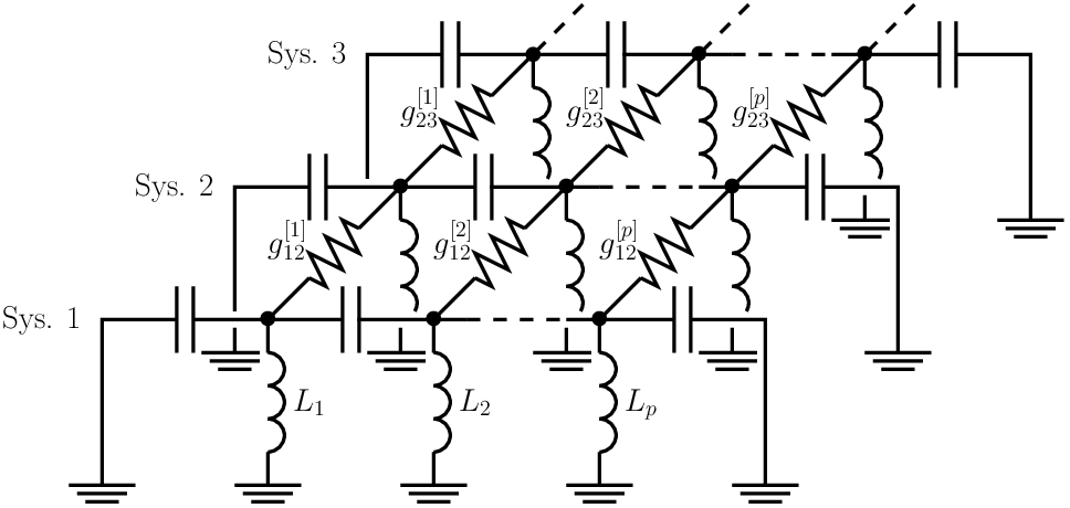
This time we form the array by coupling $q$ replicas of this system in the arrangement shown in Fig. 4. If we let $z_{i}\in{\mathbb{R}}^{p}$ denote the node voltage vector for the $i$ th system and $g_{ij}^{[k]}=g_{ji}^{[k]}\geq 0$ be the conductance of the resistor connecting the $k$ th nodes of the systems $i$ and $j$ , we can write the dynamics of the coupled systems as $C{\ddot{z}}_{i}+L^{-1}z_{i}+\sum_{j=1}^{q}G_{ij}({\dot{z}}_{i}-{\dot{z}}_{j})=0$ where $G_{ij}={\rm diag}(g_{ij}^{[1]},\,g_{ij}^{[2]},\,\ldots,\,g_{ij}^{[p]})$ . Letting $x_{i}=[z_{i}^{T}\ {\dot{z}}_{i}^{T}]^{T}$ denote the state of the $i$ th system we at once obtain

\displaystyle{\dot{x}}_{i}=\left[\begin{array}[]{cc}0&I_{p}\\ -C^{-1}L^{-1}&0\end{array}\right]x_{i}+\sum_{j=1}^{q}\left[\begin{array}[]{cc}0&0\\ 0&C^{-1}G_{ij}\end{array}\right](x_{j}-x_{i})

Under the coordinate change below

\displaystyle\xi_{i}:=\left[\begin{array}[]{cc}L^{-1/2}&0\\ 0&C^{1/2}\end{array}\right]x_{i}

we can transform (2.2) into

\displaystyle{\dot{\xi}}_{i}=S\xi_{i}+\sum_{j=1}^{q}Q_{ij}(\xi_{j}-\xi_{i})

(24)

where

\displaystyle S:=\left[\begin{array}[]{cc}0&L^{-1/2}C^{-1/2}\\ -C^{-1/2}L^{-1/2}&0\end{array}\right]\quad\mbox{and}\quad Q_{ij}:=\left[\begin{array}[]{cc}0&0\\ 0&C^{-1/2}G_{ij}C^{-1/2}\end{array}\right]

Note that $S$ is skew-symmetric and $Q_{ji}=Q_{ij}=Q_{ij}^{T}\geq 0$ . Finally, as was the case with the mechanical array, the dynamics of the electrical array reads ${\dot{\xi}}=([I_{q}\otimes S]-L)\xi$ where $L$ is the matrix-weighted Laplacian (1).

3 Problem definition

In this paper we consider a group of linear systems

{\dot{x}}_{i}&=Ax_{i}+u_{i}\,,\qquad i=1,\,2,\,\ldots,\,q\\ \mathcal{Y}_{i}=\{C_{i1}(x_{1}-x_{i}),\,C_{i2}(x_{2}-x_{i}),\,\ldots,\,C_{iq}(x_{q}-x_{i})\}

(26)

with $A\in{\mathbb{R}}^{n\times n}$ , where $x_{i}\in{\mathbb{R}}^{n}$ is the state and $u_{i}\in{\mathbb{R}}^{n}$ is the (control) input of the $i$ th system. The output set $\mathcal{Y}_{i}$ contains the relative measurements available to the $i$ th system, where $C_{ij}\in{\mathbb{R}}^{m_{ij}\times n}$ and $C_{ii}=0$ . Associated to the set $\{C_{ij}\}$ , we let the graph $\mathcal{G}=(\mathcal{V},\,\mathcal{E})$ represent the network topology, where $\mathcal{V}=\{v_{1},\,v_{2},\,\ldots,\,v_{q}\}$ is the set of vertices and a pair $(v_{j},\,v_{i})$ belongs to the set of edges $\mathcal{E}$ when $C_{ij}\neq 0$ .

The problem we study is the stabilization of the synchronization subspace of the systems (26). In particular, we search for a simple method for choosing the gains $G_{ij}\in{\mathbb{R}}^{n\times m_{ij}}$ such that under the controls

\displaystyle u_{i}=\sum_{j=1}^{q}G_{ij}C_{ij}(x_{j}-x_{i})

(27)

the systems (26) (asymptotically) synchronize. That is, the solutions satisfy $\|x_{i}(t)-x_{j}(t)\|\to 0$ as $t\to\infty$ for all indices $i,\,j$ and all initial conditions. We establish synchronization under two different sets of conditions. We first study the general case where the uncoupled dynamics ${\dot{z}}=Az$ are allowed to have unbounded solutions and provide certain sufficient conditions for synchronization. Later we will show that if $A$ is neutrally stable, which was the case with the mechanical and electrical arrays considered earlier, then synchronization can be achieved under much weaker assumptions.

4 Synchronization under CL-detectability

In this section we study synchronization under the assumption below.

Assumption 1

The following conditions hold on the systems (26).

1.

$C_{ij}=C_{ji}$ for all $i,\,j$ .
2.

$\mathcal{G}$ is connected.^*^* * Note that $\mathcal{G}$ becomes undirected under the first condition.
3.

There exists a symmetric positive definite matrix $P\in{\mathbb{R}}^{n\times n}$ such that

$\displaystyle A^{T}P+PA<C_{ij}^{T}C_{ij}\quad\mbox{for all}\quad C_{ij}\neq 0\,.$ (28)

Remark 1

Detectability of a pair $(C_{ij},\,A)$ is equivalent to the existence of a symmetric positive definite matrix $P_{ij}\in{\mathbb{R}}^{n\times n}$ satisfying $A^{T}P_{ij}+P_{ij}A<C_{ij}^{T}C_{ij}$ . (This is sometimes called the Lyapunov test for detectability [4].) The third condition of Assumption 1 therefore imposes a certain kind of uniformity on the detectability of the systems (26) by letting the detectability of all the individual pairs $(C_{ij},\,A)$ with $C_{ij}\neq 0$ be established by a common $P_{ij}=P$ . Therefore, referring to the condition (28), we will henceforth use the term CL-detectability, where C stands for common and L for Lyapunov.

Before we state our first theorem we introduce some notation related to the graph $\mathcal{G}=(\mathcal{V},\,\mathcal{E})$ associated to the systems (26). The degree $d_{i}$ of the vertex $v_{i}$ is the number of edges satisfying $(v_{j},\,v_{i})\in\mathcal{E}$ . We let $\Gamma=[\gamma_{ij}]\in{\mathbb{R}}^{q\times q}$ denote the unweighted, normalized Laplacian matrix defined as follows.

\displaystyle\gamma_{ij}=\left\{\begin{array}[]{rl}-1/q\,,&(v_{j},\,v_{i})\in\mathcal{E}\\ d_{i}/q\,,&j=i\\ 0\,,&\mbox{elsewhere}\end{array}\right.

When $\mathcal{G}$ is undirected and connected, $\Gamma$ is symmetric positive semidefinite with eigenvalues $0=\lambda_{1}<\lambda_{2}\leq\cdots\leq\lambda_{q}\leq 1$ . In that case we write $\lambda_{2}(\Gamma)$ to denote the smallest nonzero eigenvalue of $\Gamma$ . Let ${\mathbf{1}}\in{\mathbb{R}}^{q}$ be the vector of all ones and define $J:=I_{q}-q^{-1}{\mathbf{1}}{\mathbf{1}}^{T}$ . Note that $J$ is the unweighted, normalized Laplacian matrix of a complete graph and satisfies $\lambda_{2}(J)=1$ thanks to $J^{2}=J$ . Since $J$ and $\Gamma$ share the same eigenvectors (for $\mathcal{G}$ undirected and connected), one can readily establish the bounds

\displaystyle\Gamma\leq J\leq\lambda_{2}(\Gamma)^{-1}\Gamma\,.

(30)

Theorem 1

Consider the systems (26) under Assumption 1. Let $\alpha\geq(2q)^{-1}$ and $G_{ij}:=\alpha P^{-1}C_{ij}^{T}$ where $P$ satisfies (28). Then under the controls (27) the systems synchronize if

\displaystyle\varepsilon>(\lambda_{2}(\Gamma)^{-1}-1)\sigma

(31)

where $\displaystyle\varepsilon:=\min_{C_{ij}\neq 0}\,\lambda_{\rm min}(C_{ij}^{T}C_{ij}-A^{T}P-PA)$ and $\sigma:=\lambda_{\rm max}(A^{T}P+PA)$ .

Proof. Under the suggested controls, dynamics of the systems (26) become

\displaystyle{\dot{x}}_{i}=Ax_{i}+\sum_{j=1}^{q}{\alpha}P^{-1}C_{ij}^{T}C_{ij}(x_{j}-x_{i})\,,\qquad i=1,\,2,\,\ldots,\,q\,.

(32)

Letting $x=[x_{1}^{T}\ x_{2}^{T}\ \cdots\ x_{q}^{T}]^{T}$ and $Q_{ij}:=C_{ij}^{T}C_{ij}$ we can rewrite (32) as

\displaystyle{\dot{x}}=\left([I_{q}\otimes A]-\alpha[I_{q}\otimes P^{-1}]L\right)x=:\Psi x

(33)

where $L$ is the matrix-weighted Laplacian (1). Since $C_{ij}=C_{ji}$ the matrix $L$ is symmetric. It is also positive semidefinite because we can write

\displaystyle x^{T}Lx=\sum_{j>i}(x_{j}-x_{i})^{T}Q_{ij}(x_{j}-x_{i})=\sum_{j>i}\|C_{ij}(x_{j}-x_{i})\|^{2}\,.

Similarly, we can also write

$\displaystyle x^{T}\left([\Gamma\otimes(A^{T}P+PA)]-q^{-1}L\right)x$			(34)
	$\displaystyle=$	$\displaystyle q^{-1}\sum_{j>i}(x_{j}-x_{i})^{T}(A^{T}P+PA-Q_{ij})(x_{j}-x_{i})$
	$\displaystyle\leq$	$\displaystyle-q^{-1}\sum_{j>i}\varepsilon\\|x_{j}-x_{i}\\|^{2}$
	$\displaystyle=$	$\displaystyle-\varepsilon x^{T}[\Gamma\otimes I_{n}]x\,.$

By construction $L[{\mathbf{1}}\otimes I_{n}]=0$ . This allows us to write

$\displaystyle L[J\otimes I_{n}]$	$\displaystyle=$	$\displaystyle L[(I_{q}-q^{-1}{\mathbf{1}}{\mathbf{1}}^{T})\otimes I_{n}]$	(35)
	$\displaystyle=$	$\displaystyle L[I_{q}\otimes I_{n}]-q^{-1}L[{\mathbf{1}}\otimes I_{n}][{\mathbf{1}}^{T}\otimes I_{n}]$
	$\displaystyle=$	$\displaystyle L\,.$

By symmetry we also have $[J\otimes I_{n}]L=L$ . Define $V:{\mathbb{R}}^{qn}\to{\mathbb{R}}$ as $V(x):=x^{T}[J\otimes P]x$ . We will employ $V$ as a Lyapunov function for the synchronization subspace $\{x:x_{i}=x_{j}\ \mbox{for all}\ i,\,j\}\subset{\mathbb{R}}^{qn}$ . To this end, let us now study the time derivative of $V$ along the solutions of the array (33). Using (30), (34), and (35) we can write

$\displaystyle\Psi^{T}[J\otimes P]+[J\otimes P]\Psi$	$\displaystyle=$	$\displaystyle[J\otimes(A^{T}P+PA)]-\alpha(L[J\otimes I_{n}]+[J\otimes I_{n}]L)$
	$\displaystyle=$	$\displaystyle[J\otimes(A^{T}P+PA)]-2\alpha L$
	$\displaystyle\leq$	$\displaystyle[J\otimes(A^{T}P+PA)]-q^{-1}L$
	$\displaystyle=$	$\displaystyle[(J-\Gamma)\otimes(A^{T}P+PA)]$
		$\displaystyle\qquad+[\Gamma\otimes(A^{T}P+PA)]-q^{-1}L$
	$\displaystyle\leq$	$\displaystyle\sigma[(J-\Gamma)\otimes I_{n}]-\varepsilon[\Gamma\otimes I_{n}]$
	$\displaystyle\leq$	$\displaystyle(\lambda_{2}(\Gamma)^{-1}-1)\sigma[\Gamma\otimes I_{n}]-\varepsilon[\Gamma\otimes I_{n}]$
	$\displaystyle=$	$\displaystyle-(\varepsilon-(\lambda_{2}(\Gamma)^{-1}-1)\sigma)[\Gamma\otimes I_{n}]\,.$

Therefore we have established

\displaystyle\frac{d}{dt}V(x(t))\leq-\delta\,x(t)^{T}[\Gamma\otimes I_{n}]x(t)

(36)

where $\delta:=\varepsilon-(\lambda_{2}(\Gamma)^{-1}-1)\sigma$ . Now, since $[\Gamma\otimes I_{n}]$ is positive semidefinite, (36) implies the following. If (31) holds, i.e., $\delta>0$ , then the solutions converge to the set $\{x:x^{T}[\Gamma\otimes I_{n}]x=0\}$ , which is no other than the synchronization subspace. $\blacksquare$

When the graph $\mathcal{G}$ is complete, $\Gamma$ equals $J$ and $\lambda_{2}(\Gamma)=1$ . Then the condition (31) is satisfied automatically thanks to (28). Hence the result below.

Corollary 1

Consider the systems (26) under Assumption 1. Let $G_{ij}:=\alpha P^{-1}C_{ij}^{T}$ where $P$ satisfies (28) and $\alpha>0$ . Then under the controls (27) the systems synchronize for $\alpha$ large enough and $\mathcal{G}$ complete.

Note that any $\alpha\geq(2q)^{-1}$ is large enough by Theorem 1.

5 Synchronization under neutral stability

In the previous section we established synchronization of the systems (26) under the CL-detectability condition (28). In this section we show that this condition can be relaxed if the uncoupled dynamics harbor only bounded solutions. To this end, we make the assumption below.

Assumption 2

The following conditions hold on the systems (26).

1.

$C_{ij}=C_{ji}$ for all $i,\,j$ .
2.

$\mathcal{G}$ is connected.
3.

$A$ is neutrally stable.^†^† † In the continuous-time sense. That is, $A$ has no eigenvalue on the open right half-plane and for each eigenvalue on the imaginary axis the corresponding Jordan block is one-by-one.
4.

The pair $(C_{ij},\,A)$ is detectable^‡^‡ ‡ In the continuous-time sense. That is, no eigenvector of $A$ with eigenvalue on the closed right half-plane belongs to the null space of $C_{ij}$ . for all $C_{ij}\neq 0$ .

In Section 2 we observed that (after an appropriate coordinate change) both the mass-spring systems (15) and the LC oscillators (24) were represented by the highly-structured array dynamics ${\dot{\xi}}=([I_{q}\otimes S]-L)\xi$ , where $S$ was skew-symmetric and the matrix-weighted Laplacian $L$ was symmetric. This special righthand side, though it seems to pertain only to a narrow class of phenomena, in fact yields readily to generalization. For this reason we study it in the next lemma, which we will later extend to the main theorem of this section.

Lemma 1

Consider the group of systems

\displaystyle{\dot{\xi}}_{i}

\displaystyle=

\displaystyle S\xi_{i}+\sum_{j=1}^{q}H_{ij}^{T}H_{ij}(\xi_{j}-\xi_{i})\,,\qquad i=1,\,2,\,\ldots,\,q

(37)

where $S\in{\mathbb{R}}^{n\times n}$ and $H_{ij}\in{\mathbb{R}}^{m_{ij}\times n}$ with $H_{ii}=0$ . Let $\mathcal{H}$ be the graph associated to the set $\{H_{ij}\}$ . Assume that the following hold on the pair $(S,\,\{H_{ij}\})$ .

(C1)

$H_{ij}=H_{ji}$ for all $i,\,j$ .
(C2)

$\mathcal{H}$ is connected.
(C3)

$S$ is skew-symmetric.
(C4)

The pair $(H_{ij},\,S)$ is observable for all $H_{ij}\neq 0$ .

Then the systems synchronize. Moreover, the solutions $\xi_{i}(t)$ remain bounded.

Proof. Letting $\xi=[\xi_{1}^{T}\ \xi_{2}^{T}\ \cdots\ \xi_{q}^{T}]^{T}$ and $Q_{ij}:=H_{ij}^{T}H_{ij}$ we can rewrite (37) as

\displaystyle\dot{\xi}=([I_{q}\otimes S]-L)\xi

where $L$ is the matrix-weighted Laplacian (1). Since $H_{ij}=H_{ji}$ the matrix $L$ is symmetric. It is also positive semidefinite because we can write

\displaystyle x^{T}Lx=\sum_{j>i}(x_{j}-x_{i})^{T}Q_{ij}(x_{j}-x_{i})=\sum_{j>i}\|H_{ij}(x_{j}-x_{i})\|^{2}\,.

Thanks to the skew-symmetry of $S$ we have

\displaystyle([I_{q}\otimes S]-L)^{T}+([I_{q}\otimes S]-L)=[I_{q}\otimes(S+S^{T})]-(L+L^{T})=-2L\,.

Thus for the Lyapunov function $V(\xi)=2^{-1}\xi^{T}\xi=2^{-1}\|\xi\|^{2}$ we can write

\displaystyle\frac{d}{dt}V(\xi(t))

\displaystyle=

\displaystyle-\xi(t)^{T}L\xi(t)\,.

Since $L$ is positive semidefinite the solution $\xi(t)$ has to be bounded. (Hence the boundedness of the solutions $\xi_{i}(t)$ .) In particular, by LaSalle’s invariance principle, $\xi(t)$ should converge to the largest invariant set within the the intersection $\{\xi:\xi^{T}\xi\leq\|\xi(0)\|^{2}\}\cap\{\xi:\xi^{T}L\xi=0\}=:\mathcal{M}\subset{\mathbb{R}}^{qn}$ . To complete the proof therefore it should suffice to show that in this largest invariant set we have $\xi_{i}=\xi_{j}$ for all $i$ , $j$ .

Now let $\xi(t)$ be a solution that belongs identically to $\mathcal{M}$ . Suppose there exist indices $i_{1},\,i_{p}$ such that

\displaystyle\xi_{i_{1}}(t)\neq\xi_{i_{p}}(t)

(38)

for some $t\geq 0$ . Since $\xi(t)$ belongs identically to $\mathcal{M}$ we have $L\xi(t)\equiv 0$ . In other words

\displaystyle H_{ij}(\xi_{j}(t)-\xi_{i}(t))\equiv 0

(39)

for all $i,\,j$ . Then (37) is reduced to

\displaystyle{\dot{\xi}}_{i}=S\xi_{i}(t)

(40)

for all $i$ . By (39), (40), and the observability of the pairs $(H_{ij},\,S)$ (for $H_{ij}\neq 0$ ) we can therefore write $\xi_{i}(t)\equiv\xi_{j}(t)$ for all $H_{ij}\neq 0$ . Since the graph $\mathcal{H}$ is connected we can find indices $i_{2},\,i_{3},\,\ldots,\,i_{p-1}$ such that $H_{i_{\ell}i_{\ell+1}}\neq 0$ for $\ell=1,\,2,\,\ldots,\,p-1$ . Then we have $\xi_{i_{\ell}}(t)\equiv\xi_{i_{\ell+1}}(t)$ for $\ell=1,\,2,\,\ldots,\,p-1$ , which implies $\xi_{i_{1}}(t)\equiv\xi_{i_{p}}(t)$ . This contradicts (38). $\blacksquare$

A pleasant pair of byproducts of Lemma 1 are the following twin corollaries on the mechanical and electrical arrays studied in Section 2.

Corollary 2

Consider the coupled mass-spring systems (2.1). Let the graph associated to the set $\{B_{ij}\}$ be connected and the pairs $(M^{-1}B_{ij},\,M^{-1}K)$ be observable for all $B_{ij}\neq 0$ . Then the systems synchronize.

Corollary 3

Consider the coupled LC oscillators (2.2). Let the graph associated to the set $\{G_{ij}\}$ be connected and the pairs $(C^{-1}G_{ij},\,C^{-1}L^{-1})$ be observable for all $G_{ij}\neq 0$ . Then the oscillators synchronize.

In order to extend Lemma 1 to a general result we will need the following fact. (Most readers shall find the statement obvious. Still, for the sake of completeness, a demonstration is provided.)

Lemma 2

Let $A\in{\mathbb{R}}^{n\times n}$ be neutrally stable and the signal $w:{\mathbb{R}}_{\geq 0}\to{\mathbb{R}}^{n}$ satisfy $\|w(t)\|\leq ce^{-\alpha t}$ for some constants $c,\,\alpha>0$ . Then for each solution $x(t)$ of the system ${\dot{x}}(t)=Ax(t)+w(t)$ there exists $v\in{\mathbb{R}}^{n}$ such that $\|x(t)-e^{At}v\|\to 0$ as $t\to\infty$ .

Proof. If $A$ is stable (i.e., all its eigenvalues are in the open left half-plane) then we can choose $v=0$ . Otherwise let $T\in{\mathbb{R}}^{n\times n}$ be a transformation matrix such that

\displaystyle T^{-1}AT=\left[\begin{array}[]{cc}S&0\\ 0&F\end{array}\right]=:{\tilde{A}}

where $S\in{\mathbb{R}}^{n_{1}\times n_{1}}$ is skew-symmetric and $F\in{\mathbb{R}}^{n_{2}\times n_{2}}$ stable. Apply the coordinate change $z=[z_{1}^{T}\ z_{2}^{T}]^{T}=T^{-1}x$ with $z_{1}\in{\mathbb{R}}^{n_{1}}$ and $z_{2}\in{\mathbb{R}}^{n_{2}}$ and let $[{\tilde{w}}_{1}(t)^{T}\ {\tilde{w}}_{2}(t)^{T}]^{T}=T^{-1}w(t)$ with ${\tilde{w}}_{1}(t)\in{\mathbb{R}}^{n_{1}}$ and ${\tilde{w}}_{2}(t)\in{\mathbb{R}}^{n_{2}}$ . Then we can write

	$\displaystyle{\dot{z}}_{1}(t)$	$\displaystyle=$	$\displaystyle Sz_{1}(t)+{\tilde{w}}_{1}(t)$
	$\displaystyle{\dot{z}}_{2}(t)$	$\displaystyle=$	$\displaystyle Fz_{2}(t)+{\tilde{w}}_{2}(t)$

which yield

	$\displaystyle z_{1}(t)$	$\displaystyle=$	$\displaystyle e^{St}z_{1}(0)+\int_{0}^{t}e^{S(t-\tau)}{\tilde{w}}_{1}(\tau)d\tau$
	$\displaystyle z_{2}(t)$	$\displaystyle=$	$\displaystyle e^{Ft}z_{2}(0)+\int_{0}^{t}e^{F(t-\tau)}{\tilde{w}}_{2}(\tau)d\tau\,.$

Note that

\displaystyle\lim_{t\to\infty}z_{2}(t)=0

(42)

because $F$ is stable and ${\tilde{w}}_{2}(t)$ is exponentially decaying. Let

\displaystyle a:=\int_{0}^{\infty}e^{-S\tau}{\tilde{w}}_{1}(\tau)d\tau

which is well defined because $e^{St}$ is orthogonal (therefore bounded) and ${\tilde{w}}_{1}(t)$ is exponentially decaying. In particular, we have

\displaystyle\lim_{t\to\infty}\int_{t}^{\infty}e^{S(t-\tau)}{\tilde{w}}_{1}(\tau)d\tau=0\,.

(43)

Finally the below choice

\displaystyle v:=T\left[\begin{array}[]{c}z_{1}(0)+a\\ 0\end{array}\right]

should work. To see that we write

$\displaystyle\\|x(t)-e^{At}v\\|$	$\displaystyle=$	$\displaystyle\\|Tz(t)-Te^{{\tilde{A}}t}T^{-1}v\\|$
	$\displaystyle\leq$	$\displaystyle\\|T\\|\left(\\|z_{1}(t)-e^{St}(z_{1}(0)+a)\\|^{2}+\\|z_{2}(t)\\|^{2}\right)^{1/2}$
	$\displaystyle=$	$\displaystyle\\|T\\|\left(\left\\|\int_{t}^{\infty}e^{S(t-\tau)}{\tilde{w}}_{1}(\tau)d\tau\right\\|^{2}+\\|z_{2}(t)\\|^{2}\right)^{1/2}\,.$

The result follows by (42) and (43). $\blacksquare$

The below algorithm is where we construct the gains $G_{ij}$ that ensure synchronization under Assumption 2. The algorithm is followed by the main result of this section.

Algorithm 1

Given $A\in{\mathbb{R}}^{n\times n}$ that is neutrally stable and the set of matrices $\{C_{ij}\}$ with $C_{ij}\in{\mathbb{R}}^{m_{ij}\times n}$ , obtain the set $\{G_{ij}\}$ with $G_{ij}\in{\mathbb{R}}^{n\times m_{ij}}$ as follows. Let $n_{1}\leq n$ be the number of eigenvalues of $A$ on the imaginary axis and $n_{2}:=n-n_{1}$ . If $n_{1}=0$ let $G_{ij}:=0$ . Otherwise, first choose $U\in{\mathbb{R}}^{n\times n_{1}}$ and $W\in{\mathbb{R}}^{n\times n_{2}}$ satisfying

\displaystyle[U\ \ W]^{-1}A[U\ \ W]=\left[\begin{array}[]{cc}S&0\\ 0&F\end{array}\right]

where $S\in{\mathbb{R}}^{n_{1}\times n_{1}}$ is skew-symmetric and $F\in{\mathbb{R}}^{n_{2}\times n_{2}}$ stable. Then let $G_{ij}:=UU^{T}C_{ij}^{T}$ .

Theorem 2

Consider the systems (26) under Assumption 2. Let the gains $G_{ij}$ be constructed according to Algorithm 1. Then under the controls (27) the systems synchronize. Moreover, the solutions $x_{i}(t)$ remain bounded.

Proof. For $n_{1}=0$ the matrix $A$ is stable and the result follows trivially. Let us hence consider the $n_{1}\geq 1$ case. Under the suggested controls, dynamics of the systems (26) become

\displaystyle{\dot{x}}_{i}=Ax_{i}+\sum_{j=1}^{q}UU^{T}C_{ij}^{T}C_{ij}(x_{j}-x_{i})\,,\qquad i=1,\,2,\,\ldots,\,q\,.

(46)

The fist step of the proof is to mold (46) into something we have already studied. To this end, let $U^{\dagger}\in{\mathbb{R}}^{n_{1}\times n}$ and $W^{\dagger}\in{\mathbb{R}}^{n_{2}\times n}$ be such that

\displaystyle\left[\begin{array}[]{c}U^{\dagger}\\ W^{\dagger}\end{array}\right]=[U\ \ W]^{-1}\,.

Then define $\xi_{i}\in{\mathbb{R}}^{n_{1}}$ and $\eta_{i}\in{\mathbb{R}}^{n_{2}}$ through the following change of coordinates

\displaystyle\left[\begin{array}[]{c}\xi_{i}\\ \eta_{i}\end{array}\right]=\left[\begin{array}[]{c}U^{\dagger}\\ W^{\dagger}\end{array}\right]x_{i}\,.

Now, by letting $H_{ij}:=C_{ij}U$ , we can transform (46) into

{\dot{\xi}}_{i}&=S\xi_{i}+\sum_{j=1}^{q}H_{ij}^{T}H_{ij}(\xi_{j}-\xi_{i})+\sum_{j=1}^{q}H_{ij}^{T}C_{ij}W(\eta_{j}-\eta_{i})\\ {\dot{\eta}}_{i}=F\eta_{i}

(49)

thanks to the identities $U^{\dagger}U=I_{n_{1}}$ and $W^{\dagger}U=0$ . The first step is complete.

In the second step we show that the following nominal systems

\displaystyle{\dot{\xi}}_{i}^{\rm nom}

\displaystyle=

\displaystyle S\xi_{i}^{\rm nom}+\sum_{j=1}^{q}H_{ij}^{T}H_{ij}(\xi_{j}^{\rm nom}-\xi_{i}^{\rm nom})

(50)

synchronize. This we can do by Lemma 1 provided that we show that the conditions (C1)-(C4) are satisfied by the pair $(S,\{H_{ij}\})$ . We have (C1) because $C_{ij}=C_{ji}$ . We have (C3) because $S$ is skew-symmetric by Algorithm 1. Let $\mathcal{H}$ be the graph associated to the set $\{H_{ij}\}$ . Since $\mathcal{G}$ is connected, the equality $\mathcal{H}=\mathcal{G}$ would imply (C2). And to show $\mathcal{H}=\mathcal{G}$ it is enough that we establish $H_{ij}\neq 0\Longleftrightarrow C_{ij}\neq 0$ . To this end, we make two simple observations. First, $(H_{ij},\,S)$ is observable when $(C_{ij},\,A)$ is detectable. Second, the observability of $(H_{ij},\,S)$ demands $H_{ij}\neq 0$ . These observations, in the light of the fact that the pair $(C_{ij},\,A)$ is detectable for all $C_{ij}\neq 0$ , allow us to construct the following chain of implications.

\displaystyle\begin{array}[]{ccc}C_{ij}\neq 0&\implies&(C_{ij},\,A)\ \mbox{detectable}\\ \Uparrow&\hbox{}&\Downarrow\\ H_{ij}\neq 0&\Longleftarrow&(H_{ij},\,S)\ \mbox{observable}\end{array}

This chain gives us not only the equivalence $H_{ij}\neq 0\Longleftrightarrow C_{ij}\neq 0$ but also the condition (C4). This completes the second step.

We begin the last step by stacking the states $\xi=[\xi_{1}^{T}\ \xi_{2}^{T}\ \cdots\ \xi_{q}^{T}]^{T}$ , $\eta=[\eta_{1}^{T}\ \eta_{2}^{T}\ \cdots\ \eta_{q}^{T}]^{T}$ and rewriting (49) as

\displaystyle\left[\begin{array}[]{c}\dot{\xi}\\ \dot{\eta}\end{array}\right]=\left[\begin{array}[]{cc}[I_{q}\otimes S]-L&D\\ 0&[I_{q}\otimes F]\end{array}\right]\left[\begin{array}[]{c}\xi\\ \eta\end{array}\right]

where the structure of $D\in{\mathbb{R}}^{qn_{1}\times qn_{2}}$ plays no role in our analysis and $L$ is the matrix-weighted Laplacian (1) with $Q_{ij}=H_{ij}^{T}H_{ij}$ . By Lemma 1 the solutions of the systems (50) are bounded. This implies that the block $[I_{q}\otimes S]-L$ has to be neutrally stable. Also, since $F$ is stable by Algorithm 1, the block $[I_{q}\otimes F]$ is stable. Hence the block triangular system matrix in (5) is neutrally stable, guaranteeing the boundedness of the solutions of the systems (49). Consequently, the solutions $x_{i}(t)$ of the systems (46) remain bounded. To show that all $x_{i}(t)$ converge to a common trajectory we once again look at the system (5). The solution $\eta(t)$ and, in particular, the term $D\eta(t)$ decay exponentially because $[I_{q}\otimes F]$ is stable. Since $[I_{q}\otimes S]-L$ is neutrally stable, Lemma 2 applies to the dynamics $\dot{\xi}(t)=([I_{q}\otimes S]-L)\xi(t)+D\eta(t)$ and allows us to assert that there exists some $v\in{\mathbb{R}}^{qn_{1}}$ such that $\|\xi(t)-e^{([I_{q}\otimes S]-L)t}v\|\to 0$ as $t\to\infty$ . In other words the solutions $\xi_{i}(t)$ converge to the solutions $\xi^{\rm nom}_{i}(t)$ of the nominal systems (50) with $\xi^{\rm nom}(0)=v$ , i.e., $\|\xi_{i}(t)-\xi_{i}^{\rm nom}(t)\|\to 0$ . We know by Lemma 1 that the nominal solutions $\xi^{\rm nom}_{i}(t)$ converge to a common trajectory. This allows us to claim for the actual solutions that $\|\xi_{i}(t)-\xi_{j}(t)\|\to 0$ for all $i,\,j$ . We also have $\|\eta_{i}(t)-\eta_{j}(t)\|\to 0$ since $\eta(t)\to 0$ . The synchronization of the systems (46) then follows because

	$\displaystyle\\|x_{i}(t)-x_{j}(t)\\|$	$\displaystyle=$	$\displaystyle\\|U(\xi_{i}(t)-\xi_{j}(t))+W(\eta_{i}(t)-\eta_{j}(t))\\|$
		$\displaystyle\leq$	$\displaystyle\\|U\\|\cdot\\|\xi_{i}(t)-\xi_{j}(t)\\|+\\|W\\|\cdot\\|\eta_{i}(t)-\eta_{j}(t)\\|\,.$

Hence the result. $\blacksquare$

6 Discrete-time problem

In the last two sections we have established synchronization in an array of coupled linear systems in continuous time under different sets of conditions. In Section 4 the key assumption for synchronization was the CL-detectability (28) and in Section 5 it was the neutral stability of the uncoupled dynamics. Now we ask the following question. Can synchronization be established in discrete time under analogous assumptions? Our answer is only partial: neutral stability (through appropriate coupling) does indeed yield synchronization in discrete time. As for synchronization under CL-detectability^§^§ § In the discrete-time sense. That is, there exists a common symmetric positive definite matrix $P$ satisfying $A^{T}PA-P<C_{ij}^{T}C_{ij}$ for all $C_{ij}\neq 0$ . all our attempts to generate the discrete-time counterpart of Theorem 1 have so far proved futile.

In this section we study the discrete-time version of the problem that was attended to in Section 5. The road map we adopt is parallel to that of the continuous-time case, causing at times some pardonable repetitions. Consider the group of discrete-time linear systems

x_{i}^{+}&=Ax_{i}+u_{i}\,,\qquad i=1,\,2,\,\ldots,\,q\\ \mathcal{Y}_{i}=\{C_{i1}(x_{1}-x_{i}),\,C_{i2}(x_{2}-x_{i}),\,\ldots,\,C_{iq}(x_{q}-x_{i})\}

(59)

where $x_{i}^{+}$ denotes the state of the $i$ th system at the next time instant, $A\in{\mathbb{R}}^{n\times n}$ , and $C_{ij}\in{\mathbb{R}}^{m_{ij}\times n}$ with $C_{ii}=0$ . As before, we let the graph $\mathcal{G}$ (associated to the set $\{C_{ij}\}$ ) represent the network topology. Here, analogous to the continuous-time problem, we search for a simple method for choosing the gains $G_{ij}\in{\mathbb{R}}^{n\times m_{ij}}$ such that under the controls

\displaystyle u_{i}=\varepsilon\sum_{j=1}^{q}G_{ij}C_{ij}(x_{j}-x_{i})

(60)

(for $\varepsilon>0$ sufficiently small) the systems (59) synchronize. That is, the solutions satisfy $\|x_{i}(k)-x_{j}(k)\|\to 0$ as $k\to\infty$ ( $k\in{\mathbb{N}}$ ) for all indices $i,\,j$ and all initial conditions. We make the following assumption.

Assumption 3

The following conditions hold on the systems (59).

1.

$C_{ij}=C_{ji}$ for all $i,\,j$ .
2.

$\mathcal{G}$ is connected.
3.

$A$ is neutrally stable.^¶^¶ ¶ In the discrete-time sense. That is, $A$ has no eigenvalue with magnitude larger than one and for each eigenvalue on the unit circle the corresponding Jordan block is one-by-one.
4.

The pair $(C_{ij},\,A)$ is detectable^∥^∥ ∥ In the discrete-time sense. That is, no eigenvector of $A$ with eigenvalue on or outside the unit circle belongs to the null space of $C_{ij}$ . for all $C_{ij}\neq 0$ .

As in continuous-time case, we first analyze a simpler problem (Lemma 3) which inspires a method to generate the coupling gains $G_{ij}$ . This method is then elaborated in Algorithm 2 and why it should work is demonstrated in our discrete-time main result Theorem 3.

Lemma 3

Consider the group of systems

\displaystyle\xi^{+}_{i}

\displaystyle=

\displaystyle Q\xi_{i}+\varepsilon Q\sum_{j=1}^{q}H_{ij}^{T}H_{ij}(\xi_{j}-\xi_{i})\,,\qquad i=1,\,2,\,\ldots,\,q

(61)

where $Q\in{\mathbb{R}}^{n\times n}$ and $H_{ij}\in{\mathbb{R}}^{m_{ij}\times n}$ with $H_{ii}=0$ . Let $\mathcal{H}$ be the graph associated to the set $\{H_{ij}\}$ . Assume that the following hold on the pair $(Q,\,\{H_{ij}\})$ .

(D1)

$H_{ij}=H_{ji}$ for all $i,\,j$ .
(D2)

$\mathcal{H}$ is connected.
(D3)

$Q$ is orthogonal.
(D4)

The pair $(H_{ij},\,Q)$ is observable for all $H_{ij}\neq 0$ .

Let $L$ be the matrix-weighted Laplacian (1) with $Q_{ij}:=H_{ij}^{T}H_{ij}$ and $\bar{\varepsilon}>0$ satisfy $L\geq\bar{\varepsilon}L^{2}$ . Then for all $\varepsilon\in(0,\,\bar{\varepsilon}]$ the systems synchronize under the controls (60). Moreover, the solutions $\xi_{i}(k)$ remain bounded.

Proof. Suppose $\varepsilon\in(0,\,\bar{\varepsilon}]$ . Then we have $2L-\varepsilon L^{2}\geq L$ . Letting $\xi=[\xi_{1}^{T}\ \xi_{2}^{T}\ \cdots\ \xi_{q}^{T}]^{T}$ we can rewrite (61) as

\displaystyle\xi^{+}=[I_{q}\otimes Q](I_{nq}-\varepsilon L)\xi\,.

Since $H_{ij}=H_{ji}$ the matrix $L$ is symmetric. It is also positive semidefinite (see the proof of Lemma 1). Since $Q$ is orthogonal we have

	$\displaystyle([I_{q}\otimes Q](I_{nq}-\varepsilon L))^{T}[I_{q}\otimes Q](I_{nq}-\varepsilon L)-I_{nq}$
			$\displaystyle=(I_{nq}-\varepsilon L)[I_{q}\otimes(Q^{T}Q)](I_{nq}-\varepsilon L)-I_{nq}$
			$\displaystyle=(I_{nq}-\varepsilon L)^{2}-I_{nq}$
			$\displaystyle=-2\varepsilon L+\varepsilon^{2}L^{2}\,.$

Therefore employing the Lyapunov function $V(\xi)=\xi^{T}\xi=\|\xi\|^{2}$ we can write

	$\displaystyle V(\xi(k+1))-V(\xi(k))$	$\displaystyle=$	$\displaystyle-\varepsilon\xi^{T}(k)(2L-\varepsilon L^{2})\xi(k)$
		$\displaystyle\leq$	$\displaystyle-\varepsilon\xi^{T}(k)L\xi(k)\,.$

Since $L$ is positive semidefinite the solution $\xi(k)$ has to be bounded. (Hence the boundedness of the solutions $\xi_{i}(k)$ .) In particular, by LaSalle’s invariance principle, $\xi(k)$ should converge to the largest invariant set within the the intersection $\{\xi:\xi^{T}\xi\leq\|\xi(0)\|^{2}\}\cap\{\xi:\xi^{T}L\xi=0\}=:\mathcal{M}\subset{\mathbb{R}}^{qn}$ . Using the same simple arguments employed in the proof of Lemma 1, one can show that in this largest invariant set we have $\xi_{i}=\xi_{j}$ for all $i$ , $j$ . $\blacksquare$

The following fact is the discrete-time version of Lemma 2. It will find use in the proof of the discrete-time main result.

Lemma 4

Let $A\in{\mathbb{R}}^{n\times n}$ be neutrally stable and the signal $w:{\mathbb{N}}\to{\mathbb{R}}^{n}$ satisfy $\|w(k)\|\leq ce^{-\alpha k}$ for some constants $c,\,\alpha>0$ . Then for each solution $x(k)$ of the system $x(k+1)=Ax(k)+w(k)$ there exists $v\in{\mathbb{R}}^{n}$ such that $\|x(k)-A^{k}v\|\to 0$ as $k\to\infty$ .

The below algorithm is where we construct the gains $G_{ij}$ that ensure synchronization under Assumption 3. The statement following the algorithm is the discrete-time counterpart of Theorem 2.

Algorithm 2

Given $A\in{\mathbb{R}}^{n\times n}$ that is neutrally stable and the set of matrices $\{C_{ij}\}$ with $C_{ij}\in{\mathbb{R}}^{m_{ij}\times n}$ , obtain the set $\{G_{ij}\}$ with $G_{ij}\in{\mathbb{R}}^{n\times m_{ij}}$ as follows. Let $n_{1}\leq n$ be the number of eigenvalues of $A$ on the unit circle and $n_{2}:=n-n_{1}$ . If $n_{1}=0$ let $G_{ij}:=0$ . Otherwise, first choose $U\in{\mathbb{R}}^{n\times n_{1}}$ and $W\in{\mathbb{R}}^{n\times n_{2}}$ satisfying

\displaystyle[U\ \ W]^{-1}A[U\ \ W]=\left[\begin{array}[]{cc}Q&0\\ 0&F\end{array}\right]

where $Q\in{\mathbb{R}}^{n_{1}\times n_{1}}$ is orthogonal and $F\in{\mathbb{R}}^{n_{2}\times n_{2}}$ stable^**^** ** In the discrete-time sense. That is, all the eigenvalues of $A$ are on the open unit disk.. Then let $G_{ij}:=UQU^{T}C_{ij}^{T}$ .

Theorem 3

Consider the systems (59) under Assumption 3. Let the gains $G_{ij}$ be constructed according to Algorithm 2. Also let $L$ be the matrix-weighted Laplacian (1) with $Q_{ij}:=U^{T}C_{ij}^{T}C_{ij}U$ and $\bar{\varepsilon}>0$ satisfy $L\geq\bar{\varepsilon}L^{2}$ . Then for all $\varepsilon\in(0,\,\bar{\varepsilon}]$ the systems synchronize under the controls (60). Moreover, the solutions $x_{i}(k)$ remain bounded.

Proof. For $n_{1}=0$ the matrix $A$ is stable and the result follows trivially. Let us hence consider the $n_{1}\geq 1$ case. Under the suggested controls, dynamics of the systems (59) become

\displaystyle x_{i}^{+}=Ax_{i}+\varepsilon\sum_{j=1}^{q}UQU^{T}C_{ij}^{T}C_{ij}(x_{j}-x_{i})\,,\qquad i=1,\,2,\,\ldots,\,q\,.

(63)

The fist step of the proof is to mold (63) into something we have already studied. To this end, let $U^{\dagger}\in{\mathbb{R}}^{n_{1}\times n}$ and $W^{\dagger}\in{\mathbb{R}}^{n_{2}\times n}$ be such that

\displaystyle\left[\begin{array}[]{c}U^{\dagger}\\ W^{\dagger}\end{array}\right]=[U\ \ W]^{-1}\,.

Then define $\xi_{i}\in{\mathbb{R}}^{n_{1}}$ and $\eta_{i}\in{\mathbb{R}}^{n_{2}}$ through the following change of coordinates

\displaystyle\left[\begin{array}[]{c}\xi_{i}\\ \eta_{i}\end{array}\right]=\left[\begin{array}[]{c}U^{\dagger}\\ W^{\dagger}\end{array}\right]x_{i}\,.

Now, by letting $H_{ij}:=C_{ij}U$ , we can transform (63) into

\xi_{i}^{+}&=Q\xi_{i}+\varepsilon Q\sum_{j=1}^{q}H_{ij}^{T}H_{ij}(\xi_{j}-\xi_{i})+\varepsilon Q\sum_{j=1}^{q}H_{ij}^{T}C_{ij}W(\eta_{j}-\eta_{i})\\ \eta_{i}^{+}=F\eta_{i}

(66)

thanks to the identities $U^{\dagger}U=I_{n_{1}}$ and $W^{\dagger}U=0$ . The first step is complete.

In the second step we claim that the following nominal systems

\displaystyle\xi^{\rm nom}_{i}(k+1)

\displaystyle=

\displaystyle Q\xi_{i}^{\rm nom}(k)+\varepsilon Q\sum_{j=1}^{q}H_{ij}^{T}H_{ij}(\xi_{j}^{\rm nom}(k)-\xi_{i}^{\rm nom}(k))

(67)

synchronize. The claim follows from Lemma 3 once the conditions (D1)-(D4) are shown to be satisfied by the pair $(Q,\{H_{ij}\})$ . This we can achieve by emulating the part the proof of Theorem 2 where the conditions (C1)-(C4) were shown to hold for the systems (37).

We begin the last step by stacking the states $\xi=[\xi_{1}^{T}\ \xi_{2}^{T}\ \cdots\ \xi_{q}^{T}]^{T}$ and $\eta=[\eta_{1}^{T}\ \eta_{2}^{T}\ \cdots\ \eta_{q}^{T}]^{T}$ . Then (66) can be rewritten as

\displaystyle\left[\begin{array}[]{c}\xi^{+}\\ \eta^{+}\end{array}\right]=\left[\begin{array}[]{cc}[I_{q}\otimes Q](I_{nq}-\varepsilon L)&D\\ 0&[I_{q}\otimes F]\end{array}\right]\left[\begin{array}[]{c}\xi\\ \eta\end{array}\right]

for some $D\in{\mathbb{R}}^{qn_{1}\times qn_{2}}$ . By Lemma 3 the solutions of the systems (67) are bounded. This implies that the block $[I_{q}\otimes Q](I_{nq}-\varepsilon L)$ has to be neutrally stable. Also, since $F$ is stable by Algorithm 2, the block $[I_{q}\otimes F]$ is stable. Hence the block triangular system matrix in (6) is neutrally stable, guaranteeing the boundedness of the solutions of the systems (66). Consequently, the solutions $x_{i}(k)$ of the systems (63) remain bounded. To show that all $x_{i}(k)$ converge to a common trajectory we once again look at the system (6). The solution $\eta(k)$ and, in particular, the term $D\eta(k)$ decay exponentially because $[I_{q}\otimes F]$ is stable. Since $[I_{q}\otimes Q](I_{nq}-\varepsilon L)$ is neutrally stable, Lemma 4 applies to the dynamics $\xi(k+1)=[I_{q}\otimes Q](I_{nq}-\varepsilon L)\xi(k)+D\eta(k)$ and allows us to assert that there exists some $v\in{\mathbb{R}}^{qn_{1}}$ such that $\|\xi(k)-([I_{q}\otimes Q](I_{nq}-\varepsilon L))^{k}v\|\to 0$ as $k\to\infty$ . In other words the solutions $\xi_{i}(k)$ converge to the solutions $\xi^{\rm nom}_{i}(k)$ of the nominal systems (67) with $\xi^{\rm nom}(0)=v$ , i.e., $\|\xi_{i}(k)-\xi_{i}^{\rm nom}(k)\|\to 0$ . We know by Lemma 3 that the nominal solutions $\xi^{\rm nom}_{i}(k)$ converge to a common trajectory. This allows us to claim for the actual solutions that $\|\xi_{i}(k)-\xi_{j}(k)\|\to 0$ for all $i,\,j$ . We also have $\|\eta_{i}(k)-\eta_{j}(k)\|\to 0$ since $\eta(k)\to 0$ . The synchronization of the systems (63) then follows. $\blacksquare$

7 Notes

All the results in the paper rest on the symmetry of the underlying matrix-weighted Laplacian matrix. In other words, we only consider the case where the graph (whose edges are assigned matrix values) representing the network topology is undirected. Now, for synchronization problems involving a scalar-weighted Laplacian, the symmetry assumption has long been shed because it is redundant. This raises the following question. Can we still guarantee synchronization if we remove the symmetry condition on the matrix-weighted Laplacian? A more technical, but much easier to answer version of this question is: Can we remove the condition (C1) from Lemma 1? The answer is no. Below is a counterexample.

Example 1

Consider the following three coupled systems in ${\mathbb{R}}^{2}$

\displaystyle{\dot{x}}_{i}=Sx_{i}+\sum_{j=1}^{3}H_{ij}^{T}H_{ij}(x_{j}-x_{i})\,,\qquad i=1,\,2,\,3

(75)

with $H_{ii}=0$ and

\displaystyle\begin{array}[]{rclrcl}H_{12}&=&\left[\begin{array}[]{rr}1.9006&1.8406\\ 1.8406&4.0758\end{array}\right]\,,&H_{13}&=&\left[\begin{array}[]{rr}1.0382&0.9603\\ 0.9603&6.2512\end{array}\right]\,,\\ &&&&&\\ H_{21}&=&\left[\begin{array}[]{rr}3.8896&3.1418\\ 3.1418&4.7041\end{array}\right]\,,&H_{23}&=&\left[\begin{array}[]{rr}6.4288&-1.6342\\ -1.6342&1.5263\end{array}\right]\,,\\ &&&&&\\ H_{31}&=&\left[\begin{array}[]{rr}2.2944&-1.9328\\ -1.9328&6.5011\end{array}\right]\,,&H_{32}&=&\left[\begin{array}[]{rr}4.9157&-3.9794\\ -3.9794&3.6283\end{array}\right]\,.\end{array}

All these nonzero $H_{ij}$ are nonsingular. Now, the graph $\mathcal{H}$ associated to the set $\{H_{ij}\}$ is complete because $H_{ij}\neq 0$ for all $i\neq j$ . Therefore $\mathcal{H}$ is connected. Take $S\in{\mathbb{R}}^{2\times 2}$ to be the zero matrix $S=0$ . Then $S$ is trivially skew-symmetric. Also, all the pairs $(H_{ij},\,S)$ are observable for $H_{ij}\neq 0$ since the nonzero $H_{ij}$ are full column rank. Hence the systems (75) satisfy the conditions (C2)-(C4) of Lemma 1. The only condition being violated is (C1) because $H_{ij}\neq H_{ji}$ . Without this condition the symmetry of the Laplacian

\displaystyle L=\left[\begin{array}[]{ccc}H_{12}^{T}H_{12}+H_{13}^{T}H_{13}&-H_{12}^{T}H_{12}&-H_{13}^{T}H_{13}\\ -H_{21}^{T}H_{21}&H_{21}^{T}H_{21}+H_{23}^{T}H_{23}&-H_{23}^{T}H_{23}\\ -H_{31}^{T}H_{31}&-H_{32}^{T}H_{32}&H_{31}^{T}H_{31}+H_{32}^{T}H_{32}\end{array}\right]

is broken and the synchronization is not achieved for this example. In particular, the array dynamics $\dot{x}=-Lx$ has an unstable eigenvalue $\lambda=4.0312$ whose eigenvector does not belong to the synchronization subspace $\{x:x_{1}=x_{2}=x_{3}\}\subset{\mathbb{R}}^{6}$ .

The previous example sheds some light on the symmetry issue by saying that the undirectedness of the network graph (though it might still be a conservative constraint) is not altogether removable when one wants to achieve synchronization under matrix-weighted Laplacian. Another issue we would like to address, in order to have a better feel of the degree of necessity of certain assumptions, is related to the condition (31) in Theorem 1. Once $\varepsilon$ and $\sigma$ are fixed, since $\lambda_{2}(\Gamma)$ is a measure of graph connectivity, the equation (31) can be interpreted as: the more connected the network graph the more likely the synchronization. In fact, as stated in Corollary 1, in the limiting case where the graph is complete, the synchronization is certain under the feedback gains $G_{ij}=\alpha P^{-1}C_{ij}^{T}$ for large enough coupling coefficient $\alpha$ . One can also show that when all the output matrices are identical (up to a scaling) $C_{ij}=\rho_{ij}C$ (with $\rho_{ij}=\rho_{ji}$ ) connectedness of the graph is enough for synchronization (for large enough $\alpha$ ). Now it is impossible not to ask the next question. Can we remove the completeness assumption from Corollary 1? The answer is once again negative as shown by the counterexample below.

Example 2

Consider five systems in ${\mathbb{R}}^{3}$ with dynamics (26). We take

\displaystyle A=\left[\begin{array}[]{rrr}0.4429&0.4871&0.7504\\ 0.7265&-1.5839&-1.8779\\ 0.0154&1.3969&1.5767\end{array}\right]

This system matrix $A$ is not stable due to an eigenvalue at $\lambda=0.9678$ . As for the output matrices, the nonzero $C_{ij}$ are

\displaystyle\begin{array}[]{ccccl}C_{12}&=&C_{21}&=&[\ 1\ \ \ 0\ \ \ 0\ ]\,,\\ \\ C_{23}&=&C_{32}&=&[\ 3.3036\ \ \ 0.1565\ \ \ 0.1265\ ]\,,\\ \\ C_{34}&=&C_{43}&=&[\ 3.7854\ \ \ 1.3147\ \ \ 3.4819\ ]\,,\\ \\ C_{45}&=&C_{54}&=&[\ 4.6054\ \ \ 1.8354\ \ \ 3.1269\ ]\,.\end{array}

The associated graph $\mathcal{G}$ with five vertices $\{v_{1},\,v_{2},\,\ldots,\,v_{5}\}$ has a simple chain structure $v_{1}\longleftrightarrow v_{2}\longleftrightarrow v_{3}\longleftrightarrow v_{4}\longleftrightarrow v_{5}$ . Hence $\mathcal{G}$ is connected, but not complete. Also, these systems are CL-detectable (28) with the following symmetric positive definite matrix

\displaystyle P=\left[\begin{array}[]{rrr}0.6209&-0.1396&-0.2605\\ -0.1396&0.0677&0.0997\\ -0.2605&0.0997&0.1815\end{array}\right]

In particular, we have

\displaystyle\lambda_{\rm max}(A^{T}P+PA-C_{ij}^{T}C_{ij})\leq-0.0047\quad\mbox{for all}\quad C_{ij}\neq 0\,.

Note that all the conditions listed in Assumption 1 are satisfied for our example. Suppose now that we couple these five systems through the feedback gains $G_{ij}=\alpha P^{-1}C_{ij}^{T}$ (suggested in Corollary 1) where we leave the coupling coefficient $\alpha>0$ as a design parameter. Since the graph $\mathcal{G}$ is not complete, Corollary 1 is silent, meaning that we have to resort to simulation results to determine whether synchronization can be achieved for large enough $\alpha$ . Consider now the matrix $\Psi$ representing the coupled array dynamics (33). In our case, $\Psi\in{\mathbb{R}}^{15\times 15}$ has 15 eigenvalues. Out of these 15 eigenvalues, the three of them, say $\lambda_{1},\,\lambda_{2},\,\lambda_{3}$ , equal the three eigenvalues of $A$ and their eigenvectors belong to the synchronization subspace $\{x:x_{1}=x_{2}=x_{3}=x_{4}=x_{5}\}\subset{\mathbb{R}}^{15}$ . For synchronization to take place, it is necessary that all the remaining eigenvalues $\lambda_{4},\,\lambda_{5},\,\ldots,\,\lambda_{15}$ are in the open left half-plane. Fig. 5 displays the variation of $\rho:=\max_{i\geq 4}{\rm Re}(\lambda_{i})$ with respect to $\alpha$ . Note that $\rho$ never gets negative. In fact it seems to satisfy $\rho(\alpha)\geq 0.0418$ for all $\alpha$ . Hence, for the example at hand, synchronization cannot be achieved by adjusting the coupling coefficient.

References

[1] P. Barooah and J.P. Hespanha. Graph effective resistance and distributed control: spectral properties and applications. In Proc. of the IEEE Conference on Decision & Control, pages 3479–3485, 2006.
[2] P. Barooah and J.P. Hespanha. Estimation from relative measurements: electrical analogy and large graphs. IEEE Transactions on Signal Processing, 56:2181–2193, 2008.
[3] Y. Cao, W. Yu, W. Ren, and G. Chen. An overview of recent progress in the study of distributed multi-agent coordination. IEEE Transactions on Industrial Informatics, 9:427–438, 2013.
[4] J.P. Hespanha. Linear Systems Theory. Princeton, 2009.
[5] Z. Li, Z. Duan, G. Chen, and L. Huang. Consensus of multi-agent systems and synchronization of complex networks: A unified viewpoint. IEEE Transactions on Circuits and Systems I: Regular Papers, 57:213–224, 2010.
[6] Z. Li, W. Ren, X. Liu, and L. Xie. Distributed consensus of linear multi-agent systems with adaptive dynamic protocols. Automatica, 49:1986–1995, 2013.
[7] R. Olfati-Saber and R.M. Murray. Consensus problems in networks of agents with switching topology and time delays. IEEE Transactions on Automatic Control, 49:1520–1533, 2004.
[8] J.H. Seo, J. Back, H. Kim, and H. Shim. Output feedback consensus for high-order linear systems having uniform ranks under switching topology. IET Control Theory & Applications, 6:1118–1124, 2012.
[9] J.H. Seo, H. Shim, and J. Back. Consensus of high-order linear systems using dynamic output feedback compensator: Low gain approach. Automatica, 45:2659–2664, 2009.
[10] S.E. Tuna. Synchronizing linear systems via partial-state coupling. Automatica, 44:2179–2184, 2008.
[11] S.E. Tuna. Conditions for synchronizability in arrays of coupled linear systems. IEEE Transactions on Automatic Control, 54:2416–2420, 2009.
[12] T. Yang, S. Roy, Y. Wan, and A. Saberi. Constructing consensus controllers for networks with identical general linear agents. International Journal of Robust and Nonlinear Control, 21:1237–1256, 2011.

$\displaystyle\\|x(t)-e^{At}v\\|$	$\displaystyle=$	$\displaystyle\\|Tz(t)-Te^{{\tilde{A}}t}T^{-1}v\\|$
	$\displaystyle\leq$	$\displaystyle\\|T\\|\left(\\|z_{1}(t)-e^{St}(z_{1}(0)+a)\\|^{2}+\\|z_{2}(t)\\|^{2}\right)^{1/2}$
	$\displaystyle=$	$\displaystyle\\|T\\|\left(\left\\|\int_{t}^{\infty}e^{S(t-\tau)}{\tilde{w}}_{1}(\tau)d\tau\right\\|^{2}+\\|z_{2}(t)\\|^{2}\right)^{1/2}\,.$

	$\displaystyle\\|x_{i}(t)-x_{j}(t)\\|$	$\displaystyle=$	$\displaystyle\\|U(\xi_{i}(t)-\xi_{j}(t))+W(\eta_{i}(t)-\eta_{j}(t))\\|$
		$\displaystyle\leq$	$\displaystyle\\|U\\|\cdot\\|\xi_{i}(t)-\xi_{j}(t)\\|+\\|W\\|\cdot\\|\eta_{i}(t)-\eta_{j}(t)\\|\,.$