An Intuitive Curve-Fit Approach to Probability-Preserving Prediction of Extremes.
Abstract
A method is described for predicting extremes values beyond the span of historical data. The method - based on extending a curve fitted to a location- and scale-invariant variation of the double-logarithmic QQ-plot - is simple and intuitive, yet it preserves probability to a good approximation. The procedure is developed on the Generalised Pareto Distribution (GPD), but is applicable to the upper order statistics of a wide class of distributions.
1 Introduction
We present a method for extrapolating to extreme values outside the span of historical data. The algorithm is accompanied by a visual representation - a location- and scale-invariant variation of the double logarithmic QQ-plot - that accords with intuition. A frequentist approach is taken, but the resulting predictor resembles one that might result from a Bayesian predictive distribution with uninformative priors.
The approach begins - via the curve-fit - with an estimate for the tail index , this being the tail (or shape) parameter of the Generalised Pareto Distribution (GPD) within whose domain of attraction the distribution lies. Predictions are then made from a GPD with an augmented tail parameter , where the increment depends on the estimate and the desired recurrence level of the prediction. The delivered recurrence level is shown to be close to that desired for data drawn from a wide class of general distributions.
An extreme value predictor with good probability preservation was described in McRobie (2013c). That predictor was designed to return the highest point in the historical data sample of length as the level prediction, and more extreme predictions then formed a continuous curve emanating from the highest data point. In the paper here, the requirement for the predictor to pass through the highest historical data point is relaxed.
2 The Basic Construction
Whilst recognising that extrapolation to future events is a prediction problem, we nevertheless approach the problem via estimation. We begin in the three parameter family of Generalized Pareto Distributions. Estimation of the location and scale parameters and is obviated by normalising the upper order statistics via ratios of data spacings. The shape parameter is estimated via a simple curve fit to a location- and scale-invariant variation of the double-logarithmic QQ-plot. Although there are tail estimators with marginally smaller mean square error, the curve fit estimator has explanatory benefits.
The GPD has tail distribution function (where is the cdf)
| (1) |
Consider data points sampled from a three parameter GPD ordered such that is the sample maximum, and consider just the first upper order statistics.
The data can be made location- and scale-invariant using the th and th order statistics. That is, for each data point we define
| (2) |

We now create the curves of the basic construction. Inverting the tail distribution function of the GPD gives
| (3) |
and for given and we define
| (4) |
We then choose abscissa and ordinate as
| (5) | |||||
| (6) |
We now make the approximation , and choose to have even and . The coordinate thus depends on
| (7) |
with and , and the Y-coordinate becomes
| (8) |
Noting that both and are independent of , we can plot, for each , a curve parameterised by for all . This gives the basic construction, shown in Figure 2. Loosely speaking, the axis is the logarithm of the normalised data and the axis is the double logarithm of the exceedance probability.
The construction has a number of features:
- •
in the lower right quadrant, the GPD with = 0 (the exponential distribution) plots to the falling diagonal. The heavy-tailed GPDs ( positive) plot above this, and the truncated tail GPDs ( negative) plot below it.
- •
the point corresponding to plots to the origin, with larger data points plotting into the lower right quadrant.
- •
for the GPD, the construction is independent of .
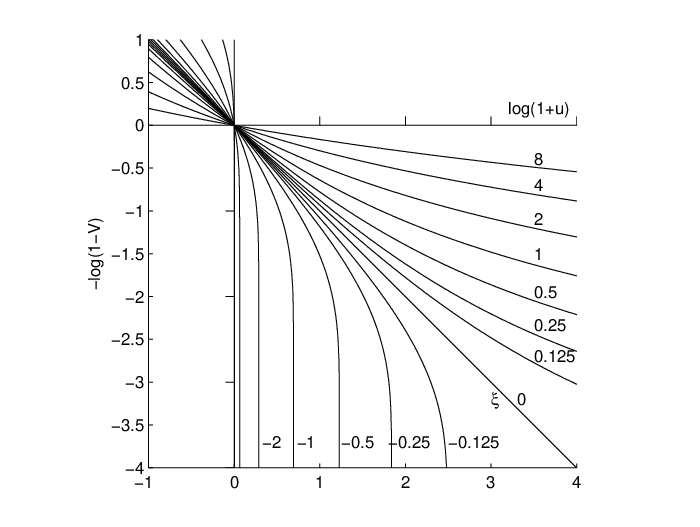
Data drawn from a GPD can now be plotted on this diagram. The data defines coordinates, via the statistic (Eqn. 2), and the ordinates are defined solely by the order index ratio (via Eqn. 8). Guided more by intuition than theorems, the general idea is that data from a GPD with tail parameter is in some sense likely to plot near to the underlying curve defined by , such that an estimate of can be obtained by, say, a simple least-squares curve fit.

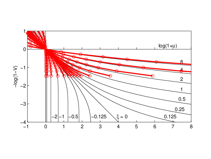


Figure 3 shows individual samples (left) and sample averages (right). The individual samples lie in the approximate vicinity of their respective curves. The sample averages (that is, the averages of over 1000 samples) follow their corresponding curves reasonably closely, although with a tendency to follow a curve at a slightly higher than that from which they were sampled. This tendency appears to reduce as the sample size is increased ( in the upper figures, and in the lower figures).
The intuitive visual representation afforded by such figures can be helpful in indicating how tail estimators applied to data drawn from more general non-GPD distributions can often lead to consistently erroneous estimates. We give an example in the Appendix, noting here only that - as we are generally trying to estimate the parameter that represents the shape of the tail - the ability of the versus construction to make visible the shape of the tail can be instructive.
Alternative plotting positions can be obtained by using , as is commonly done in QQ-plots (see for example Embrechts et al. (1999), p292). For a traditional empirical distribution function, this would correspond to the midpoint of the step at each data point. With these new plotting positions, the previous equations still apply, but with the revised definitions for the ’s included throughout.
The definition of the plotting position has a significant effect on where data is plotted. It also affects the background analytical curves. However, whilst points on a curve may move significantly, the curve as a whole moves little. Since the graphic is for illustration only, we may therefore use any to draw the background curves, but adopt the appropriate exact values when doing computations.
We shall call such diagrams the construction, and examples are shown in Figure 4. There, GPD data has been added and the averages of sampled data now plot much closer to the (re-drawn) curves of the underlying analytical approximations. We shall thus use the construction for the estimation phase, and apply a least-squares curve-fit to estimate .
(Unless stated otherwise, all further GPD samples and analysis will use .)


2.1 Curve Fitting
The ordinates are fixed by the plotting position definitions. We therefore consider the horizontal error between data and curve, defining for some function , and we choose to accord with the construction.
The sum of the squared errors over the first nine data points (the tenth data point having no error by this construction) is
| (9) |
where is the scaled data and is its analytical approximation, with .
Taking the derivative with respect to the tail parameter gives
| (10) |
The analytic approximation for the th order statistic is
| (11) |
Since we choose we have , such that error minimisation requires
| (12) |
This can be readily solved numerically for the estimate (using the Matlab function, for example)
The performance of the resulting estimator is shown in Figure 5 for samples drawn from GPDs over a range of . The left figure shows that the estimator has some variance about a very small bias, and the right figure compares the root mean square error to that of an alternative estimator - the “linearly rising” combination of elemental estimators described in McRobie (2013b). The curve-fit estimator is based on the first ten upper order statistics, together with knowledge of the twentieth. Two versions of the elemental estimator are shown in the right-hand figure. The upper curve uses knowledge of only the first ten upper order statistics, whereas the lower (more accurate) curve uses knowledge of all twenty. The curve-fit estimator nestles between the two.


Although there exist tail estimators with smaller rmse (e.g. Segers (2005)) we proceed using the curve-fit for a number of reasons. First, despite its simplicity, its performance is only marginally worse than the best available alternatives, and in many cases it is superior to other commonly-adopted procedures. For example, the curve fit works for all , not just positive (as is the case for Hill’s estimator), it does not suffer from the numerical difficulties encountered by Maximum Likelihood estimation (see for example Castillo and Daoudi (2009); McRobie (2013a)) nor does it have the convergence issues associated with MCMC Bayesian approaches applied to extremes. Secondly, only the most basic description of the curve-fit is described here and there is considerable scope for further optimisation later. Finally - and most importantly - curve-fitting brings considerable intuitive insight to the problem. This will become evident as we proceed from estimation to prediction, and especially in the case of non-GPD data.
3 Prediction in the GPD case
Having obtained an estimate of the tail parameter , a naive approach to prediction beyond the span of the data would be to extrapolate the GPD with parameter out to large extreme values. However, as is well known, this is optimistic and is liable to considerably underestimate possible future extremes. This is illustrated in Figure 6. Here, for each of 10000 samples of size drawn from a pure GPD at each of a variety of values of , the curve-fit estimate is first calculated. Predictions are then made at the recurrence levels , 50, 100, 200 and 400 using
| (13) |
with the normalised prediction given by
| (14) |
where . Here the recurrence probability of the extreme event at level is set to and for this prediction phase we return to the plotting position approximations and in line with the original basic construction.
To test each prediction, a further 10000 data points are sampled from the same distribution, and the number that exceed the prediction is counted. For each sample and its associated prediction, the exceedance probability is thus estimated as . The procedure is repeated for 10000 samples and the delivered recurrence level is estimated as . (Note: because the form of the supposedly “unknown” distribution from which data is sampled is actually known in simulations, could be evaluated analytically for each prediction. However, the numerical method is more readily adaptable and leads to results which are substantially the same).
Figure 6 shows the delivered “return period” to be generally substantially lower than the desired return level (except for at the far left - and this latter is thought to be a minor and irrelevant consequence of using the plotting positions for estimation). The wider tendency of naive extrapolation to underpredict can be readily appreciated by consideration of samples drawn from a GPD with say . For around half the samples, the tail parameter will be estimated as negative, corresponding to a bounded tail distribution, and extrapolating to rare events in the bounded tails leads to predictions which are readily overcome by further samples drawn from the true distribution.

To compensate for such underprediction, the central proposal of this paper is to predict instead from GPDs with tail parameters higher than estimated. That is, having obtained the estimate , prediction is then accomplished using , where depends on both the estimate and the desired return level . In graphical terms, having done a GPD curve-fit to the data on the construction (as per Figure 4), prediction to more extreme return levels proceeds along a curve that increases to values progressively to the right of that originally estimated. The curve so constructed corresponds, in some sense to the existence of a “predictive distribution”. Although predictive distributions are well defined in the Bayesian framework, they appear to be little used and somewhat ill-defined in frequentist settings.
3.1 The increment
Trial and error numerical experiments led to the construction of a set of curves for the increment . That is, at some given desired return level , a function was defined over the complete range of . GPD samples were generated at each over a wide range (), and for each sample, a prediction was made using the GPD with as per Eqns. 13 and 14 (but with the latter using ). The number of times the prediction was exceeded by further samples drawn from the GPD at the original was recorded, allowing the delivered recurrence level to be estimated. If fell below over particular ranges of the function was increased smoothly and locally in that general area. Typically the process began by calibrating an exponential function to get good probability matching at extreme negative and positive and then augmenting it with a set of ad hoc bump functions - broad Gaussians - in the regions of moderate . Regions of moderate and negative typically required most augmentation. The bump functions were adjusted manually until for all tested . The process was then repeated to determine the function at another recurrence level .
The resulting functions are shown in Figure 7 for five recurrence levels , 50, 100, 200, 400, these values being chosen for practical reasons. The functions have no neat analytic form.


The delivered recurrence levels of the predictor are shown in Figure 8, where it can be seen that the performance is very close to target, even for desired return levels as high as , this being a significant extrapolation from data points. Without suggesting that extrapolating far outside the data is in any way advisable, if out of sample extrapolation is to be undertaken then a method that preserves probability (such as the predictor here does to a good approximation) would appear to be more rational and less imprudent than naive extrapolation.
The predictor can also be illustrated graphically on the basic construction. The standard analytical approximation curves can be plotted for a set of . The region of the graph above the horizontal line corresponding to the return level is the region used for estimation. The corresponding extrapolation curves given by the predictor can also be added below the horizontal line. We thus obtain Figure 9.

On this graph the averages of for data sampled from GPDs at the five values of have also been plotted in red, using plotting positions. The data averages thus now plot a little to the right of the approximate analytic curves (as was seen earlier in Figure 3). To reiterate, estimation uses and prediction uses plotting positions. The addition of the data here using the convention is thus for illustration purposes only. However, the way that the prediction curves below the horizontal appear to match up so neatly with the data averages is remarkable, given that the red curves correspond to data at a specific , whilst the prediction curves are applied to data from GPDs of any . Even though, intuitively, some degree of matching may have been expected, there is as yet no explanation for this rather pleasing outcome that the prediction curves appear to be continuations of the data averages.
The procedure for making a prediction from any data set is, of course, applied computationally, and the graphic of Figure 9 is for illustration only. Nevertheless, it does show how intuitive the method is.
The way the prediction curves (thick black) veer to greater values than the naive extrapolation of the “expected” curves (thin black) is reminiscent of the behaviour of the Bayesian predictive distribution. However the prediction curves here have been obtained without reference to any prior distribution on the shape parameter. This is interesting, because there is as yet no known rational noninformative prior for the shape parameter in the three parameter GPD, and Bayesian extreme value theorists without access to any meaningful prior information may perhaps be inclined put broad normals centred loosely around . MCMC simulations also have computational issues for large predictions (associated with needing lengthy runs to populate the distant tail) whereas the procedure described here is essentially a simple function evaluation. In summary, that function evaluation is:
The algorithm has been described here in its most basic form, and there is considerable scope for further optimisation and extension. For example, only the case has been described, and extension to other values of and may be readily devised. All normalisation has been with respect to the th and th order statistics, which again, can be generalised and optimised. Also, weighted least squares estimation could be used in the curve fit (the current weights being unity for and zero for ) and alternatives may lead to reduced estimation error. Similarly, least squares is applied to the function to accord with the basic construction, but other functions may reduce estimation error.
The ultimate objective, however, is less concerned with improving parameter estimation, and more with making out-of-sample extrapolations in the general domain-of-attraction case, which we now consider.
4 Application to non-GPD data
Extreme Value Theory tells us that the upper order statistics of samples drawn from a non-GPD distribution may, with suitable scaling, in appropriate limits and under appropriate conditions, be approximated as a GPD. The non-GPD distribution is then said to be in the domain of attraction of that GPD with tail parameter , and is said to be the tail index of the non-GPD distribution. We now use this approximation to apply our GPD predictor to non-GPD data.
The strategy here is fairly obvious. Given a sample of size from a non-GPD distribution, select the upper order statistics and use least squares on the construction to make an estimate of the tail index . Then make location- and scale-invariant predictions using the GPD with tail parameter . Finally, to demonstrate that the procedure works, the performance of the predictor will be tested by seeing how often the prediction is exceeded by further data drawn from the original non-GPD distribution.
In the pure GPD case we used and extrapolated to exceedance levels , 50, 100, 200, 400, corresponding to extrapolation ratios of 1, 2.4, 4.8, 9.5 and 19. In the non-GPD case, we allow to be larger than . Predictions however will still be at the same extrapolation ratios from the 20 upper order statistics, and the recurrence levels with respect to the full sample size will be .
For data drawn from a variety of non-GPD distributions, Figures 10-12 plots the exceedence level delivered compared with that desired. In each subfigure, five curves are shown, corresponding to increasing sample size through , 60, 80, 100 to , the latter results shown by the thicker lines. For we do not expect to get good prediction performance since the predictor is constructed using half the data, which can scarcely be described as the “tail”, especially for double-sided distributions such as the normal. The key results are thus the thicker lines for , where only the upper 10 percent of the data have been used for the extrapolation.
The non-GPD distributions considered correspond to those modelled in Segers (2005). In all cases the delivered exceedance level is close to that desired, with the agreement improving for larger sample sizes. The largest extrapolation ratio shown is thus for the largest samples (of size , shown by the thicker solid lines), the uppermost prediction is to a return level of , which is over an order of magnitude beyond the return level () that would be naturally associated with the 200 data points. For such a large extrapolation, it is perhaps remarkable how closely the probability is preserved in all cases.


5 Summary
A method has been presented for making large extrapolations out-of-sample, yet in a way that gives good probability preservation. It takes a data set of size , and uses only the highest 20 upper order statistics, whose distribution is then approximated by a member of the three parameter family of GPDs. Interest in the location and scale parameters is removed by rescaling with respect to the 10th and 20th upper order statistics. The shape parameter of the domain of attraction GPD is then estimated as using a least squares curve fit (which is accompanied by a useful graphical representation). Extrapolation at any desired return level is then accomplished using a GPD with an adjusted tail parameter , where the increment is a function which has been calibrated to give good probability preservation for GPDs of any . To a good approximation this probability preservation carries over to data drawn from a wide class of non-GPD distributions.
Only the basic outline of the method has been described and there is scope for further optimisation.
References
- Castillo and Daoudi (2009) Castillo, J., Daoudi, J., 2009. Estimation of the generalized Pareto distribution. Statistics and Probability Letters 79, 684–688.
- Embrechts et al. (1999) Embrechts, P., Klüppelberg, C., Mikosch, T., 1999. Modelling Extreme Events for Insurance and Finance. Springer, Berlin.
- Mathworks (2014) Mathworks, 2014. Matlab function gpfit.
- McRobie (2013a) McRobie, F. A., 2013a. Elemental estimators for the Generalized Extreme Value tail. arXiv:1304.4362.
- McRobie (2013b) McRobie, F. A., 2013b. Elemental unbiased estimators for the Generalized Pareto tail. arXiv:1304.3918.
- McRobie (2013c) McRobie, F. A., 2013c. Probability-matching predictors for extreme extremes. arXiv:1307.7682.
- Segers (2005) Segers, J., 2005. Generalized Pickands estimators for the extreme value index. J. Stat. Planning and Inference 128 (2), 381–396.
6 Appendix: Insight into tail estimation errors for non-GPD distributions
We demonstrate briefly how the basic curve-fit construction can give insight into cases where estimators for the tail index of non-GPD distributions lead to persistently erroneous results.
Figure 13 compares the root mean square errors (RMSE) of three tail index estimators applied to the upper order statistics of samples of size from a wide range of distributions. The three estimators are the unconstrained Segers estimator (Segers (2005)), the linearly rising combination of elemental estimators (McRobie (2013b)) and the Maximum Likelihood estimate of the Matlab gpfit function (Mathworks (2014)). As increases, the RMSE in almost the all non-GPD cases shows initial improvements before diverging again as approaches . In almost all cases, the Segers estimator has RMSE lower than the other two (the GPD (lower left) being one exception). However, a focus on RMSE alone does not explain what is happening here. We focus on the case centre left, the Weibull distribution, this being an example where all estimators are performing rather poorly.


Figure 14 shows the unconstrained Segers tail index estimates for the Weibull, plotting mean standard deviation. The theoretical answer for a Weibull is . The estimator has been applied to the first upper order statistics of samples of size . (The corresponding plot for the other two estimators are decidedly similar, with estimates lying just above those of the Segers estimator.) It can be seen that, as increases, the reductions in RMSE that are associated with the reduced variance of working with more data points are soon outweighed by the increased bias as approaches the full sample size .
However, Figure 14 suggests that the question of which estimator has the marginally better RMSE is perhaps of lesser interest than the question as to why all the estimates are so far from the correct value. Although the true answer is , all the estimators seems fairly convinced that is actually positive.
That an extreme value estimator performs badly for the Weibull distribution is perhaps surprising, given the comparative ubiquity of Weibulls in the extreme value literature. Weibulls are commonly applied in reliability analysis, such as to the failure rates of components. Also, there is a form of the Weibull inherent in the family of Generalised Extreme Value distributions, although this is the reversed- or EV-Weibull (for which tail index estimators work rather well).

Some insight into why the estimators perform so badly on the (unreversed) Weibull can be obtained by plotting Weibull information onto the graphical construction of the main body of this paper.
The distribution function of the three-parameter Weibull may be written
| (15) |
Inversion of the tail distribution function, as was done for the GPD, leads to the analytical approximation
| (16) |
In Figure 15, these analytical approximations are plotted onto the construction for for the three cases 100 and 200.

The insight afforded by the construction is now apparent. The plot makes visible the way that the tail is “pulled in” towards the true solution as is decreased. Even by eye, the picture suggests that a GPD-based tail estimator would be expected to fall from a value just below 1.0 for to a value near 0.25 for . Applying least squares to the analytical approximations gives a slightly more precise view of what should be anticipated when a GPD predictor is applied to Weibull data: the tail estimates should be expected to be around , 0.51 and 0.93 for , 100 and 200 respectively. The performance of the unconstrained Segers estimator (Figure 14) is decidedly similar.
Averages of data sampled from Weibulls have also been plotted (in red) onto Figure 15, and these lie close to the analytical approximations. The analytical approximations, though, are the important information here, having been made a priori, without sampling. If the analytical form of a non-GPD distribution is known, then the basic construction allows the erroneous estimates that a GPD-based estimator may make to be largely anticipated a priori in a highly visual and intuitive manner.
6.1 Corollary - a tail estimator for non-GPD data
Given that the basic construction shows how tail estimates may change under increasing for non-GPD data, it suggests that such changes may be monitored to assess just how non-GPD the data is, leading to the possibility of improved estimates.
For example, at any one could make a sequence of curve fit estimates at a sequence of which increase to and look at how the tail is pulled in as increases. Some careful back-extrapolation of the back to the hypothetical value may thus lead to reduced bias in the level estimate.
Figure 15 gives the visual insight. There, the sequence of progressively smaller leads to a sequence of curves that approach the true value . When using , is the analyst supposed to accept an estimate , even though those 200 data points contain within them the data which is suggesting ? Thus when using , rather than merely accepting the direct estimate of or even the estimate of , a value lower than 0.25 appears to be reasonable. This could be estimated by back-extrapolation of the various estimates back to the hypothetical intercept. Of course, Figure 15 shows averages, whereas the procedure would need to be applied to individual samples and the back-extrapolation results would be complicated by the associated scatter.
A simple procedure is outlined here for demonstration purposes only. For a sample of size , for any , we can pick the length-eight sequence at the eighth points of . We can then construct eight curve-fit estimates, using only the first order statistics normalised with respect to the th and th values (and using the plotting positions ). The eight estimates corresponding to the eight can then be extrapolated back to the hypothetical intercept by least squares fitting of a straight line (and, for this example, we choose to apply weights proportional to to give more weight to larger ). The resulting estimates for the Weibull with are shown in Figure 16.
Segers (2005) proposed two versions of his tail index estimator. The unconstrained version was based heavily on the GPD, and was thus prone to substantial bias when applied to non-GPD data (as shown by Figure 14). The more sophisticated constrained version endeavoured to remove this bias by, loosely speaking, attempting to measure how non-GPD the data was and compensate accordingly. There is an obvious parallel with the and curve-fit estimators here. The simple -based curve-fit is constructed for the GPD, and the estimator that uses the sequence of endeavours to compensate for non-GPD behaviour.
Figure 16 shows the corresponding performances of the unconstrained/constrained Segers and the curve fit estimators to be strikingly similar. The lower part of the Figure shows the RMSE results for the enhanced estimators that have endeavoured to compensate for non-GPD behaviour. Considering the simplicity of the curve fit approach, the close correspondence is perhaps surprising.


The example was for illustration only. On some distributions (e.g. the normal) the constrained Segers gives lower RMSE than the curve-fit, but on others (e.g. the (2,2) Beta distribution) the curve-fit sequence is arguably the better. Although there is scope for further optimisation of the estimator, the intention here was never to create a better tail index estimator, but to show how the curve-fit gives insight. The emphasis of the main body of the paper is on prediction: estimation is of lesser importance, especially since prediction is done using only the information, and at even the highly sophisticated constrained Segers estimator tends to give considerably worse RMSE than many simpler alternatives.