跳到论文正文
W Papers独立论文阅读器 arXiv:1408.1286 论文正文 计算阅读时间 · 0%
引用这篇论文根据当前论文元数据生成,正式投稿前建议核对。


License: arXiv.org perpetual non-exclusive license
arXiv:1408.1286v1 [math.NA] 06 Aug 2014

Superconvergence of both the Crouzeix–Raviart and Morley elementsThanks: The first author was supported by the NSFC Project 11271035 and by the NSFC Key Project 11031006.

Jun Hu∗ Address: ∗ LMAM and School of Mathematical Sciences, Peking University, Beijing 100871, P. R. China Email address: hujun@math.pku.edu.cn and Rui Ma† Address: † LMAM and School of Mathematical Sciences, Peking University, Beijing 100871, P. R. China Email address: maruipku@gmail.com
Abstract.

In this paper, a new method is proposed to prove the superconvergence of both the Crouzeix–Raviart and Morley elements. The main idea is to fully employ equivalences with the first order Raviart–Thomas element and the first order Hellan–Herrmann–Johnson element, respectively. In this way, some special conformity of discrete stresses is explored and superconvergence of mixed elements can be used to analyze superconvergence of nonconforming elements. Finally, a half order superconvergence by postprocessing is proved for both nonconforming elements.

Key words and phrases: 
Superconvergence, Crouzeix-Raviart element, Morley element
AMS Subject Classification: 65N30, 65N15, 35J25

1. Introduction

The superconvergence analysis is well studied for conforming finite elements, see [7, 19], and as well as mixed finite elements of second order problems. For triangular mixed elements, Douglas et al. [12] proved superconvergence for the displacement variable on general triangulations, see also [1]. Brandts [4, 5] proved superconvergence for the stress variable on uniform triangulations for the first and second order Raviart–Thomas elements [26], respectively. For superconvergence along the Gauss–lines in rectangular mixed finite element methods, see [13]. However, in the case of nonconforming finite elements, due to the reduced continuity of trial and test functions, it becomes much more difficult to establish superconvergence properties and related asymptotic error expansions. There are several superconvergence results on rectangular elements. In [9, 28], for the Wilson element [2], the superconvergence estimate of the gradient error on the centers of elements was obtained. The essential point employed therein is that the Wilson element space can be split into a conforming part and a nonconforming part. Thanks to the superconvergence estimate of the consistency error, some superconvergence results of the nonconforming rotated Q1Q_{1} element [25] and its variants were derived, see [14, 18, 23]. As for the plate bending problem, there are only few superconvergence results for nonconforming finite elements. In [8], Chen first established the supercloseness of the corrected interpolation of the incomplete biquadratic element [27] on uniform rectangular meshes. By using similar corrected interpolations as in [8], Mao et al. [21] first proved a half order superconvergence for the Morley element [24] and the incomplete biquadratic nonconforming element on uniform rectangular meshes. Based on the equivalence to the Stokes equations and a superconvergence result of Ye [30] on the Crouzeix–Raivart element [11], Huang et al. [15] derived the superconvergence for the Morley element, which was postprocessed by projecting the finite element solution to another finite element space on a coarser mesh [29].

In this paper, a new method is proposed to derive the superconvergence for nonconforming finite elements. The main idea is to explore some conformity of discrete stresses produced by nonconforming methods. Note that such conformity can not be obtained within original formulations for nonconforming elements. Fortunately, for the Crouzeix–Raviart element of the Poisson problem and the Morley element of the plate bending problem, it can be deduced by using the equivalences with the first order Raviart–Thomas element [22] and the first order Hellan–Herrmann-Johnson element [1], respectively. More precisely, based on these equivalences, we can translate the problem of superconvergence of nonconforming elements to the problem of superconvergence of mixed elements. Note that mixed elements are conforming methods within mixed formulations. This enables us to use superconvergence of mixed elements to establish superconvergence of nonconforming elements. In this way, it is able to overcome the main difficulty caused by nonconformity for the superconvergence analysis of nonconforming finite elements. In particular, a half order superconvergence by postprocessing is proved for both aforementioned two nonconforming elements on uniform triangulations. As a byproduct, the superconvergence is establised for the Hellan–Herrmann-Johnson element which is somehow missing in literature. Numerical tests are provided to demonstrate theoretical results.

The remaining paper is organized as follows. Section 2 proposes the Poisson problem and the corresponding nonconforming and mixed finite elements. Section 3 presents the superconvergence result for the Raviart–Thomas element and proves the superconvergence result for the Crouzeix–Raviart element. Section 4 proposes the plate bending problem and the corresponding nonconforming and mixed finite elements. Section 5 proves the superconvergence result for the Hellan–Herrmann–Johnson element and the Morley element. Section 6 presents some numerical tests.

2. The Poisson problem and its Crouzeix–Raviart element

Throughout this paper, let Ω⊂ℝ2\Omega\subset\mathbb{R}^{2} be a polygonal domain. We recall some notations for Sobolev spaces (see [10]). For a subdomain GG of Ω\Omega, let Pm​(G)P_{m}(G) be the space of polynomials of degree less than or equal to mm over GG. Hs​(G)H^{s}(G) denotes the classical Sobolev space with norm ∥⋅∥s,G\|\cdot\|_{s,G} and the seminorm |⋅|s,G|\cdot|_{s,G}. Wk,∞​(G)W^{k,\infty}(G) denotes the classical Sobolev space with norm ∥⋅∥k,∞,G\|\cdot\|_{k,\infty,G} and the seminorm |⋅|k,∞,G|\cdot|_{k,\infty,G}.

Given f∈L2​(Ω)f\in L^{2}(\Omega), the Poisson model problem finds u∈H01​(Ω)u\in H^{1}_{0}(\Omega) such that

(2.1) (∇u,∇v)=(f,v) for all ​v∈H01​(Ω).(\nabla u,\nabla v)=(f,v)\quad\text{ for all }v\in H^{1}_{0}(\Omega).

By introducing an auxiliary variable σ:=∇u\sigma:=\nabla u, the problem can be formulated as the following equivalent mixed problem which seeks (σ,u)∈H⁡(div,Ω)×L2​(Ω)(\sigma,u)\in H(\operatorname{div},\Omega)\times L^{2}(\Omega) such that

(2.2) (σ,τ)+(u,div⁡τ)=0 for any ​τ∈H⁡(div,Ω),(div⁡σ,v)=(−f,v) for any ​v∈L2​(Ω).\begin{split}&(\sigma,\tau)+(u,\operatorname{div}\tau)=0\quad\text{ for any }\tau\in H(\operatorname{div},\Omega),\\ &(\operatorname{div}\sigma,v)=(-f,v)\quad\text{ for any }v\in L^{2}(\Omega).\end{split}

Suppose that Ω¯\bar{\Omega} is covered by uniform shape regular triangulations 𝒯\mathcal{T} consisting of triangles in two dimensions. 𝒯\mathcal{T} is said to be uniform if any two adjacent triangles of 𝒯\mathcal{T} form a parallelogram. hh denotes the diameter of the element K∈𝒯K\in\mathcal{T}. Let ℰ\mathcal{E} denote the set of edges of 𝒯\mathcal{T}, and ℰ⁡(Ω)\mathcal{E}(\Omega) denote the set of all the interior edges, and ℰ⁡(∂Ω)\mathcal{E}(\partial\Omega) denote the set of all the boundary edges. Given e∈ℰe\in\mathcal{E}, let νe\nu_{e} be the unit normal vector of ee and [⋅][\cdot] be jumps of piecewise functions over ee, namely

[v]:=v|K+−v|K−[v]:=v|_{K^{+}}-v|_{K^{-}}

for piecewise functions vv and any two elements K+K^{+} and K−K^{-} which share the common edge ee. Note that [⋅][\cdot] becomes traces of functions on ee for boundary edges ee. Throughout the paper, an inequality A≲BA\lesssim B replaces A≤C​BA\leq CB with some multiplicative mesh–size independent constant C>0C>0 .

The Crouzeix–Raviart element [11] space over 𝒯\mathcal{T} is defined by

WCR:={v∈L2(Ω):v|K∈P1(K) for each K∈𝒯,∫e[v]ds=0 for all e∈ℰ(Ω)},W_{\rm CR}:=\begin{array}[t]{l}\big\{v\in L^{2}(\Omega):v|_{K}\in P_{1}(K)\text{ for each }K\in\mathcal{T},\int_{e}[v]ds=0\text{ for all }e\in\mathcal{E}(\Omega)\big\}\,,\end{array}
VCR:={v∈WCR:∫ev​ds=0​ for all ​e∈ℰ⁡(∂Ω)}.V_{\rm CR}:=\begin{array}[t]{l}\big\{v\in W_{\rm CR}:\int_{e}vds=0\text{ for all }e\in\mathcal{E}(\partial\Omega)\big\}\,.\end{array}

The Crouzeix–Raviart element method of Problem (2.1) finds uCR∈VCRu_{\rm CR}\in V_{\rm CR} such that

(2.3) (∇NCuCR,∇NCv)=(f,v)​ for all ​v∈VCR.(\nabla_{\rm NC}u_{\rm CR},\nabla_{\rm NC}v)=(f,v)\text{ for all }v\in V_{\rm CR}.

To analyze the superconvergence of the Crouzeix–Raviart element, we introduce the first order Raviart–Thomas element [26] whose shape function space is

RT⁡(K):=(P0​(K))2+x​P0​(K)​ for any ​K∈𝒯.{\rm RT}(K):=(P_{0}(K))^{2}+xP_{0}(K)\text{ for any }K\in\mathcal{T}.

Then the corresponding global finite element space reads

(2.4) RT⁡(𝒯):={τ∈H⁡(div,Ω):τ|K∈RT⁡(K)​ for any ​K∈𝒯}.{\rm RT}(\mathcal{T}):=\{\tau\in H(\operatorname{div},\Omega):\tau|_{K}\in{\rm RT}(K)\text{ for any }K\in\mathcal{T}\}.

To get a stable pair of space, the piecewise constant space is proposed to approximate the displacement, namely,

(2.5) URT​(𝒯):={v∈L2​(Ω):v|K∈P0​(K)​ for any ​K∈𝒯}.{\rm U}_{\rm RT}(\mathcal{T}):=\{v\in L^{2}(\Omega):v|_{K}\in P_{0}(K)\text{ for any }K\in\mathcal{T}\}.

The Raviart–Thomas element method of Problem (2.2) seeks (σRT,uRT)∈RT⁡(𝒯)×URT​(𝒯)(\sigma_{\rm RT},u_{\rm RT})\in{\rm RT}(\mathcal{T})\times{\rm U}_{\rm RT}(\mathcal{T}) such that

(2.6) (σRT,τ)+(uRT,div⁡τ)=0 for any ​τ∈RT⁡(𝒯),(div⁡σRT,v)=(−f,v) for any ​v∈URT​(𝒯).\begin{split}&(\sigma_{\rm RT},\tau)+(u_{\rm RT},\operatorname{div}\tau)=0\quad\text{ for any }\tau\in{\rm RT}(\mathcal{T}),\\ &(\operatorname{div}\sigma_{\rm RT},v)=(-f,v)\quad\text{ for any }v\in{\rm U}_{\rm RT}(\mathcal{T}).\end{split}

Given K∈𝒯K\in\mathcal{T} and f∈L2​(K)f\in L^{2}(K), define fK=1|K|​∫Kf​𝑑xf_{K}=\frac{1}{|K|}\int_{K}fdx. Given f∈L2​(Ω)f\in L^{2}(\Omega), define the piecewise constant projection Π0​f\Pi_{0}f by

(Π0​f)|K=fK.(\Pi_{0}f)|_{K}=f_{K}.

Because of the definition of URT​(𝒯){\rm U}_{\rm RT}(\mathcal{T}), ff in the second equation of (2.6) can be replaced by Π0​f\Pi_{0}f. We define the auxiliary method: Find u¯CR∈VCR\bar{u}_{\rm CR}\in V_{\rm CR} such that

(2.7) (∇NCu¯CR,∇NCv)=(Π0​f,v)​ for all ​v∈VCR.(\nabla_{\rm NC}\bar{u}_{\rm CR},\nabla_{\rm NC}v)=(\Pi_{0}f,v)\text{ for all }v\in V_{\rm CR}.

Note that this method differs from (2.3) only by the presence of the projection in the right hand side. Marini [22] proved its equivalence to the Raviart–Thomas element method (2.6):

(2.8) σRT|K=∇u¯CR|K−fK2​(x−Mid⁡(K))x∈K​ for any K∈𝒯,\sigma_{\rm RT}|_{K}=\nabla\bar{u}_{\rm CR}|_{K}-\frac{f_{K}}{2}(x-{\rm Mid(K)})\quad x\in K\text{ for any $K\in\mathcal{T}$},

where Mid⁡(K){\rm Mid}(K) denotes the center of KK.

Subtracting (2.7) from (2.3) with v=uCR−u¯CRv=u_{\rm CR}-\bar{u}_{\rm CR} yields that

(∇NC(uCR−u¯CR),∇NC(uCR−u¯CR))=(f−Π0​f,uCR−u¯CR)=(f−Π0​f,uCR−u¯CR−Π0​(uCR−u¯CR)).\begin{split}(\nabla_{\rm NC}(u_{\rm CR}-\bar{u}_{\rm CR}),\nabla_{\rm NC}(u_{\rm CR}-\bar{u}_{\rm CR}))&=(f-\Pi_{0}f,u_{\rm CR}-\bar{u}_{\rm CR})\\ &=(f-\Pi_{0}f,u_{\rm CR}-\bar{u}_{\rm CR}-\Pi_{0}(u_{\rm CR}-\bar{u}_{\rm CR})).\end{split}

Hence, the Poincare´\acute{\rm e} inequality from [17] yields

(2.9) ‖∇NC(uCR−u¯CR)‖0,Ω≤h2j1,12​|f|1,Ω,\|\nabla_{\rm NC}(u_{\rm CR}-\bar{u}_{\rm CR})\|_{0,\Omega}\leq\frac{h^{2}}{j^{2}_{1,1}}|f|_{1,\Omega},

where j1,1=3.8317j_{1,1}=3.8317 denotes the first positive root of the Bessel function of the first kind.

3. Superconvergence analysis of the Crouzeix–Raviart element

In this section, we first present the superconvergence result of the Raviart–Thomas element by Brandts [4]. Then, based on this result and the equivalence (2.8), we derive the superconvergence result of the Crouzeix–Raviart element.

3.1. The superconvergence result of the Raviart–Thomas element

We introduce a result on Sobolev spaces in the following lemma, which describes the behavior of functions near the boundary. Define Ωh\Omega_{h} as the subset of points in Ω\Omega having distance less that hh from the boundary:

Ωh={x∈Ω:∃y∈∂Ω,dist(x,y)≤h}.\Omega_{h}=\{x\in\Omega:\exists y\in\partial\Omega,{\rm dist}(x,y)\leq h\}.

Then we have the following result, see [4, 20].

Lemma 3.1.

For v∈Hs​(Ω)v\in H^{s}(\Omega), where 0≤s≤120\leq s\leq\frac{1}{2}, we have

‖v‖0,Ωh≲hs​‖v‖s,Ω.\|v\|_{0,\Omega_{h}}\lesssim h^{s}\|v\|_{s,\Omega}.

Given q∈(H1​(Ω))2q\in(H^{1}(\Omega))^{2}, define the interpolation operator ΠRT​q∈RT⁡(𝒯)\Pi_{\rm RT}q\in{\rm RT}(\mathcal{T}) by

∫e(ΠRT​q−q)T​νe​𝑑s=0for all ​e∈ℰ.\int_{e}(\Pi_{\rm RT}q-q)^{T}\nu_{e}ds=0\quad\text{for all }e\in\mathcal{E}.

Brandts gave the following superconvergence result of the Raviart–Thomas element, see [4, Theorem 3.2] .

Theorem 3.2.

Let σ∈(H2​(Ω))2\sigma\in(H^{2}(\Omega))^{2} and σR​T\sigma_{RT} be the solutions of (2.2) and (2.6), respectively. There holds that

‖σRT−ΠRT​σ‖0,Ω≲h32​(‖σ‖32,Ω+h12​|σ|2,Ω).\|\sigma_{\rm RT}-\Pi_{\rm RT}\sigma\|_{0,\Omega}\lesssim h^{\frac{3}{2}}(\|\sigma\|_{\frac{3}{2},\Omega}+h^{\frac{1}{2}}|\sigma|_{2,\Omega}).

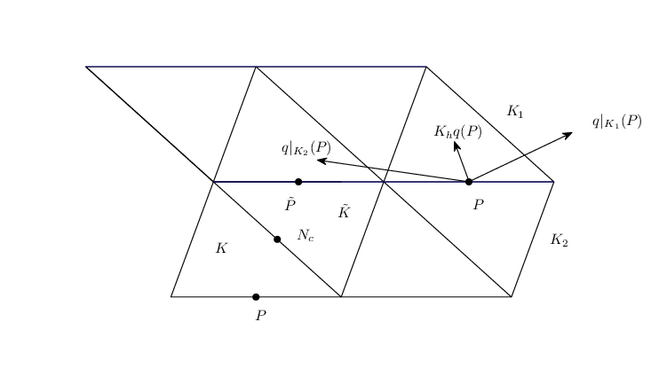
Furthermore, a post-processing mechanism was proposed in [4], which when applied to the projection ΠRT​q\Pi_{\rm RT}q of a function q∈(H2​(Ω))2q\in(H^{2}(\Omega))^{2}, will improve its approximation property. Given q∈RT⁡(𝒯)q\in{\rm RT}(\mathcal{T}), define function Kh​q∈(WCR)2K_{h}q\in(W_{\rm CR})^{2} as follows (see also Figure 1).

Refer to caption
Figure 1. Post-processing a function q∈RT⁡(𝒯)q\in{\rm RT}(\mathcal{T})
  • •

    Given e∈ℰ⁡(Ω)e\in\mathcal{E}(\Omega), suppose that e=K1∩K2e=K_{1}\cap K_{2} and PP denotes the center of ee. Let

    Kh​q​(P)=12​(q|K1​(P)+q|K2​(P)).K_{h}q(P)=\frac{1}{2}(q|_{K_{1}}(P)+q|_{K_{2}}(P)).
  • •

    Given e∈ℰ⁡(∂Ω)e\in\mathcal{E}(\partial\Omega) and e⊂∂Ke\subset\partial K, there exists at least one K~∈𝒯\tilde{K}\in\mathcal{T} such that N=K∪K~N=K\cup\tilde{K} is a parallelogram. The straight line through the center PP of ee and the center NcN_{c} of the parallelogram intersects the boundary of NN in another point P~\tilde{P}. Define

    Kh​q​(P)=2​Kh​q​(Nc)−Kh​q​(P~).K_{h}q(P)=2K_{h}q(N_{c})-K_{h}q(\tilde{P}).

Brandts [4] proved that the vector Kh​ΠRT​qK_{h}\Pi_{\rm RT}q is a higher order approximation of qq than ΠRT​q\Pi_{\rm RT}q itself.

Theorem 3.3.

Suppose q∈(H2​(Ω))2q\in(H^{2}(\Omega))^{2}, then there holds that

‖q−Kh​ΠRT​q‖0,Ω≲h2​|q|2,Ω.\|q-K_{h}\Pi_{\rm RT}q\|_{0,\Omega}\lesssim h^{2}|q|_{2,\Omega}.

Combining Theorem 3.2 and Theorem 3.3 concludes that the post-processing operator KhK_{h} also improves the order of approximation of σRT\sigma_{\rm RT}.

Corollary 3.4.

Let σ∈(H2​(Ω))2\sigma\in(H^{2}(\Omega))^{2} and σR​T\sigma_{RT} be the solutions of (2.2) and (2.6), respectively. There holds that

‖σ−Kh​σRT‖0,Ω≲h32​(‖σ‖32,Ω+h12​|σ|2,Ω).\|\sigma-K_{h}\sigma_{\rm RT}\|_{0,\Omega}\lesssim h^{\frac{3}{2}}(\|\sigma\|_{\frac{3}{2},\Omega}+h^{\frac{1}{2}}|\sigma|_{2,\Omega}).

3.2. The superconvergence result of the Crouzeix–Raviart element

Theorem 3.5.

Let u∈H3​(Ω)u\in H^{3}(\Omega) and uCRu_{\rm CR} be the solutions of (2.1) and (2.3), respectively. Further, suppose that f∈W1,∞​(Ω)f\in W^{1,\infty}(\Omega), then we have

(3.1) ‖∇u−Kh​∇NCuCR‖0,Ω≲h32​(‖u‖52,Ω+h12​|u|3,Ω+h12|​f|1,∞,Ω).\|\nabla u-K_{h}\nabla_{\rm NC}u_{\rm CR}\|_{0,\Omega}\lesssim h^{\frac{3}{2}}(\|u\|_{\frac{5}{2},\Omega}+h^{\frac{1}{2}}|u|_{3,\Omega}+h^{\frac{1}{2}}|f|_{1,\infty,\Omega}).
Proof.

Using the equivalence equality (2.8), for e=K1∩K2e=K_{1}\cap K_{2} and the center PP of ee, there holds that

|Kh​(∇NCu¯CR−σRT)​(P)|=|fK14​(P−Mid⁡(K1))+fK24​(P−Mid⁡(K2))||K_{h}(\nabla_{\rm NC}\bar{u}_{\rm CR}-\sigma_{\rm RT})(P)|=|\frac{f_{K_{1}}}{4}(P-{\rm Mid}(K_{1}))+\frac{f_{K_{2}}}{4}(P-{\rm Mid}(K_{2}))|

Since K1K_{1} and K2K_{2} form a parallelogram, we have P−Mid⁡(K1)=Mid⁡(K2)−PP-{\rm Mid}(K_{1})={\rm Mid}(K_{2})-P. This yields that

|Kh​(∇NCu¯CR−σRT)​(P)|=14​|(fK1−fK2)​(P−Mid⁡(K1))|≲h2​|f|1,∞,Ω.\begin{split}|K_{h}(\nabla_{\rm NC}\bar{u}_{\rm CR}-\sigma_{\rm RT})(P)|&=\frac{1}{4}|(f_{K_{1}}-f_{K_{2}})(P-{\rm Mid}(K_{1}))|\\ &\lesssim h^{2}|f|_{1,\infty,\Omega}.\end{split}

Suppose that ϕi,1≤i≤3\phi_{i},1\leq i\leq 3 denote the nodal basis functions on KK of (WCR)2(W_{\rm CR})^{2}. Hence, by the definition of KhK_{h} and scaling arguments, there holds that

‖Kh​(∇NCu¯CR−σRT)‖0,K2≲h4​|f|1,∞,Ω2​∑i=13‖ϕi‖0,K2≲h6​|f|1,∞,Ω2.\|K_{h}(\nabla_{\rm NC}\bar{u}_{\rm CR}-\sigma_{\rm RT})\|^{2}_{0,K}\lesssim h^{4}|f|_{1,\infty,\Omega}^{2}\sum_{i=1}^{3}\|\phi_{i}\|^{2}_{0,K}\lesssim h^{6}|f|_{1,\infty,\Omega}^{2}.

Summing over all triangles K∈𝒯K\in\mathcal{T} gives that

(3.2) ‖Kh​(∇NCu¯CR−σRT)‖0,Ω≲h2​|f|1,∞,Ω.\begin{split}\|K_{h}(\nabla_{\rm NC}\bar{u}_{\rm CR}-\sigma_{\rm RT})\|_{0,\Omega}\lesssim h^{2}|f|_{1,\infty,\Omega}.\end{split}

Since ∇NCu¯CR−∇NCuCR\nabla_{\rm NC}\bar{u}_{\rm CR}-\nabla_{\rm NC}u_{\rm CR} is a piecewise constant, the inverse estimate and (2.9) yield that

(3.3) ‖Kh​(∇NCu¯CR−∇NCuCR)‖0,Ω≲‖∇NC(u¯CR−uCR)‖0,Ω≲h2​|f|1,Ω≲h2​|f|1,∞,Ω.\|K_{h}(\nabla_{\rm NC}\bar{u}_{\rm CR}-\nabla_{\rm NC}u_{\rm CR})\|_{0,\Omega}\lesssim\|\nabla_{\rm NC}(\bar{u}_{\rm CR}-u_{\rm CR})\|_{0,\Omega}\lesssim h^{2}|f|_{1,\Omega}\lesssim h^{2}|f|_{1,\infty,\Omega}.

The triangle inequality plus Corollary 3.4, (3.2) and (3.3) complete the proof. ∎

4. The plate bending problem and its Morley element

Given f∈L2​(Ω)f\in L^{2}(\Omega), the plate bending model problem finds u∈H02​(Ω)u\in H^{2}_{0}(\Omega) such that

(4.1) (∇2u,∇2v)=(f,v)for all ​v∈H02​(Ω).(\nabla^{2}u,\nabla^{2}v)=(f,v)\quad\text{for all }v\in H^{2}_{0}(\Omega).

Given any space VV, we define (V)s4(V)^{4}_{\rm s} as follows:

(V)s4:={τ=(τi​j),1≤i≤j≤2:τi​j∈V,τ12=τ21}.(V)^{4}_{\rm s}:=\{\tau=(\tau_{ij}),1\leq i\leq j\leq 2:\tau_{ij}\in V,\tau_{12}=\tau_{21}\}.

Given K∈𝒯K\in\mathcal{T}, ν\nu denotes the unit outward normal to ∂K\partial K and tt the unit tangent to ∂K\partial K. Given τ∈(H1​(K))s4\tau\in(H^{1}(K))^{4}_{\rm s}, we set

Mν​ν​(τ)\displaystyle M_{\nu\nu}(\tau) =\displaystyle= νT​τ​ν,\displaystyle\nu^{T}\tau\nu,
Mν​t​(τ)\displaystyle M_{\nu t}(\tau) =\displaystyle= νT​τ​t.\displaystyle\nu^{T}\tau t.

By introducing an auxiliary variable σ:=∇2u\sigma:=\nabla^{2}u, the mixed formulation of (4.1) seeks (σ,u)∈S×D(\sigma,u)\in S\times D, see [16],

(4.2) (σ,τ)+∑K∈𝒯−(τ,∇2u)L2​(K)+∫∂KMν​ν(τ)∂u∂νds=0 for any τ∈S,∑K∈𝒯−(σ,∇2v)L2​(K)+∫∂KMν​ν(σ)∂v∂νds=(−f,v) for any v∈D,\begin{split}&(\sigma,\tau)+\sum_{K\in\mathcal{T}}-(\tau,\nabla^{2}u)_{L^{2}(K)}+\int_{\partial K}M_{\nu\nu}(\tau)\frac{\partial u}{\partial\nu}ds=0\quad\text{ for any }\tau\in S,\\ &\sum_{K\in\mathcal{T}}-(\sigma,\nabla^{2}v)_{L^{2}(K)}+\int_{\partial K}M_{\nu\nu}(\sigma)\frac{\partial v}{\partial\nu}ds=(-f,v)\quad\text{ for any }v\in D,\end{split}

where

S={τ∈(L2(Ω))4s:τ|K∈(H1(K))4s for all K∈𝒯, and Mν​ν(τ) is continuous across interelement edges},D={v∈H01​(Ω):v|K∈H2​(K)​ for all ​K∈𝒯}.\begin{split}S=&\{\tau\in(L^{2}(\Omega))^{4}_{\rm s}:\tau|_{K}\in(H^{1}(K))^{4}_{\rm s}\text{ for all }K\in\mathcal{T},\\ &\text{ and }M_{\nu\nu}(\tau)\text{ is continuous across interelement edges}\},\\ D=&\{v\in H^{1}_{0}(\Omega):v|_{K}\in H^{2}(K)\text{ for all }K\in\mathcal{T}\}.\end{split}

The Morley element space [24] VMV_{\rm M} over 𝒯\mathcal{T} is defined by

VM:={v∈L2​(Ω):v|K∈P2​(K)​ for each ​K∈𝒯,v​ is continuous at eachinterior vertex and vanishes on each boundary vertex,∫e[∂v∂νe]ds=0for all e∈ℰ(Ω), and ∫e∂v∂νeds=0 for all e∈ℰ(∂Ω)}.\begin{split}V_{\rm M}:=\big\{&v\in L^{2}(\Omega):v|_{K}\in P_{2}(K)\text{ for each }K\in\mathcal{T},v\text{ is continuous at each}\\ &\text{interior vertex and vanishes on each boundary vertex},\int_{e}[\frac{\partial v}{\partial\nu_{e}}]ds=0\\ &\text{for all }e\in\mathcal{E}(\Omega),\text{ and }\int_{e}\frac{\partial v}{\partial\nu_{e}}ds=0\text{ for all }e\in\mathcal{E}(\partial\Omega)\big\}.\end{split}

The Morley element method of Problem (4.1) finds uM∈VMu_{\rm M}\in V_{\rm M} such that

(4.3) (∇NC2uM,∇NC2v)=(f,v)for all ​v∈VM.(\nabla^{2}_{\rm NC}u_{\rm M},\nabla^{2}_{\rm NC}v)=(f,v)\quad\text{for all }v\in V_{\rm M}.

To analyze the superconvergence of the Morley element, we introduce the first order Hellan–Herrmann–Johnson element [16]. Define

HHJ⁡(𝒯)={τ∈S:τ|K∈(P0​(K))s4​ for any ​K∈𝒯},UHHJ​(𝒯)={v∈H01​(Ω):v|K∈P1​(K)​ for any ​K∈𝒯}.\begin{split}{\rm HHJ}(\mathcal{T})=&\{\tau\in S:\tau|_{K}\in(P_{0}(K))^{4}_{\rm s}\text{ for any }K\in\mathcal{T}\},\\ {\rm U}_{\rm HHJ}(\mathcal{T})=&\{v\in H^{1}_{0}(\Omega):v|_{K}\in P_{1}(K)\text{ for any }K\in\mathcal{T}\}.\end{split}

The first order Hellan–Herrmann–Johnson element of Problem (4.2) finds (σHHJ,uHHJ)∈HHJ⁡(𝒯)×UHHJ​(𝒯)(\sigma_{\rm HHJ},u_{\rm HHJ})\in{\rm HHJ}(\mathcal{T})\times{\rm U}_{\rm HHJ}(\mathcal{T}) such that

(4.4) (σHHJ,τ)+∑K∈𝒯∫∂KMν​ν​(τ)​∂uHHJ∂ν​ds=0 for any ​τ∈HHJ⁡(𝒯),∑K∈𝒯∫∂KMν​ν​(σHHJ)​∂v∂ν​ds=(−f,v) for any ​v∈UHHJ​(𝒯).\begin{split}&(\sigma_{\rm HHJ},\tau)+\sum_{K\in\mathcal{T}}\int_{\partial K}M_{\nu\nu}(\tau)\frac{\partial u_{\rm HHJ}}{\partial\nu}ds=0\quad\text{ for any }\tau\in{\rm HHJ}(\mathcal{T}),\\ &\sum_{K\in\mathcal{T}}\int_{\partial K}M_{\nu\nu}(\sigma_{\rm HHJ})\frac{\partial v}{\partial\nu}ds=(-f,v)\quad\text{ for any }v\in{\rm U}_{\rm HHJ}(\mathcal{T}).\end{split}

Given v∈H02​(Ω)∪VMv\in H^{2}_{0}(\Omega)\cup V_{\rm M}, define the interpolation operator ΠD:H02​(Ω)∪VM→UHHJ​(𝒯)\Pi_{\rm D}:H^{2}_{0}(\Omega)\cup V_{\rm M}\rightarrow{\rm U}_{\rm HHJ}(\mathcal{T}) by

(4.5) ΠD​v​(z)=v⁡(z)​ for each vertex z of ​𝒯.\Pi_{\rm D}v(z)=v(z)\text{ for each vertex $z$ of }\mathcal{T}.

Hence, we introduce the auxiliary method: The modified Morley element finds u¯M∈VM\bar{u}_{\rm M}\in V_{\rm M} such that

(4.6) (∇NC2u¯M,∇NC2v)=(f,ΠD​v)for all ​v∈VM.(\nabla^{2}_{\rm NC}\bar{u}_{\rm M},\nabla^{2}_{\rm NC}v)=(f,\Pi_{\rm D}v)\quad\text{for all }v\in V_{\rm M}.

Arnold et al. [1] proved the following equivalence between the Hellan–Herrmann–Johnson element and the modified Morley element:

(4.7) σHHJ=∇NC2u¯M,uHHJ=ΠD​u¯M,\sigma_{\rm HHJ}=\nabla^{2}_{\rm NC}\bar{u}_{\rm M},u_{\rm HHJ}=\Pi_{\rm D}\bar{u}_{\rm M},

and moreover

(4.8) ‖∇NC2(uM−u¯M)‖0,Ω≲h2​‖f‖0,Ω.\|\nabla_{\rm NC}^{2}(u_{\rm M}-\bar{u}_{\rm M})\|_{0,\Omega}\lesssim h^{2}\|f\|_{0,\Omega}.

5. Superconvergence analysis of the Morley element

In this section, following the similar arguments for the Raviart–Thomas element in [4], we prove the superconvergence result of the Hellan–Herrmann–Johnson element. Then, based on this result and the equivalence (4.7), we derive the superconvergence result of the Morley element.

5.1. The superconvergence result of the Hellan–Herrmann–Johnson element

First we introduce the interpolation operator ΠHHJ:S→HHJ⁡(𝒯)\Pi_{\rm HHJ}:S\rightarrow{\rm HHJ}(\mathcal{T}) as in [6]:

(5.1) ∫eMν​ν​(ΠHHJ​τ)​𝑑s=∫eMν​ν​(τ)​𝑑sfor all ​e∈ℰ.\int_{e}M_{\nu\nu}(\Pi_{\rm HHJ}\tau)ds=\int_{e}M_{\nu\nu}(\tau)ds\quad\text{for all }e\in\mathcal{E}.

Moreover if τ∈(H1​(Ω))s4\tau\in(H^{1}(\Omega))^{4}_{s},

(5.2) ‖τ−ΠHHJ​τ‖0,Ω≲h​|τ|1,Ω.\|\tau-\Pi_{\rm HHJ}\tau\|_{0,\Omega}\lesssim h|\tau|_{1,\Omega}.

An integration by parts yields that the following Green’s formulae holds for any τ∈(H1​(K))s4\tau\in(H^{1}(K))^{4}_{\rm s} and v∈H2​(K)v\in H^{2}(K),

(5.3) ∫Kτ:∇2vdx=−∫Kdivτ⋅∇vdx+∫∂KMν​ν(τ)∂v∂νds+∫∂KMν​t(τ)∂v∂tds.\int_{K}\tau:\nabla^{2}vdx=-\int_{K}\operatorname{div}\tau\cdot\nabla vdx+\int_{\partial K}M_{\nu\nu}(\tau)\frac{\partial v}{\partial\nu}ds+\int_{\partial K}M_{\nu t}(\tau)\frac{\partial v}{\partial t}ds.

We have the following result.

Lemma 5.1.

Let σ\sigma and σHHJ\sigma_{\rm HHJ} be the solutions of (4.2) and (4.4), respectively. Then

(5.4) (σHHJ−σ,σHHJ−ΠHHJ​σ)=0.(\sigma_{\rm HHJ}-\sigma,\sigma_{\rm HHJ}-\Pi_{\rm HHJ}\sigma)=0.
Proof.

Let τ∈HHJ⁡(𝒯),v∈UHHJ​(𝒯)\tau\in{\rm HHJ}(\mathcal{T}),v\in{\rm U}_{\rm HHJ}(\mathcal{T}) in (4.2) and (4.4), which, together with (5.3), yield that

(5.5) (σHHJ−σ,τ)=−∑K∈𝒯∫∂KMν​ν(τ)∂(uHHJ−u)∂νds−∑K∈𝒯(τ,∇2u)L2​(K)=∑K∈𝒯∫∂KMν​t​(τ)​∂(uHHJ−u)∂t​ds,\begin{split}(\sigma_{\rm HHJ}-\sigma,\tau)=&-\sum_{K\in\mathcal{T}}\int_{\partial K}M_{\nu\nu}(\tau)\frac{\partial(u_{\rm HHJ}-u)}{\partial\nu}ds-\sum_{K\in\mathcal{T}}(\tau,\nabla^{2}u)_{L^{2}(K)}\\ =&\sum_{K\in\mathcal{T}}\int_{\partial K}M_{\nu t}(\tau)\frac{\partial(u_{\rm HHJ}-u)}{\partial t}ds,\end{split}

and

(5.6) ∑K∈𝒯∫∂KMν​ν​(σHHJ−σ)​∂v∂ν​𝑑s=0.\sum_{K\in\mathcal{T}}\int_{\partial K}M_{\nu\nu}(\sigma_{\rm HHJ}-\sigma)\frac{\partial v}{\partial\nu}ds=0.

By the definition of ΠD​u\Pi_{\rm D}u in (4.5), since Mν​t​(τ)M_{\nu t}(\tau) is constant on each edge of KK, a combination of (5.5) and (5.3) leads to

(5.7) (σHHJ−σ,τ)=∑K∈𝒯∫∂KMν​t​(τ)​∂(uHHJ−ΠD​u)∂t​𝑑s=−∑K∈𝒯∫∂KMν​ν(τ)∂(uHHJ−ΠD​u)∂νds.\begin{split}(\sigma_{\rm HHJ}-\sigma,\tau)=&\sum_{K\in\mathcal{T}}\int_{\partial K}M_{\nu t}(\tau)\frac{\partial(u_{\rm HHJ}-\Pi_{\rm D}u)}{\partial t}ds\\ =&-\sum_{K\in\mathcal{T}}\int_{\partial K}M_{\nu\nu}(\tau)\frac{\partial(u_{\rm HHJ}-\Pi_{\rm D}u)}{\partial\nu}ds.\end{split}

Thanks to the definition of ΠHHJ\Pi_{\rm HHJ} in (5.1), substituting τ=σHHJ−ΠHHJ​σ,v=uHHJ−ΠD​u\tau=\sigma_{\rm HHJ}-\Pi_{\rm HHJ}\sigma,v=u_{\rm HHJ}-\Pi_{\rm D}u into (5.6) and (5.7), respectively, yields that

(σHHJ−σ,σHHJ−ΠHHJ​σ)=−∑K∈𝒯∫∂KMν​ν(σHHJ−ΠHHJσ)∂(uHHJ−ΠD​u)∂νds=−∑K∈𝒯∫∂KMν​ν(σHHJ−σ)∂(uHHJ−ΠD​u)∂νds=0.\begin{split}(\sigma_{\rm HHJ}-\sigma,\sigma_{\rm HHJ}-\Pi_{\rm HHJ}\sigma)&=-\sum_{K\in\mathcal{T}}\int_{\partial K}M_{\nu\nu}(\sigma_{\rm HHJ}-\Pi_{\rm HHJ}\sigma)\frac{\partial(u_{\rm HHJ}-\Pi_{\rm D}u)}{\partial\nu}ds\\ &=-\sum_{K\in\mathcal{T}}\int_{\partial K}M_{\nu\nu}(\sigma_{\rm HHJ}-\sigma)\frac{\partial(u_{\rm HHJ}-\Pi_{\rm D}u)}{\partial\nu}ds\\ &=0.\end{split}

This completes the proof. ∎

Lemma 5.2.

Let NN be a parallelogram forming by two triangles K1,K2K_{1},K_{2}. Then for all r∈(P1​(N))s4r\in(P_{1}(N))^{4}_{\rm s}, we have that

∫N(r−ΠHHJ​r)​𝑑x=0.\int_{N}(r-\Pi_{\rm HHJ}r)dx=0.
Proof.

We may assume that NN is centered around the origin and, since r=ΠHHJ​rr=\Pi_{\rm HHJ}r whenever rr is constant, take r∈(P1​(N))s4r\in(P_{1}(N))^{4}_{\rm s} zero at the origin and thus odd. But then ΠHHJ​r\Pi_{\rm HHJ}r is odd as well, which completes the proof. ∎

We recall some notations in [4]. Denote a parallelogram consisting of two triangles sharing a side with normal fif_{i} by Nfi,(i=1,2,3)N_{f_{i}},(i=1,2,3). For each i=1,2,3i=1,2,3, the domain Ω\Omega can be partitioned into parallelograms NfiN_{f_{i}} and some resulting boundary triangles which we denote by TfiT_{f_{i}}. For an example of the definitions and notations concerning the triangulations, see Figure 2.

Refer to caption
Figure 2. A uniform triangulation of Ω\Omega
Theorem 5.3.

Let σ∈(H2​(Ω))s4\sigma\in(H^{2}(\Omega))^{4}_{\rm s} and σHHJ\sigma_{\rm HHJ} be the solutions of (4.2) and (4.4), respectively. Then

‖σHHJ−ΠHHJ​σ‖0,Ω≲h32​(‖σ‖32,Ω+h12​|σ|2,Ω).\|\sigma_{\rm HHJ}-\Pi_{\rm HHJ}\sigma\|_{0,\Omega}\lesssim h^{\frac{3}{2}}(\|\sigma\|_{\frac{3}{2},\Omega}+h^{\frac{1}{2}}|\sigma|_{2,\Omega}).
Proof.

First because of (5.4), we find that

(σHHJ−ΠHHJ​σ,σHHJ−ΠHHJ​σ)=(σHHJ−ΠHHJ​σ,σ−ΠHHJ​σ).(\sigma_{\rm HHJ}-\Pi_{\rm HHJ}\sigma,\sigma_{\rm HHJ}-\Pi_{\rm HHJ}\sigma)=(\sigma_{\rm HHJ}-\Pi_{\rm HHJ}\sigma,\sigma-\Pi_{\rm HHJ}\sigma).

Let τfi∈(P0​(K))s4,1≤i≤3\tau_{f_{i}}\in(P_{0}(K))^{4}_{\rm s},1\leq i\leq 3 denote the basis functions, i.e., Mfj​fj​(τfi)=δi​jM_{f_{j}f_{j}}(\tau_{f_{i}})=\delta_{ij}. Then we have the following decomposition:

(σHHJ−ΠHHJ​σ,σ−ΠHHJ​σ)=∑K∈𝒯∫K(σHHJ−ΠHHJ​σ):(σ−ΠHHJ​σ)​𝑑x=∑K∈𝒯∫K∑i=13Mfi​fi​(σHHJ−ΠHHJ​σ)​τfi:(σ−ΠHHJ​σ)​𝑑x=∑i=13Ii\begin{split}(\sigma_{\rm HHJ}-\Pi_{\rm HHJ}\sigma,\sigma-\Pi_{\rm HHJ}\sigma)&=\sum_{K\in\mathcal{T}}\int_{K}(\sigma_{\rm HHJ}-\Pi_{\rm HHJ}\sigma):(\sigma-\Pi_{\rm HHJ}\sigma)dx\\ &=\sum_{K\in\mathcal{T}}\int_{K}\sum_{i=1}^{3}M_{f_{i}f_{i}}(\sigma_{\rm HHJ}-\Pi_{\rm HHJ}\sigma)\tau_{f_{i}}:(\sigma-\Pi_{\rm HHJ}\sigma)dx\\ &=\sum_{i=1}^{3}I_{i}\end{split}

where

Ii=∑K∈𝒯∫KMfi​fi​(σHHJ−ΠHHJ​σ)​τfi:(σ−ΠHHJ​σ)​𝑑x.I_{i}=\sum_{K\in\mathcal{T}}\int_{K}M_{f_{i}f_{i}}(\sigma_{\rm HHJ}-\Pi_{\rm HHJ}\sigma)\tau_{f_{i}}:(\sigma-\Pi_{\rm HHJ}\sigma)dx.

Since Mfi​fi​(σHHJ−ΠHHJ​σ)M_{f_{i}f_{i}}(\sigma_{\rm HHJ}-\Pi_{\rm HHJ}\sigma) is continuous and constant on NfiN_{f_{i}}, and since τfi\tau_{f_{i}} is constant on NfiN_{f_{i}}, rewriting the sum IiI_{i} as a sum over parallelogram NfiN_{f_{i}}, boundary triangles TfiT_{f_{i}}, we find:

(5.8) |Ii|≤∑Nfi|Mfi​fi(σHHJ−ΠHHJσ)τfi:∫Nfi(σ−ΠHHJσ)dx|+∑Tfi|∫TfiMfi​fi(σHHJ−ΠHHJσ)τfi:(σ−ΠHHJσ)dx|.\begin{split}|I_{i}|\leq&\sum_{N_{f_{i}}}\big|M_{f_{i}f_{i}}(\sigma_{\rm HHJ}-\Pi_{\rm HHJ}\sigma)\tau_{f_{i}}:\int_{N_{f_{i}}}(\sigma-\Pi_{\rm HHJ}\sigma)dx\big|\\ &+\sum_{T_{f_{i}}}\big|\int_{T_{f_{i}}}M_{f_{i}f_{i}}(\sigma_{\rm HHJ}-\Pi_{\rm HHJ}\sigma)\tau_{f_{i}}:(\sigma-\Pi_{\rm HHJ}\sigma)dx\big|.\end{split}

Denote ∂Ωfi\partial\Omega_{f_{i}} the union of the boundary triangle TfiT_{f_{i}}. In bounding (5.8) we use the Cauchy-Schwarz inequality and the estimate

|Mfi​fi​(σHHJ−ΠHHJ​σ)​τfi|≲h−1​‖σHHJ−ΠHHJ​σ‖0,Nfi.|M_{f_{i}f_{i}}(\sigma_{\rm HHJ}-\Pi_{\rm HHJ}\sigma)\tau_{f_{i}}|\lesssim h^{-1}\|\sigma_{\rm HHJ}-\Pi_{\rm HHJ}\sigma\|_{0,N_{f_{i}}}.

which results in

(5.9) |Ii|≲h−1​‖σHHJ−ΠHHJ​σ‖​(∑Nfi|∫Nfi(σ−ΠHHJ​σ)​𝑑x|2)12+‖σHHJ−ΠHHJ​σ‖0,∂Ωfi​‖σ−ΠHHJ​σ‖0,∂Ωfi.\begin{split}|I_{i}|\lesssim&h^{-1}\|\sigma_{\rm HHJ}-\Pi_{\rm HHJ}\sigma\|\left(\sum_{N_{f_{i}}}\bigg|\int_{N_{f_{i}}}(\sigma-\Pi_{\rm HHJ}\sigma)dx\bigg|^{2}\right)^{\frac{1}{2}}\\ &+\|\sigma_{\rm HHJ}-\Pi_{\rm HHJ}\sigma\|_{0,\partial\Omega_{f_{i}}}\|\sigma-\Pi_{\rm HHJ}\sigma\|_{0,\partial\Omega_{f_{i}}}.\end{split}

Define the linear functional ℱ\mathcal{F} on (H2​(Nfi))s4(H^{2}(N_{f_{i}}))^{4}_{\rm s} by

ℱ⁡(τ)=∫Nfi(τ−ΠHHJ​τ)​𝑑x,τ∈(H2​(Nfi))s4.\mathcal{F}(\tau)=\int_{N_{f_{i}}}(\tau-\Pi_{\rm HHJ}\tau)dx,\tau\in(H^{2}(N_{f_{i}}))^{4}_{\rm s}.

For this functional, the Cauchy-Schwarz inequality and (5.2) yield:

|ℱ⁡(τ)|≲h​‖τ−ΠHHJ​τ‖0,Nfi≲h2​|τ|1,Nfi.|\mathcal{F}(\tau)|\lesssim h\|\tau-\Pi_{\rm HHJ}\tau\|_{0,N_{f_{i}}}\lesssim h^{2}|\tau|_{1,N_{f_{i}}}.

Since each parallelogram NfiN_{f_{i}} is a translate of the parallelogram NN of Lemma 5.2, one can find that (P1​(N))s4⊂Ker⁡(ℱ)(P_{1}(N))^{4}_{\rm s}\subset{\rm Ker}(\mathcal{F}), and a standard application of the Bramble-Hilbert lemma [3] gives

(5.10) |ℱ⁡(τ)|≲h3​|τ|2,Nfifor all ​τ∈(H2​(Nfi))s4.|\mathcal{F}(\tau)|\lesssim h^{3}|\tau|_{2,N_{f_{i}}}\quad\text{for all }\tau\in(H^{2}(N_{f_{i}}))^{4}_{\rm s}.

Combing (5.9), (5.2) and (5.10), we conclude that

|Ii|≲‖σHHJ−ΠHHJ​σ‖0,Ω​(h2​|σ|2,Ω+h|​σ|1,∂Ωfi).\begin{split}|I_{i}|\lesssim\|\sigma_{\rm HHJ}-\Pi_{\rm HHJ}\sigma\|_{0,\Omega}(h^{2}|\sigma|_{2,\Omega}+h|\sigma|_{1,\partial\Omega_{f_{i}}}).\end{split}

Lemma 3.1 implies that

|σ|1,∂Ωfi≤|σ|1,Ωh≲h12​‖σ‖32,Ω.|\sigma|_{1,\partial\Omega_{f_{i}}}\leq|\sigma|_{1,\Omega_{h}}\lesssim h^{\frac{1}{2}}\|\sigma\|_{\frac{3}{2},\Omega}.

This completes the estimate of |Ii||I_{i}|. ∎

We use a similar post-processing mechanism as in Section 3 and still denote the post-processing operator as KhK_{h}. Thus given τ∈HHJ⁡(𝒯)\tau\in{\rm HHJ}(\mathcal{T}), Kh​τ∈(WCR)s4K_{h}\tau\in(W_{\rm CR})^{4}_{\rm s} is similar defined as in Section 3. Following the idea of [4, Theorem 5.1], we can prove the following result.

Theorem 5.4.

Let τ∈(H2​(Ω))s4\tau\in(H^{2}(\Omega))^{4}_{\rm s}. Then for Kh​ΠHHJ​τ∈(WCR)s4K_{h}\Pi_{\rm HHJ}\tau\in(W_{\rm CR})^{4}_{\rm s}, we have

‖τ−Kh​ΠHHJ​τ‖0,Ω≲h2​|τ|2,Ω.\|\tau-K_{h}\Pi_{\rm HHJ}\tau\|_{0,\Omega}\lesssim h^{2}|\tau|_{2,\Omega}.
Proof.

First, let r∈(P1​(K~))s4r\in(P_{1}(\tilde{K}))^{4}_{\rm s}, where K~\tilde{K} is the union of KK and the triangles sharing a edge with KK. Then, using the same arguments as in Lemma 5.2 we find that

(5.11) Kh​ΠHHJ​r=r​ on ​Kfor all ​r∈(P1​(K~))s4.K_{h}\Pi_{\rm HHJ}r=r\text{ on }K\quad\text{for all }r\in(P_{1}(\tilde{K}))^{4}_{\rm s}.

For all τ∈(H2​(Ω))s4\tau\in(H^{2}(\Omega))^{4}_{\rm s}, since Kh​ΠHHJ​τK_{h}\Pi_{\rm HHJ}\tau is a linear function on KK, there holds that

(5.12) ‖Kh​ΠHHJ​τ‖0,∞,K≲‖ΠHHJ​τ‖0,∞,K~.\|K_{h}\Pi_{\rm HHJ}\tau\|_{0,\infty,K}\lesssim\|\Pi_{\rm HHJ}\tau\|_{0,\infty,\tilde{K}}.

Since the interpolation ΠHHJ​τ\Pi_{\rm HHJ}\tau is constant on KK, and since the angles between the normals of the edges of KK are bounded away from 00 and π⁡(−π)\pi(-\pi), we have

(5.13) ‖ΠHHJ​τ‖0,∞,K≲∑j=13|Mfj​fj​(ΠHHJ​τ)|≲∑j=13‖Mfj​fj​(τ)‖0,∞,∂Kj≲‖τ‖0,∞,K.\|\Pi_{\rm HHJ}\tau\|_{0,\infty,K}\lesssim\sum^{3}_{j=1}|M_{f_{j}f_{j}}(\Pi_{\rm HHJ}\tau)|\lesssim\sum^{3}_{j=1}\|M_{f_{j}f_{j}}(\tau)\|_{0,\infty,\partial K_{j}}\lesssim\|\tau\|_{0,\infty,K}.

From (5.12) and (5.13), we conclude that

‖Kh​ΠHHJ​τ‖0,∞,K≲‖τ‖0,∞,K~,\|K_{h}\Pi_{\rm HHJ}\tau\|_{0,\infty,K}\lesssim\|\tau\|_{0,\infty,\tilde{K}},

so that using (5.11), for all r∈(P1​(K~))s4r\in(P_{1}(\tilde{K}))^{4}_{\rm s}

‖τ−Kh​ΠHHJ​τ‖0,K≲h​‖τ−Kh​ΠHHJ​τ‖0,∞,K≲h​‖(I−Kh​ΠHHJ)​(τ−r)‖0,∞,K≲h​‖τ−r‖0,∞,K~.\begin{split}\|\tau-K_{h}\Pi_{\rm HHJ}\tau\|_{0,K}&\lesssim h\|\tau-K_{h}\Pi_{\rm HHJ}\tau\|_{0,\infty,K}\lesssim h\|({\rm I}-K_{h}\Pi_{\rm HHJ})(\tau-r)\|_{0,\infty,K}\\ &\lesssim h\|\tau-r\|_{0,\infty,\tilde{K}}.\end{split}

The interpolation theory in Sobolev spaces (see [10]) shows that

inf{r∈(P1​(K~))s4:‖τ−r‖0,∞,K~}≲h​|τ|2,K~,\inf\{r\in(P_{1}(\tilde{K}))^{4}_{\rm s}:\|\tau-r\|_{0,\infty,\tilde{K}}\}\lesssim h|\tau|_{2,\tilde{K}},

which yields

(5.14) ‖τ−Kh​ΠHHJ​τ‖0,K≲h2​|τ|2,K~.\|\tau-K_{h}\Pi_{\rm HHJ}\tau\|_{0,K}\lesssim h^{2}|\tau|_{2,\tilde{K}}.

Hence, squaring (5.14) and summing over all triangles K∈𝒯K\in\mathcal{T} complete the proof. ∎

A combination of the superconvergence result and Theorem 5.4, concludes that the post-processing operator KhK_{h} also improves the order of approximation of σHHJ\sigma_{\rm HHJ}.

Corollary 5.5.

Let σ∈(H2​(Ω))s4\sigma\in(H^{2}(\Omega))^{4}_{\rm s} and σHHJ\sigma_{\rm HHJ} be the solutions of (4.2) and (4.4), respectively. There holds that

(5.15) ‖σ−Kh​σHHJ‖0,Ω≲h32​(‖σ‖32,Ω+h12​|σ|2,Ω).\|\sigma-K_{h}\sigma_{\rm HHJ}\|_{0,\Omega}\lesssim h^{\frac{3}{2}}(\|\sigma\|_{\frac{3}{2},\Omega}+h^{\frac{1}{2}}|\sigma|_{2,\Omega}).

5.2. The superconvergence result of the Morley element

Theorem 5.6.

Let u∈H4​(Ω)u\in H^{4}(\Omega) and uMu_{\rm M} be the solutions (4.1) and (4.3), respectively. Then we have

(5.16) ‖∇2u−Kh​∇NC2uM‖0,Ω≲h32​(‖u‖72,Ω+h12​|u|4,Ω+h12​‖f‖0,Ω).\|\nabla^{2}u-K_{h}\nabla^{2}_{\rm NC}u_{\rm M}\|_{0,\Omega}\lesssim h^{\frac{3}{2}}(\|u\|_{\frac{7}{2},\Omega}+h^{\frac{1}{2}}|u|_{4,\Omega}+h^{\frac{1}{2}}\|f\|_{0,\Omega}).
Proof.

The triangle inequality plus the equivalence (4.7) and the inverse estimate give that

‖∇2u−Kh​∇NC2uM‖0,Ω≲‖∇2u−Kh​∇NC2u¯M‖0,Ω+‖Kh​(∇NC2uM−∇NC2u¯M)‖0,Ω≲‖σ−Kh​σHHJ‖0,Ω+‖∇NC2uM−∇NC2u¯M‖0,Ω.\begin{split}\|\nabla^{2}u-K_{h}\nabla^{2}_{\rm NC}u_{\rm M}\|_{0,\Omega}&\lesssim\|\nabla^{2}u-K_{h}\nabla^{2}_{\rm NC}\bar{u}_{\rm M}\|_{0,\Omega}+\|K_{h}(\nabla^{2}_{\rm NC}u_{\rm M}-\nabla^{2}_{\rm NC}\bar{u}_{\rm M})\|_{0,\Omega}\\ &\lesssim\|\sigma-K_{h}\sigma_{\rm HHJ}\|_{0,\Omega}+\|\nabla^{2}_{\rm NC}u_{\rm M}-\nabla^{2}_{\rm NC}\bar{u}_{\rm M}\|_{0,\Omega}.\end{split}

Thus (5.15) and (4.8) complete the proof. ∎

We can only prove a half order superconvergence in Theorem 5.6. Under the same assumptions as in [21, Theorem 4.4], we give the following one order superconvergence result.

Theorem 5.7.

Under the assumption of Theorem 5.6, and further suppose that ∇3u|∂Ω=0\nabla^{3}u|_{\partial\Omega}=0, then we have

‖∇2u−Kh​∇NC2uM‖0,Ω≲h2​(|u|4,Ω+‖f‖0,Ω).\|\nabla^{2}u-K_{h}\nabla^{2}_{\rm NC}u_{\rm M}\|_{0,\Omega}\lesssim h^{2}(|u|_{4,\Omega}+\|f\|_{0,\Omega}).
Proof.

We reconsider the estimate of the second term on the right hand of (5.8) in Theorem 5.3. Since ∇3u|∂Ω=0\nabla^{3}u|_{\partial\Omega}=0, i.e., ∇σ|∂Ω=0\nabla\sigma|_{\partial\Omega}=0, the Poincare´\rm\acute{e} inequality and scaling arguments show that

|∫Tfi(σ−ΠHHJ​σ)​𝑑x|≲h2​|σ|1,Tfi≲h3​|σ|2,Tfi.\big|\int_{T_{f_{i}}}(\sigma-\Pi_{\rm HHJ}\sigma)dx\big|\lesssim h^{2}|\sigma|_{1,T_{f_{i}}}\lesssim h^{3}|\sigma|_{2,T_{f_{i}}}.

Hence, this results in one order superconvergence as follows:

‖σHHJ−ΠHHJ​σ‖0,Ω≲h2​|σ|2,Ω.\|\sigma_{\rm HHJ}-\Pi_{\rm HHJ}\sigma\|_{0,\Omega}\lesssim h^{2}|\sigma|_{2,\Omega}.

Thus this completes the proof. ∎

6. Numerical Tests

In this section, we present some numerical tests to confirm some of the theoretical analyses in the previous sections.

6.1. The Poisson problem

Suppose domain Ω\Omega is a square, see Figure 3. Consider the following Poisson problem

−Δ​u=fin ​Ω-\Delta u=f\quad\text{in }\Omega

with u∈H01​(Ω)u\in H^{1}_{0}(\Omega). The exact solution is

u⁡(x1,x2)=sin⁡π​x1​sin⁡π​x2.u(x_{1},x_{2})=\sin\pi x_{1}\sin\pi x_{2}.
Refer to caption
Figure 3. Square domain with uniform triangulations

We compare the error ‖∇u−∇NCuCR‖0,Ω\|\nabla u-\nabla_{\rm NC}u_{\rm CR}\|_{0,\Omega} and the post-processing error ‖∇u−Kh​∇NCuCR‖0,Ω\|\nabla u-K_{h}\nabla_{\rm NC}u_{\rm CR}\|_{0,\Omega}. The corresponding computational results are showed in Figure 4 and listed in Table 1. It can be seen that the O⁡(h32)O(h^{\frac{3}{2}}) convergence rate ‖∇u−Kh​∇NCuCR‖0,Ω\|\nabla u-K_{h}\nabla_{\rm NC}u_{\rm CR}\|_{0,\Omega} in Theorem 3.5 is verified by the numerical results. However, the numerical results indicate that the convergence rate is O⁡(h2)O(h^{2}). So that the order proved in Theorem 3.5 may be suboptimal.

Refer to caption
Figure 4. Convergence of the Crouzeix-Raviart element
Table 1. Convergence of the Crouzeix-Raviart element
Number of elements ‖∇u−∇NCuCR‖0,Ω\|\nabla u-\nabla_{\rm NC}u_{\rm CR}\|_{0,\Omega} R​a​t​eRate ‖∇u−Kh​∇NCuCR‖0,Ω\|\nabla u-K_{h}\nabla_{\rm NC}u_{\rm CR}\|_{0,\Omega} R​a​t​eRate
8×48\times 4 6.4104E-01 2.2880E-01
16×816\times 8 3.2395E-01 0.9847 5.1669E-02 2.1467
32×1632\times 16 1.6241E-01 0.9961 1.2286E-02 2.0723
64×3264\times 32 8.1259E-02 0.9990 2.9936E-03 2.0370
128×64128\times 64 4.0636E-02 0.9998 7.3852E-04 2.0192
256×128256\times 128 2.0319E-02 0.9999 1.8337E-04 2.0098

6.2. The plate bending problem

Suppose domain Ω\Omega is a parallelogram, see Figure 5. Consider the following plate bending problem

Δ2​u=fin ​Ω\Delta^{2}u=f\quad\text{in }\Omega

with u∈H02​(Ω)u\in H^{2}_{0}(\Omega). The exact solution is

u⁡(x1,x2)=(x1−3​x2)2​(x1−3​x2−2)2​x22​(32−x2)2.u(x_{1},x_{2})=(x_{1}-\sqrt{3}x_{2})^{2}(x_{1}-\sqrt{3}x_{2}-2)^{2}x_{2}^{2}(\frac{\sqrt{3}}{2}-x_{2})^{2}.
Refer to caption
Figure 5. Parallelogram domain with uniform triangulations

We compare the error ‖∇2u−∇NC2uM‖0,Ω\|\nabla^{2}u-\nabla_{\rm NC}^{2}u_{\rm M}\|_{0,\Omega} and the post-processing error ‖∇2u−Kh​∇NC2uM‖0,Ω\|\nabla^{2}u-K_{h}\nabla^{2}_{\rm NC}u_{\rm M}\|_{0,\Omega}. The corresponding computational results are showed in Figure 6 and listed in Table 2. It can be seen that the O⁡(h32)O(h^{\frac{3}{2}}) convergence rate ‖∇2u−Kh​∇NC2uM‖0,Ω\|\nabla^{2}u-K_{h}\nabla^{2}_{\rm NC}u_{\rm M}\|_{0,\Omega} in Theorem 5.6 is verified by the numerical results. However, the numerical results still indicate that the convergence rate is O⁡(h2)O(h^{2}). So that the order proved in Theorem 5.6 may be suboptimal.

Refer to caption
Figure 6. Convergence of the Morley element
Table 2. Convergence of the Morley element
Number of elements ‖∇2u−∇NC2uM‖0,Ω\|\nabla^{2}u-\nabla_{\rm NC}^{2}u_{\rm M}\|_{0,\Omega} R​a​t​eRate ‖∇2u−Kh​∇NC2uM‖0,Ω\|\nabla^{2}u-K_{h}\nabla_{\rm NC}^{2}u_{\rm M}\|_{0,\Omega} R​a​t​eRate
8×48\times 4 1.2599E+00 7.6681E-01
16×816\times 8 8.5516E-01 0.5591 2.7553E-01 1.4766
32×1632\times 16 4.6008E-01 0.8943 7.3946E-02 1.8977
64×3264\times 32 2.3428E-01 0.9736 1.8627E-02 1.9891
128×64128\times 64 1.1768E-01 0.9934 4.6311E-03 2.0080
256×128256\times 128 5.8909E-02 0.9983 1.1506E-03 2.0090

References

  • [1] Arnold D. N., Brezzi F.: Mixed and nonconforming finite element methods implementation, postprocessing and error estimates. RAIRO Modél. Math. Anal. Numér. 19 (1985), pp. 7–32.
  • [2] A. Berger, R. Scott and G. Strang. Approximate boundary conditions in the finite element method. Symposia Mathematica, Vol. X (Convegno di Analisi Numerica), Academic Press, London, 1972, pp. 295–313.
  • [3] J. H. Bramble, S. R. Hilbert. Estimation of linear functions on Sobolev spaces with applications to Fourier transforms and spline interpolation. SIAM J. Numer. Anal. 7 (1970), pp. 112–124.
  • [4] J. H. Brandts. Superconvergence and a posteriori error estimation for triangular mixed finite elements. Numer. Math. 68 (1994), pp. 311–324.
  • [5] J. H. Brandts. Superconvergence for triangular oder k=1k=1 Raviart–Thomas mixed finite elements and for triangular standard quadratic finite element methods. Appl. Numer. Anal. 34 (2000), pp. 39–58.
  • [6] F. Brezzi, P. Raviart. Mixed finite element methods for 4th order elliptic equations. Topics in Numerical Analysis III (J. Miller, Ed.), Academic Press, New York 1978.
  • [7] C. M. Chen, Y. Q. Huang. High accuracy theory of finite element methods (in Chinese). Changsha: Hunan Science &\& Technology Press, 1995.
  • [8] C. M. Chen. Structure theory of superconvergence of finite elements (in Chinese). Changsha: Hunan Science &\& Technology Press, 2002.
  • [9] H. S. Chen, B. Li. Superconvergence analysis and error expansion for the Wilson nonconforming finite element. Numer. Math. 69 (1994), pp. 125–140.
  • [10] P. Ciarlet. The finite element method for elliptic problems. North-Holland, Amsterdam 1978.
  • [11] M. Crouzeix and P. A. Raviart. Conforming and nonconforming finite element methods for solving the stationary Stokes equations. RAIRO Anal Numer. 7 R-3 (1973), pp. 33–76.
  • [12] J. Douglas, J. E. Roberts. Global estimates for mixed methods for second order elliptic problems. Math. Comp. 44 (1985), pp. 39–52.
  • [13] J. Douglas, J. Wang. Superconvergence of mixed finite element methods on rectangular domains. Calcolo 26 (1989), pp. 121–134.
  • [14] J. Hu and Z. C. Shi. Constrained quadrilateral nonconforming rotated Q1Q_{1} element. J. Comp. Math., 23 (2005), pp. 561–586.
  • [15] J. Huang, X. Huang, S. Zhang. A superconvergence of the Morley element via postprocessing. Recent Advances in Scientific Computing and Applications, 586 (2013), pp. 189–196.
  • [16] C. Johnon. On the convergence of a mixed finite elements for plate bending problems. Numer. Math. 21 (1973), pp. 43–62.
  • [17] R. S. Laugesen and B. A. Siudeja. Minimizing Neumann fundamental tones of triangles: an optimal Poincare´\acute{e} inequality. J. Diff. Equ. 249 (2010), pp. 118–135.
  • [18] Q. Lin, L. Tobiska, A. Zhou. On the superconvergence of nonconforming low order finite elements applied to the Poisson equation. IMA J. Numer. Anal. 25 (2005), pp. 160–181.
  • [19] Q. Lin, N. Yan. The construction and analysis of high efficiency finite element methods (in Chinese). Baoding: Hebei University Publishers, 1996.
  • [20] J. L. Lions, E. Magenes. Non-homogeneous boundary value problems and applications. Vol. 1., Springer-Verlag, New York.
  • [21] S. Mao, Z. C. Shi. High accuracy analysis of two nonconforming plate elements. Numer. Math. 111 (2009), pp. 407–443.
  • [22] L. D. Marini. An inexpensive method for the evaluation of the solution of the lowest order Raviart-Thomas mixed method. SIAM J. Numer. Anal. 22 (1985), pp. 493–496.
  • [23] P. B. Ming, Z. C. Shi, Y. Xu. Superconvergence studies of quadrilateral nonconforming rotated Q1Q_{1} elements. Int. J. Numer. Anal. Model. 3 (2006), pp. 322–332.
  • [24] L. S. D. Morley. The triangular equilibrium problem in the solution of plate bending problems. Aero. Quart. 19 (1968), pp. 149–169.
  • [25] R. Rannacher and S. Turek. Simple nonconforming quadrilateral stokes element. Numer Methods Partial Differential Equations, 8 (1992), pp. 97–111.
  • [26] P. A. Raviart, J. M. Thomas. A mixed finite element method for second order elliptic problems. Lec. Notes Math. 606 (1977), pp. 477–503.
  • [27] Z. C. Shi. On the convergence of the incomplete biquadratic plate element. Math. Numer. Sinica, 8 (1986), pp. 53–62.
  • [28] Z. C. Shi, B. Jiang. A new superconvergence property of Wilson nonconforming finite element. Numer. Math. 78 (1997), pp. 259–268.
  • [29] J. Wang. A superconvergence analysis for finite element solutions by the least-squares surface fitting on irregular meshes for smooth problems. J. Math. Study, 33 (2000), pp. 229–243.
  • [30] X. Ye. Superconvergence of nonconforming fnite element method for the Stokes equations. Numer. Methods Partial Differential Equations, 18 (2002), pp. 143–154.