Second-Order Asymptotics for the Discrete
Memoryless MAC with Degraded Message Sets

We consider the two-user discrete memoryless MAC (DM-MAC) with degraded message sets [8, Ex. 5.18], with input alphabets $\mathcal{X}_{1}$ and $\mathcal{X}_{2}$ and output alphabet $\mathcal{Y}$. As usual, there are two messages $m_{1}$ and $m_{2}$, equiprobable on the sets $\{1,\dotsc,M_{1}\}$ and $\{1,\dotsc,M_{2}\}$ respectively. The first user knows both messages, whereas the second user only knows $m_{2}$. Given these messages, the users transmit the codewords $\mathbf{x}_{1}(m_{1},m_{2})$ and $\mathbf{x}_{2}(m_{2})$ from their respective codebooks, and the decoder receives a noisy output sequence which is generated according to the memoryless transition law $W^{n}(\mathbf{y}|\mathbf{x}_{1},\mathbf{x}_{2})=\prod_{i=1}^{n}W(y_{i}|x_{1,i},x_{2,i})$. An estimate $(\hat{m}_{1},\hat{m}_{2})$ is formed, and an error is said to have occurred if $(\hat{m}_{1},\hat{m}_{2})\neq(m_{1},m_{2})$.

The capacity region $\mathcal{C}$ is given by the set of rate pairs $(R_{1},R_{2})$ satisfying [8, Ex. 5.18]

	$\displaystyle R_{1}\leq I(X_{1};Y|X_{2})$		(1)
	$\displaystyle R_{1}+R_{2}\leq I(X_{1},X_{2};Y)$		(2)

for some input joint distribution $P_{X_{1}X_{2}}$, where the mutual information quantities are with respect to $P_{X_{1}X_{2}}(x_{1},x_{2})W(y|x_{1},x_{2})$. The achievability part is proved using superposition coding.

We formulate the second-order asymptotics according to the following definition [5].

Throughout the paper, we write non-asymptotic rates as $R_{1,n}:=\frac{1}{n}\log{M_{1,n}}$ and $R_{2,n}:=\frac{1}{n}\log{M_{2,n}}$. Roughly speaking, the preceding definition is concerned with $\varepsilon$-reliable codes such that $R_{j,n}\geq R_{j}^{*}+\frac{1}{\sqrt{n}}L_{j}+o\big(\frac{1}{\sqrt{n}}\big)$ for $j=1,2$.

We will also use the following standard definition: A rate pair $(R_{1},R_{2})$ is $(n,\varepsilon)$-achievable if there exists a length-$n$ code having an average error probability no higher than $\varepsilon$, and whose rate is at least $R_{j}$ for message $j=1,2$.

Except where stated otherwise,¹¹ 1 For example, the vectors in (5)–(6), do not adhere to this convention. the $i$-th entry of a vector (e.g. $\mathbf{y}$) is denoted using a subscript (e.g. $y_{i}$). For two vectors of the same length $\mathbf{a},\mathbf{b}\in\mathbb{R}^{d}$, the notation $\mathbf{a}\leq\mathbf{b}$ means that $a_{j}\leq b_{j}$ for all $j$. The notation $\mathcal{N}(\mathbf{u};\bm{\mu},\bm{\Lambda})$ denotes the multivariate Gaussian probability density function (pdf) with mean $\bm{\mu}$ and covariance $\bm{\Lambda}$. We use the standard asymptotic notations $O(\cdot)$, $o(\cdot)$, $\Theta(\cdot)$, and $\omega(\cdot)$. All logarithms have base $e$, and all rates have units of nats. The closure operation is denoted by $\mathrm{cl}(\cdot)$.

The set of all probability distributions on an alphabet $\mathcal{X}$ is denoted by $\mathcal{P}(\mathcal{X})$, and the set of all types [9, Ch. 2] is denoted by $\mathcal{P}_{n}(\mathcal{X})$. For a given type $Q_{X}\in\mathcal{P}_{n}(\mathcal{X})$, we define the type class $T^{n}(Q_{X})$ to be the set of sequences having type $Q_{X}$. Similarly, given a conditional type $Q_{Y|X}$ and a sequence $\mathbf{x}\in T^{n}(Q_{X})$, we define $T_{\mathbf{x}}^{n}(Q_{Y|X})$ to be the set of sequences $\mathbf{y}$ such that $(\mathbf{x},\mathbf{y})\in T^{n}(Q_{X}\times Q_{Y|X})$.

Given the rate pairs $(R_{1,n},R_{2,n})$ and $(R_{1}^{*},R_{2}^{*})$, we define

$\displaystyle\mathbf{R}_{n}:=\begin{bmatrix}R_{1,n}\\ R_{1,n}+R_{2,n}\end{bmatrix},\quad\mathbf{R}^{*}:=\begin{bmatrix}R_{1}^{*}\\ R_{1}^{*}+R_{2}^{*}\end{bmatrix}$

(5)

Similarly, given the second-order rate pair $(L_{1},L_{2})$, we write

$\displaystyle\mathbf{L}:=\begin{bmatrix}L_{1}\\ L_{1}+L_{2}\end{bmatrix}$

(6)

Given a joint input distribution $P_{X_{1}X_{2}}\in\mathcal{P}(\mathcal{X}_{1}\times\mathcal{X}_{2})$, we define $P_{X_{1}X_{2}Y}:=P_{X_{1}X_{2}}\times W$, and denote the induced marginals by $P_{Y|X_{1}}$, $P_{Y}$, etc. We define the following information density vector, which implicitly depends on $P_{X_{1}X_{2}}$:

	$\displaystyle\mathbf{j}(x_{1},x_{2},y)$	$\displaystyle:=\begin{bmatrix}j_{1}(x_{1},x_{2},y)&j_{12}(x_{1},x_{2},y)\end{bmatrix}^{T}$		(7)
		$\displaystyle=\begin{bmatrix}\log\dfrac{W(y|x_{1},x_{2})}{P_{Y|X_{2}}(y|x_{2})}&\log\dfrac{W(y|x_{1},x_{2})}{P_{Y}(y)}\end{bmatrix}^{T}.$		(8)

The mean and conditional covariance matrix are given by

	$\displaystyle\mathbf{I}(P_{X_{1}X_{2}})$	$\displaystyle=\mathbb{E}\big[\,\mathbf{j}(X_{1},X_{2},Y)\big],$		(9)
	$\displaystyle\mathbf{V}(P_{X_{1}X_{2}})$	$\displaystyle=\mathbb{E}\big[\cov\big(\mathbf{j}(X_{1},X_{2},Y)\,\big|\,X_{1},X_{2}\big)\big].$		(10)

Observe that the entries of $\mathbf{I}(P_{X_{1}X_{2}})$ are the mutual informations appearing in (1)–(2). We write the entries of $\mathbf{I}$ and $\mathbf{V}$ using subscripts as follows:

	$\displaystyle\mathbf{I}(P_{X_{1}X_{2}})$	$\displaystyle=\begin{bmatrix}I_{1}(P_{X_{1}X_{2}})\\ I_{12}(P_{X_{1}X_{2}})\end{bmatrix},$		(11)
	$\displaystyle\mathbf{V}(P_{X_{1}X_{2}})$	$\displaystyle=\begin{bmatrix}V_{1}(P_{X_{1}X_{2}})&V_{1,12}(P_{X_{1}X_{2}})\\ V_{1,12}(P_{X_{1}X_{2}})&V_{12}(P_{X_{1}X_{2}})\end{bmatrix},$		(12)

For a given point $(z_{1},z_{2})\in\mathbb{R}^{2}$ and a positive semi-definite matrix $\mathbf{V}$, we define the multivariate Gaussian cumulative distribution function (CDF)

$\displaystyle\Psi(z_{1},z_{2};\mathbf{V}):=\int_{-\infty}^{z_{2}}\int_{-\infty}^{z_{1}}\mathcal{N}(\mathbf{u};\mathbf{0},\mathbf{V})\,\mathrm{d}\mathbf{u},$

(13)

and for a given $\varepsilon\in(0,1)$, we define the corresponding “inverse” set

$\displaystyle\Psi^{-1}(\mathbf{V},\varepsilon):=\left\{(z_{1},z_{2})\in\mathbb{R}^{2}:\Psi(-z_{1},-z_{2};\mathbf{V})\geq 1-\varepsilon\right\}.$

(14)

Similarly, we let $\Phi(\cdot)$ denote the standard Gaussian CDF, and we denote its functional inverse by $\Phi^{-1}(\cdot)$. Moreover, we let

$\displaystyle\Pi(R_{1}^{*},R_{2}^{*}):=\big\{P_{X_{1}X_{2}}\,:\,\mathbf{I}(P_{X_{1}X_{2}})\geq\mathbf{R}^{*}\big\}$

(15)

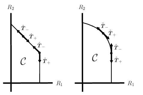
be the set of input distributions achieving a given point $(R_{1}^{*},R_{2}^{*})$ of the boundary of $\mathcal{C}$. Note that in contrast with the single-user setting [1, 3, 2], this definition uses an inequality rather than an equality, as one of the mutual information quantities may be strictly larger than the corresponding entry of $\mathbf{R}^{*}$ and yet be first-order optimal. For example, assuming that the capacity region on the left of Figure 1 is achieved by a single input distribution, all points $(R_{1}^{*},R_{2}^{*})$ on the vertical boundary satisfy $I_{12}(P_{X_{1}X_{2}})>R_{1}^{*}+R_{2}^{*}$.

The preceding definitions are analogous to those appearing in previous works such as [4], while the remaining definitions are somewhat less standard. Given the boundary point $(R_{1}^{*},R_{2}^{*})$, we let $\hat{\mathbf{T}}_{-}:=\hat{\mathbf{T}}_{-}(R_{1}^{*},R_{2}^{*})$ and $\hat{\mathbf{T}}_{+}:=\hat{\mathbf{T}}_{+}(R_{1}^{*},R_{2}^{*})$ denote the left and right unit tangent vectors along the boundary of $\mathcal{C}$ in $(R_{1},R_{2})$ space; see Figure 1 for an illustration. Furthermore, we define

$\displaystyle{\mathbf{T}}_{-}:=\begin{bmatrix}\hat{T}_{-,1}\\ \hat{T}_{-,1}+\hat{T}_{-,2}\end{bmatrix},\quad{\mathbf{T}}_{+}:=\begin{bmatrix}\hat{T}_{+,1}\\ \hat{T}_{+,1}+\hat{T}_{+,2}\end{bmatrix}.$

(16)

It is understood that $\hat{\mathbf{T}}_{-}$ and ${\mathbf{T}}_{-}$ (respectively, $\hat{\mathbf{T}}_{+}$ and ${\mathbf{T}}_{+}$) are undefined when $R_{1}^{*}=0$ (respectively, $R_{2}^{*}=0$). As is observed in Figure 1, we have $\hat{\mathbf{T}}_{-}=-\hat{\mathbf{T}}_{+}$ on the curved and straight-line parts of $\mathcal{C}$, and $\hat{\mathbf{T}}_{-}\neq-\hat{\mathbf{T}}_{+}$ when there is a sudden change in slope (e.g. at a corner point).

The following set of vectors can be thought of as those that point strictly inside $\mathcal{C}$ when placed at $(R_{1}^{*},R_{2}^{*})$:

$$\hat{\mathcal{V}}(R_{1}^{*},R_{2}^{*}):=\\ \big\{\mathbf{v}\in\mathbb{R}^{2}\,:\,(R_{1}^{*},R_{2}^{*})+\alpha\mathbf{v}\in\mathcal{C}\text{ for some }\alpha>0\big\}.$$

(17)

Using this definition, we set

$\displaystyle\mathcal{V}(R_{1}^{*},R_{2}^{*}):=\mathrm{cl}\bigg(\bigcup_{(v_{1},v_{2})\in\hat{\mathcal{V}}(R_{1}^{*},R_{2}^{*})}\big\{(v_{1},v_{1}+v_{2})\big\}\bigg).$

(18)

Due to the closure operation, it is readily verified that ${\mathbf{T}}_{-}\in\mathcal{V}$ and ${\mathbf{T}}_{+}\in\mathcal{V}$.

For a given boundary point $(R_{1}^{*},R_{2}^{*})$ and input distribution $P_{X_{1}X_{2}}\in\Pi(R_{1}^{*},R_{2}^{*})$, we define the set $\mathcal{L}_{0}(\varepsilon;R_{1}^{*},R_{2}^{*},P_{X_{1}X_{2}})$ separately for the following three cases:

(i) If $R_{1}^{*}=I_{1}(P_{X_{1}X_{2}})$ and $R_{1}^{*}+R_{2}^{*}<I_{12}(P_{X_{1}X_{2}})$, then

$\displaystyle\mathcal{L}_{0}=\Big\{(L_{1},L_{2})\,:\,L_{1}\leq\sqrt{V_{1}(P_{X_{1}X_{2}})}\Phi^{-1}(\varepsilon)\Big\}$

(19)

(ii) If $R_{1}^{*}<I_{1}(P_{X_{1}X_{2}})$ and $R_{1}^{*}+R_{2}^{*}=I_{12}(P_{X_{1}X_{2}})$, then

$\displaystyle\hskip-0.43057pt\mathcal{L}_{0}=\Big\{(L_{1},L_{2})\,:\,L_{1}+L_{2}\leq\sqrt{V_{12}(P_{X_{1}X_{2}})}\Phi^{-1}(\varepsilon)\Big\}$

(20)

(iii) If $R_{1}^{*}=I_{1}(P_{X_{1}X_{2}})$ and $R_{1}^{*}+R_{2}^{*}=I_{12}(P_{X_{1}X_{2}})$, then

	$\displaystyle\mathcal{L}_{0}=\Big\{(L_{1},L_{2})\,:\,\mathbf{L}\in\bigcup_{\beta\geq 0}\big\{\beta{\mathbf{T}}_{-}+\Psi^{-1}(\mathbf{V}(P_{X_{1}X_{2}}),\varepsilon)\big\}\Big\}$
	$\displaystyle\cup~\Big\{(L_{1},L_{2})\,:\,\mathbf{L}\in\bigcup_{\beta\geq 0}\big\{\beta{\mathbf{T}}_{+}+\Psi^{-1}(\mathbf{V}(P_{X_{1}X_{2}}),\varepsilon)\big\}\Big\}$	,		(21)

where the first (respectively, second) set in the union is understood to be empty when $R_{1}^{*}=0$ (respectively, $R_{2}^{*}=0$).

We are now in a position to state our main result.

Suppose that $\mathcal{X}_{1}=\emptyset$ and $(R_{1}^{*},R_{2}^{*})=(0,C)$, where $C:=\max_{P_{X_{2}}}I(P_{X_{2}},W)$ and $W:\mathcal{X}_{2}\to\mathcal{Y}$. Clearly $L_{1}$ plays no role, and Theorem 1 states that the achievable values of $L_{2}$ are precisely those in the set

$$\mathcal{L}_{2}(\varepsilon):=\bigcup_{P_{X_{2}}\in\Pi}\Big\{L_{2}:L_{2}\leq\sqrt{V(P_{X_{2}})}\Phi^{-1}(\varepsilon)\Big\},$$

(23)

where $\Pi:=\{P_{X_{2}}:I(P_{X_{2}},W)=C\}$, and $V(\cdot):=V_{12}(\cdot)$ is the conditional information variance [3]. Letting $L^{*}:=\sup\mathcal{L}_{2}(\varepsilon)$ be the second-order coding rate [2] of the discrete memoryless channel (DMC) $W:\mathcal{X}_{2}\to\mathcal{Y}$, we readily obtain

$$L^{*}=\left\{\begin{array}[]{cc}\sqrt{\min_{P_{X_{2}}\in\Pi}V(P_{X_{2}})}\,\Phi^{-1}(\varepsilon)&\varepsilon<\frac{1}{2}\\ \sqrt{\max_{P_{X_{2}}\in\Pi}V(P_{X_{2}})}\,\Phi^{-1}(\varepsilon)&\varepsilon\geq\frac{1}{2}.\end{array}\right.$$

(24)

Thus, our main result reduces to the classical result of Strassen [1, Thm. 3.1] for the single-user setting (see also [2, 3]). This illustrates the necessity of the set $\Pi(R_{1}^{*},R_{2}^{*})$ in the characterization of $\mathcal{L}(\varepsilon;R_{1}^{*},R_{2}^{*})$ in Theorem 1. Such a set is not needed in the Gaussian setting [7], as every boundary point is achieved uniquely by a single multivariate Gaussian distribution. Another notable difference in Theorem 1 compared to [7] is the use of left and right tangent vectors instead of a single derivative vector.

Both of the preceding differences were also recently observed in an achievability result for the standard MAC [10]. However, no converse results were given in [10], and the main novelty of the present paper is in the converse proof.

It is not difficult to show that $\mathcal{L}$ equals a half-space whenever $\hat{\mathbf{T}}_{-}=-\hat{\mathbf{T}}_{+}$, as was observed in [7, 10]. A less obvious fact is that the unions over $\beta$ in (21) can be replaced by $\beta=0$ whenever the corresponding input distribution $P_{X_{1}X_{2}}$ achieves all of the boundary points in a neighborhood of $(R_{1}^{*},R_{2}^{*})$. We refer the reader to [7, 10] for further discussions and illustrative numerical examples.

The achievability part of Theorem 1 is proved using a similar (yet simpler) argument to that of the standard MAC given in [10], so we only provide a brief outline.

We use constant-composition superposition coding with coded time sharing [8, Sec. 4.5.3]. We set $\mathcal{U}:=\{1,2\}$, fix a joint distribution $Q_{UX_{1}X_{2}}$ (to be specified shortly), and let $Q_{UX_{1}X_{2},n}$ be the closest corresponding joint type. We write the marginal distributions in the usual way (e.g. $Q_{X_{1}|U,n}$). We let $\mathbf{u}$ be a deterministic time-sharing sequence with $nQ_{U,n}(1)$ ones and $nQ_{U,n}(2)$ twos. We first generate the $M_{2,n}$ codewords of user 2 independently according to the uniform distribution on $T_{\mathbf{u}}^{n}(Q_{X_{1}|U,n})$. For each $m_{2}$, we generate $M_{1,n}$ codewords for user 1 conditionally independently according to the uniform distribution on $T_{\mathbf{u}\mathbf{x}_{2}}^{n}(Q_{X_{1}|X_{2}U,n})$, where $\mathbf{x}_{2}$ is the codeword for user 2 corresponding to $m_{2}$.

We fix $\beta\geq 0$ and choose $Q_{UX_{1}X_{2}}$ such that $Q_{U}(1)=1-\frac{\beta}{\sqrt{n}}$ and $Q_{U}(2)=\frac{\beta}{\sqrt{n}}$, let $Q_{X_{1}X_{2}|U=1}$ be an input distribution $P_{X_{1}X_{2}}$ achieving the boundary point of interest, and let $Q_{X_{1}X_{2}|U=2}$ be an input distribution $P^{\prime}_{X_{1}X_{2}}$ achieving a different boundary point. We define the shorthands $\mathbf{I}:=\mathbf{I}(P_{X_{1}X_{2}})$, $\mathbf{V}:=\mathbf{V}(P_{X_{1}X_{2}})$ and $\mathbf{I}^{\prime}:=\mathbf{I}(P^{\prime}_{X_{1}X_{2}})$. Using the generalized Feinstein bound given in [7] along with the multivariate Berry-Esseen theorem, we can use the arguments of [10] to conclude that all rate pairs $(R_{1,n},R_{2,n})$ satisfying

$$\mathbf{R}_{n}\in\mathbf{I}+\frac{1}{\sqrt{n}}\Big(\beta(\mathbf{I}^{\prime}-\mathbf{I})+\Psi^{-1}(\mathbf{V},\varepsilon)\Big)+g(n)\mathbf{1}$$

(25)

are $(n,\varepsilon)$-achievable for some $g(n)=O\big(n^{1/4}\big)$ depending on $\varepsilon$, $\beta$, $P_{X_{1}X_{2}}$ and $P^{\prime}_{X_{1}X_{2}}$. Note that this argument may require a reduction to a lower dimension for singular dispersion matrices; an analogous reduction will be given in the converse proof below.

The achievability part of Theorem 1 now follows as in [10]. In the cases corresponding to (19)–(20), we eliminate one of the two element-wise inequalities from (25) to obtain the desired result. For the remaining case corresponding to (21), we obtain the first (respectively, second) term in the union by letting $P_{X_{1}X_{2}}^{\prime}$ achieve a boundary point approaching $(R_{1}^{*},R_{2}^{*})$ from the left (respectively, right).

The converse proof builds on that for the Gaussian case [7], but contains more new ideas compared to the achievability part. We thus provide a more detailed treatment.

References

- [1] V. Strassen. Asymptotische Abschätzungen in Shannons Informationstheorie. In Trans. Third Prague Conf. Inf. Theory, pages 689–723, Prague, 1962.
- [2] M. Hayashi. Information spectrum approach to second-order coding rate in channel coding. IEEE Trans. Inf. Th., 55(10):4947–66, 2009.
- [3] Y. Polyanskiy, H. V. Poor, and S. Verdú. Channel coding rate in the finite blocklength regime. IEEE Trans. Inf. Th., 56(5):2307–59, 2010.
- [4] V. Y. F. Tan and O. Kosut. On the dispersions of three network information theory problems. IEEE Trans. Inf. Th., 60(2):881–903, 2014.
- [5] R. Nomura and T. S. Han. Second-order Slepian-Wolf coding theorems for non-mixed and mixed sources. IEEE Trans. Inf. Th., 60(9):5553–5572, 2014.
- [6] S.-Q. Le, V. Y. F. Tan, and M. Motani. Second-order asymptotics for the Gaussian interference channel with strictly very strong interference. In Int. Symp. Inf. Th., Honolulu, HI, July 2014.
- [7] J. Scarlett and V. Y. F. Tan. Second-order asymptotics for the Gaussian MAC with degraded message sets. arXiv:1310.1197 [cs.IT].
- [8] A. El Gamal and Y.-H. Kim. Network Information Theory. Cambridge University Press, Cambridge, U.K., 2012.
- [9] I. Csiszár and J. Körner. Information Theory: Coding Theorems for Discrete Memoryless Systems. Cambridge University Press, 2011.
- [10] J. Scarlett, A. Martinez, and A. Guillén i Fàbregas. Second-order rate region of constant-composition codes for the multiple-access channel. IEEE Trans. Inf. Th., 61(1):157–172, Jan. 2015.