Imfit: A Fast, Flexible New Program for Astronomical Image Fitting
Abstract
I describe a new, open-source astronomical image-fitting program called imfit, specialized for galaxies but potentially useful for other sources, which is fast, flexible, and highly extensible. A key characteristic of the program is an object-oriented design which allows new types of image components (2D surface-brightness functions) to be easily written and added to the program. Image functions provided with imfit include the usual suspects for galaxy decompositions (Sérsic, exponential, Gaussian), along with Core-Sérsic and broken-exponential profiles, elliptical rings, and three components which perform line-of-sight integration through 3D luminosity-density models of disks and rings seen at arbitrary inclinations.
Available minimization algorithms include Levenberg-Marquardt, Nelder-Mead simplex, and Differential Evolution, allowing trade-offs between speed and decreased sensitivity to local minima in the fit landscape. Minimization can be done using the standard statistic (using either data or model values to estimate per-pixel Gaussian errors, or else user-supplied error images) or Poisson-based maximum-likelihood statistics; the latter approach is particularly appropriate for cases of Poisson data in the low-count regime. I show that fitting low-S/N galaxy images using minimization and individual-pixel Gaussian uncertainties can lead to significant biases in fitted parameter values, which are avoided if a Poisson-based statistic is used; this is true even when Gaussian read noise is present.
Subject headings
methods: data analysis — techniques: image processing — techniques: photometric — galaxies: structure — galaxies: bulges — galaxies: photometryI. Introduction
Galaxies are morphologically complex entities. Even seemingly simple systems like elliptical galaxies can have outer envelopes and distinct cores or nuclei, while so-called “bulge-less” spiral galaxies can still have nuclear star clusters and disks with complex radial or vertical profiles. In order to accurately describe the structure of galaxies, it is often necessary to decompose galaxies into component substructures. Even single-component systems are often modeled with analytic functions in order to derive quantitative measurements such as scale lengths or half-light radii, Sérsic indices, etc.
The traditional method for dealing with this complexity has been to model 1D surface-brightness profiles of galaxies – derived from 2D images – as the sum of separate, additive components (e.g., bulge + disk); pioneering examples of this include work by Kormendy [42], Burstein [7], Tsikoudi [81], Tsikoudi [82], Boroson [3], Send [70], and Hickson et al. [39]. While this 1D approach can be conceptually and computationally simple, it has a number of limitations, above and beyond the fact that it involves discarding most of the data contained in an image. To begin with, there are uncertainties about what type of 1D profile to use – should one use major-axis cuts or profiles from ellipse fits to isophotes, should the independent variable be semi-major axis or mean radius, etc. It is also difficult to correctly account for the effects of image resolution when fitting 1D profiles; attempts to do so generally require simple analytic models of the point-spread function (PSF), extensive numerical integrations, and the assumption of circular symmetry for the PSF, the surface-brightness function, or both [64, 67, 79, 66, e.g.,]. Furthermore, there are often intrinsic degeneracies involved: images of galaxies with non-axisymmetric components such as bars can yield 1D profiles resembling those from galaxies with axisymmetric bulges, which makes for considerable ambiguity in interpretation. Finally, if one is interested in the properties of non-axisymmetric components (bars, elliptical rings, spiral arms) themselves, it is generally impossible to extract these from 1D profiles.
A better approach in many cases is to directly fit the images with 2D surface-brightness models. Early approaches along this line include those of Capaccioli et al. [9], Shaw & Gilmore [72], and Scorza & Bender [69]. The first general, self-consistent 2D bulge+disk modeling of galaxy images – that is, constructing a full 2D model image, comparing its intensity values with the observed image pixel-by-pixel, and iteratively updating the parameters until the is minimized – was that of Byun & Freeman [8], with de Jong [18] being the first to include extra, non-axisymmetric components (bars) in fitting galaxy images. An interesting alternate approach developed at roughly the same time was the Multi-Gaussian Expansion method [52, 25, 10], which involves modeling both PSF and image as the sum of an arbitrary number of elliptical Gaussians; the drawback is the difficulty that lies in trying to associate sets of Gaussians with particular structural components and parameters.
The most commonly used galaxy-fitting codes at the present time are probably gim2d [74, 75],11 1 https://www.astrosci.ca/users/GIM2D/ galfit [59, 60],22 2 http://users.obs.carnegiescience.edu/ peng/work/galfit/galfit.html budda [19, 33],33 3 http://www.sc.eso.org/˜dgadotti/budda.html and MGE [25, 10].44 4 http://www-astro.physics.ox.ac.uk/˜mxc/ software/ gim2d is specialized for bulge-disk decompositions and is implemented as an iraf package, using the Metropolis algorithm to minimize the total for models containing an exponential disk and a Sérsic bulge. budda is written in fortran and is also specialized for bulge-disk decompositions, though it includes a wider variety of possible components: exponential disk (with optional double-exponential profile), Sérsic bulge, Sérsic bar, analytic edge-on disk, and nuclear point source. It uses a version of the Nelder-Mead simplex method [55], also known as the “downhill simplex”, for minimization. galfit, which is written in C, is the most general of these codes, since it allows for arbitrary combinations of components (including components with different centers, which allows the simultaneous fitting of overlapping galaxies) and includes the largest set of possible components; the latest version [60] includes options for spiral and other parametric modulation of the basic components. galfit uses a version of the fast Levenberg-Marquardt gradient-search method [44, 49] for its minimization. MGE, available in IDL and Python versions, is rather different from the other codes in that it uses what is effectively a non-parametric approach, fitting images using the sum of an arbitrary number of elliptical Gaussians (it is similar to galfit in using the Levenberg-Marquardt method for minimization during the fitting process.)
For most astronomical image-fitting programs the source code is not generally available, or else is encumbered by non–open-source licenses. Even when the code is available, it is not easy to extend the built-in sets of predefined image components. The simplest codes provide only elliptical components with exponential and Sérsic surface brightness profiles; more sophisticated codes such as budda and (especially) galfit provide a larger set of components, including some sophisticated ways of perturbing the components in the case of galfit. But if one wants to add completely new functions, this is not easy. (The case of MGE is somewhat different, since it does not allow parametric functions at all.)
As an example of why one might want to do this, consider the case of edge-on (or nearly edge-on) disk galaxies. Both budda and galfit include versions of the analytical solution for a perfectly edge-on, axisymmetric, radial-exponential disk of van der Kruit & Searle [85], with a function for the vertical light distribution. But real galaxy disks are not always perfectly edge-on, do not all have single-exponential radial structures, and their vertical structure may in some cases be better described by a sech or exponential profile, or something in between [84, 17, 61, 91, e.g.,]. Various authors studying edge-on disks have suggested that models using radial profiles other than a pure exponential would be best fit via line-of-sight integration through 3D luminosity-density models [85, 62, 61, e.g.,]. More sophisticated approaches could even involve line-of-sight integrations that account for scattering and absorption by dust [90, 88, 89, e.g.,].
Another potential disadvantage of existing codes is that they rely on the Gaussian approximation of Poisson statistics for the fitting process. While this is eminently sensible for dealing with many CCD and near-IR images, it can in some cases produce biases when applied to images with low count rates (see Humphrey et al. 41 and Section IX of this paper). This is why packages for fitting X-ray data, such as sherpa [30], often include alternate statistics for fits.
In this paper, I present imfit, a new, open-source image-fitting code designed to overcome some of the limitations mentioned above. In particular, imfit uses an object-oriented design which makes it relatively easy to add new, user-designed image components; it also provides multiple fitting algorithms and statistical approaches. It can also be extremely fast, since it is able to take advantage of multiple CPU cores on the same machine to execute calculations in parallel.
The outline of this paper is as follows. Section II provides a quick sketch of how the program works, while Section III details the process of generating model images and the configuration files which describe the models. The different underlying statistical models and minimization algorithms used in the fitting process are covered in Section IV; methods for estimating confidence intervals for fitted parameters are discussed in Section V. The default 2D image functions which can be used in models are presented in Section VI; this includes functions which perform line-of-sight integration through 3D luminosity-density models (Section VI.2). After a brief discussion of coding details (Section VII), two examples of using imfit to model galaxy images are presented in Section VIII: the first involves fitting a moderately-inclined spiral galaxy with disk, bar, and ring components, while the second fits an edge-on spiral galaxy with thin and thick edge-on disk components. Finally, Section IX discusses possible biases to fitted parameters when the standard statistic is used in the presence of low-count images, using both model images and real images of elliptical galaxies. An Appendix discusses the relative sizes and accuracies of parameter error estimates using the two methods available in imfit.
To avoid any confusion, I note that the program described in this paper is unrelated to tasks with the same name and somewhat similar (if limited) functionality in pre-existing astronomical software, such as the “imfit” tasks in the radio-astronomy packages aips and miriad and the “images.imfit” package in iraf.
II. General Outline of the Program
Imfit begins by processing command-line options and then reads in the data image, along with any optional, user-specified PSF, noise, and mask images (all in fits format). The configuration file is also read; this specifies the model which will be fit to the data image, including initial parameter values and parameter limits, if any (see Section III.1).
The program then creates an instance of the ModelObject class, which holds the relevant data structures, instances of the image functions specified by the configuration file, and the general code necessary for computing a model image. If minimization (the default) is being done, a noise image is constructed, either from a user-specified fits file already read in or by internally generating one, assuming the Gaussian approximation for Poisson noise. The noise image is then converted to form and combined with the mask image, if any, to form a final weight image used for calculating the value. (If model-based minimization has been specified, then the noise image, which is based on the model image, is recalculated and combined with the mask image every time a new model image is computed; if a Poisson maximum-likelihood statistic ( or PMLR; see Section IV.1.3) is being used for minimization, then no noise image is read or created and the weight image is constructed directly from the mask image. See Section IV.1 for more on the different statistical approaches.)
The actual fitting process is overseen by one of three possible nonlinear minimization algorithms, as specified by the user. These algorithms proceed by generating or modifying a set of parameter values and feeding these values to the aforementioned model object, which in turn calculates the corresponding model image, convolves it with the PSF (if PSF convolution is part of the model), and then calculates the fit statistic (e.g., ) by comparing the model image with the stored data image. The resulting fit statistic is returned to the minimization algorithm, which then updates the parameter values and repeats the process according to the details of the particular method, until the necessary stop criterion is reached – e.g., no further significant reduction in the fit statistic, or a maximum number of iterations. Finally, a summary of the fit results is printed to the screen and saved to a file, along with any additional user-requested outputs (final model image, final residual image, etc.).
III. Constructing the Model Image
III.1. Configuration File
The model which will be fit to the data image is specified by a configuration file, which is a text file with a relatively simple and easy-to-read format; see Figure 1 for an example.
The basic format for this file is a set of one or more “function blocks”, each of which contains a shared center (pixel coordinates) and one or more image functions. A function block can, for example, represent a single galaxy or other astronomical object, which itself has several individual components (e.g., bulge, disk, bar, ring, nucleus, etc.) specified by the individual image functions. Thus, for a basic bulge/disk decomposition the user could create a function block consisting of a single Sérsic function and a single Exponential function. There is, however, no a priori association of any particular image function or functions with any particular galaxy component, nor is there any requirement that a single object must consist of only one function block. The final model is the sum of the contributions from all the individual functions in the configuration file. The number of image functions per function block is unlimited, and the number of function blocks per model is also unlimited.
Each image function is listed by name (e.g., “FUNCTION Sersic’’), followed by the list of its parameters. For each parameter, the user supplies an initial guess for the value, and (optionally) either a comma-separated, two-element list of lower and upper bounds for that parameter or the keyword ‘‘fixed’’ (indicating that the parameter will remain constant during the fit).55 5 Parameter bounds can be used with any of the minimization algorithms; with the Differential Evolution algorithm, they are actually required, though in that case the initial values are ignored; see Section IV.3.
The total set of all individual image-function parameters, along with the central coordinates for each function block, constitutes the parameter vector for the minimization process.
III.2. Image Functions
An image function can be thought of as a black box which accepts a set of parameter values for its general setup, and then accepts individual pixel coordinates and returns a corresponding computed intensity (i.e., surface brightness) value for that pixel. The total intensity for a given pixel in the model image (prior to any PSF convolution) is the sum of the individual values from each image function.
This design means that the main program needs to know nothing about the individual image functions except the number of parameters they take, and which subset of the total parameter vector corresponds to a given image function. The actual calculations carried out by an image function can be as simple or as complex as the user requires, ranging from returning a constant value for each pixel (e.g., the FlatSky function) to performing line-of-sight integration through a 3D luminosity density model (e.g., the ExponentialDisk3D function); user-written image functions could even perform modest simulations in the setup stage.66 6 One should bear in mind that even relatively simple fits will typically require dozens to hundreds of function evaluations during the minimization process, so complex simulations will mean a lengthy fitting process.
The list of currently available image functions, along with descriptions for each, is given in Section VI.
III.3. PSF Convolution
To simulate the effects of atmospheric seeing and telescope optics, model images can be convolved with a PSF image. The latter can be any fits file which contains the point spread function. PSF images should ideally be square with sides measuring an odd number of pixels, with the peak of the PSF centered in the central pixel of the image. (Off-center PSFs can be used, but the resulting convolved model images will of course be shifted.) Imfit automatically normalizes the PSF image when it is read in.
The actual convolution follows the standard approach of using Fast Fourier Transforms of the internally-generated model image and the PSF image, multiplied together, with the output convolved model image being the inverse transform of the product image. The transforms are done with the FFTW library [31, “Fastest Fourier Transform in the West”,],77 7 http://www.fftw.org which has the advantage of being able to perform transforms on images of arbitrary size (i.e., not just images with power-of-two sizes); in addition, it is well-tested and fast, and can use multiple threads to take advantage of multiple processor cores.
To avoid possible edge effects in the convolution, the internal model-image array is expanded on all four sides by the width and height of the PSF image, and all calculations prior to the convolution phase use this full (expanded) image. (For example, given a -pixel data image and a -pixel PSF image, the internal model image would be pixels in size.) This ensures that model pixels corresponding to the edge of the data image are the result of convolution with an extension of the model, rather than with zero-valued pixels or the opposite side of the model image. This is in addition to the zero-padding applied to the top and right-hand sides of the model image during the convolution phase. (I.e., the example -pixel expanded model image would be zero-padded to pixels before computing its Fourier transform, to match with the zero-padded PSF image of the same size.)
III.4. Makeimage: Generating Model Images Without Fitting
A companion program called makeimage is included in the imfit package, built from the same codebase as imfit itself. This program implements the complete model-image construction process, including PSF convolution, and then simply saves the resulting model image as a fits file. It can optionally save separate images, one for each of the individual image functions that make up the model. Since it uses the same configuration-file format as imfit, it can use the output best-fit parameter file that imfit produces (or even an input imfit configuration file).
It also has an optional mode which estimates the fractional flux contributions of the individual components in the model, by summing up the total flux of the individual components on a pixel-by-pixel basis using a very large internal image (by default, pixels). Although analytic expressions for total flux exist for some common components, this is not true for all components – and one of the goals of imfit is to allow users to create and use new image functions without worrying about whether they have simple analytic expressions for the total flux. This mode can be used to help determine such things as bulge/total and other ratios after a fit is found, although it is up to the user to decide which of the components is the “bulge”, which is the “disk”, and so forth.
IV. The Fitting Process
IV.1. The Statistical Background and Options
Given a vector of parameter values , a model image is generated with per-pixel predicted data values , which are then compared with the observed per-pixel data values . The goal is to find the which produces the best match between and , subject to the constraints of the underlying statistical model.
The usual approach is based on the maximum-likelihood principle (which can be derived from a Bayesian perspective if, e.g., one assumes constant priors for the parameter values), and is conventionally known as maximum-likelihood estimation [58, MLE; e.g.,]. To start, one considers the per-pixel likelihood , which is the probability of observing given the model prediction and the underlying statistical model for how the data are generated.
The goal then becomes finding the set of model parameters which maximizes the total likelihood , which is simply the product over all pixels of the individual per-pixel likelihoods:
| (1) |
It is often easier to work with the logarithm of the total likelihood, since this converts a product over pixels into a sum over pixels, and can also simplify the individual per-pixel terms. As most nonlinear optimization algorithms are designed to minimize their objective function, one can use the negative of the log-likelihood. Thus, the goal of the fitting process becomes minimization of the following:
| (2) |
During the actual minimization process, this can often be further simplified by dropping any additive terms in which do not depend on the model, since these are unaffected by changes in the model parameters and are thus irrelevant to the minimization.
In some circumstances, multiplying the negative log-likelihood by 2 produces a value which has the property of being distributed like the distribution [e.g., 11, and references therein]; thus, it is conventional to treat as the statistic to be minimized.
IV.1.1 The (Impractical) General Case: Poisson + Gaussian Statistics
The data in astronomical images typically consist of detections of individual photons from the sky + telescope system (including photons from the source, the sky background, and possibly thermal backgrounds in the telescope) in individual pixels, combined with possible sources of noise due to readout electronics, digitization, etc.
Photon-counting statistics obey the Poisson distribution, where the probability of detecting photons per integration, given a true rate of , is
| (3) |
Additional sources of (additive) noise such as read noise tend to follow Gaussian statistics with a mean of 0 and a dispersion of , so that the probability of measuring counts after the readout process, given an input of counts from the Poisson process, is
| (4) |
The general case for most astronomical images thus involves both Poisson statistics (for photon counts) and Gaussian statistics (for read noise and other sources of additive noise). Unfortunately, even though the individual elements are quite simple, the combination of a Gaussian process acting on the output of a Poisson process leads to the following rather frightening per-pixel likelihood [46, 57, e.g.,]:
| (5) |
The resulting negative log-likelihood for the total image (dropping terms which do not depend on the model) is
| (6) |
Since this still contains an infinite series of exponential and factorial terms, it is clearly rather impractical for fitting images rapidly.
IV.1.2 The Simple Default: Pure Gaussian Statistics
Fortunately, there is a way out which is often (though not always) appropriate astronomical images. This is to use the fact that the Poisson distribution approaches a Gaussian distribution when the counts become large. In this approximation the Poisson distribution is replaced by a Gaussian with . It is customary to assume this is valid when the counts are per pixel [11, e.g.,], though Humphrey et al. [41] point out that biases in the fitted parameters can be present even when counts are higher than this; see Section IX for examples in the case of 2D fits.
Since the contribution from read noise is also nominally Gaussian, the two can be added in quadrature, so that the per-pixel likelihood function is just
| (7) |
where , with being the dispersion of the read-noise term. Twice the negative log-likelihood of the total problem then becomes (dropping terms which do not depend on the model) the familiar sum:
| (8) |
This is the default approach used by imfit: minimizing the as defined in Eqn. 8.
The approximation of the Poisson contribution to is based on the model intensity . Traditionally, it is quite common to estimate this from the data instead, so that . This has the nominal advantage of only needing to be calculated once, at the start of the minimization process, rather than having to be recalculated every time the model is updated.88 8 In practice, the time spent by imfit is dominated by the per-pixel model calculations, so any extra time spent re-estimating the per-pixel values is often negligible. However, the bias resulting from using data-based errors in the low-count regime can be worse than the bias introduced by using model-based values (see Section IX). Both approaches are available in imfit, with data-based estimation being the default. The data-based and model-based approaches are often referred to as “Neyman’s ” and “Pearson’s ”, respectively; in this paper I use the symbols and to distinguish between them.
In the case of “error” images generated by a data-processing pipeline, the corresponding or (variance) values can easily be used in Equation 8 directly, under the assumption that the final per-pixel error distributions are still Gaussian.
IV.1.3 The Simple Alternative: Pure Poisson Statistics
So why not always use the Gaussian approximation, as is done in most image-fitting packages?
In the absence of any noise terms except Poisson statistics – something often true of high-energy detectors, such as X-ray imagers – the individual-pixel likelihoods are just the probabilities of a Poisson process with mean , where the probability of recording counts is
| (9) |
This leads to a very simple version of the negative log-likelihood, often referred to as the “Cash statistic” , after its derivation in Cash [11]:
| (10) |
where the factorial term has been dropped because it does not depend on the model.
A useful alternative is to construct a statistic from the likelihood ratio test – that is, a maximum likelihood ratio (MLR) statistic – which is the ratio of the likelihood to the maximum possible likelihood for a given dataset. In the case of Poisson likelihood, the latter is the likelihood when the model values are exactly equal to the data values [37, e.g.,], and so the likelihood ratio is
| (11) |
and the negative log-likelihood version (henceforth PMLR) is
| (12) |
(This is the same as the “CSTAT” statistic available in the sherpa X-ray analysis package and the “Poisson likelihood ratio” described by Dolphin 21.) Comparison with Equation 10 shows that PMLR is identical to apart from terms which depend on the data only and thus do not affect the minimization. In the remainder of this paper, I will refer to and PMLR collectively as Poisson MLE statistics.
Since minimizing PMLR will produce the same best-fitting parameters as minimizing , one might very well wonder what is the point in introducing PMLR. There are two practical advantages in using it. The first is that in the limit of large , statistics such as PMLR approach a distribution and can thus be used as goodness-of-fit indicators [87, 86]. The second is that they are always (since itself is by construction always ); this means they can be used with fast least-squares minimization algorithms. This is the practical drawback to minimizing : unlike PMLR, it can often have negative values, and thus requires one of the slower minimization algorithms.
Humphrey et al. [41] point out that using a Poisson MLE statistic (e.g., ) is preferable to using or even when the counts are above the nominal limit of per pixel, since fitting pure-Poisson data using the or Gaussian approximations can lead to biases in the derived model parameters. Section IX presents some examples of this effect using both artificial and real galaxy images, and shows that the effect persists even when moderate (Gaussian) read noise is also present.
Using a Poisson MLE statistic such as or PMLR is also appropriate when fitting simulated images, such as those made from projections of -body models, as long as the units are particles per pixel or something similar.
For convenience, Table 1 summarizes the main symbols and terms from this section which are used elsewhere in the paper.
| Term | Explanation |
|---|---|
| Poisson MLE | Maximum-likelihood estimation based on Poisson statistics |
| (includes both and PMLR) | |
| Poisson MLE statistic from Cash [11] | |
| PMLR | Poisson MLE statistic from maximum likelihood ratio |
| Gaussian MLE statistic using data pixel values for | |
| (“Neyman’s ”) | |
| Gaussian MLE statistic using model pixel values for | |
| (“Pearson’s ”) |
IV.2. Implementation: Specifying Per-Pixel Errors and Masking
Imfit’s default behavior, as mentioned above, is to use as the statistic for minimization. To do so, the individual, per-pixel Gaussian errors must be available. If a separate error or noise map is not supplied by the user (see below), imfit estimates values from either the data values or the model values, using the Gaussian approximation to Poisson statistics. To ensure this estimate is as accurate as possible, the data or model values must at some point be converted from counts to actual detected photons (e.g., photoelectrons), and any previously subtracted background must be accounted for.
By default, imfit estimates the values from the data image by including the effects of A/D gain, prior subtraction of a (constant) background, and read noise. Rather than converting the image to electrons pixel-1 and then estimating the values, imfit generates values in the same units as the input image:
| (13) |
where is the data intensity in counts pixel-1, is any pre-subtracted sky background in the same units, is the read noise in electrons, is the number of separate images combined (averaged or median) to form the data image, and is the “effective gain” (the product of the gain, , and optionally the exposure time if the image pixel values are actually in units of counts s-1 pixel-1 rather than integrated counts pixel-1). If model-based minimization is used, then model intensity values are used in place of in Equation 13. In this case, the values must be recomputed each time a new model image is generated, though in practice this adds very little time to the overall fitting process.
If a mask image has been supplied, it is converted internally so that its pixels have values for valid pixels and for bad pixels. Then the mask values are divided by the variances to form a weight-map image, where individual pixels have values of . These weights are then used for the actual calculation:
| (14) |
Instead of data-based or model-based errors, the user can also supply an error or noise map in the form of a fits image, such as might be produced by a reduction pipeline. The individual pixel values in this image can be Gaussian errors, variances (), or even pre-computed weight values .
In the case of Cash-statistic minimization, the sum is computed directly based on Equation 10; for PMLR minimization, Equation 12 is used. The “weight map” in either case is then based directly on the mask image, if any (so all pixels in the resulting weight map have values of or 1). The actual minimized quantities are thus
| (15) |
and
| (16) |
with and .
IV.3. Minimization Algorithms
IV.3.1 Levenberg-Marquardt
The default minimization algorithm used by imfit is a robust implementation of the Levenberg-Marquardt (L-M) gradient search method [49], based on the MINPACK-1 version of Moré [53] and modified by Craig Markwardt [48],99 9 http:// purl.com/net/mpfit which includes optional lower and upper bounds on parameter values. This version of the basic L-M algorithm also includes auxiliary code for doing numerical differentiation of the objective function, and thus the various image functions do not need to provide their own derivatives, which considerably simplifies things when it comes to writing new functions.
The L-M algorithm has the key advantage of being very fast, which is a useful quality when one is fitting large images with a complex set of functions and PSF convolution. It has the minor disadvantage of requiring an initial starting guess for the parameter values, and it has two more significant disadvantages. The first is that like gradient-search methods in general it is prone to becoming trapped in local minima in the objective-function landscape. The second is that it is designed to work with least-squares objective functions, where the objective function values are assumed to be always . In fact, the L-M algorithm makes use of a vector of the individual contributions from each pixel to the total , and these values as well (not just the sum) must be nonnegative. For the case, this is always true; but this is not guaranteed to be true for the Cash statistic . Thus, it would be quite possible for the L-M minimizer to fail to find the best-fitting solution for a particular image, simply because the solution has a value . (Fortunately, minimizing PMLR leads to the same solution as minimizing , and the individual terms of PMLR are always nonnegative.)
IV.3.2 Nelder-Mead Simplex
A second, more general algorithm available in imfit is the Nelder-Mead simplex method [55], with constraints as suggested by Box [4], implemented in the NLopt library.1010 10 Steven G. Johnson, The NLopt nonlinear-optimization package, http://ab-initio.mit.edu/nlopt. Like the L-M algorithm, this method requires an initial guess for the parameter set; it also includes optional parameter limits. Unlike the L-M algorithm, it works only with the final objective function value and does not assume that this value must be nonnegative; thus, it is suitable for minimizing all the fit statistics used by imfit. It is also as a rule less likely to be caught in local minima than the L-M algorithm. The disadvantage is that it is considerably slower than the L-M method – roughly an order of magnitude so.
IV.3.3 Differential Evolution
A third alternative provided by imfit is a genetic-algorithms approach called Differential Evolution [77, DE;]. This searches the objective-function landscape using a population of parameter-value vectors; with each “generation”, the population is updated by mutating and recombining some of the vectors, with new vectors replacing older vectors if they are better-performing. DE is designed to be – in the context of genetic algorithms – fast and robust while keeping the number of adjustable algorithm parameters (e.g., mutation and crossover rates) to a minimum. It is the least likely of the algorithms used by imfit to become trapped in a local minimum in the objective-function landscape: rather than starting from a single initial guess for the parameter vector, it begins with a set of randomly generated initial-parameter values, sampled from the full range of allowed parameter values; in addition, the crossover-with-mutation used to generate new parameter vectors for successive generations helps the algorithm avoid local minima traps. Thus, in contrast to the other algorithms, it does not require any initial guesses for the parameter values, but does require lower and upper limits for all parameters. It is definitely the slowest of the minimization choices: about an order of magnitude slower than the N-M simplex, and thus roughly two orders of magnitude slower than the L-M algorithm.
The current implementation of DE in imfit uses the “DE/rand-to-best/1/bin” internal strategy, which controls how mutation and crossover are done [77], along with a population size of 10 parameter vectors per free parameter. Since the basic DE algorithm has no default stop conditions, imfit halts the minimization when the best-fitting value of the fit statistic has ceased to change by more than a specified tolerance after 30 generations, or when a maximum of 600 generations is reached.
IV.3.4 Comparison and Recommendations
For most purposes, the default L-M method is probably the best algorithm to use, since it is fast enough to make exploratory fitting (varying the set of functions used, applying different parameter limits, etc.) feasible, and also fast enough to make fitting large numbers of individual objects in a reasonable time possible. If the problem is relatively small (modest image size, few image functions) and the user is concerned about possible local minima, then the N-M simplex or even the DE algorithm can be used.
Table 2 provides a general comparison of the different minimization algorithms, including the time taken for each to find the best fit for a very simple case: a -pixel cutout of an SDSS -band image of the galaxy IC 3478, fit with a single Sérsic function and convolved with a -pixel PSF image. For this simple case, the N-M approach takes times as long as the L-M method, and the DE algorithm takes 60 times as long. (All three algorithms converged to the same solution, so there was no disadvantage to using the L-M method in this case.)
| Algorithm | Initial guess | Bounds | Local-minimum | Minimize ? | Speed | Timing |
|---|---|---|---|---|---|---|
| required | required | vulnerability | example | |||
| (1) | (2) | (3) | (4) | (5) | (6) | (7) |
| Levenberg-Marquardt (L-M) | Yes | No | High | No | Fast | 2.2s |
| Nelder-Mead Simplex (N-M) | Yes | No | Medium | Yes | Slow | 9.1s |
| Differential Evolution (DE) | No | Yes | Low | Yes | Very Slow | 2m15s |
Note. — A comparison of the three nonlinear minimization algorithms available in imfit. Column 1: Algorithm name. Column 2: Notes whether an initial guess of parameter values required. Column 3: Notes whether lower and upper bounds on all parameter values are required. Column 4: Vulnerability of the algorithm to becoming trapped in local minima in the (or other objective function) landscape. Column 5: Notes whether algorithm can minimize the Cash statistic in addition to and PMLR. Column 6: General speed. Column 7: Approximate time taken for fitting a pixel SDSS galaxy image (single Sérsic function + PSF convolution), using a MacBook Pro with a quad-core Intel Core i7 2.3 GHz CPU (2011 model).
IV.4. Outputs and “Goodness of Fit” Measures
When imfit finishes, it outputs the parameters of the best fit (along with possible confidence intervals; see Section V) to the screen and to a text file; it also prints the final value of the fit-statistic. The best-fitting model image and the residual (data model) image can optionally be saved to fits files as well.
For fits which minimize , imfit also prints the reduced value, which can be used (with caution) as an indication of the goodness of the fit. (The best-fit value of PMLR can also be converted to a reduced- equivalent with the same properties.) For fits which minimize the Cash statistic, there is no direct equivalent to the reduced ; the actual value of the Cash statistic does not have any directly useful meaning by itself.
All the fit statistics (including ) can also be used to derive comparative measures of how well different models fit the same data. To this end, imfit computes two likelihood-based quantities which can be used to compare different models. The first is the Akaike Information Criterion (AIC, Akaike 1), which is based on an information-theoretic approach. Imfit uses the recommended, bias-corrected version of this statistic:
| (17) |
where is the likelihood value, is the number of (free) parameters in the model and is the number of data points. The second quantity is the Bayesian Information Criterion (BIC, Schwarz 68), which is
| (18) |
When two or more models fit to the same data are compared, the model with the lowest AIC (or BIC) is preferred, though a difference AIC or BIC of at least is usually required before one model can be deemed clearly superior (or inferior); see, e.g., Takeuchi [78] and Liddle [45] for discussions of AIC and BIC in astronomical contexts, and Burnham & Anderson [6] for more general background. Needless to say, all models being compared in this manner should be fit by minimizing the same fit statistic.
V. Confidence Intervals for Fitted Parameters
In addition to its speed, the Levenberg-Marquardt minimization algorithm has the convenient advantage that it can automatically produce a set of approximate, 1- confidence intervals for the fitted parameters as a side product of the minimization process; this comes from inverting the Hessian matrix computed during the minimization process [63, see, e.g., Section 15.5 of].
The other minimization algorithms available in imfit do not compute confidence intervals. Although one can, as a workaround, re-run imfit using the L-M algorithm on a solution that was found using one of the other algorithms, this will not work if (rather than or PMLR) was being minimized (see Section IV.3).
An alternate method of estimating confidence intervals is provided by bootstrap resampling [24]. Each iteration of the resampling process generates a new data image by sampling pixel values, with replacement, from the original data image. (What is actually generated inside imfit is a resampled vector of pixel indices into the image, excluding those indices corresponding to masked pixels; the corresponding coordinates and intensities then form the resampled data.) The fit is then re-run with the best-fit parameters from the original fit as starting values, using the L-M algorithm for and PMLR minimization cases and the N-M simplex algorithm when minimization is being done. After iterations, the combined set of bootstrapped parameter values is used as the distribution of parameter values, from which properly asymmetric 68% confidence intervals are directly determined, along with the standard deviation. (The 68% confidence interval corresponds to - if the distribution is close to Gaussian.)
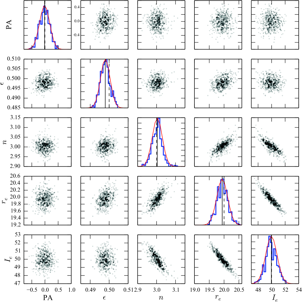
In addition, the full set of best-fit parameters from all the bootstrap iterations can optionally be saved to a file, which potentially allows for more sophisticated analyses. Figure 2 shows a scatter-plot matrix comparing parameter values for five parameters of a simple Sérsic fit to an image of a model Sérsic galaxy with noise (see Section IX for details of the model images). One can see that the distributions are approximately Gaussian, have dispersions similar to those from the L-M estimates (plotted as Gaussians using red curves), and also that certain parameter distributions are correlated (e.g., and or, more weakly, ellipticity and ). Of course, this simple case ignores the complexities and sources of error involved in fitting real images of galaxies; see the Appendix for sample comparisons of L-M and bootstrap error estimates for a small set of real-galaxy images.
The only drawback of the bootstrap-resampling approach is the cost in time. Since bootstrap resampling should ideally use a minimum of several hundred to one thousand or more iterations, one ends up, in effect, re-running the fit that many times. (Some time is saved by starting each fit with the original best-fit parameter values, since those will almost always be close to the best-fit solution for the resampled data.)
VI. Image Functions
Image functions are implemented in imfit as subclasses of an abstract base class called FunctionObject. The rest of the program does not need to know the details of the individual functions, only that they adhere to the FunctionObject interface. This makes it relatively simple to add new image functions to the program: write a header file and an implementation file for the new function, add a reference to it in another source file, and recompile the program. Further notes on how to do this are included in the documentation.
This section describes the various default image functions that come with imfit. Specifications for the actual parameters (e.g., the order that imfit expects to find them in) are included in the documentation, and a summary of all available function names and their corresponding parameter lists can be printed using the --list-parameters command-line flag.
VI.1. 2D Components
Most image functions, unless otherwise noted, have two ‘‘geometric’’ parameters: the position angle PA in degrees counter-clockwise from the vertical axis of the image1111 11 Reproducing the usual convention for images with standard astronomical orientation, where north is up and east is to the left. and the ellipticity , where and are the semi-major and semi-minor axes, respectively.
In most cases, the image function internally converts the ellipticity to an axis ratio () and the position angle to an angle relative to the image -axis (), in radians. Then for each input pixel (or subpixel if pixel subsampling is being done) with image coordinates a scaled radius is computed as
| (19) |
where and are coordinates in the reference frame centered on the image-function center and rotated to its position angle:
| (20) | |||||
This scaled radius is then used to compute the actual intensity, using the appropriate 1-D intensity function (see descriptions of individual image functions, below).
Pure circular versions of any of these functions can be had by specifying that the ellipticity parameter is fixed, with a value of 0. Some functions (e.g., EdgeOnDisk) have only the position angle as a geometric parameter, and instead of computing a scaled radius, convert the pixel coordinates to corresponding and values in the rotated 2D coordinate system of the model function.
VI.1.1 FlatSky
This is a very basic function which produces a uniform background: for all pixels. Unlike most image functions, it has no geometric parameters.
VI.1.2 Gaussian
This is an elliptical 2D Gaussian function, with central surface brightness and dispersion . The intensity profile is given by
| (21) |
VI.1.3 Moffat
This is an elliptical 2D function with a Moffat [51] function for the surface brightness profile, with parameters for the central surface brightness , full-width half-maximum (FWHM), and the shape parameter . The intensity profile is given by
| (22) |
where is defined as
| (23) |
In practice, FWHM describes the overall width of the profile, while describes the strength of the wings: lower values of mean more intensity in the wings than is the case for a Gaussian (as , the Moffat profile converges to a Gaussian).
The Moffat function is often a good approximation to typical telescope PSFs (see, e.g., Trujillo et al. 79), and makeimage can easily be used to generate Moffat PSF images.
VI.1.4 Exponential and Exponential_GenEllipse
The Exponential function is an elliptical 2D exponential function, with parameters for the central surface brightness and the exponential scale length . The intensity profile is given by
| (24) |
together with the position angle and ellipticity, there are a total of four parameters. This is a good default for galaxy disks seen at inclinations , though the majority of disk galaxies have profiles which are more complicated than a simple exponential [36, e.g.,].
The Exponential_GenEllipse function is identical to the Exponential function except for allowing the use of generalized ellipses (with shapes ranging from “disky” to pure elliptical to “boxy”) for the isophote shapes. Following Athanassoula et al. [2] and Peng et al. [59], the shape of the elliptical isophotes is controlled by the parameter, such that a generalized ellipse with ellipticity is described by
| (25) |
where and are distances from the ellipse center in the coordinate system aligned with the ellipse major axis ( corresponds to in the original formulation of Athanassoula et al.). Thus, values of correspond to disky isophotes, while values describe boxy isophotes; for a perfect ellipse.
VI.1.5 Sersic and Sersic_GenEllipse
This pair of related functions is analogous to the Exponential and Exponential_GenEllipse pair above, except that the intensity profile is given by the Sérsic [71] function:
| (26) |
where is the surface brightness at the effective (half-light) radius and is the index controlling the shape of the intensity profile. The value of is formally given by the solution to the transcendental equation
| (27) |
where is the gamma function and is the incomplete gamma function. However, in the current implementation is calculated via the polynomial approximation of Ciotti & Bertin [14] when and the approximation of MacArthur et al. [47] when .
The Sérsic profile is equivalent to the de Vaucouleurs () profile when , to an exponential when , and to a Gaussian when ; it has become the de facto standard for fitting the surface-brightness profiles of elliptical galaxies and bulges. Though the empirical justification for doing so is rather limited, the combination a Sérsic profile with and isophotes with a boxy shape is often used to represent bars when fitting images of disk galaxies. In addition, the combination of boxy isophotes and high values may be appropriate for modeling luminous boxy elliptical galaxies.
VI.1.6 Core-Sersic
This function generates an elliptical 2D function where the major-axis intensity profile is given by the Core-Sérsic model [35, 80], which was designed to fit the profiles of so-called “core” galaxies [29, 65, 22, 23, 66, e.g.,]. It consists of a Sérsic profile (parameterized by and ) for radii the break radius and a single power law with index for radii . The transition between the two regimes is mediated by the dimensionless parameter : for low values of , the transition is very gradual and smooth, while for high values of the transition becomes very abrupt (a perfectly sharp transition can be approximated by setting equal to some large number, such as 100). The intensity profile is given by
| (28) |
where is the same as for the Sérsic function.
The overall intensity scaling is set by , the intensity at the break radius :
| (29) |
VI.1.7 BrokenExponential
This is similar to the Exponential function, but it has two exponential radial zones (with different scalelengths) joined by a transition region at of variable sharpness:
| (30) |
where is the central intensity of the inner exponential, and are the inner and outer exponential scale lengths, is the break radius, and parameterizes the sharpness of the break. Low values of mean very smooth, gradual breaks, while high values correspond to abrupt transitions. is a scaling factor,1212 12 As pointed out by Muñoz-Mateos et al. [54], the original definition of this factor in Eqn. 6 of Erwin et al. [27] contained a typo. given by
| (31) |
see Figure 3 for examples. Note that the parameter has units of length-1 (pixels-1 for the specific case of imfit).
The 1D form of this profile [27] was designed to fit the surface-brightness profiles of disks which are not single-exponential: e.g., disks with truncations or antitruncations [26, 27, 54].
VI.1.8 GaussianRing
This function creates an elliptical ring with a Gaussian radial profile, centered at along the major axis.
| (32) |
See Figure 4 for an example.
VI.1.9 GaussianRing2Side
This function is similar to GaussianRing, except that it uses an asymmetric Gaussian, with different values of for and ). That is, the profile behaves as
| (33) |
for , and
| (34) |
for ; see Figure 4 for an example.
VI.1.10 EdgeOnDisk
This function provides the analytic form for a perfectly edge-on disk with a radial exponential profile, using the Bessel-function solution of van der Kruit & Searle [85] for the radial profile. Although it is common to assume that the vertical profile for galactic disks follows a function, based on the self-gravitating isothermal sheet model of Spitzer [76], van der Kruit [84] suggested a more generalized form for this, one which enables the profile to range from at one extreme to exponential at the other:
| (35) |
with the vertical coordinate and the vertical scale height. The parameter produces a profile when , when , and converges to an exponential as . See de Grijs et al. [17] for examples of fitting the vertical profiles of edge-on galaxy disks using this formula, and Yoachim & Dalcanton [91] for examples of 2D fitting of edge-on galaxy images.
In a coordinate system aligned with the edge-on disk, is the distance from the minor axis (parallel to the major axis) and is the perpendicular direction, with on the major axis. (The latter corresponds to height from the galaxy midplane.) The intensity at is given by
| (36) |
where is the exponential scale length in the disk plane, is the vertical scale height, and is the modified Bessel function of the second kind. The central surface brightness is given by
| (37) |
where is the central luminosity density (see van der Kruit & Searle 85). Note that is the actual input parameter required by the function; is calculated internally.
The result is a function with five parameters: , , , , and the position angle; Figure 5 shows three examples with differing vertical profiles parameterized by , 2, and 100.
VI.1.11 EdgeOnRing
This is a simplistic model for an edge-on ring, using two offset subcomponents located at distance from the center of the function block. Each subcomponent (i.e., each side of the ring) is a 2D Gaussian with central surface brightness and dispersions of in the radial direction and in the vertical direction. It has five parameters: , , , , and the position angle. See Figure 6 for examples of this function.
A potentially more correct (though computationally more expensive) model for a ring seen edge-on ring – or at other inclinations – is provided by the GaussianRing3D function, below.
VI.1.12 EdgeOnRing2Side
This is a slightly more sophisticated variant of EdgeOnRing, where the radial profile for the two components is an asymmetric Gaussian, as in the case of the GaussianRing2Side function, above: the inner () side of each component is a Gaussian with radial dispersion , while the outer side has radial dispersion . It thus has six parameters: , , , , , and the position angle. See the right-hand panel of Figure 6 for an example.
VI.2. 3D Components
All image functions in imfit produce 2D surface-brightness output. However, there is nothing to prevent one from creating a function which does something quite complicated in order to produce this output. As an example, imfit includes three image functions which perform line-of-sight integration through 3D luminosity-density models, in order to produce a 2D projection.
These functions assume a symmetry plane (e.g., the disk plane for a disk galaxy) which is inclined with respect to the line of sight; the inclination is defined as the angle between the line of sight and the normal to the symmetry plane, so that a face-on system has and an edge-on system has . For inclinations , the orientation of the line of nodes (the intersection between the symmetry plane and the sky plane) is specified by a position-angle parameter . Instead of a 2D surface-brightness specification (or 1D radial surface-brightness profile), these functions specify a 3D luminosity density , which is numerically integrated along the line of sight for each pixel of the model image:
| (38) |
To carry out the integration for a pixel located at in the image plane, the coordinates are first transformed to a rotated image plane system centered on the coordinates of the component center , where the line of nodes lies along the axis (cf. Eqn. 20 in Section VI.1):
with being the angle between the line of nodes and the image axis (as in the case of the 2D functions, the actual user-specified parameter is , which is the angle between the line of nodes and the axis).
The line-of-sight coordinate is then defined so that in the sky plane (an instance of the image plane located in 3D space so that it passes through the center of the component), corresponding to
in the component’s native Cartesian coordinate system. A location at along the line of sight then maps into the component coordinate system as
| (39) |
with by construction. The luminosity-density value is then . See Figure 7 for a side-on view of this arrangement.
Although a fully correct integration would run from to , in practice the limit is some large multiple of the component’s normal largest scale size (e.g., 20 times the horizontal disk scale length ), to limit the possibility of numerical integration mishaps.
VI.2.1 ExponentialDisk3D
This function implements a 3D luminosity density model for an axisymmetric disk where the radial profile of the luminosity density is an exponential and the vertical profile follows the function of van der Kruit [84] (see the discussion of the EdgeOnDisk function in Section VI.1.10). The line-of-sight integration is done numerically, using functions from the GNU Scientific Library.
In a cylindrical coordinate system aligned with the disk (where the disk midplane has ), the luminosity density at radius from the central axis and at height from the midplane is given by
| (40) |
where is the exponential scale length in the disk plane, is the vertical scale height, controls the shape of the vertical distribution, and is the central luminosity density. Note that in the context of the introductory discussion above, and .
VI.2.2 BrokenExponentialDisk3D
This function is identical to the ExponentialDisk3D function, except that the radial part of the luminosity density function is given by the broken-exponential profile used by the (2D) BrokenExponential function, above (Section VI.1.7). Thus, the luminosity density at radius from the central axis and at height from the midplane is given by
| (41) |
where is the vertical scale height, and the radial part is given by
| (42) |
with being the central luminosity density and the rest of the parameters as defined for BrokenExponential function (Section VI.1.7).
VI.2.3 GaussianRing3D
This function creates the projection of a 3D elliptical ring, seen at an arbitrary inclination. The ring has a luminosity density with a radial Gaussian profile (centered at along ring’s major axis, with in-plane width ) and a vertical exponential profile (with scale height ). The ring can be imagined as residing in a plane which has its line of nodes at angle and inclination (as for the ExponentialDisk3D function, above); within this plane, the ring’s major axis is at position angle relative to the perpendicular to the line of nodes. To derive the correct luminosity densities for the line-of-sight integration, the component coordinate values from Equation 39 are transformed to a system rotated about the normal to the ring plane, where the ring’s major axis is along the axis:
Figure 9 shows the same GaussianRing3D component (with ellipticity = 0.5) seen at three different inclinations.
VII. Programming Notes
Imfit is written in standard C++, and should be compilable with any modern compiler; it has been tested with GCC versions 4.2 and 4.8 on Mac OS X and GCC version 4.6 on Ubuntu Linux systems. It makes use of several open-source libraries, two which are required (CFITSIO and FFTW) and two which are optional but recommended (NLopt and the GNU Scientific Library). Imfit also uses the Python-based SCons1313 13 http://www.scons.org build system and CxxTest1414 14 http://cxxtest.com for unit tests.
Since the slowest part of the fitting process is almost always computing the model image, imfit is written to take advantage of OpenMP compiler extensions; this allows the computation of the model image to be parceled out into multiple threads, which are then allocated among available processor cores on machines with multiple shared-memory CPUs (including single CPUs with multiple cores). As an example of how effective this can be, tests on a MacBook Pro with a quad-core i7 processor, which has a total of eight virtual threads available, show that basic computation of large images (without PSF convolution) is sped up by a factor of when OpenMP is used. Even when the overhead of an actual fit is included, the total time to fit a four-component model with 21 free parameters (without PSF convolution) to a -pixel image is reduced by a factor of .
Additional computational overhead is imposed when one convolves a model image with a PSF. To mitigate this, imfit uses the FFTW library to compute the necessary Fourier transforms. This is one of the fastest FFT libraries available, and it can be compiled with support for multiple threads. When the same -pixel image fit mentioned above is done including convolution with a -pixel PSF image, the total time drops from s without any multi-threading to s when just the FFT computation is multi-threaded, and down to s when OpenMP threading is enabled as well.
Multithreading can always be reduced or turned off using a command-line option if one does not wish to use all available CPU cores for a given fit.
VIII. Sample Applications
Imfit has been used for several different astronomical applications, including preliminary work on the EUCLID photometric pipeline [43], testing 1D convolution code used in the analysis of core galaxies [66], fitting kinematically decomposed components of the galaxy NGC 7217 [28], determining the PSF for Data Release 2 of the CALIFA survey [34], and separation of bulge and disk components for dynamical modeling of black hole masses in nearby S0 and spiral galaxies (Erwin et al., in prep).
In this section I present two relatively simple examples of using imfit to model images of real galaxies. The first case considers a moderately inclined spiral galaxy with a prominent ring surrounding a bar, where use of a separate ring component considerably improves the fit. The second case is an edge-on disk galaxy with both thin and thick disks; I show how this can be fit using both the analytic pure-edge-on disk component (EdgeOnDisk; Section VI.1.10) and the 3D luminosity-density model of an exponential disk (ExponentialDisk3D; Section VI.2.1).
VIII.1. PGC 35772: Disk, Bar, and Ring
PGC 35772 is a , early/intermediate-type spiral galaxy (classified as SA0/a by de Vaucouleurs et al. 20 and as Sb by Fukugita et al. 32) which was observed as part of the H Galaxy Groups Imaging Survey (HAGGIS; Kulkarni et al., in prep.) using narrow-band filters on the Wide Field Imager of the ESO 2.2m telescope. The upper-left panel of Figure 10 shows the stellar-continuum-filter image (central wavelength nm, slightly blueward of the redshifted H line). Particularly notable is a bright stellar ring, which makes this an interesting test case for including rings in 2D fits of galaxies. Ellipse fits to the image show strong twisting of the isophotal position angle interior to the ring, suggesting a bar is also present.
The rest of Figure 10 shows the results three different fits to the image, each successive fit adding an extra component. These fits use a -pixel cutout of the full WFI image, and were convolved with a Moffat-function image with FWHM = 0.98″, representing the mean PSF (based on Moffat fits to stars in the same image). The best-fit parameters for each model, determined by minimizing PMLR, are listed in Table 3, along with the uncertainties estimated from the L-M covariance matrix. Since the fitting times are short, I also include parameter uncertainties from 500 rounds of bootstrap resampling (in parentheses, following the L-M uncertainties).
The first fit is uses a single Sersic component; the residuals of this fit show a clear excess corresponding to the ring, as well as mis-modeling of the region inside the ring. The fit is improved by switching to an exponential + Sérsic model, with the former component representing the main disk and the latter some combination of the bar + bulge (if any). This two-component model (middle row of the figure) produces less extreme residuals; the best-fitting Sérsic component is elongated and misaligned with the exponential component, so it can be seen to be modeling the bar.
The residuals to this “disk + bar” fit are still significant, however, including the ring itself. To fix this, I include a GaussianRing component (Section VI.1.8) in the third fit (bottom row of Figure 10). The residuals to this fit are better not just in the ring region, but also inside, indicating that this three-component model is doing a much better job of modeling the inner flux of the galaxy (the three-component also has the smallest AIC value of the three models; see Table 3).

| Component | Parameter | Value | units | |
|---|---|---|---|---|
| (1) | (2) | (3) | (4) | (5) |
| Sersic only (AIC ) | ||||
| Sersic | PA | 138.14 | 0.48 (0.34) | deg |
| 0.254 | 0.0038 (0.0024) | |||
| 1.041 | 0.0085 (0.027) | |||
| 39.16 | 0.33 (0.52) | cont. flux | ||
| 8.267 | 0.042 (0.034) | arcsec | ||
| Exponential + Bar (AIC ) | ||||
| Exponential | PA | 137.79 | 0.49 (0.29) | deg |
| (disk) | 0.259 | 0.0039 (0.0021) | ||
| 194.58 | 1.22 (0.97) | cont. flux | ||
| 5.17 | 0.025 (0.014) | arcsec | ||
| Sersic | PA | 16.27 | 3.00 (1.13) | deg |
| (bar) | 0.562 | 0.056 (0.025) | ||
| 0.897 | 0.282 (0.074) | |||
| 171.82 | 25.32 (6.77) | cont. flux | ||
| 0.713 | 0.041 (0.021) | arcsec | ||
| Exponential + Bar + Ring (AIC ) | ||||
| Exponential | PA | 140.70 | 1.25 (0.53) | deg |
| (disk) | 0.277 | 0.0098 (0.0053) | ||
| 111.19 | 11.55 (4.05) | cont. flux | ||
| 5.74 | 0.18 (0.052) | arcsec | ||
| Sersic | PA | 7.27 | 2.28 (1.04) | deg |
| (bar) | 0.364 | 0.028 (0.092) | ||
| 1.14 | 0.114 (0.046) | |||
| 80.78 | 7.25 (2.47) | cont. flux | ||
| 1.42 | 0.080 (0.028) | arcsec | ||
| GaussianRing | PA | 128.40 | 1.69 (0.69) | deg |
| (ring) | 0.258 | 0.013 (0.0053) | ||
| 26.90 | 3.22 (1.10) | cont. flux | ||
| 5.50 | 0.36 (0.14) | arcsec | ||
| 3.43 | 0.22 (0.13) | arcsec | ||
Note. — Results of fitting narrow-band continuum image of spiral galaxy PGC 35771 with progressively more complex models (Sersic; Exponential + Sersic; Exponential + Sersic + GaussianRing). “AIC” = Akaike Information Criterion values for the fits; lower values imply better fits. Column 1: Component used in fit. Column 2: Parameter. Column 3: Best-fit value for parameter. Column 4: Uncertainty on parameter value from L-M covariance matrix; uncertainty from bootstrap resampling is in parentheses. Column 5: Units (“cont. flux” units are erg s-1 cm-2 Å-1 arcsec-2).
VIII.2. IC 5176: Fitting Thin and Thick Disks in an Edge-on Spiral in 2D and 3D
IC 5176 is an edge-on Sbc galaxy, included in a “control” sample of non-boxy-bulge galaxies by Chung & Bureau [12] and Bureau et al. [5]. Chung & Bureau [12] noted that both the gas and stellar kinematics were consistent with an axisymmetric, unbarred disk; Bureau et al. [5] concluded from their -band image that it had a very small bulge and a “completely featureless outer (single) exponential disk.” This suggests an agreeably simple, axisymmetric structure, ideal for an example of modeling an edge-on galaxy. To minimize the effects of the central dust lane (visible in optical images of the galaxy), I use a Spitzer IRAC1 (3.6 µm) image from S4G [73], retrieved from the Spitzer archive. For PSF convolution, I use an in-flight point response function image for the center of the IRAC1 field,1515 15 http://irsa.ipac.caltech.edu/data/SPITZER/docs/irac/calibrationfiles/ downsampled to the 0.6″ pixel scale of the post-processed archival galaxy image.
Inspection of major-axis and minor-axis profiles from the IRAC1 image (Figure 11) suggests the presence of both thin and thick disk components; the -band image of Bureau et al. [5] was probably not deep enough for this to be seen. The major axis profile and the image both suggest a rather round, central excess, consistent with the small bulge identified by Bureau et al.
Consequently, I fit the image using a combination of two exponential-disk models, plus a central Sérsic component for the bulge. The fast way to fit such a galaxy with imfit is to assume that the galaxy is perfectly edge-on and use the 2D analytic EdgeOnDisk functions (Section VI.1.10) for the thin and thick disk components. Table 4 shows the results of this fit. The dominant EdgeOnDisk component, which can be thought of as the “thin disk”, has a nearly sech vertical profile and a scale height of pc [83, assuming a distance of 26.4 Mpc;]. The second EdgeOnDisk, with a more exponential-like vertical profile and a scale height of 1.4 kpc, is then the “thick disk” component; it has a radial scale length times that of the thin disk.
The central Sérsic component of this model contributes 1.8% of the total flux, while the thin and thick disks account for 70.5% and 27.7%, respectively. The thick/thin-disk luminosity ratio of 0.39 is consistent with the recent study of thick and thin disks by Comerón et al. [15]: using their two assumed sets of relative mass-to-light ratios gives a mass ratio or 0.94, which places IC 5176 in the middle of the distribution for galaxies with similar rotation velocities (see their Fig. 13).
| Component | Parameter | Value | units | |
|---|---|---|---|---|
| (1) | (2) | (3) | (4) | (5) |
| Fit with 2D Disks (AIC ) | ||||
| Sersic | PA | 149.7 | 0.0049 | deg |
| (bulge) | 0.206 | 0.014 | ||
| 0.667 | 0.033 | |||
| 12.90 | 0.000 | mag arcsec-2 | ||
| 1.48 | 0.019 | arcsec | ||
| EdgeOnDisk | PA | 149.7 | 0.0049 | deg |
| (thin disk) | 11.829 | 0.0008 | mag arcsec-2 | |
| 14.17 | 0.012 | arcsec | ||
| 2.607 | 0.025 | |||
| 2.01 | 0.0044 | arcsec | ||
| EdgeOnDisk | PA | 151.3 | 0.019 | deg |
| (thick disk) | 15.557 | 0.0057 | mag arcsec-2 | |
| 40.97 | 0.011 | arcsec | ||
| 9.89 | 0.700 | |||
| 10.88 | 0.036 | arcsec | ||
| Fit with 3D Disks (AIC ) | ||||
| Sersic | PA | 168.71 | 9.73 | deg |
| (bulge) | 0.046 | 0.016 | ||
| 0.762 | 0.033 | |||
| 13.10 | 0.023 | mag arcsec-2 | ||
| 1.46 | 0.019 | arcsec | ||
| ExponentialDisk3D | PA | 149.73 | 0.001 | deg |
| (thin disk) | 87.21 | 0.015 | deg | |
| 11.475 | 0.0010 | mag arcsec-2 | ||
| 14.44 | 0.011 | arcsec | ||
| 50 | — | |||
| 2.04 | 0.004 | arcsec | ||
| ExponentialDisk3D | PA | 151.43 | 0.019 | deg |
| (thick disk) | 89.40 | 0.126 | deg | |
| 15.604 | 0.0040 | mag arcsec-2 | ||
| 42.07 | 0.115 | arcsec | ||
| 50 | — | |||
| 11.74 | 0.038 | arcsec | ||
Note. — Results of fitting Spitzer IRAC1 (3.6 µm) image of the edge-on spiral IC 5176. The first fit uses analytic 2D EdgeOnDisk components (exponential disk seen at ); the second fit uses line-of-sight integration through ExponentialDisk3D components (3D luminosity-density models), for which the inclination is a free parameter. Size parameters have been converted from pixels to arc seconds; “AIC” = Akaike Information Criterion values for the two fits. Column 1: Component used in fit. Column 2: Parameter. Column 3: Best-fit value for parameter. Column 4: Uncertainty on parameter value from L-M covariance matrix. Column 5: Units (surface-brightness parameters have been converted from counts/pixel to 3.6m AB mag arcsec-2; the values for the disk components are equivalent integrated face-on central surface brightnesses).
A slower but more general approach is to use the EdgeOnDisk3D function (Section VI.2.1) for both components, which allows for arbitrary inclinations. The cost is in the time taken for the fit: minutes, versus a mere 3m20s for the analytic 2D approach. Using the EdgeOnDisk3D functions does give what is formally a better model of the data than the analytic 2D-component fit, with AIC , though most of the parameter values – in particular, the radial and vertical scale lengths – are almost identical to previous fit. The only notable changes are the Sérsic component becoming rounder (with a different and probably not very well-defined position angle) and the vertical profiles of both disk components becoming pure exponentials (the values of in Table 4 are imposed limits). The relative contributions of the three components are essentially unchanged: 1.8% of the flux from the Sérsic component and 71.7% and 26.5% from the thin and thick disks, respectively. The best-fitting model converges to for the outer (thick) disk component, but does find for the thin-disk component.

The reality is that the combination of low spatial resolution of the IRAC1 image and the presence of residual structure in the disk midplane (probably due to a combination of spiral arms, star formation, and dust) means that we cannot constrain the vertical structure of the disk(s) very well. A vertical profile which is best fit with a sech function when the disk is assumed to be perfectly edge-on can also be fit with a vertical exponential function, if the disk is tilted slightly from edge-on. The low spatial resolution also means that the central bulge is not well constrained, either; the half-light radius of the Sérsic component from either fit is pixels and thus barely larger than the seeing.
IX. Potential Biases in Fitting Galaxy Images: Versus Poisson Maximum-Likelihood Fits
In Section IV.1, I discussed two different practical approaches to fitting images from a statistical point of view: the standard, Gaussian-based statistic and Poisson-based MLE statistics ( and PMLR). The approach can be further subdivided into the common method of using data values to estimate the per-pixel errors () and the alternate method of using values from the model (). Outside of certain low-S/N contexts (e.g., fitting X-ray and gamma-ray data), minimization is pretty much the default. Even in the case of low S/N, when the Gaussian approximation to Poisson statistics – which motivates the approach – might start to become invalid, one might imagine that the presence of Gaussian read noise in CCD detectors could make this a non-issue. Is there any reason for using Poisson-likelihood approaches outside of very-low-count, zero-read-noise regimes?
Humphrey et al. [41] used a combination of analytical approximations and fits of models to artificial data to show how fits (using data-based or model-based errors) can lead to biased parameter estimation, even for surprisingly high S/N ratios; these biases were essentially absent when Poisson MLE was used. (Humphrey et al. 41 used for their analysis, but minimizing PMLR would yield the same fits, as noted in Section IV.1.3.) A fuller discussion of these issues in the context of fitting X-ray data can be found in that paper, and references therein [56, e.g.]. In this section, I focus on the typical optical imaging problem of fitting galaxy images with simple 2D functions and use the flexibility of imfit to explore how fitting Poisson (or Poisson + Gaussian) data with different assumptions can bias the resulting fitted parameter values.
IX.1. Fitting Simple Model Galaxy Images
As a characteristic example, I consider a model galaxy described by a 2D Sérsic function with , pixels, and an ellipticity of 0.5. This model is realized in three count-level regimes: a “low-S/N” case with a sky background level of 20 counts/pixel and model intensity at the half-light radius counts/pixel; a “medium-S/N” version which is equivalent to an exposure time (or telescope aperture) five times larger (background level = 100, ); and a “high-S/N” version with total counts equal to 25 times the low-S/N version (background level = 500, ). These values are chosen partly to test the question of how rapidly the Gaussian approximation to Poisson statistics becomes appropriate: 20 counts/pixel is often given as a reasonable lower limit for using this approximation [11, e.g.,], while for 500 counts/pixel the Gaussian approximation should be effectively indistinguishable from true Poisson statistics.
The images were created using code written in Python. The first stage was generating a noiseless -pixel reference image (including subpixel integration, but not PSF convolution). This was then used as the source for generating 500 “observed” images of the same size, using Poisson statistics: for each pixel, the value in the reference image was taken as the mean for a Poisson process (Equation 3), and actual counts were (pseudo)randomly generating using code in the Numpy package (numpy.random.poisson).1616 16 http://www.numpy.org For simplicity, the gain was set to 1, so 1 count = 1 photoelectron.
The resulting images were then fit with imfit three times, always using the Nelder-Mead simplex method as the minimization algorithm. The first two fits used statistics, either the data-based or the model-based approach, with read noise set to 0; the third fit minimized . (Essentially identical fits are obtained when minimizing PMLR instead of .) The fitted model consisted of a single 2D Sérsic function with very broad parameter limits and the same starting parameter values for all fits (with the initial value scaled by 5 for the medium-S/N images and by 25 for the high-S/N images), along with a fixed FlatSky component for the background.
Figure 13 shows the distribution of best-fit parameters for fits to all 500 individual images in each S/N regime, with thick red histograms for the fits, thinner magenta histograms for the fits, and thin blue histograms for the Poisson MLE () fits, along with the true parameter values of the original model as vertical dashed gray lines.
A clear bias for the approaches can be seen in the fits to the low-S/N images (top panels of Figure 13). For the approach, the fitted values of and are too small: the average value of is 12.3% low, while the average value of is 15.4% too small. The fitted values of , on the other hand, are on average 34% too large. As can be seen from the figure, these biases are significantly larger than the spread of values from the individual fits. The overall effect also biases the total flux for the Sérsic component, which is underestimated by 10.4% when using the mean parameters of the fit; see Figure 14. The (model-based) approach also produces biases, though these are smaller and are in the opposite sense from the biases: and are overestimated on average by 7.0% and 10.4%, respectively, while is 15.6% too small; the total flux is overestimated by 6.5%. Finally, the fits using are unbiased: the histograms straddle the input model values, and the mean values from the fits are all % different from the true values. The other parameters of the fits – galaxy center, position angle, ellipticity – do not show any systematic differences, except for a very slight tendency of the ellipticity to be biased high with the fit, but only at the % level. For the parameters which show biases in the fits, the trends are exactly as suggested by Humphrey et al. [41], including the fact that the biases are smaller and have the opposite sign from the biases.
In the medium-S/N case (middle panels of the same figure), the bias in the and fits is clearly reduced: for the fits, and are on average only 2.6% and 3.5% too small, while is on average 6.4% too high (in the fits, the deviations are 1.3% and 1.9% too large and 3.2% too small, respectively) – though the bias is clearly still present, and in the same pattern. The biases in total flux are smaller, too: 2.3% low and 1.2% high for the data-based and model-based fits, respectively (Figure 14). These biases are even smaller in the high-S/N case: e.g., in the case, and are 0.54% and 0.74% too small, while is 1.3% too high. In both S/N regimes, the Poisson MLE fits remain unbiased.
What is the effect of adding (Gaussian) read noise to the images? To investigate this, additional sets of images were prepared as before, except that the value from the Poisson process was further modulated by adding a Gaussian with mean = 0 and width e-1. (This value was chosen as a representative read noise for typical modern CCDs; it is also roughly equal to the dispersion of the Gaussian approximation to the Poisson noise of the background in the low-S/N limit – i.e., .)
The fits were done as before, with the read noise properly included in the fitting; the histograms of the resulting fits are shown in Figures 13 and 14 with dashed lines. What is clear from the figure is that while the addition of a Gaussian noise term reduces the bias in the fits slightly in the low-S/N regime, the bias is still present. Even though the Poisson MLE approach is no longer formally correct when Gaussian noise is present, the fits remain unbiased in the presence of moderate read noise.
IX.2. Quantifying the Bias
How large is the bias produced by fits? Humphrey et al. [41] suggested that the absolute or relative size of the bias might not be as important as the size of the bias relative to the nominal statistical errors of the fits. There are, in principle, three different ways of estimating these errors: from the distribution of the fitted values for all 500 images (similar to what was done by Humphrey et al. for their examples); from the mean of individual-fit error estimates produced by using the L-M algorithm; and from the mean of individual-fit error estimates produced by bootstrap resampling. For this simple model, all three approaches produce very similar values. For example, fitting the images in mode with the L-M algorithm produces estimated dispersions within % of the dispersion of values from the individual fits; the latter are in turn very similar to the dispersion of the individual fits (as is evident from the similar histogram widths in Figure 13). The errors estimated from bootstrap resampling also agree to within % of the other estimates; see Figure 2 for a comparison of bootstrap and L-M error estimates for a fit to a single low-S/N image.
Figure 15 shows the biases for the , , and Poisson MLE fits, plotted against the background value for the different S/N regimes: the top panels show the deviations relative to the true parameter values, while the bottom panels shows the deviations in units of the statistical errors (using the standard deviation of the 500 fitted values). The left and right panels show the cases for and fits, respectively, with the Poisson MLE fits shown in each panel for reference. In all cases, there is a clear trend of the biases becoming smaller as the overall exposure level (represented by the mean background level) increases, asymptotically approaching the zero-bias case exhibited by the Poisson MLE fits.
Humphrey et al. [41] derived an estimate for the bias (relative to the statistical error) that would result from fitting pure-Poisson data using the statistic, based on the total number of counts and the total number of bins (i.e., the total number of fitted pixels):
| (43) |
where is the true value, is the mean fitted value, and is the statistical error on the parameter value. They did the same for the approach and found
| (44) |
The estimates derived from these equations are plotted as dotted lines in Figure 15. Although the actual biases are systematically smaller than the predictions, the overall agreement is rather good.
IX.3. Biases in Fitting Images of Real Galaxies
Is there any evidence that the -bias effect is significant when fitting images of real galaxies? Figure 16 shows the differences seen when fitting single Sérsic functions to images of three elliptical galaxies. In the first case, I fit -pixel cutouts from SDSS , , and images of NGC 5831; these images correspond to successively higher counts per pixel in both background and galaxy. (The cutouts, as well as the mask images, were shifted in and to correct for pointing offsets between the different images.) Although color gradients may produce (genuinely) different fits for the different images, these should be small for an early-type galaxy like NGC 5831; more importantly, the bias estimates I calculate (see next paragraph) are between the and Poisson MLE fits for each individual band. In the second and third cases I fit same-filter images with different exposure times: -pixel cutouts from short (15s) and long (60s) -band exposures of NGC 4697, obtained with the Isaac Newton Telescope’s Wide Field Camera on 2004 March 17, and 15s and 40s -band exposures of NGC 3379, obtained with the Prime Focus Camera Unit of the INT on 1994 March 14 (image size = pixels). All images were fit with a single Sérsic function, convolved with an appropriate Moffat PSF image (based on measurements of unsaturated stars in each image). All fits were done with , , and Poisson MLE () minimization; the fits included appropriate read-noise contributions (5.8 e- and 4.5 e- for the WFC and PFCU images, respectively).
Unlike the case for the model images in the preceding section, the “correct” Sérsic model for these galaxies is unknown (as is, for that matter, the true sky background). Thus, Figure 16 shows the differences between the best -fit parameters and the parameters from the Poisson MLE fits, relative to the value of the latter, instead of the difference between all three and the (unknown) “true” solution. The trends are nonetheless very similar to the model-image case (compare Figure 16 with the top panels of Figure 15): values of and from the fits are smaller, and values of are larger, than the corresponding values from the Poisson MLE fits, and the offsets are reversed when fitting is done. Although there is some scatter, the tendency of offsets to be larger than offsets is present as well: in fact, the average ratio of the former to the latter is 1.99 (median = 1.65), which is strikingly close to the ratio of 2 predicted by Humphrey et al. [41]. Even the fact that the offsets are always larger than the offsets replicates the pattern from the fits to artificial-galaxy images. In addition, the offsets between the -fit values and the Poisson MLE fits diminish as the count rate increases, as in the model-image case. If we make the plausible assumption that the higher S/N images are more likely to yield accurate estimates of the true galaxy parameters (to the extent that the galaxies can be approximated by a simple elliptical Sérsic function), then the convergence of estimated parameter values in the high-count regime strongly suggests that the Poisson MLE approach is the least biased in all regimes.
Of course, for many typical optical and near-IR imaging situations, the count rates even in the sky background are high enough that differences between and Poisson MLE fits can probably be ignored. For example, typical backgrounds in SDSS , , , and images range between and 200 ADU/pixel, or --1000 photoelectrons/pixel.1717 17 Based on measurements of SDSS DR7 fields. Only for -band images does the background level become low enough (–150 photoelectrons/pixel) for the -fit bias to become a significant issue.
IX.4. The Origins of the Bias
A qualitative explanation for the bias is relatively straightforward. (A more precise mathematical derivation can be found in, e.g., Humphrey et al. 41.) In the low-count regime, pixels with downward fluctuations from the true model will have significantly lower values than pixels with similar-sized upward fluctuations; since the weighting for each pixel in the fit is proportional to , the downward fluctuations will have more weight, and so the best-fitting model will be biased downward.
The bias is slightly more complicated. Here, one has to consider the effects of different possible models being fitted, because the values are determined by the model values, not the data values. In the low-count regime, a model with slightly higher flux than the true model will have higher values, which will in turn lower the total . A model with lower flux will have smaller values, which will increase the total . The overall effect will thus be to bias the best-fitting model upward.
Figure 17 provides a simplified example of how the two forms of bias operate, using a Gaussian + constant background model and a small set of Poisson “data” points. The original (true) model is shown by the solid gray line, while the dashed red and blue lines show potential models offset above and below the correct model, respectively. The calculated (left) and (right) values for the offset models are also indicated, showing that the downward-offset model has the lowestchisquaredata of the three, while the upward-offset model has the lowest value.
In both cases, the bias is strongest when the mean counts are low, and so for Sérsic fits affects the outer, low-surface-brightness part of galaxy. In order to accommodate the downward bias of fits, Sérsic models with lower and smaller (fainter and steeper outer profiles) are preferred; the value increases in compensation to ensure a reasonable fit in the high-surface-brightness center of the galaxy, where the bias is minimal. The opposite trends hold for fits.
IX.5. Biases (or Lack Thereof) in Other Image-Fitting Software
It is important to note that the biases illustrated above apply to specific cases of estimating Gaussian errors from the data or model values on a pixel-by-pixel basis. They do not necessarily apply when an external error map is used in the fitting, unless the error map is itself primarily based on the individual pixel values. Error maps generated in other ways may have little or no effective bias.
For example, the default behavior of galfit is to compute an error map from the image by estimating a global background RMS value from the image (after rejecting a fraction of high and low pixel values), combined with per-pixel values from a background-subtracted, smoothed version of the data. This means that galift’s calculation is actually
| (45) |
where is a global value for the image and is the background-subtracted, smoothed version of the data; the underlying rationale is that a constant background should have, in the Gaussian approximation, a single value (Chien Peng, private communication).
This approach has two advantages over the simpler method. First, smoothing the (background-subtracted) data before using it as the basis for estimation helps suppress the fluctuations which give rise to the bias, as demonstrated by Churazov et al. [13] for the case of 1D spectroscopic data. Second, the galfit version of the statistic is similar in some respects to the so-called modified Neyman’s :
| (46) |
where is the per-pixel data value. In both cases, the effect of a fixed lower bound to the error term ( or 1) is to transition from approximately Poisson weighting of pixels when or is large to equal weighting for pixels when the object counts approach zero (this also removes the problem of pixels with zero counts). This tends to weaken, though not eliminate, the bias in the low-count regime [50, 37, e.g.,]. A hint of this effect can even be seen in the top panel of Figure 13, where the addition of a constant read-noise term to the estimation reduces both the and biases.
Figure 18 shows the distribution of , , and total luminosity for Sérsic fits to the low-S/N model images of Section IX.1 for the , , and PMLR () fits, along with fits to the same images using galfit (version 3.0.5). The distributions from fits using galfit (black histograms) are almost identical to those from the PMLR fits using imfit (blue histograms). A very slight bias in the sense – i.e., underestimation of Sérsic , , and luminosity – can still be seen in the galfit results, but this is marginal and in any case much smaller than the dispersion of the fits. Similarly, some evidence for the same biases can be seen in the galfit simulations of Häussler et al. [38, their Fig. 5], Hoyos et al. [40, their Fig. 6], and Davari et al. [16, their Figs. 4 and 5], but these deviations are only visible at the very lowest S/N levels and are tiny compared to the overall scatter of best-fit values.
The alert reader may have noticed that the discussion of how the galfit approach reduces bias in the fitted parameters implies that unweighted least-squares fits should be unbiased. So would it be better to forgo various estimation schemes entirely, and treat all pixels equally? Figure 18 shows that fits to the same (simple Sérsic) model images are indeed unbiased when all pixels are weighted (thick gray histograms). But the drawback of completely unweighted fitting is clear in the significantly larger dispersion of fitted results: unweighted fits are less accurate than either the Poisson MLE or galfit approaches.
X. Summary
I have described a new open-source program, imfit, intended for modeling images of galaxies or other astronomical objects. Key features include speed, a flexible user interface, multiple options for handling the fitting process, and the ability to easily add new 2D image functions for modeling galaxy components.
Images are modeled as the sum of one or more 2D image functions, which can be grouped into multiple sets of functions, each set sharing a common location within the image. Available image functions include standard 2D functions used to model galaxies and other objects – e.g., Gaussian, Moffat, exponential, and Sérsic profiles with elliptical isophotes – as well as broken exponentials, analytic edge-on disks, Core-Sérsic profiles, and symmetric (and asymmetric) rings with Gaussian radial profiles. In addition, several sample “3D” functions compute line-of-sight integrations through 3D luminosity-density models, such as an axisymmetric disk with a radial exponential profile and a vertical profile. Optional convolution with a PSF is accomplished via Fast Fourier Transforms, using a user-supplied fits image for the PSF.
Image fitting can be done by minimization of the standard statistic, using either the image data to estimate the per-pixel variances () or the computed model values (), or by using user-supplied variance or error maps. Fitting can also be done using Poisson-based maximum-likelihood estimators (Poisson MLE), which are especially appropriate for cases of images with low counts per pixel and low or zero read noise. This includes both the traditional Cash statistic frequently used in X-ray analysis and an equivalent likelihood-ratio statistic (PMLR) which can be used with the fastest (Levenberg-Marquardt) minimization algorithm and can also function as a goodness-of-fit estimator. Other minimization algorithms include the Nelder-Mead simplex method and Differential Evolution. Confidence intervals for fitted parameters can be estimated by the Levenberg-Marquardt algorithm from its internal covariance matrix; they can also be estimated (with any of the minimization algorithms) by bootstrap resampling. The full distribution of parameter values from bootstrap resampling can also be saved to a file for later analysis.
A comparison of fits to artificial images of a simple Sérsic-function galaxy demonstrates how the -bias discussed by Humphrey et al. [41] manifests itself when fitting images: fits which minimize result in values of the Sérsic parameters and (as well as the total luminosity) which are biased low and values of which are biased high, while fits which minimize produce smaller biases in the opposite directions; as predicted, these biases decrease, but do not vanish, when the background and source intensity levels increase. Fits using Poisson MLE statistics yield essentially unbiased parameter values; this is true even when Gaussian read noise is present. Sérsic fits to images of real elliptical galaxies with varying exposure times or background levels show evidence for the same pattern of biased parameter values when minimizing or . This suggests that the fitting of galaxy images with imfit should generally use Poisson MLE minimization instead of minimization whenever possible, especially when the background level is less than photoelectrons/pixel.
Precompiled binaries, documentation, and full source code (released under the
GNU Public License) are available at the following
web site:
http://www.mpe.mpg.de/˜erwin/code/imfit/.
Appendix A Comparing Levenberg-Marquardt and Bootstrap Estimates of Parameter Uncertainties for Image Fits
A.1. Parameter Estimates for Fits to PGC 35772
Table 3 lists the best-fit parameters for three progressively more complex models of the spiral galaxy PGC 35772 (see Section VIII.1 and Figure 10), along with both the Levenberg-Marquardt (L-M) uncertainties and the uncertainties derived from 500 rounds of bootstrap resampling (the latter listed in parentheses after the L-M uncertainties). A comparison of the two types of uncertainty estimates suggests they are similar in size for the simplest model (fitting the galaxy with just a Sérsic component), with mean and median values of and 0.81, respectively. However, the bootstrap uncertainties are typically about half the size of the L-M uncertainties for the more complex models: the mean and median values for the uncertainty ratios are 0.48 and 0.51, respectively, for the Sérsic + Exponential model and 0.61 and 0.41 for the Sérsic + GaussianRing + Exponential model.
A.2. Parameter Estimates for Multiple Exposures of Elliptical Galaxies
In Section IX.3 I compared different fits with Poisson MLE fits for several elliptical galaxies. In this section, I compare L-M and bootstrap parameter error estimates for two of the same elliptical galaxies (plus a third observed under similar conditions), always using Poisson MLE fits in order to avoid bias effects. Specifically, I compare best-fit parameters from Sérsic fits to multiple images of the same galaxy, in two ways.
First, I compare best-fit parameter values (e.g., Sérsic index ) from fits to short (15s) exposures with values from fits to longer (s or s) exposures with the same telescope + filter system on the same night. I do this by comparing differences in parameter values with the error estimates for the same parameter from the short exposures (left panel of Figure 19). This can be thought of as a crude answer to the question: how well do the error estimates describe the uncertainty of parameters from short-exposure fits relative to more “correct” parameters obtained from higher S/N data? (I do not compare values because these can vary due to changes in the transparency between exposures; similarly, I do not compare values for the pixel coordinates of the galaxy center because these depend on the telescope pointing and are intrinsically variable.)
To first order, if the uncertainty estimates were reasonably accurate we should expect % of the points to be found at and % to be at . As the left panel of the figure shows, neither approach is ideal, but the bootstrap- estimates are somewhat better: 50% of those are , while this is true for only 1/8 of the deviations if the L-M estimates are used.
The second approach, seen in the right-hand panel of Figure 19, is to compare how well the differences in parameter values obtained from similar samples (i.e., multiple images of the same galaxy with the same exposure time) compare with the error estimates. This is, in a limited sense, a test of the nominal frequentist meaning of confidence intervals: how often do repeated measurements fall within the specified error bounds? In this case, I am comparing parameters from fits to the two 40s -band exposures of NGC 3379 (squares) and also parameters from fits to three 15s -band exposures of the lower-luminosity elliptical galaxy NGC 3377 (diamonds), also from the INT-WFC. Again, we should expect % of the points to lie within if the error estimates are accurate; as the figure shows, essentially all the bootstrap and L-M estimates lie inside this range and so tend to be too small, particularly for . The bootstrap estimates do a better job in the case of NGC 3379 and a worse job in the case of NGC 3377.
A.3. Summary
The implication of the preceding subsections is that the L-M and bootstrap estimates of parameter errors are very roughly consistent with each other, though there is some evidence that the latter tend to become smaller than the former as the fitted models become more complex (i.e., more components). In general, both the L-M and bootstrap estimates should probably be considered underestimates of the true parameter uncertainties, something already established for L-M estimates from tests of other image fitting programs [38, e.g.,].
References
- [1] Akaike, H. 1974, IEEE T. Automat. Contr., 19, 716
- [2] Athanassoula, E., Morin, S., Wozniak, H., Puy, D., Pierce, M. J., Lombard, J., & Bosma, A. 1990, MNRAS, 245, 130
- [3] Boroson, T. 1981, ApJS, 46, 177
- [4] Box, M. J. 1965, The Computer Journal, 8, 42
- [5] Bureau, M., Aronica, G., Athanassoula, E., Dettmar, R.-J., Bosma, A., & Freeman, K. C. 2006, MNRAS, 370, 753
- [6] Burnham, K. P. & Anderson, D. E. 2002, Model Selection and Multimodal Inference: A Practical Information-Theoretic Approach, 2nd Ed. (New York: Springer-Verlag)
- [7] Burstein, D. 1979, ApJ, 234, 435
- [8] Byun, Y. I. & Freeman, K. C. 1995, ApJ, 448, 563
- [9] Capaccioli, M., Held, E. V., & Nieto, J.-L. 1987, AJ, 94, 1519
- [10] Cappellari, M. 2002, MNRAS, 333, 400
- [11] Cash, W. 1979, ApJ, 228, 939
- [12] Chung, A. & Bureau, M. 2004, AJ, 127, 3192
- [13] Churazov, E., Gilfanov, M., Forman, W., & Jones, C. 1996, ApJ, 471, 673
- [14] Ciotti, L. & Bertin, G. 1999, A&A, 352, 447
- [15] Comerón, S., Elmegreen, B. G., Knapen, J. H., Salo, H., Laurikainen, E., Laine, J., Athanassoula, E., Bosma, A., Sheth, K., Regan, M. W., Hinz, J. L., Gil de Paz, A., Menéndez-Delmestre, K., Mizusawa, T., Muñoz-Mateos, J.-C., Seibert, M., Kim, T., Elmegreen, D. M., Gadotti, D. A., Ho, L. C., Holwerda, B. W., Lappalainen, J., Schinnerer, E., & Skibba, R. 2011, ApJ, 741, 28
- [16] Davari, R., Ho, L. C., Peng, C. Y., & Huang, S. 2014, ApJ, 787, 69
- [17] de Grijs, R., Peletier, R. F., & van der Kruit, P. C. 1997, A&A, 327, 966
- [18] de Jong, R. S. 1996, A&AS, 118, 557
- [19] de Souza, R. E., Gadotti, D. A., & dos Anjos, S. 2004, ApJS, 153, 411
- [20] de Vaucouleurs, G., de Vaucouleurs, A., Corwin, H. G., Buta, R. J., Paturel, G., & Fouqué, P. 1993, Third Reference Catalog of Bright Galaxies (New York: Springer-Verlag)
- [21] Dolphin, A. E. 2002, MNRAS, 332, 91
- [22] Dullo, B. T. & Graham, A. W. 2012, ApJ, 755, 163
- [23] —. 2013, ApJ, 768, 36
- [24] Efron, B. 1979, Ann.Statist., 7, 1
- [25] Emsellem, E., Monnet, G., & Bacon, R. 1994, A&A, 285, 723
- [26] Erwin, P., Beckman, J. E., & Pohlen, M. 2005, ApJL, 626, L81
- [27] Erwin, P., Pohlen, M., & Beckman, J. E. 2008, AJ, 135, 20
- [28] Fabricius, M. H., Coccato, L., Bender, R., Drory, N., Gössl, C., Landriau, M., Saglia, R. P., Thomas, J., & Williams, M. J. 2014, MNRAS, 441, 2212
- [29] Ferrarese, L., Côté, P., Jordán, A., Peng, E. W., Blakeslee, J. P., Piatek, S., Mei, S., Merritt, D., Milosavljević, M., Tonry, J. L., & West, M. J. 2006, ApJS, 164, 334
- [30] Freeman, P., Doe, S., & Siemiginowska, A. 2001, in Society of Photo-Optical Instrumentation Engineers (SPIE) Conference Series, Vol. 4477, Society of Photo-Optical Instrumentation Engineers (SPIE) Conference Series, ed. J.-L. Starck & F. D. Murtagh, 76–87
- [31] Frigo, M. & Johnson, S. G. 2005, Proceedings of the IEEE, 93, 216, special issue on “Program Generation, Optimization, and Platform Adaptation”
- [32] Fukugita, M., Nakamura, O., Okamura, S., Yasuda, N., Barentine, J. C., Brinkmann, J., Gunn, J. E., Harvanek, M., Ichikawa, T., Lupton, R. H., Schneider, D. P., Strauss, M. A., & York, D. G. 2007, AJ, 134, 579
- [33] Gadotti, D. A. 2008, MNRAS, 384, 420
- [34] García-Benito, R., Zibetti, S., Sánchez, S. F., Husemann, B., de Amorim, A. L., Castillo-Morales, A., Cid Fernandes, R., . Ellis, S. C., Falcón-Barroso, J., Galbany, L., & et al. 2014, A&A, submitted
- [35] Graham, A. W., Erwin, P., Trujillo, I., & Asensio Ramos, A. 2003, AJ, 125, 2951
- [36] Gutiérrez, L., Erwin, P., Aladro, R., & Beckman, J. E. 2011, AJ, 142, 145
- [37] Hauschild, T. & Jentschel, M. 2001, Nucl. Instrum. Methods Phys. Res., 457, 384
- [38] Häussler, B., McIntosh, D. H., Barden, M., Bell, E. F., Rix, H.-W., Borch, A., Beckwith, S. V. W., Caldwell, J. A. R., Heymans, C., Jahnke, K., Jogee, S., Koposov, S. E., Meisenheimer, K., Sánchez, S. F., Somerville, R. S., Wisotzki, L., & Wolf, C. 2007, ApJS, 172, 615
- [39] Hickson, P., Auman, J. R., Ninkov, Z., Fahlman, G. G., Walker, G. A. H., & Menon, T. K. 1982, ApJ, 258, 53
- [40] Hoyos, C., den Brok, M., Kleijn, G. V., Carter, D., Balcells, M., Guzmán, R., Peletier, R., Ferguson, H. C., Goudfrooij, P., Graham, A. W., Hammer, D., Karick, A. M., Lucey, J. R., Matković, A., Merritt, D., Mouhcine, M., & Valentijn, E. 2011, MNRAS, 411, 2439
- [41] Humphrey, P. J., Liu, W., & Buote, D. A. 2009, ApJ, 693, 822
- [42] Kormendy, J. 1977, ApJ, 217, 406
- [43] Kümmel, M., Koppenhoefer, J., Riffeser, A., Mohr, J., Desai, S., Henderson, R., Paech, K., & Wetzstein, M. 2013, in Astronomical Society of the Pacific Conference Series, Vol. 475, Astronomical Data Analysis Software and Systems XXII, ed. D. N. Friedel, 357
- [44] Levenberg, K. 1944, Quarterly J. Applied Mathematics, 2, 164
- [45] Liddle, A. R. 2007, MNRAS, 377, L74
- [46] Llacer, J. & Nuñéz, J. 1991, in The Restoration of HST Images and Spectra, ed. R. L. White & R. J. Allen, 62
- [47] MacArthur, L. A., Courteau, S., & Holtzman, J. A. 2003, ApJ, 582, 689
- [48] Markwardt, C. B. 2009, in Astronomical Society of the Pacific Conference Series, Vol. 411, Astronomical Data Analysis Software and Systems XVIII, ed. D. A. Bohlender, D. Durand, & P. Dowler, 251
- [49] Marquardt, D. 1963, J. SIAM, 11, 431
- [50] Mighell, K. J. 1999, ApJ, 518, 380
- [51] Moffat, A. F. J. 1969, A&A, 3, 455
- [52] Monnet, G., Bacon, R., & Emsellem, E. 1992, A%A, 253, 366
- [53] Moré, J. J. 1978, in Lecture Notes in Mathematics, Vol. 630, Numerical Analysis, ed. G. Watson (Springer Berlin Heidelberg), 105–116
- [54] Muñoz-Mateos, J. C., Sheth, K., Gil de Paz, A., Meidt, S., Athanassoula, E., Bosma, A., Comerón, S., Elmegreen, D. M., & Elmegreen, B. G. 2013, ApJ, 771, 59
- [55] Nelder, J. A. & Mead, R. 1965, The Computer Journal, 7, 308
- [56] Nousek, J. A. & Shue, D. R. 1989, ApJ, 342, 1207
- [57] Nuñéz, J. & Llacer, J. 1993, PASP, 105, 1192
- [58] Pawitan, Y. 2001, In All Likelihood: Statistical Modelling and Inference Using Likelihood (OUP Oxford)
- [59] Peng, C. Y., Ho, L. C., Impey, C. D., & Rix, H.-W. 2002, AJ, 124, 266
- [60] —. 2010, AJ, 139, 2097
- [61] Pohlen, M., Balcells, M., Lütticke, R., & Dettmar, R.-J. 2004, A&A, 422, 465
- [62] Pohlen, M., Dettmar, R., Lütticke, R., & Schwarzkopf, U. 2000, A&AS, 144, 405
- [63] Press, W. H., Teukolsky, S. A., Vetterling, W. T., & Flannery, B. P. 1992, Numerical Recipes in C: The Art of Scientific Computing, 2nd Ed. (Cambridge: Cambridge U. Press)
- [64] Pritchet, C. & Kline, M. I. 1981, AJ, 86, 1859
- [65] Richings, A. J., Uttley, P., & Körding, E. 2011, MNRAS, 415, 2158
- [66] Rusli, S. P., Erwin, P., Saglia, R. P., Thomas, J., Fabricius, M., Bender, R., & Nowak, N. 2013, AJ, 146, 160
- [67] Saglia, R. P., Bertschinger, E., Baggley, G., Burstein, D., Colless, M., Davies, R. L., McMahan, Jr., R. K., & Wegner, G. 1993, MNRAS, 264, 961
- [68] Schwarz, G. 1978, Ann. Statist., 6, 461
- [69] Scorza, C. & Bender, R. 1990, A&A, 235, 49
- [70] Send, U. 1982, A&A, 112, 235
- [71] Sérsic, J. L. 1968, Atlas de galaxias australes
- [72] Shaw, M. A. & Gilmore, G. 1989, MNRAS, 237, 903
- [73] Sheth, K., Regan, M., Hinz, J. L., Gil de Paz, A., Menéndez-Delmestre, K., Muñoz-Mateos, J.-C., Seibert, M., Kim, T., Laurikainen, E., Salo, H., & et al. 2010, PASP, 122, 1397
- [74] Simard, L. 1998, in Astronomical Society of the Pacific Conference Series, Vol. 145, Astronomical Data Analysis Software and Systems VII, ed. R. Albrecht, R. N. Hook, & H. A. Bushouse, 108
- [75] Simard, L., Willmer, C. N. A., Vogt, N. P., Sarajedini, V. L., Phillips, A. C., Weiner, B. J., Koo, D. C., Im, M., Illingworth, G. D., & Faber, S. M. 2002, ApJS, 142, 1
- [76] Spitzer, Jr., L. 1942, ApJ, 95, 329
- [77] Storn, R. & Price, K. 1997, Journal of Global Optimization, 11, 314
- [78] Takeuchi, T. T. 2000, Ap&SS, 271, 213
- [79] Trujillo, I., Aguerri, J. A. L., Cepa, J., & Gutiérrez, C. M. 2001, MNRAS, 328, 977
- [80] Trujillo, I., Erwin, P., Asensio Ramos, A., & Graham, A. W. 2004, AJ, 127, 1917
- [81] Tsikoudi, V. 1979, ApJ, 234, 842
- [82] —. 1980, ApJS, 43, 365
- [83] Tully, R. B., Rizzi, L., Shaya, E. J., Courtois, H. M., Makarov, D. I., & Jacobs, B. A. 2009, AJ, 138, 323
- [84] van der Kruit, P. C. 1988, A&A, 192, 117
- [85] van der Kruit, P. C. & Searle, L. 1981, A&A, 95, 105
- [86] Wald, A. 1943, Trans. Amer. Math. Soc., 43, 426
- [87] Wilks, S. S. 1938, Ann. Math. Statist., 9, 60
- [88] Xilouris, E. M., Alton, P. B., Davies, J. I., Kylafis, N. D., Papamastorakis, J., & Trewhella, M. 1998, A&A, 331, 894
- [89] Xilouris, E. M., Byun, Y. I., Kylafis, N. D., Paleologou, E. V., & Papamastorakis, J. 1999, A&A, 344, 868
- [90] Xilouris, E. M., Kylafis, N. D., Papamastorakis, J., Paleologou, E. V., & Haerendel, G. 1997, A&A, 325, 135
- [91] Yoachim, P. & Dalcanton, J. J. 2006, AJ, 131, 226