Quantum advantage for distributed computing without communication
Abstract
Understanding the role that quantum entanglement plays as a resource in various information processing tasks is one of the crucial goals of quantum information theory. Here we propose a new perspective for studying quantum entanglement: distributed computation of functions without communication between nodes. To formalize this approach, we propose identity games. Surprisingly, despite of no-signaling, we obtain that non-local quantum strategies beat classical ones in terms of winning probability for identity games originating from certain bipartite and multipartite functions. Moreover we show that, for majority of functions, access to general non-signaling resources boosts success probability two times in comparison to classical ones, for number of outputs large enough.
Since famous Shor algorithm [1], a basic branch of quantum information science is devoted to search for quantum advantage in computing. In particular a lot of effort was devoted to distributed computation – mostly in terms of communication complexity. A strictly related domain is a huge ”industry” of Bell inequalities, which are actually an instance of distributed computation.
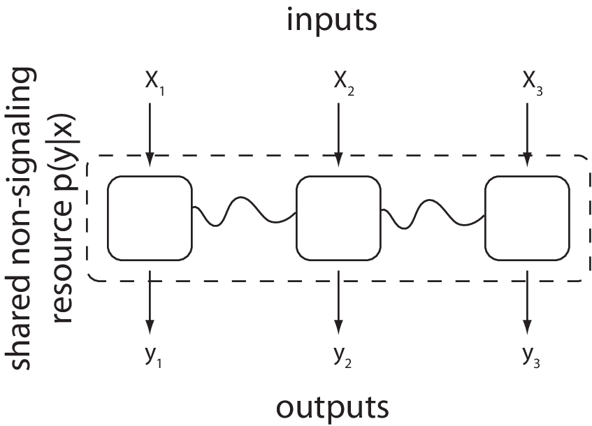
So far, the paradigm of distributed computation assumed communication between the nodes. On the one hand the communication was directly quantified and the cost of communication was measured as in communication complexity problems (see [2] for review). On the other hand some global inputs/outputs processing was performed by a referee [3]. Here we focus on computation without communication.
Namely, we want to address the following question: is quantum mechanics superior to classical theory regarding distributed computation of total function, if no communication between nodes is allowed? We answer this question introducing and studying Identity games (in short Id games, the origin of the name will be clarified later) which may be viewed as special type of Bell inequalities [4]. The setup is depicted in FIG. 1 and described with more details in further part of the paper.
We should here stress the difference between the problem we pose and two existing results/approaches. The first one is “guess your neighbour input” (GYNI) game [5]. GYNI game may be viewed as a distributed computation without communication with global constraints imposed on the input set. In contrast, in our approach, we consider all inputs. Secondly, in [6] the communication complexity problem for two parties was translated into scenario, where the goal of one of the parties is to compute some function without communication, but conditioned on an event that other party will not abort. This conditioning is a form of communication, while in our case there is no communication whatsoever.
Intuitively, computing of some non-trivial distributed function requires signaling. Hence there should not be a difference not only between quantum and classical theories, but also non-signaling theory should not give advantage. As an example we may refer to GYNI game where all inputs are allowed. In that case there is no advantage for non-signaling theories.
In this paper we show that quantum systems are superior to classical ones for bipartite and multipartite scenarios. We find that, for the simplest bipartite systems (i.e. each player has binary input and output) non-signaling theory does not offer advantage. However, if we move to more complicated bipartite setups, we obtain that quantum strategies beat classical ones.
Before we present our results, we discuss how the approach proposed in this paper relates to other frameworks for studying non-locality, in particular to Bell inequalities.
The value of Bell expression is the average probability that some function of parties’ inputs is equal to some function of their outputs 11 1 In some instances may depend also on or the average weighted [7].. The most well studied type of Bell inequalities are so-called XOR games [8]. There, the function is simply XOR of the outcomes of all parties. Celebrated CHSH [9] inequality is the most well known example of this type. The main advantage of XOR games is that they allow to change a more complex function into computing XOR’s. As we said, the goal of distributed computation is to reach a point when no further processing is required. Because in this case is just the identity it is why we call the inequalities of this type Id games (i.e. in the case of total functions).
Strangely this case has been left almost untouched with only one, as mentioned above, exception which is GYNI game [5]. As contrary to GYNI game where partial function is computed, here we focus on the total functions . To our knowledge there are no examples of Bell inequalities of type of Id games for total functions.
In analogy to communication complexity problems [2], these Id games may by viewed as functional games where only one output value is a valid answer for given input . This is in contrast to the relational games (e.g. XOR game) where more than one answer is correct for given input .
As in communication complexity problems, Id games are intended to capture an advantage from using non-local resources in distributed computation. In contrast with communication complexity, we do not measure advantage in terms of communication cost. Actually, no communication between parties is allowed in our approach. We focus on the probability that players return correct output.
This paper is structured as follows: Firstly we formally define Id games and resources that can be used to play them. Then we show various examples with quantum advantage for bipartite scenario and discuss the gap between classical and non-signaling resources. Next we move to tripartite scenario. At the end we show that for a vast majority of the functions the classical resources are practically useless while the no-signalling ones allow for strictly better results. We conclude the paper with a discussion of our results and directions for future research.
In the Method section we present numerical examples, some statistics describing number of nontrivial Id games and other details.
RESULTS
Identity games
We study Bell inequalities in terms of nonlocal games. We consider -player games. Each player receives as an input a private message from referee and returns to him an output . and denote numbers of possible inputs and outputs respectively. Inputs are distributed according to some joint probability distribution on vector consisting of messages sent to each player. The goal for players is to achieve maximal value of functional called winning probability:
| (1) |
where and are some functions of inputs and outputs and define the game, is conditional probability distribution describing the strategy.
In the preparation step, players are informed on the input distribution and functions and . Then they establish common strategy based on the shared resources (classical, quantum, non-signaling). During the game, no communication is allowed between the players. Hence they make their decision on the base of their own inputs and shared resources. We will denote maximal winning probability for classical, quantum and non-signaling resources as respectively. The game is non-trivial if .
In this paper we look for non-trivial Id games which are defined by the requirement that is an identity function. Furthermore we consider only the case where . That leads to winning probability in the form:
| (2) |
Strategies
We describe strategies used by players in terms of generalized probabilistic theories. Players share -partite resources. Each player perform some measurement on his part of the resource. The measurements are performed simultaneously and their results are distributed according to joint conditional probability . The following theories, characterized by the conditions imposed on the , are important for our purposes: (i) classical, (ii) quantum and (iii) non-signaling. In classical theory is a mixture of classical local probabilities according to unknown hidden parameter . Two party resource is of the form
| (3) |
For quantum theory, conditional probability distribution has to be reproduced by local measurements (described by projectors ) performed on the shared quantum state :
| (4) |
In non-signaling theories, the only condition is that cannot signal between players. In formal way this condition is expressed for player as
| (5) |
and similarly for player .
To identify functions which lead to non-trivial Id games, we grouped the functions into equivalence classes invariant under local operations or players reordering. Namely we treat functions and as equivalent if might be obtained from by composition of the following operations: (i) input relabelling; (ii) output relabelling; (iii) output conditioning on local input: player returns as an output ; (iv) players reordering. These operations enabled for significant reduction of problem complexity. Then for one representative function from each equivalence class we obtained and by proper optimisation of (2): (i) is convex combination of extreme strategies which are easy to enumerate, we calculate by maximisation of (2) over that set; (ii) was obtained from linear programming with constraints imposed by no signaling conditions.
For non-trivial Id games we analysed performance of quantum strategies. Since we were not able to provide analytical results, we focused on upper bounding numerically. For this purpose we used semidefinite programming (SDP) an approach introduced in [10, 11]. Beside the upper bound, for some cases we provided also concrete examples of quantum strategy offering advantage over classical ones. For all considered bipartite scenarios these advantage is equal to upper bound obtained from SDP.
In the rest of the paper, for simplicity, we take binary inputs (). The results obtained in this and following section can be generalized to any in a straightforward way.
Two-player games
In the scenarios with binary input (i.e. ), there are functions, however none of them leads to non-trivial Id game.
Three inputs per player - The simplest setup where we can find non-trivial Id games and quantum advantage is the case where each player obtains one of the three input symbols (). There are different functions in that setup which reduce to equivalence classes. There are equivalence classes for which . Together they contain functions. For all of these classes and .
We analyzed some of these classes in more detail looking for quantum strategies which may have advantage over classical ones. Interestingly we found that non-signaling strategies winning the games are equivalent to using PR-Boxes [12] and an explicit example of optimal quantum strategy corresponds to the CHSH Bell experiment [9].
We calculated upper bound for using 2-nd level hierarchies of SDP [10]. The highest bound is about better than classical strategy and reads . In comparison non-signaling strategy has advantage. On the other hand we found that for some classes the bound obtained from SDP is equal (with respect to the numerical precision) to .
The example of function with the highest SDP bound is:
| 0 | 1 | 2 | |
|---|---|---|---|
| 0 | 0,0 | 0,0 | 0,0 |
| 1 | 0,0 | 1,1 | 1,1 |
| 2 | 0,1 | 0,1 | 1,1 |
Each cell refers to the output of function for given input. First and second player’s inputs are in the columns and rows respectively.
Optimal classical strategy for this game is obtained when both players return all the time. Optimal non-signaling strategy is analogical to using PR-Box:
| (6) |
Quantum strategy which is optimal for this game (i.e. its attains the SDP bound [10]) looks as follows: Player 1 outputs deterministically when he gets as an input. Otherwise he relabels his input and plays XOR game with optimal quantum strategy. Player 2 performs analogically with relabeling . Note that, when one of the players return deterministically, another one returns or completely random. Success probability for this strategy is .
However, if we consider another Id game (see Methods section for details), we find that the quantum maximum is attained by using non-maximally entangled two-qubit states.
On the other hand, Id games turn out to be useful as dimension witnesses as well, i.e., they are able to witness Hilbert space dimension [14]. In an Id game given in Methods section the players must share at least three dimensional component spaces for maximum quantum violation to happen.
We also found that the SDP bound is equal to classical limit for functions which were symmetric according to players exchange. As an example we present the following symmetric function:
| 0 | 1 | 2 | |
|---|---|---|---|
| 0 | 0,0 | 0,0 | 1,0 |
| 1 | 0,0 | 1,1 | 1,1 |
| 2 | 0,1 | 1,1 | 0,0 |
An optimal non-signaling strategy is analogical to using PR-box:
| (7) |
The above feature that quantum strategies do not offer advantage over classical ones turns out to be true if the players receives four inputs each (instead of three). However, we found counterexample for the case of five inputs per player (see Methods).
Four inputs per player - Let us now move to the scenario where each of the two players may receive 4 inputs (). This scenario is computationally too costly to classify all different functions and make an exhaustive search for quantum violations. However, it is worthy to highlight a few particular Id games for which we find :
(i) Addition game. Let us define the Id game with the following function
| (8) |
where are assumed to take values in whereas . The above encodes in two bits the result of adding two base-4 integers and in a modulo 4 arithmetic. For this game, we have the success probabilities, , , and . Hence, and beat the classical limit by about and , respectively. Both values represent considerable improvement over the 3-input case discussed previously. The quantum maximum is attained by using a maximally entangled two-qubit state and co-planar measurements which are presented in the Methods section.
(ii) A facet-defining game. It turns out that there exists a 4-input Id game, which defines a facet of the Bell local polytope in the scenario of four binary inputs per party. This game is equivalent to the Bell inequality defined by the paper of Brunner and Gisin [16]. See Methods section for an explicit construction of this game.
Three-player games
Here we consider three-player games with binary inputs (). There are different functions which reduce to equivalence classes. We found equivalence classes (with functions together) for which . According to classification of extremal non-signaling strategies [17], for most of equivalence classes, is achieved by decomposable strategies (i.e. strategies which may be decomposed into PR-box on 2 parties and local deterministic box on the remaining party). More details on the classification of winning strategies are presented in the Methods section.
Here we focus on one game where we can also provide an example of quantum strategy with advantage over classical one. The function for this game may be written as:
| (9) | |||||
| (10) | |||||
| (11) |
In the optimal classical strategy all players return all the time which leads to . Optimal non-signaling strategy decomposes into PR-box shared between player 1 and 2 and deterministic strategy used by player (he always returns ). For that strategy we have .
Inspired by decomposability of optimal non-signaling strategy, we propose the following quantum strategy: player and player apply quantum strategy with maximal success probability for XOR game, i.e. the one optimizing . Player uses deterministic strategy: he returns all the time. Success probability achieved by quantum strategy for 2-player XOR game is . It is easy to see from (9)-(11) that . Only one of two possible outputs winning XOR games is valid for the discussed function, and hence for this quantum strategy we get . This value may be compared with the bound obtained from SDP which reads ( hierarchy of [10, 11]).
Generic advantage of Id games with multiple outcomes
We now argue, that for any number of players, for large enough number of outputs, the no-signaling theories beat the classical ones generically. Specifically, let us define as () to be the number of functions for parties, with , for which the probability of successful implementation within classical (non-signaling) theory is . We show that for any number of parties the ratio goes to zero for increasing . The proof is deferred to the Methods section.
METHODS
Two-player games
Id game using partially entangled states - We show an Id game which allows higher winning probability using partial entangled states than maximally entangled states of any dimension. The game is as follows:
| 0 | 1 | 2 | |
|---|---|---|---|
| 0 | 0,1 | 1,1 | 1,0 |
| 1 | 0,0 | 0,1 | 1,1 |
| 2 | 0,1 | 1,0 | 0,1 |
with and .
Using maximally entangled states (of any dimension), . This value has been certified by using the SDP method introduced in Section 4.2 of [18]. However, the maximum using general quantum resources is , which saturates the SDP upper bound of [10]. In fact, can be attained by using a partially entangled two-qubit state. Hence, the winning probability attainable with maximally entangled states (of any dimension) is strictly smaller than the one using non-maximally entangled qubits.
Id game as a dimension witness - We present here an Id game which allows higher quantum violation if more than two-dimensional systems are considered. Hence, this Id game also gives an example to a dimension witness [14]: Maximum quantum violation does not happen in two dimensional systems. The players have to conduct measurements on at least three dimensional systems for maximum quantum violation to happen. The game is as follows:
| 0 | 1 | 2 | |
|---|---|---|---|
| 0 | 0,1 | 1,1 | 1,0 |
| 1 | 0,1 | 1,1 | 1,1 |
| 2 | 0,1 | 1,0 | 1,0 |
with and . Actually, no quantum violation can be observed for two dimensional systems, however, by using three dimensional systems. This value is certified by SDP hierarchy [10] as well.
Id game performing addition - The function defining the game can be written as
| (12) |
where take values in and , which is represented by the table
| 0 | 1 | 2 | 3 | |
|---|---|---|---|---|
| 0 | 0,0 | 0,1 | 1,0 | 1,1 |
| 1 | 0,1 | 1,0 | 1,1 | 0,0 |
| 2 | 1,0 | 1,1 | 0,0 | 0,1 |
| 3 | 1,1 | 0,0 | 0,1 | 1,0 |
This can be further written as the following Bell functional:
| (13) |
with the CHSH game [9]: , where , where take values in . Due to Tsirelson [13], the quantum maximum for is , from which an upper bound of for easily follows. Interestingly, this upper bound can be obtained by an explicit quantum strategy. Just take the qubit observables , , , and along with the Bell state (where refer to Pauli matrices). This provides for the quantity in Eq. (13). Then choose the rest of the observables as , , , and . These choices maximize the other three CHSH quantities as well saturating the upper bound for .
A facet-defining Id game - The function to be considered is as follows:
| 0 | 1 | 2 | 3 | |
|---|---|---|---|---|
| 0 | 0,1 | 1,0 | 0,0 | 1,0 |
| 1 | 0,1 | 1,1 | 0,1 | 1,1 |
| 2 | 0,0 | 1,1 | 0,0 | 1,0 |
| 3 | 0,0 | 1,0 | 1,0 | 0,0 |
This table translates to the following Bell functional:
| (14) |
where
| (15) |
is equivalent up to input/output relabellings with the expression listed in the appendix of Ref. [16].
The maximum quantum violation is attained by using the Bell state and observables and , , where is the vector of Pauli matrices, and Alice and Bob’s respective Bloch vectors , are given as follows:
| (16) |
and
| (17) |
with and . With these settings, we get for , which agrees with the upper bound on level of the SDP hierarchy. Note that the Bloch vectors (both for Alice and Bob) span the full three-dimensional space. Actually, the measurements attaining cannot be brought to a co-planar form and consequently require the use of complex numbers.
Symmetric Id game with quantum advantage - We present here a symmetric Id game for five inputs per player which offers quantum advantage against classical strategies.
| 0 | 1 | 2 | 3 | 4 | |
|---|---|---|---|---|---|
| 0 | 1,1 | 1,0 | 0,0 | 0,0 | 1,1 |
| 1 | 0,1 | 0,0 | 0,1 | 1,1 | 1,1 |
| 2 | 0,0 | 1,0 | 0,0 | 1,1 | 0,1 |
| 3 | 0,0 | 1,1 | 1,1 | 0,0 | 0,0 |
| 4 | 1,1 | 1,1 | 1,0 | 0,0 | 0,0 |
We found that the quantum maximum is (certified by SDP [10] as well) by performing measurements on a 2-qubit singlet state. The classical bound, on the other hand, is .
Three-player games
Here we provide more detailed description of the numerical results obtained for 3-player Id games. We provide some statistics for and and classification of optimal non-signaling strategies according to [17] for these classes where .
Number of equivalence classes for which given is obtained:
| 0.25 | 45 |
|---|---|
| 0.375 | 23 |
Number of equivalence classes for which given is obtained:
| 0.275 | 1 |
| 0.28125 | 1 |
| 0.291667 | 11 |
| 0.3 | 1 |
| 0.3125 | 30 |
| 0.333333 | 1 |
| 0.4375 | 21 |
| 0.5 | 2 |
The difference between and with the number of equivalence classes where it occurs:
| 0.025 | 1 |
| 0.03125 | 1 |
| 0.041667 | 11 |
| 0.05 | 1 |
| 0.0625 | 51 |
| 0.083333 | 1 |
| 0.125 | 2 |
Similar list for relative differences between and :
| 0.1 | 1 |
| 0.125 | 1 |
| 0.166666667 | 21 |
| 0.166668 | 11 |
| 0.2 | 1 |
| 0.25 | 30 |
| 0.333332 | 1 |
| 0.333333333 | 2 |
We do not present statistics for SDP bound of since numerical inaccuracy make it hard to group them into classes.
Since non-signaling strategies which achieve for given are extremal points of non-signaling polytope, we may apply classification from [17] to them. We found that optimal strategies belong to the following classes:
| class | |
|---|---|
| 2 | 53 |
| 19 | 1 |
| 25 | 6 |
| 29 | 6 |
| 31 | 1 |
| 33 | 1 |
There may be also strategies from the other classes since we just checked to which class belongs the strategy obtained from linear programming. Strategies from class may be decomposed into PR-box on parties and local deterministic box on the remaining party. Strategies from classes and are optimal for GYNI game.
Decomposable strategies were discussed in the main part of the paper. Here we give an example of optimal strategy which belongs to class .
The function of the game is given by equations:
| (18) | |||||
| (19) | |||||
| (20) |
Classical and non-signaling strategies optimal for that game achieve , respectively which give the gap , . SDP bound for is
In optimal classical strategy once again all players return all the time while optimal non-signaling strategy has the form (we bolded the entries which win the game):
| 000 | 001 | 010 | 011 | 100 | 101 | 110 | 111 | |
|---|---|---|---|---|---|---|---|---|
| 000 | 1/3 | 0 | 1/3 | 0 | 0 | 0 | 0 | 1/3 |
| 001 | 1/3 | 0 | 0 | 1/3 | 0 | 0 | 1/3 | 0 |
| 010 | 1/3 | 0 | 1/3 | 0 | 0 | 0 | 0 | 1/3 |
| 011 | 1/3 | 0 | 0 | 1/3 | 0 | 0 | 1/3 | 0 |
| 100 | 0 | 0 | 1/3 | 1/3 | 1/3 | 0 | 0 | 0 |
| 101 | 0 | 0 | 1/3 | 1/3 | 1/3 | 0 | 0 | 0 |
| 110 | 1/3 | 0 | 0 | 1/3 | 0 | 0 | 1/3 | 0 |
| 111 | 1/3 | 0 | 0 | 1/3 | 0 | 0 | 1/3 | 0 |
Generic advantage of Id games for no-signalling theories
We will now argue, that for any number of players, for large enough number of outputs, the no-signaling theories beat the classical ones generically. Specifically, let us define as () to be the number of functions for parties, with , for which probability of successful implementation within classical (non-signaling) theory is . We will show:
For any number of parties the ratio goes to zero for increasing .
To prove the claim, let us first note that, for any function , non-signalling theories allow to be at least (so that is actually the number of all functions). This is achieved by a box defined as follows. Let . Define the probability distribution of the box to be
It is straightforward to check that this box is non-signalling and the probability that is exactly for any input. =
Let us now turn to classical theory. Obviously for any function we can have . It is realized by a strategy in which all parties return random outputs regardless of their inputs. There are possible functions . This number comes from the fact that for each function we need to specify the outcome for each of players for any combination of possible inputs. We want to show that for a vast majority of functions the classical resources (shared randomness and local computation) do not allow to reach a significantly higher probability. More precisely, our aim is to find (an upper bound on) – the number of functions with the average success probability of the best classical strategy larger or equal to particular .
One nice property of the classical average success probability is that there exists optimal strategy which is deterministic. (cf. [19]) – namely each party applies function to his input , . Therefore, we can limit ourselves to considering only such strategies.
To enumerate all functions with success probability we need bits. One of the possible ways of enumeration is first to describe the optimal strategies. To do so one needs to describe all the functions . There are functions for every , which gives sets of different functions. Then one can calculate the outputs of this strategy . To fully characterize one can simply take the description of the classical strategy, which requires bits, and append to it a list of numbers . Where is bitwise subtraction modulo . However, each of numbers is equal to 0 whenever the classical strategy succeeds, which happens with probability . There are numbers which need to be specified and each of them has -letter alphabet, but because 0 will appear with probability the entropy of the whole set of ’s is at most , where . is Shannon’s binary entropy and is the highest entropy a variable with -letter alphabet can have if one of the letters has probability . It can be considered a generalization of . is equal to only if and is strictly smaller otherwise.
This encoding uses
| (24) |
bits. Since any encoding must require at least , then , which gives an upper bound on . An important implication is that for any the ratio goes to 0 as goes to infinity. This means that as the size of the input grows the fraction of functions where the classical resources provide a non-negligible advantage over producing random outputs goes to zero which proves the claim.
We actually proved more: for a majority of the functions non-signalling resources can achieve a success rate times higher than the classical ones.
DISCUSSION
In this work, we addressed the following question: is quantum mechanics superior to classical theory regarding distributed computation of total function, if no communication between nodes is allowed? In order to answer this question we introduced Id games. The motivation for the studies of these games comes from the fact that they are instances of a complete nonlocal computation. In the case of any type of distributed computation any exclusions of some possible combinations of inputs for the parties are difficult to justify. Therefore, the functions that we consider are total functions. Moreover, function is defined such that only one output value is a valid answer for a given input . This research has also been partially inspired by the results of [5] where the authors study a particular family of inequalities that is similar to Id games but defined for partial functions (i.e. there is a promise on the players’ inputs). The results from [5] have been very useful in the studies of the foundations of the quantum theory [20, 21] and we believe that Id games will too.
Acknowledgements
This work was supported by the ERC AdG grant QOLAPS, EC grant RAQUEL (323970) and National Science Centre project Maestro DEC-2011/02/A/ST2/00305. M.P was supported by NCN grant 2013/08/M/ST2/00626 and FNP TEAM programme.
References
- [1] P. W. Shor, Polynomial-Time Algorithms for Prime Factorization and Discrete Logarithms on a Quantum Computer, SIAM J. Sci. Statist. Comput. 26 1484 (1997). Preprint at http://arXiv.org/abs/quant-ph/9508027 (1995).
- [2] H. Buhrman, R. Cleve, S. Massar, R. de Wolf, Nonlocality and Communication Complexity, Rev. Mod. Phys. 82 665 (2010). Preprint at http://arXiv.org/abs/0907.3584 (2009).
- [3] N. Linden, S. Popescu, A. J. Short, A. Winter, Quantum Nonlocality and Beyond: Limits from Nonlocal Computation, Phys. Rev. Lett. 99, 180502 (2007). Preprint at http://arXiv.org/abs/quant-ph/0610097 (2006).
- [4] N. Brunner, D. Cavalcanti, S. Pironio, V. Scarani, S. Wehner, Bell nonlocality, Rev. Mod. Phys. 86, 419 (2014).
- [5] M. Almeida, J.-D. Bancal, N. Brunner, A. Acin, N. Gisin, and S. Pironio, Guess Your Neighbors Input: A Multipartite Nonlocal Game with No Quantum Advantage, Phys. Rev. Lett. 104, 230404 (2010).
- [6] I. Kerenidis, S. Laplante, V. Lerays, J. Roland, D. Xiao, Lower bounds on information complexity via zero-communication protocols and applications, In 53rd Annual IEEE Symposium on Foundations of Computer Science (FOCS’12), pages 500–509 (2012).
- [7] D. Collins, N. Gisin, A relevant two qubit Bell inequality inequivalent to the CHSH inequality, J. Phys. A: Math. Gen. 37, 1775-1787 (2004).
- [8] R. Cleve, P. Hoyer, B. Toner, and J. Watrous, Consequences and limits of nonlocal strategies, Proc. 19th IEEE Conf. on Computational Complexity, 236-249 (2004).
- [9] J. F. Clauser , M. A. Horne, A. Shimony, R. A. Holt, Proposed Experiment to Test Local Hidden-Variable Theories, Phys. Rev. Lett. 23, 880 (1969).
- [10] M. Navascues, S. Pironio, A. Acin, Bounding the Set of Quantum Correlations, Phys. Rev. Lett. 98, 010401 (2007).
- [11] M. Navascues, S. Pironio, A. Acin, A convergent hierarchy of semidefinite programs characterizing the set of quantum correlations, New J. Phys. 10, 073013 (2008).
- [12] S. Popescu and D. Rohrlich, Quantum nonlocality as an axiom, Found. Phys. 24, 379–385 (1994).
- [13] B. S. Tsirelson, Quantum generalizations of Bell’s inequality, Lett. Math. Phys., 4 93-100, (1980).
- [14] N. Brunner, S. Pironio, A. Acin, N. Gisin, A. A. Méthot, V. Scarani, Testing the Dimension of Hilbert Spaces, Phys. Rev. Lett. 100, 210503 (2008).
- [15] M. Navascués, G. de la Torre, T. Vértesi, Characterization of Quantum Correlations with Local Dimension Constraints and Its Device-Independent Applications, Phys. Rev. X 4, 011011 (2014).
- [16] N. Brunner, N. Gisin, Partial list of bipartite Bell inequalities with four binary settings, Phys. Lett. A 372, 3162 (2008).
- [17] S. Pironio, J.-D. Bancal, V. Scarani, Extremal correlations of the tripartite no-signaling polytope, J. Phys. A 44, 065303 (2011).
- [18] B. Lang, T. Vértesi, M. Navascués, Closed sets of correlations: answers from the zoo, preprint at http://arXiv.org/abs/1402.2850 (2014).
- [19] A. Fine, Hidden Variables, Joint Probability, and the Bell Inequalities, Phys. Rev. Lett. 48, 291 (1982).
- [20] R. Gallego, L. E. Wurflinger, A. Acin, M. Navascues, Quantum Correlations Require Multipartite Information Principles, Phys. Rev. Lett. 107, 210403 (2011).
- [21] T. Fritz, A. B. Sainz, R. Augusiak, J. B. Brask, R. Chaves, A. Leverrier, A. Acín, Local orthogonality as a multipartite principle for quantum correlations, Nat. Commun. 4, 2263 (2013).