Inert Extension of the Zee-Babu Model

We extend the two-loop induced radiative neutrino mass model proposed by Zee and Babu in Ref. [4] so as to contain a DM candidate by introducing an unbroken discrete $Z_{2}$ symmetry. The particle contents and the charge assignment are shown in Table 1. We add vector-like charged leptons $E_{R}^{\alpha}$ and $E_{L}^{\alpha}$ with three flavours; i.e., $\alpha=$1-3. For the scalar sector, we introduce an $SU(2)_{L}$ doublet $\eta$, singly-charged singlet $\chi^{\pm}$ and doubly-charged singlet $\kappa^{\pm\pm}$ fields. Among these new fields, only $\kappa^{\pm\pm}$ are assigned to be $Z_{2}$ even. A DM candidate can then be obtained as the lightest neutral $Z_{2}$ odd particle; namely, a neutral component of $\eta$.

New terms in the Lagrangian for lepton Yukawa interactions and the scalar potential under the $SU(2)_{L}\times U(1)_{Y}\times Z_{2}$ invariance are given by

where $y_{L}$ and $y_{R}$ are the symmetric $3\times 3$ complex matrices. In the scalar potential, $\mu$, $\mu_{\kappa}$ and $\lambda_{5}$ can be chosen to be real without any loss of generality by renormalizing the phases to scalar bosons. Notice here that although the $(\overline{e^{ci}_{R}}e_{R}^{j}\kappa^{++}+\text{h.c.})$ terms are allowed in general³³ 3 We can forbid these terms by introducing an additional $U(1)$ symmetry. However, such a symmetry also forbids the $\lambda_{5}$ term in the potential in Eq. (II.2) which is necessary to avoid the constraint from the direct detection experiment for DM., they do not contribute to neutrino mass generations. We thus neglect these terms for simplicity throughout the paper.

After the electroweak symmetry breaking, the scalar fields can be parameterized as

where $v~\simeq 246$ GeV is the vacuum expectation value (VEV) of the Higgs doublet, and $G^{\pm}$ and $G^{0}$ are respectively the Nambu-Goldstone bosons which are absorbed by the longitudinal components of $W^{\pm}$ and $Z$ bosons. The other scalar fields are not supposed to have a non-zero VEV, otherwise the electromagnetic interactions or $Z_{2}$ symmetry spontaneously breaks down.

The mass of the Higgs boson $h$ is obtained after taking the vacuum condition; i.e., $\partial\mathcal{V}/\partial\Phi|_{\mathrm{VEV}}=0$ just like the SM Higgs boson as $m_{h}^{2}=2\lambda_{1}v^{2}$. In our model, only the singly-charged scalar states $\eta^{\pm}$ and $\chi^{\pm}$ can mix each other among the new scalar bosons. The mass matrix for the singly-charged scalar states $M_{\pm}^{2}$ in the basis of ($\eta^{\pm}$, $\chi^{\pm}$) is given by

The mass eigenstates $H_{1}^{\pm}$ and $H_{2}^{\pm}$ are defined by introducing the mixing angle $\theta$ as

where $\theta$ and the mass eigenvalues are given by

All the other masses of scalar bosons are calculated as

The neutral component of $\eta$ is the unique DM candidate in the model. Taking $\lambda_{5}>0$, the DM can be identified as $\eta_{I}$ which should satisfy the observed thermal relic density [69]. The DM mass is limited as $m_{\eta_{I}}\lesssim 80~\mathrm{GeV}$ and $m_{\eta_{I}}\gtrsim 500~\mathrm{GeV}$ from the constraint of thermal relic density of DM [71, 70]. When the DM is in the low mass region $m_{\eta_{I}}\lesssim 80~\mathrm{GeV}$ (below the $W$ or $Z$ threshold), the main annihilation process is $\eta_{I}\eta_{I}\to h\to f\overline{f}$ where $b\overline{b}$ is dominant in the final state fermions $f\overline{f}$ due to the size of the Yukawa coupling. In addition to the annihilation process, the co-annihilation with $\eta_{R}$ mediated by $Z$ boson, $\eta_{R}\eta_{I}\to Z\to f\overline{f}$ is effective if the mass difference among them is less than around $10\%$. The flavor of the final state fermions are universal unlike the annihilation process. Typically the DM mass should be around the SM Higgs resonance; i.e., $m_{h}/2\simeq 63$ GeV, to satisfy the thermal DM relic density in the low DM mass region. On the other hand, the annihilation processes $\eta_{I}\eta_{I}\to W^{+}W^{-},\,ZZ$ and $hh$ can be dominant when the DM mass is above the thresholds. In the region of the DM mass $80~\mathrm{GeV}\lesssim m_{\eta_{I}}\lesssim 500~\mathrm{GeV}$, the predicted relic density is strongly suppressed since the cross section which is fixed by the gauge coupling is too large. We are interested in the low DM mass region because such a low DM mass is favored from inducing the large muon anomalous magnetic moment as will be discussed later. Thus the DM mass is fixed to $m_{h}/2$ in the following discussion.

There is the constraint from direct detection experiments since the elastic scattering process with nuclei is induced via Higgs boson exchange. The relevant parameters in the model are $\lambda_{3}$ $\lambda_{4}$ and $\lambda_{5}$, and they are roughly restricted as $\lambda_{3}+\lambda_{4}-\lambda_{5}\lesssim 0.03$ in the low DM mass region [71] from the recent LUX experiment [72]. Moreover, magnitude of the mass degeneracy between $\eta_{R}$ and $\eta_{I}$ is constrained because the inelastic scattering process $\eta_{I}N\to\eta_{R}N$ can occur via $Z$ boson exchange if the mass splitting is small enough. The mass splitting as small as $100~\mathrm{keV}$ is typically ruled out from the $Z$ exchange process [73].

We consider the constraints from the electroweak $S$, $T$ and $U$ parameters proposed by Peskin and Takeuchi [74]. The new contributions to the $S$, $T$ and $U$ parameters are given by

where $c_{\theta}\equiv\cos\theta$ and $s_{\theta}\equiv\sin\theta$, and $\alpha_{\mathrm{em}}\simeq 1/137$ is the electromagnetic fine structure constant. The function $F(p^{2};m_{1},m_{2})$ is given by

This function is reduced to the simple form in the case of $p^{2}=0$ as

which gives zero in the case of $m_{1}=m_{2}$. The experimental deviations from the SM predictions in the $S$ and $T$ parameters under $m_{h}=126$ GeV and $U=0$ are given by [75]⁴⁴ 4 Typically, the magnitude of $U_{\text{new}}$ is smaller than 0.01 when the prediction of $S_{\text{new}}$ and $T_{\text{new}}$ parameters are inside the 95% CL allowed region by the data.

where the correlation factor between $S_{\text{new}}$ and $T_{\text{new}}$ is +0.91.

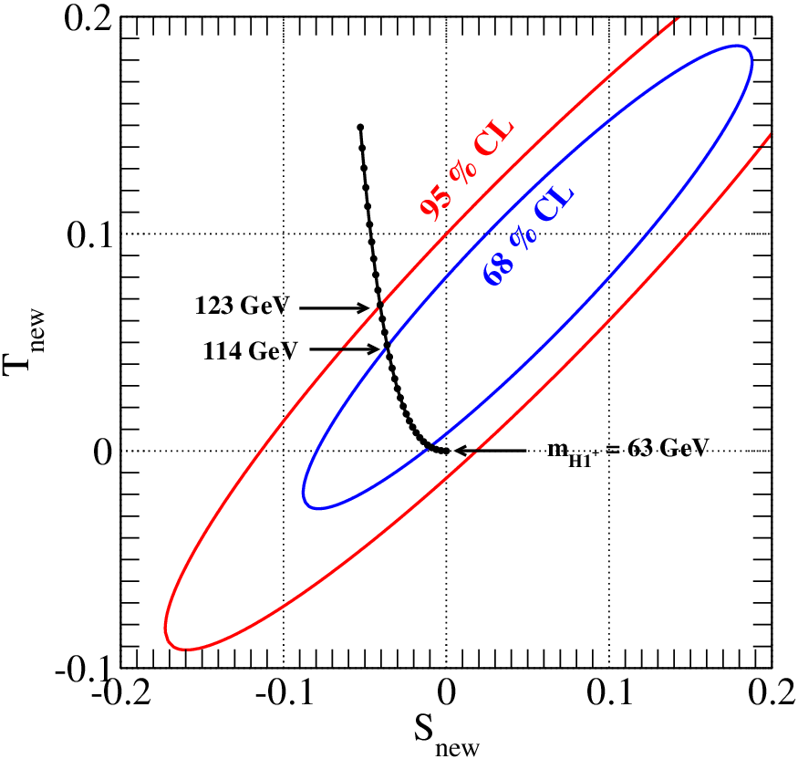
In Fig. 1, we show the prediction of the $S_{\text{new}}$ and $T_{\text{new}}$ parameters. The 68% and 95% CL limits for the $S_{\text{new}}$ and $T_{\text{new}}$ parameters are respectively denoted by the blue and red ellipses. We take $\theta=0$ and $m_{\eta_{R}}=m_{\eta_{I}}=63$ GeV in this plot. In that case, $S_{\text{new}}$ and $T_{\text{new}}$ are determined by fixing $m_{H_{1}^{\pm}}$ which corresponds to the mass of $\eta^{\pm}$. The prediction on the $S_{\text{new}}$-$T_{\text{new}}$ plane changes from the origin to the left-upper edge along the black curve when $m_{H_{1}^{\pm}}$ is valid from 63 GeV to 153 GeV. From this figure, we obtain the upper limit on $m_{H_{1}^{\pm}}$ to be 114 GeV and 123 GeV with the 68% CL and 95% CL, respectively. The upper limit on $m_{H_{1}^{\pm}}$ will be relaxed with several dozens GeV if $U_{\mathrm{new}}\neq 0$ is taken into account [75].

The Majorana neutrino mass matrix $m_{\nu}$ is derived at two-loop level from the diagrams depicted in Fig. 2. The contribution of the left diagram is given by

and that of the right diagram is given by

The loop functions $F_{L}$ and $F_{R}$ are computed as

where

The total neutrino mass matrix is given by $(m_{\nu})_{ij}=(m_{\nu}^{L})_{ij}+(m_{\nu}^{R})_{ij}$. Notice here that the contribution from the left figure in Fig. 2 is reduced to the neutrino mass matrix given in the original Zee-Babu model in the limit of $M_{E^{\alpha}}\to 0$ [76].

When we assume that $y_{\eta}$ is proportional to the unit matrix; i.e., $(y_{\eta})_{i\alpha}=y_{\eta}\times{\bm{1}_{3\times 3}}$, and all the masses for $E^{\alpha}$ are degenerate; $M_{E^{\alpha}}\,(\alpha=1,2,3)=M_{E}$, the neutrino mass matrix is simply rewritten as

where

The neutrino mass matrix is diagonalized by introducing the Pontecorvo-Maki-Nakagawa-Sakata matrix $U_{\text{PMNS}}$ as [77]

By using the following best fit values of the neutrino mixing angles and squared mass differences assuming the normal (inverted) mass hierarchy [78];

we obtain the $U_{\text{PMNS}}$ matrix elements as

where we neglect the CP-violating phase, which is experimentally allowed within the 2-$\sigma$ level [78]. In addition, using the central value of the sum of neutrino masses 0.36 eV [79], the eigenvalues for the neutrino masses are determined in the normal (inverted) hierarchy as

From Eqs. (III.8), (III.1) and (III.14), and taking $y_{L}=y_{R}~(=\bar{y})$, we obtain the matrix elements of $\bar{y}$ in the normal (inverted) hierarchy;

where $m_{\text{max}}$ is the largest eigenvalue of neutrino masses; i.e., $m_{\text{max}}=m_{3}$ ($m_{1}$). The order of magnitude of the parameter $|C_{L}-C_{R}|$ is estimated as

where typical magnitudes of the loop functions $F_{L,R}$ are fixed to be $\mathcal{O}(1)$.

The muon anomalous magnetic moment (muon $g-2$) has been measured at Brookhaven National Laboratory. The current average of the experimental results is given by [80]

It has been well known that there is a discrepancy between the experimental data and the prediction in the SM. The difference $\Delta a_{\mu}\equiv a^{\rm exp}_{\mu}-a^{\rm SM}_{\mu}$ was calculated in Ref. [62] as

and it was also derived in Ref. [63] as

The above results given in Eqs. (III.19) and (III.20) correspond to $3.2\sigma$ and $4.1\sigma$ deviations, respectively.

In our model, there are new contributions to $\Delta a_{\mu}$ as shown in Fig. 3. These contributions are calculated as

where

Under the same assumption taken in the previous subsection, we obtain

where we neglect the mass difference between $\eta_{R}$ and $\eta_{I}$; i.e., $m_{\eta_{R}}=m_{\eta_{I}}\,\equiv m_{\eta^{0}}$.

In Fig. 4, the prediction of $\Delta a_{\mu}$ is shown on the $M_{E}$-$y_{\eta}$ plane in the case of $m_{\eta^{0}}=63$ GeV. From Eqs. (III.19) and (III.20), we can obtain the lower and upper limits on $\Delta a_{\mu}$ as $1.1\times 10^{-9}<\Delta a_{\mu}<5.0\times 10^{-9}$ by allowing up to the $2$-$\sigma$ error. In the blue shaded regions, the prediction is inside the above limit. Furthermore, if we require perturbativity of the coupling constant $y_{\eta}$; i.e., $y_{\eta}^{2}/(4\pi)\leq 1$, the upper limit for $y_{\eta}$ can be set, which is denoted by the horizontal dashed line. When we take the maximal allowed value of $y_{\eta}$ from perturbativity, the region of $150~\text{GeV}\lesssim M_{E}\lesssim 350$ GeV is favored by $\Delta a_{\mu}$. In the next section, we discuss the constraint on $M_{E}$ from the current LHC data.

In the end of this section, we comment on new contributions to the lepton flavor violating (LFV) processes such as $\mu\to e\gamma$ in our model. In general, we can consider diagrams which contribute to the LFV processes by replacing the external muons shown in Fig. 3 with charged-leptons with different flavors with each other. Such a contribution is proportional to the off-diagonal element of the $y_{\eta}$ coupling, so that we can avoid constraints from the LFV data as long as we take the diagonal structure of $y_{\eta}$.

References

- [1] G. Aad et al. [ATLAS Collaboration], Phys. Lett. B 716, 1 (2012) [arXiv:1207.7214 [hep-ex]].
- [2] S. Chatrchyan et al. [CMS Collaboration], Phys. Lett. B 716, 30 (2012) [arXiv:1207.7235 [hep-ex]].
- [3] A. Zee, Phys. Lett. B 93, 389 (1980) [Erratum-ibid. B 95, 461 (1980) ].
- [4] A. Zee, Nucl. Phys. B 264, 99 (1986); K. S. Babu, Phys. Lett. B 203, 132 (1988).
- [5] L. M. Krauss, S. Nasri and M. Trodden, Phys. Rev. D 67, 085002 (2003) [arXiv:hep-ph/0210389].
- [6] E. Ma, Phys. Rev. D 73, 077301 (2006) [hep-ph/0601225].
- [7] P. -H. Gu and U. Sarkar, Phys. Rev. D 77, 105031 (2008) [arXiv:0712.2933 [hep-ph]].
- [8] P. -H. Gu and U. Sarkar, Phys. Rev. D 78, 073012 (2008) [arXiv:0807.0270 [hep-ph]].
- [9] M. Aoki, S. Kanemura and O. Seto, Phys. Rev. Lett. 102, 051805 (2009) [arXiv:0807.0361].
- [10] M. Aoki, S. Kanemura, T. Shindou and K. Yagyu, JHEP 1007, 084 (2010) [Erratum-ibid. 1011, 049 (2010)] [arXiv:1005.5159 [hep-ph]].
- [11] S. Kanemura, O. Seto and T. Shimomura, Phys. Rev. D 84, 016004 (2011) [arXiv:1101.5713 [hep-ph]].
- [12] M. Lindner, D. Schmidt and T. Schwetz, Phys. Lett. B 705, 324 (2011) [arXiv:1105.4626 [hep-ph]].
- [13] S. Kanemura, T. Nabeshima and H. Sugiyama, Phys. Lett. B 703, 66 (2011) [arXiv:1106.2480 [hep-ph]].
- [14] M. Aoki, J. Kubo, T. Okawa and H. Takano, Phys. Lett. B 707, 107 (2012) [arXiv:1110.5403 [hep-ph]].
- [15] S. Kanemura, T. Nabeshima and H. Sugiyama, Phys. Rev. D 85, 033004 (2012) [arXiv:1111.0599 [hep-ph]].
- [16] D. Schmidt, T. Schwetz and T. Toma, Phys. Rev. D 85, 073009 (2012) [arXiv:1201.0906 [hep-ph]].
- [17] S. Kanemura and H. Sugiyama, Phys. Rev. D 86, 073006 (2012) [arXiv:1202.5231 [hep-ph]].
- [18] Y. Farzan and E. Ma, Phys. Rev. D 86, 033007 (2012) [arXiv:1204.4890 [hep-ph]].
- [19] F. Bonnet, M. Hirsch, T. Ota and W. Winter, JHEP 1207, 153 (2012) [arXiv:1204.5862 [hep-ph]].
- [20] K. Kumericki, I. Picek and B. Radovcic, JHEP 1207, 039 (2012) [arXiv:1204.6597 [hep-ph]].
- [21] K. Kumericki, I. Picek and B. Radovcic, Phys. Rev. D 86, 013006 (2012) [arXiv:1204.6599 [hep-ph]].
- [22] R. Bouchand and A. Merle, JHEP 1207, 084 (2012) [arXiv:1205.0008 [hep-ph]].
- [23] E. Ma, Phys. Lett. B 717, 235 (2012) [arXiv:1206.1812 [hep-ph]].
- [24] G. Gil, P. Chankowski and M. Krawczyk, Phys. Lett. B 717, 396 (2012) [arXiv:1207.0084 [hep-ph]].
- [25] H. Okada and T. Toma, Phys. Rev. D 86, 033011 (2012) arXiv:1207.0864 [hep-ph].
- [26] D. Hehn and A. Ibarra, Phys. Lett. B 718, 988 (2013) [arXiv:1208.3162 [hep-ph]].
- [27] P. S. B. Dev and A. Pilaftsis, Phys. Rev. D 86, 113001 (2012) [arXiv:1209.4051 [hep-ph]].
- [28] Y. Kajiyama, H. Okada and T. Toma, Eur. Phys. J. C 73, 2381 (2013) [arXiv:1210.2305 [hep-ph]].
- [29] H. Okada, arXiv:1212.0492 [hep-ph].
- [30] M. Gustafsson, J. M. No and M. A. Rivera, Phys. Rev. Lett. 110, 211802 (2013) arXiv:1212.4806 [hep-ph].
- [31] M. Aoki, J. Kubo and H. Takano, Phys. Rev. D 87, no. 11, 116001 (2013) [arXiv:1302.3936 [hep-ph]].
- [32] Y. Kajiyama, H. Okada and K. Yagyu, Nucl. Phys. B 874, 198 (2013) [arXiv:1303.3463 [hep-ph]].
- [33] Y. Kajiyama, H. Okada and T. Toma, Phys. Rev. D 88, 015029 (2013) [arXiv:1303.7356].
- [34] S. Kanemura, T. Matsui and H. Sugiyama, Phys. Lett. B 727, 151 (2013) [arXiv:1305.4521 [hep-ph]].
- [35] A. E. Carcamo Hernandez, I. d. M. Varzielas, S. G. Kovalenko, H. Päs and I. Schmidt, Phys. Rev. D 88, 076014 (2013) [arXiv:1307.6499 [hep-ph]].
- [36] B. Dasgupta, E. Ma and K. Tsumura, Phys. Rev. D 89, 041702 (2014) [arXiv:1308.4138 [hep-ph]].
- [37] A. E. Carcamo Hernandez, RMartinez and F. Ochoa, arXiv:1309.6567 [hep-ph].
- [38] K. L. McDonald, JHEP 1311, 131 (2013) [arXiv:1310.0609 [hep-ph]].
- [39] S. Baek, H. Okada and T. Toma, JCAP 1406, 027 (2014) [arXiv:1312.3761 [hep-ph]].
- [40] E. Ma, Phys. Lett. B 732, 167 (2014) [arXiv:1401.3284 [hep-ph]].
- [41] A. Ahriche, S. Nasri and R. Soualah, Phys. Rev. D 89, 095010 (2014) [arXiv:1403.5694 [hep-ph]].
- [42] H. Okada, arXiv:1404.0280 [hep-ph].
- [43] A. Ahriche, C. -S. Chen, K. L. McDonald and S. Nasri, arXiv:1404.2696 [hep-ph].
- [44] A. Ahriche, K. L. McDonald and S. Nasri, arXiv:1404.5917 [hep-ph].
- [45] C. -S. Chen, K. L. McDonald and S. Nasri, Phys. Lett. B 734, 388 (2014) [arXiv:1404.6033 [hep-ph]].
- [46] S. Kanemura, T. Matsui and H. Sugiyama, Phys. Rev. D 90, 013001 (2014) [arXiv:1405.1935 [hep-ph]].
- [47] M. Aoki and T. Toma, arXiv:1405.5870 [hep-ph].
- [48] M. Lindner, S. Schmidt and J. Smirnov, arXiv:1405.6204 [hep-ph].
- [49] Y. H. Ahn and H. Okada, Phys. Rev. D 85, 073010 (2012) [arXiv:1201.4436 [hep-ph]].
- [50] E. Ma, A. Natale and A. Rashed, Int. J. Mod. Phys. A 27, 1250134 (2012) [arXiv:1206.1570 [hep-ph]].
- [51] Y. Kajiyama, H. Okada and K. Yagyu, JHEP 10, 196 (2013) arXiv:1307.0480 [hep-ph].
- [52] Y. Kajiyama, H. Okada and K. Yagyu, arXiv:1309.6234 [hep-ph].
- [53] E. Ma, Phys. Rev. Lett. 112, 091801 (2014) [arXiv:1311.3213 [hep-ph]].
- [54] E. Ma and A. Natale, Phys. Lett. B 723, 403 (2014) [arXiv:1403.6772 [hep-ph]].
- [55] H. Okada and K. Yagyu, Phys. Rev. D 89, 053008 (2014) [arXiv:1311.4360 [hep-ph]].
- [56] S. Baek, H. Okada and T. Toma, Phys. Lett. B 732, 85 (2014) [arXiv:1401.6921 [hep-ph]].
- [57] H. Okada and K. Yagyu, arXiv:1405.2368 [hep-ph].
- [58] D. Schmidt, T. Schwetz and H. Zhang, arXiv:1402.2251 [hep-ph].
- [59] H. N. Long and V. V. Vien, Int. J. Mod. Phys. A 29, no. 13, 1450072 (2014) [arXiv:1405.1622 [hep-ph]].
- [60] V. Van Vien, H. N. Long and P. N. Thu, arXiv:1407.8286 [hep-ph].
- [61] J. Herrero-Garcia, M. Nebot, N. Rius and A. Santamaria, arXiv:1402.4491 [hep-ph].
- [62] F. Jegerlehner and A. Nyffeler, Phys. Rept. 477, 1 (2009) [arXiv:0902.3360 [hep-ph]].
- [63] M. Benayoun, P. David, L. Delbuono and F. Jegerlehner, Eur. Phys. J. C 72, 1848 (2012) [arXiv:1106.1315 [hep-ph]].
- [64] T. P. Cheng and L. -F. Li, Phys. Rev. D 22, 2860 (1980).
- [65] J. Schechter and J. W. F. Valle, Phys. Rev. D 22, 2227 (1980).
- [66] G. Lazarides, Q. Shafi and C. Wetterich, Nucl. Phys. B 181, 287 (1981).
- [67] R. N. Mohapatra and G. Senjanovic, Phys. Rev. D 23, 165 (1981).
- [68] M. Magg and C. Wetterich, Phys. Lett. B 94, 61 (1980).
- [69] P. A. R. Ade et al. [ Planck Collaboration], arXiv:1303.5076 [astro-ph.CO].
- [70] T. Hambye, F. -S. Ling, L. Lopez Honorez and J. Rocher, JHEP 0907, 090 (2009) [Erratum-ibid. 1005, 066 (2010)] [arXiv:0903.4010 [hep-ph]].
- [71] L. Lopez Honorez, E. Nezri, J. F. Oliver and M. H. G. Tytgat, JCAP 0702, 028 (2007) [hep-ph/0612275].
- [72] D. S. Akerib et al. [LUX Collaboration], arXiv:1310.8214 [astro-ph.CO].
- [73] D. Tucker-Smith and N. Weiner, Phys. Rev. D 64, 043502 (2001) [hep-ph/0101138].
- [74] M. E. Peskin and T. Takeuchi, Phys. Rev. Lett. 65, 964 (1990); M. E. Peskin and T. Takeuchi, Phys. Rev. D 46, 381 (1992).
- [75] M. Baak, M. Goebel, J. Haller, A. Hoecker, D. Kennedy, R. Kogler, K. Moenig and M. Schott et al., Eur. Phys. J. C 72, 2205 (2012) [arXiv:1209.2716 [hep-ph]].
- [76] D. Aristizabal Sierra and M. Hirsch, JHEP 0612, 052 (2006) [hep-ph/0609307].
- [77] Z. Maki, M. Nakagawa and S. Sakata, Prog. Theor. Phys. 28, 870 (1962).
- [78] D. V. Forero, M. Tortola and J. W. F. Valle, arXiv:1405.7540 [hep-ph].
- [79] F. Beutler et al. [BOSS Collaboration], arXiv:1403.4599 [astro-ph.CO].
- [80] G. W. Bennett et al. [Muon G-2 Collaboration], Phys. Rev. D 73, 072003 (2006) [hep-ex/0602035].
- [81] [ATLAS Collaboration], Report No. ATLAS-CONF-2013-049.
- [82] A. Pukhov, [hep-ph/0412191].
- [83] K. S. Babu and C. Macesanu, Phys. Rev. D 67, 073010 (2003) [hep-ph/0212058].
- [84] M. Nebot, J. F. Oliver, D. Palao and A. Santamaria, Phys. Rev. D 77, 093013 (2008) [arXiv:0711.0483 [hep-ph]].
- [85] P. Fileviez Perez, T. Han, G. -y. Huang, T. Li and K. Wang, Phys. Rev. D 78, 015018 (2008) [arXiv:0805.3536 [hep-ph]].
- [86] C. -W. Chiang, T. Nomura and K. Tsumura, Phys. Rev. D 85, 095023 (2012) [arXiv:1202.2014 [hep-ph]].
- [87] S. Kanemura, K. Yagyu and H. Yokoya, Phys. Lett. B 726, 316 (2013) [arXiv:1305.2383 [hep-ph]].
- [88] Z. Kang, J. Li, T. Li, Y. Liu and G. -Z. Ning, arXiv:1404.5207 [hep-ph].
- [89] S. Kanemura, M. Kikuchi, K. Yagyu and H. Yokoya, arXiv:1407.6547 [hep-ph].