The double formation of primordial black holes
Abstract
Primordial black holes (PBHs) are a useful tool in cosmology to probe primordial inhomogeneities on small scales that reenter the Hubble radius during the radiation dominated epoch. In this paper, a phenomenon we call the double formation of PBHs, described below, is explored. Suppose there exists a highly perturbed region which will collapse to form a PBH after the horizon crossing of this region, and farther that this region is superposed on much larger region, which also collapses upon reentry. One then expects the collapse of the central smaller region at the time of the crossing of this region, followed by another collapse of the larger perturbation at the time of its respective crossing. The smaller PBH, formed earlier, should be swallowed in the second collapse leading to a single larger PBH as the final state. This paper reports the first direct numerical confirmation of such double PBH formation. Related to this, we also discuss the effects of high-frequency modes on the formation of PBHs.
I introduction
Any large amplitude perturbation of order unity can collapse to a primordial black hole (PBH) in the radiation-dominated universe after the horizon crossing[1, 2]. The mass of PBHs is of the order of the horizon mass at the horizon crossing and therefore can span a wide range between g and 11 1 Recently, constraints on PBHs as the seeds of supermassive and intermediate mass black holes are discussed [3]. .
PBHs with different masses can lead to different observational signals, leading to a vast amount of literature in this field. So far there has been no conclusive evidence of the existence of PBHs, and observational upper bounds on the abundance on various mass scales have been obtained, which are updated and summarized in [4] together with new constraints imposed by Hawking radiation [5]. In the following, we mention several of these.
PBHs smaller than g would have evaporated by now through Hawking radiation, emitting high-energy particles, which can change the history of Big-Bang Nucleosynthesis [6, 7, 8, 9, 10, 11]. In addition, these high-energy particles could be observed as the gamma-ray background [12, 13, 14] or galactic and extragalactic antiprotons [15].
Larger PBHs would still exist today and are constrained by lensing effects [16]. Also, PBHs can be constrained by the stochastic gravitaional wave background for the following reason. When PBHs are formed in large numbers, the typical amplitude of primordial inhomogeneities is faily large [17, 18] (note that the amplitude is on largerst observable scales , relevant to CMB or large-scale structure). In this case, large amplitude tensor perturbations are generated due to the second-order effects of scalar perturbations (induced gravitational waves), potentially leading to observational imprints in the stochastic gravitational wave background [19, 20].
PBHs are important partly because they may explain dark matter. Up until recently, there has been a ”window” of mass scales of PBH dark matter, g-g [4], namely, PBHs in this mass range have been a viable candidate of dark matter. However, more recently, progress has been made in the observational constraint of PBHs in this window. Several authors have claimed that the possibility of PBHs being all the dark matter has been excluded based on micro-lensing [21] and PBH capture by neutron stars [22, 23] and stars [24]. Therefore, the window for PBH dark matter has been narrowed substantially. However, this is not the whole story. Several authors have claimed that Hawking radiation stops when the mass of PBHs reaches the Planck mass, with so called ”Planck mass relics” left, and these relics can also provide a viable candidate of dark matter [13] (see also [4] and references therein). It would be fair to say that the relative importance of Planck mass relics being dark matter has been increased since the aforementioned window has been diminishing, and so further exploration of this possibility is much awaited.
Observational upper bounds on PBHs provide valuable information on inflationary models [25, 26, 27, 28], predicting generation of super-horizon curvature perturbations [29, 30, 31, 32]. So far, primordial perturbations on largest observable scales have been precisely probed by CMB [33, 34] and large-scale structure [35]. It is equally important to probe primordial inhomogeneities on significantly smaller scales in order to help pinpoint the correct inflationary model. Indeed, there exist a number of inflationary models that predict the enhancement of the power spectrum at small scales [36, 37, 38, 39, 40, 41, 42, 43, 44, 45, 46, 47, 48, 49, 50, 51, 52, 53, 54]. PBHs provide one of the important proves of primordial inhomogeneities on small scales (others include CMB distortions [55], ultracompact minihalos [56], acoustic reheating [57]).
In order to use PBHs as a reliable tool in cosmology, precise knowledge of their formation condition is required. A considerlation of the balance between gravity and pressure gradients, which hamper contraction, yielded a simple analytic criterion of PBH formation [58, 59], where is the energy density perturbation averaged over the overdense region evaluated at the time of horizon crossing in the uniform Hubble slice. This criterion has long been used in predicting PBH abundance (but has recently been analytically refined in [60]). In this simple picture the dependence on the profile or shape of perturbed regions has not been taken into account.
Recent numerical analyses, however, have shown that the condition for PBH formation does depend on the profile of perturbation [61, 62] (see also [63, 64] for earlier work). In these papers, some functions were introduced to model primordial perturbed regions and obtained conditions for PBH formation. However, their functions include at most two parameters and therefore the types of initial perturbation profiles investigated were limited. In reality, various kinds of perturbations must have been generated during inflation so in our previous paper [65] (hereafter NHPY) we considered a considerably wider class of perturbations by introducing a function including as many as five parameters. For this extended class of shapes, we have found that the condition for PBH formation is generically expressed by two quantities characterizing profiles of perturbations; one is presented as an integral of curvature over initial configurations and the other is presented in terms of the position of the boundary and the edge of the core, which may measure the effects of pressure gradients.
It turns out that the function introduced in NHPY enables us to investigate a phenomenon we call the double formation of PBHs. Suppose there exists a highly perturbed region which will collapse to form a PBH after horizon crossing, and also that this region is superposed on a much larger region, which also collapses as it enters the horizon later. Then, the collapse of the central smaller region at the time of the crossing should be followed by another collapse of the larger perturbation at the time of the crossing of this larger perturbation. The smaller PBH, formed earlier, is involved in the second collapse leading to a larger PBH as the final state. It is expected that the first collapse is not significantly affected by the presence of the larger perturbation since it is still outside the horizon at the time of the crossing of the smaller perturbation 22 2 Relate to this issue, in [66], it is argued that one should focus on the density contrast on comoving slices to correctly calculate PBH abundance, considering the existence of super-horizon modes of the curvature perturbation. . This paper is aimed at reporting a first direct numerical confirmation of this phenomenon of double PBH formation 33 3 This phenomenon is an analogue of situations where a dark matter halo, formed at some time, becomes a part of a larger halo later, in the process of large-scale structure formation. These situations are taken into account in Press-Schechter formalism [67]. This issue has been discussed in the literature in the context of PBHs as well, for example in [59]. But it may be interesting to note the difference between the halo and PBH case. In the case of dark matter halos, a given halo is destined to be involved in a larger halo and this process takes place continuously; a halo forms at some time and in the next instant this halo becomes a part of a slightly larger halo. This is because perturbations of the dark matter always grow and the formation of a halo is determined solely by whether the amplitude of the density perturbation, smoothed over each scale, exceeds the threshold value (for the spherical case), irrespective of the timing (in this case the notion of the horizon crossing does not play any role since the halo formation takes place well inside the horizon). For the case of PBHs, the double-(or potentially multiple-)formation does not always take place, and when it happens it happens basically discretely (the next PBH formation, involving another smaller PBH or PBHs inside, takes place after some finite time interval). This is because whether a perturbation collapses to form a PBH has already been determined by the time of the horizon crossing, and if it does not collapse, it disperses completely. .
In the double formation of PBHs, from the smaller PBH perspective, one is simply swallowed by the larger PBH. But from the point of view of the larger PBH, the presence of the smaller-scale perturbation leading to the smaller PBH corresponds to the existence of a high-frequency mode (hereafter a HF mode), whose wavelength is much shorter than the perturbed region under consideration. In numerical simulations of the formation of PBHs, the presence of HF modes has not been taken into account [61, 62, 63, 64, 65]. In reality, HF modes should also exist unless PBHs result from a spike in the primordial power spectrum with extremely small width, and thus affect the formation of PBHs to some extent so investigating this issue is also important to fully understand the dynamics of the PBH formation. This has been numerically investigated for the first time and we find that HF-modes facilitate the formation of PBHs.
The rest of the paper is organized as follows. In §II, we briefly discuss our methods and §III is dedicated to a discussion of the double formation of PBHs. In §IV, the effects of high-frequency modes are discussed and §V is devoted to the conclusion.
II Method
We now review the methods employed. More details can be found in NHPY.
The metric we employ is [68]
| (1) |
where , and are functions of and the time coordinate . We consider a perfect fluid with energy density and pressure with a constant equation-of-state parameter such that . We express the proper time derivative of as
| (2) |
where dots denote derivatives with respect to .
We define the mass, sometimes referred to as the Misner-Sharp mass in the literature, within the shell of circumferential radius by
| (3) |
We consider the evolution of a perturbed region embedded in a flat Friedmann-Lemaitre-Robertson-Walker (FLRW) Universe with metric
| (4) |
which is a particular case of (1). The scale factor in this background evolves as
| (5) |
where is some reference time.
We denote the background solution with a subscript 0. In terms of the metric variables defined in (1), we find
| (6) |
The background Hubble parameter is
| (7) |
and the energy density is calculated from the Friedmann equation,
| (8) |
The energy density perturbation is defined as
| (9) |
The curvature profile is defined by writing as
| (10) |
Note that this quantity vanishes outside the perturbed region so that the solution asymptotically approaches the background FLRW solution at spatial infinity.
We denote the comoving radius of a perturbed region by , the precise definition of which will be given later (see eq. (14)), and define a dimensionless parameter in terms of the squared ratio of the Hubble radius to the physical length scale of the configuration,
| (11) |
When we set the initial conditions for PBH formation, the size of the perturbed region is much larger than the Hubble horizon. This means at the beginning, so it can serve as an expansion parameter to construct an analytic solution of the system of Einstein equations to describe the spatial dependence of all the above variables at the initial moment when we set the initial conditions. In this paper, the second order solution, obtained in [69], is used to provide initial conditions for the numerical computations.
We define the initial curvature profile as
| (12) |
where is an arbitrary function of which vanishes outside the perturbed region. Note that, from (10), has to satisfy the condition
| (13) |
We normalize the radial Lagrangian coordinate in such a way that .
In order to represent the comoving length scale of the perturbed region, we use the co-moving radius, , of the overdense region. We can calculate by solving the following equation for the energy density perturbation defined by (9):
| (14) |
Since the initial condition is taken at the super-horizon regime, when is extremely small, the following lowest-order solution [62]
| (15) |
suffices to calculate , which is obtained by solving
| (16) |
Note that the physical length scale in the asymptotic Friedmann region is obtained by multiplying by the scale factor , the normalization of which we have not specified. We can therefore set up initial conditions for the PBH formation with arbitrary mass scales by adjusting the normalization of which appears in the expansion parameter.
The following equations were used in [70] to analyze the gravitational collapse of spherically symmetric masses:
| (17) |
| (18) |
| (19) |
| (20) |
| (21) |
| (22) |
| (23) |
| (24) |
| (25) |
where and
| (26) |
The constraint equation reads
| (27) |
Boundary conditions are imposed such that and at the center, and on the outer boundary so that the numerical solution is smoothly connected to the FLRW solution.
In this slicing, the computation stops after the horizon is formed due to the appearance of a singularity, so the eventual mass of the PBH can not be determined. The determination of the mass without facing a singularity through the technique of null slicing [71, 72, 73, 64, 74] was also discussed in NHPY. In this slicing, space-time is sliced along the null geodesics of hypothetical photons emitted from the center and reaching a distant observer. In other words, the space-time is sliced with hyper-surfaces, defined by a constant null coordinate , the so-called observer time defined shortly. By this construction of the null slicing, only information outside the horizon is calculated, without looking into what happens inside the apparent horizon. Initial conditions are given on some hypersurface defined by constant and are obtained using the cosmic time slicing by calculating the null geodesic of a hypothetical photon which reaches a distant observer after being emitted from the center at some moment in time, while at the same time recording the physical quantities on this null geodesic [73]. In this slicing, the information can be obtained without facing a singularity until a sufficiently later time when the eventual mass of a PBH can be determined.
Let us define the time variable by first noting
| (28) |
along an outgoing photon. Then is defined by
| (29) |
where is the lapse function necessary to make a perfect differential. From this definition, (28) holds along the hyper-surfaces each defined by constant , meaning that these surfaces correspond to the null geodesics of outgoing photons. Using as the time variable then means that the space-time is sliced with the null slices. A boundary condition on the lapse function is imposed by setting , hence at the surface defined by . The physical meaning of this boundary condition is that is chosen to coincide with the proper time measured by a distant observer residing at spatial infinity in the background FLRW universe. For this reason, the null slicing is also sometimes referred to as observer time slicing in the literature.
The Einstein equations in null slicing were obtained in [71], later used to simulate gravitational collapse followed by the formation of a black hole [72, 73], and to simulate the PBH formation as well [64, 74]. We used numerical techniques similar to those of [73, 74]. The fundamental equations are as follows:
| (30) |
| (31) |
| (32) |
| (33) |
| (34) |
| (35) |
| (36) |
where the subscript denotes differentiation with respect to . Boundary conditions are the same as those in the cosmic time slicing.
III The double formation of PBHs
In NHPY, the following function was introduced to parameterize various types of initial curvature profiles:
| (37) |
Before discussing the double PBH formation, let us first consider a simple case with to demonstrate the results of a numerical computation for the case of a single PBH formation.

The hypersurfaces of const., corresponding to null geodesics, are shown in the left panel of Fig.1. Observe that the intervals between null geodesics are tiny in the central region, meaning that time here is effectively frozen. Therefore, the formation of a singularity can be avoided in this slicing as expected. The upper lines in this figure correspond to the null geodesics of the hypothetical photons which are emitted from the center at later times and feel the effects of stronger gravity, so that they need more time to reach a distant observer. In this figure there is an envelope curve of the null geodesics, which approximately shows the location of the apparent horizon. In this way the time evolution is computed only outside the apparent horizon, so the eventual mass of a PBH can be determined without facing a singularity. From the same figure, the apparent horizon radius can be confirmed to asymptote to a constant value after its formation. This means that the black hole mass asymptotes to a constant value because on the apparent horizon, and this behavior of the mass can be confirmed by the converging curves of the mass profile in the right panel of Fig.1.
The flatness of the mass profile in later times can be understood by noting that the energy density in a region away from the center decreases due to the expansion of the universe and also due to the existence of an underdense region surrounding the central overdense region so that the spacetime approaches the spatially flat FLRW universe. In this example, the eventual mass of the PBH is .
In order to discuss double formation, we consider a profile with , depicted in Fig.2. In this case, the central perturbed region, represented by the first term of (37), is superposed on the perturbed region represented by the second term whose length scale is ten times larger than the central perturbed region. The first term itself corresponds to an initial perturbation which can collapse to form a PBH after the perturbed region crosses the horizon as mentioned earlier. The perturbation represented by the second term is physically equivalent to the following profile, after a scale transformation :
| (38) |
So when , which holds in the current parameter choice, the perturbation represented by the second term is equivalent to the one represented by the first. Therefore, the second term itself can also collapse to form a PBH after horizon crossing without the presence of the first term.

Physically, what is expected to happen from this initial set up is that the central region, represented by the first term, collapses to form a PBH as it enters the horizon and then the larger-scale perturbation represented by the second term collapses to form a larger PBH after this scale crosses the horizon, involving the central smaller PBH already formed earlier.
We confirm this prediction by a numerical computation with the aforementioned initial curvature profile provided as the initial condition; results are shown in Fig.3 and 4. First, a PBH with mass around , where is the horizon-crossing time defined by the first term of (37), is formed, and then another larger PBH is formed. Note that the mass of the smaller PBH is somewhat larger than , the mass of the PBH in the previous case with , even though the first term is equivalent to this case. This is due to the existence of the second term describing the larger scale perturbation, which makes the average density around the central region larger at the time of the formation of the smaller PBH. On the other hand, the mass of the larger PBH is almost 100 times larger than the previous case with , which can be understood as follows. First of all, in this simulation of double formation, the radius of the overdense region is defined by the first term of (37). So let us denote this radius by to be contrasted with , the radius of the overdense region defined by the second term. Since and , we find . Then, denoting the horizon crossing time defined by the first term as , we have from eq.(11). Since the Hubble radius and the horizon mass are proportional to , we find as well as . Hence, the upper right parts of Fig.3 and 4 are obtained by rescaling the left and right panel of Fig.1 by respectively, since the vertical and horizontal axis of the Fig.3 and 4 are normalized by the horizon mass and the Hubble radius at the time of the crossing defined by the first term of eq.(37).


IV The effects of high-frequency modes
In numerical simulations of the formation of PBHs, the presence of high-frequency modes (hereafter HF modes), whose wavelength is much shorter than the perturbed region under consideration, are not taken into account [61, 62, 63, 64, 65]. HF modes, however, should exist since in principle the power spectrum of primordial curvature perturbations has an extended profile and thus affect the formation of PBHs to some extent. In this section, the effects of HF modes are discussed.
To this end, let us introduce the following initial curvature profile:
| (39) |
When , this function represents situations where a HF mode is superposed upon a perturbation of longer wavelength, as is shown in Fig.5.

The time evolution of the energy density perturbation of a typical case is shown in Fig.6.
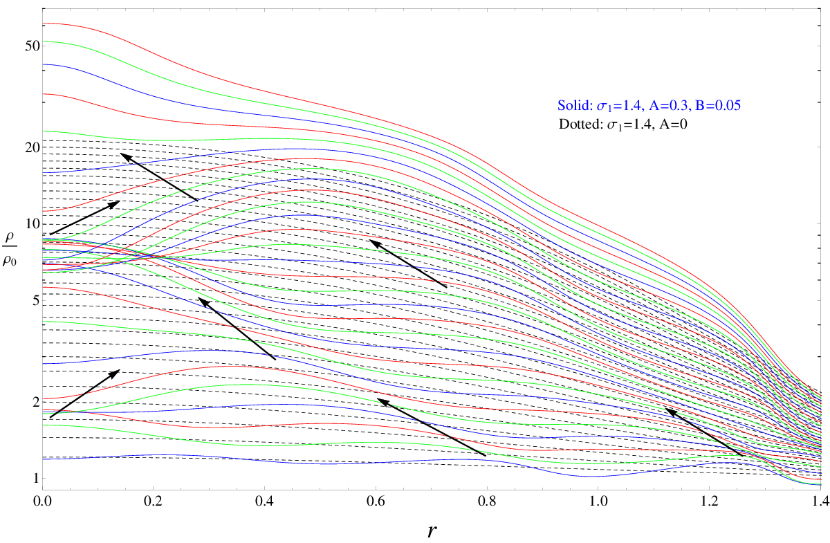
The HF mode crosses the horizon first and starts to grow before the main, or long-wavelength perturbation crosses the horizon. At this point, the main perturbation does not seem present as long as we focus on the density perturbation, since the density perturbation is suppressed on super-horizon scales in the comoving slicing we employ. After the horizon crossing of the main perturbation, the density perturbation with the corresponding wavelength starts to grow, and the HF mode starts to propagate towards the center due to stronger gravity in the center, resulting from the main perturbation. When a local maximum arrives at the center, it bounces, but soon it pulls back towards center once more and as a whole the energy density in the center seems to increase more rapidly than the case without the HF mode. As a result, the value of the density perturbation at the center fluctuates significantly, as is shown in Fig.6 44 4 This makes it difficult to determine (as quickly as possible to reduce computational costs) when the perturbation is destined to die without forming a PBH, the determination which is necessary to investigate the formation condition of PBHs. Without the presence of HF modes, determining when a perturbation is destined to vanish is simple, since in this case the density perturbation at the center monotonically increases when a BH is eventually formed, and once it starts to decrease, the perturbation will definitely die so at this time one can stop numerical integration. In contrast, when a HF mode is present, one cannot conclude the perturbation will decay even if the density perturbation at the center starts to decrease, because it can be due to the presence of the HF mode, as is shown in Fig.6. So careful analysis is required to ensure the quasi-global decrease in the density perturbation before stopping numerical integration in cases including HF modes. .
In Fig.7, the PBH formation condition for this class of profiles is shown, where is fixed to .

For (without the HF mode), the PBH is formed when . When is larger, the threshold value decreases, implying the HF mode somewhat facilitates the formation of PBHs, though one may have expected the HF mode to hinder formation. One may naively suspect such facilitation is simply because, first assuming the local maxima to help PBH formation and local minima to hinder formation, inner local extrema are more effective than outer local extrema and (39) implies the innermost local extremum is a local maximum if is positive, hence the effects of local maxima dominate, leading to a decrease of the threshold for larger values of . It turns out that this is not the case by conducting numerical simulations for negative values of and recovering Fig.7, with the horizontal axis replaced by the absolute value of . That is, the phase of the HF mode is not important.
To understand why HF modes help the formation of PBHs, let us look at Fig.6 once more, showing the local maxima start to move towards the center after horizon crossing of the main perturbation. This behavior seems to result from strong gravity in the center due to the main perturbation. This indicates more effective transportation of radiation towards the center, which may explain the reason for the decrease in the threshold value when a HF mode is present.
In Fig.7, the blue threshold line seems to converge to the line defining the ”unphysical” region, determined by the condition eq.(13). However, what happens for even larger values of is difficult to investigate due to large spatial and time derivatives near the center.
It also turned out that the threshold is insensitive to the wavelength of the HF mode (confirmed in the range ), and that introducing two HF modes at the same time facilitates PBH formation somewhat more.
V Conclusion
First, the double formation of PBHs is discussed, where a smaller PBH is swallowed by another bigger PBH. Suppose there exists a highly perturbed region which will collapse to form a PBH after the horizon crossing of this region, and also that this region is superposed on much larger region, which also collapses, as it enters the horizon later. Then, what should happen is the collapse of the central smaller region at the time of the crossing of this region, which is followed by another collapse of the larger perturbation at the time of the crossing of this larger perturbation. The smaller PBH, formed earlier, is swallowed in the second collapse leading to a single larger PBH as the final state. The first collapse turns out to be insensitive to the presence of the larger perturbation since the larger perturbation is still outside the horizon at that moment. In addition, the second collapse is not affected by the already formed small PBH due to the large scale difference. In this paper we have reported a first numerical confirmation of this phenomenon of the double PBH formation.
Second, the effects of HF-modes on the formation of PBHs are discussed. This issue has been numerically investigated for the first time and, we find that HF-modes facilitate the formation of PBHs, decreasing the threshold value required for the formation of PBHs. This could potentially increase the abundance of PBHs by several orders of magnitude. This is because local small-scale overdensities, superposed on a larger perturbation, fall into the center due to the strong gravity realised by the larger perturbation, leading to more efficient transportation of radiation towards the center.
These results show that the calculation of probability distribution of primordial inhomogeneities is essential to precisely predict the abundance of PBHs.
ACKNOWLEDGMENTS
This work was partially supported by Grant-in-Aid for JSPS Fellow No. 25.8199. The author thanks Jun’ichi Yokoyama for useful comments, reading the manuscript, and continuous encouragement. The author also thanks Kevin Croker for useful comments.
References
- [1] Y. B. Zel’dovich and I. D. Novikov, Sov. Astron. 10, 602 (1967).
- [2] S. Hawking, Mon. Not. Roy. Astron. Soc. 152, 75 (1971).
- [3] K. Kohri, T. Nakama, and T. Suyama (2014), eprint 1405.5999.
- [4] B. Carr, K. Kohri, Y. Sendouda, and J. Yokoyama, Phys. Rev. D 81, 104019 (2010), eprint 0912.5297.
- [5] S. Hawking, Nature 248, 30 (1974).
- [6] Y. B. Zel’dovich, A. A. Starobinskii, M. Y. Khlopov, and V. M. Chechetkin, Sov. Astron. Lett. 3, 110 (1977).
- [7] I. D. Novikov, A. G. Polnarev, A. A. Starobinskii, and Y. B. Zel’dovich, Astron. Astrophys. 80, 104 (1979).
- [8] B. V. Vainer and P. D. Naselskii, Astron. Zh. 55, 231 (1978), [Sov. Astron. 22, 138 (1978).].
- [9] B. V. Vainer, O. V. Dryzhakova, and P. D. Naselskii, Pis ma Astronomicheskii Zhurnal 4, 344 (1978), [Sov. Astron. Lett. 4, 185 (1978).].
- [10] S. Miyama and K. Sato, Prog. Theor. Phys. 59, 1012 (1978).
- [11] K. Kohri and J. Yokoyama, Phys. Rev. D 61, 023501 (2000), eprint astro-ph/9908160.
- [12] D. N. Page and S. Hawking, Astrophys. J. 206, 1 (1976).
- [13] J. H. MacGibbon, Nature 329, 308 (1987).
- [14] J. H. MacGibbon and B. J. Carr, Astrophys. J. 371, 447 (1991).
- [15] B. J. Carr, Astrophys. J. 206, 8 (1976).
- [16] B. Paczynski, Astrophys. J. 304, 1 (1986).
- [17] E. Bugaev and P. Klimai, Phys.Rev. D79, 103511 (2009), eprint 0812.4247.
- [18] A. S. Josan, A. M. Green, and K. A. Malik, Phys.Rev. D79, 103520 (2009), eprint 0903.3184.
- [19] R. Saito and J. Yokoyama, Phys. Rev. Lett. 102, 161101 (2009), [107, 069901(E) (2011).], eprint 0812.4339.
- [20] R. Saito and J. Yokoyama, Prog. Theor. Phys. 123, 867 (2010), [126, 351(E) (2011).], eprint 0912.5317.
- [21] K. Griest, A. M. Cieplak, and M. J. Lehner (2013), eprint 1307.5798.
- [22] F. Capela, M. Pshirkov, and P. Tinyakov, Phys.Rev. D87, 123524 (2013), eprint 1301.4984.
- [23] P. Pani and A. Loeb (2014), eprint 1401.3025.
- [24] F. Capela, M. Pshirkov, and P. Tinyakov (2014), eprint 1403.7098.
- [25] A. G. Polnarev, in Morphological Cosmology, edited by P. Flin and H. W. Duerbeck (1989), vol. 332 of Lecture Notes in Physics, Berlin Springer Verlag, pp. 369–376.
- [26] K. Sato, Mon. Not. Roy. Astron. Soc. 195, 467 (1981).
- [27] A. H. Guth, Phys. Rev. D 23, 347 (1981).
- [28] A. A. Starobinsky, Phys. Lett. B 91, 99 (1980).
- [29] V. F. Mukhanov and G. Chibisov, Sov. Phys. JETP 56, 258 (1982).
- [30] A. H. Guth and S. Pi, Phys. Rev. Lett. 49, 1110 (1982).
- [31] S. Hawking, Phys. Lett. B 115, 295 (1982), revised version.
- [32] A. A. Starobinsky, Phys. Lett. B 117, 175 (1982).
- [33] G. Hinshaw et al. (WMAP Collaboration) (2012), eprint 1212.5226.
- [34] P. Ade et al. (Planck Collaboration) (2013), eprint 1303.5082.
- [35] S. Bird, H. V. Peiris, M. Viel, and L. Verde, Mon.Not.Roy.Astron.Soc. 413, 1717 (2011), eprint 1010.1519.
- [36] J. Garcia-Bellido, A. Linde, and D. Wands, Phys. Rev. D 54, 6040 (1996).
- [37] H. M. Hodges and G. R. Blumenthal, Phys. Rev. D 42, 3329 (1990).
- [38] P. Ivanov, P. Naselsky, and I. Novikov, Phys. Rev. D 50, 7173 (1994).
- [39] J. Yokoyama, Astron. Astrophys. 318:673 (1997).
- [40] J. Yokoyama, Phys. Rev. D 58, 083510 (1998a).
- [41] J. Yokoyama, Phys. Rep. 307, 133 (1998b).
- [42] M. Kawasaki and T. Yanagida, Phys. Rev. D 59, 043512 (1999).
- [43] J. Yokoyama, Prog. Theor. Phys. Suppl. 136, 338 (1999).
- [44] R. Saito, J. Yokoyama, and R. Nagata, J. Cosmol. Astropart. Phys. 2008, 024 (2008).
- [45] A. Taruya, Phys. Rev. D 59, 103505 (1999).
- [46] B. A. Bassett and S. Tsujikawa, Phys. Rev. D 63, 123503 (2001).
- [47] A. M. Green and K. A. Malik, Phys. Rev. D 64, 021301 (2001).
- [48] M. Kawasaki, T. Takayama, M. Yamaguchi, and J. Yokoyama, Mod. Phys. Lett. A22, 1911 (2007).
- [49] T. Kawaguchi, M. Kawasaki, T. Takayama, M. Yamaguchi, and J. Yokoyama, Mon. Not. Roy. Astron. Soc. 388, 1426 (2008), eprint 0711.3886.
- [50] K. Kohri, D. H. Lyth, and A. Melchiorri, JCAP 0804, 038 (2008), eprint 0711.5006.
- [51] L. Alabidi and K. Kohri, Phys.Rev. D80, 063511 (2009), eprint 0906.1398.
- [52] L. Alabidi, K. Kohri, M. Sasaki, and Y. Sendouda, JCAP 1209, 017 (2012), eprint 1203.4663.
- [53] M. Kawasaki, A. Kusenko, and T. T. Yanagida, Phys.Lett. B711, 1 (2012), eprint 1202.3848.
- [54] M. Kawasaki, N. Kitajima, and T. T. Yanagida, Phys.Rev. D87, 063519 (2013), eprint 1207.2550.
- [55] J. Chluba, A. L. Erickcek, and I. Ben-Dayan, Astrophys.J. 758, 76 (2012), eprint 1203.2681.
- [56] T. Bringmann, P. Scott, and Y. Akrami, Phys.Rev. D85, 125027 (2012), eprint 1110.2484.
- [57] T. Nakama, T. Suyama, and J. Yokoyama, Phys.Rev.Lett. 113, 061302 (2014a), eprint 1403.5407.
- [58] B. J. Carr and S. Hawking, Mon. Not. Roy. Astron. Soc. 168, 399 (1974).
- [59] B. J. Carr, Astrophys. J. 201, 1 (1975).
- [60] T. Harada, C.-M. Yoo, and K. Kohri (2013), eprint 1309.4201.
- [61] M. Shibata and M. Sasaki, Phys. Rev. D 60, 084002 (1999), eprint gr-qc/9905064.
- [62] A. G. Polnarev and I. Musco, Class. Quant. Grav. 24, 1405 (2007), eprint gr-qc/0605122.
- [63] D. K. Nadezhin, I. D. Novikov, and A. G. Polnarev, NASA STI/Recon Technical Report N 80, 10983 (1979).
- [64] J. C. Niemeyer and K. Jedamzik, Phys. Rev. D 59, 124013 (1999), URL http://link.aps.org/doi/10.1103/PhysRevD.59.124013.
- [65] T. Nakama, T. Harada, A. Polnarev, and J. Yokoyama, JCAP 2014, 037 (2014b), URL http://stacks.iop.org/1475-7516/2014/i=01/a=037.
- [66] S. Young, C. T. Byrnes, and M. Sasaki (2014), eprint 1405.7023.
- [67] W. H. Press and P. Schechter, Astrophys.J. 187, 425 (1974).
- [68] C. W. Misner and D. H. Sharp, Phys. Rev. 136, B571 (1964).
- [69] A. Polnarev, T. Nakama, and J. Yokoyama, J. Cosmol. Astropart. Phys. 2012, 027 (2012), URL http://stacks.iop.org/1475-7516/2012/i=09/a=027.
- [70] M. M. May and R. H. White, Meth. Comput. Phys. 7, 219 (1967).
- [71] W. C. Hernandez, Jr. and C. W. Misner, Astrophys. J. 143, 452 (1966).
- [72] J. C. Miller and S. Motta, Class. Quant. Grav. 6, 185 (1989), URL http://stacks.iop.org/0264-9381/6/i=2/a=012.
- [73] T. W. Baumgarte, S. L. Shapiro, and S. A. Teukolsky, Astrophys. J. 443, 717 (1995).
- [74] I. Musco, J. C. Miller, and L. Rezzolla, Class. Quant. Grav. 22, 1405 (2005), URL http://stacks.iop.org/0264-9381/22/i=7/a=013.