From Explosive to Infinite-Order Transitions on a Hyperbolic Network

Real-world networks [1, 2, 3] exhibit dramatically distinct phenomenology, with a profound imprint of their geometry on the dynamics, when compared with lattices or mean-field systems. What we now call complex networks, aside from being random, possess geometries dominated by small-world bonds and scale-free degree distributions [4, 5]. These lead to novel, and often non-universal, scaling behaviors unknown for lattices. For example, they exhibit discontinuous transition even in ordinary percolation [6] as exactly solvable realizations of the so-called “explosive” percolation transitions [7, 8, 9, 10, 11, 12, 13]. Unlike the Achlioptas process, it is easy to prove that this discontinuity exists [6, 14], however, its origin results from the network structure, not from a correlated process [7].

Hyperbolic networks combine a lattice geometry with a hierarchy of small-world connections. They were originally proposed as solvable models for complex networks [15, 16, 17, 18, 19]. These recursively defined structures provide deeper insights into small-world effects compared to random networks that otherwise require approximate or numerical methods. Work on percolation [17, 20, 21, 6, 22], the Ising model [23, 15, 24, 25], and the $q$-state Potts model [26, 19] have shown that critical behavior, once thought to be exotic and model-specific [3], can be universally categorized near the transition point [27, 26] for a large class of hyperbolic networks, such as those discontinuous percolation transitions described in Refs. [6, 14]. They exemplify a non-trivial category of the explosive cluster-growth mechanisms leading to the discontinuous transition [28]. Yet, it has been noted that this discontinuity arises only as a non-generic case of the general theory [27], making its prevalence in percolation on hyperbolic networks somewhat surprising.

Here, we illuminate the origin of the explosive percolation transition by investigating the $q$-state Potts model on a simple hyperbolic network, MK1 [6]. The analytic continuation in $q$ [29] reveals that the discontinuity that characterizes the explosive percolation transition related to the limit $q\to 1$, rather than being a special case, persists for all $q<2$. Instead, the Ising ferromagnet ($q=2$) emerges as the singular case between all discontinuous ($q<2$) and all infinite-order transitions ($q>2$), with an infinitely smooth order parameter of the Berezinskii-Kosterlitz-Thouless (BKT) type that is consistent with the theory in Ref. [27]. In particular, with real-space renormalization group (RG), we trace the existence of the discontinuous transition to the non-generic behavior of the critical exponent $y_{h}$ that describes the response of the system to a conjugate external field [6, 19]. This exponent, that is temperature-dependent in these hyperbolic networks, happens to reach its maximum exactly at the critical temperature for $q<2$, resulting in merely quadratic corrections in its local expansion. We argue that this exceptional behavior for $q<2$ is intimately connected with the manner in which geometric, lattice-like features are coupled with the hyperbolic structure.

As a simple and generic member of the class of hyperbolic networks, we consider here MK1, as depicted in Fig. 1. MK1 is recursively generated, starting with two sites connected by a single edge at generation $k=0$. Each new generation combines two sub-networks of the previous generation and adds single edge connecting the end sites. As a result, the $k^{th}$ generation contains $N_{k}=2^{k}+1$ vertices, $2^{k}$ backbone bonds, and $2^{k}-1$ small-world bonds. It is an effectively one-dimensional version of the small-world Migdal-Kadanoff hierarchical diamond lattice [15, 17], which has been used previously to prove the existence of the discontinuous transition in ordinary percolation [6]. Recently, this discontinuity has been studied for a variety of other hyperbolic networks for bond and site percolation in Ref. [14]. Refs. [26, 19] have used MK1 to study the $q$-state Potts model for certain integer values of $q\geq 2$. In principle, to relate the Potts model to percolation at $q\to 1$ first requires a $q$-derivative of the partition function [29]. However, we find that this derivative hardly affects the analytic properties, as we will show below by comparing each quantity obtained for $q\to 1$ with the exactly known percolation results.

In close correspondence to the Ising model on hyperbolic networks discussed in Ref. [24] (see also Ref. [26]), we introduce the following couplings. All variables $x_{i}$ interact with their nearest-neighbors along the backbone with a coupling $K_{0}$ (solid links in Fig. 1), while small-world neighbors interact with a coupling $K_{1}$ (shaded links in Fig. 1). Every $x_{i}$ also experiences a uniform external field $B$. Then, in preparation for applying the renormalization group, the Potts-Hamiltonian can be written as

where $\mathcal{R}$ contains all remaining coupling terms of higher level in the hierarchy while the $x_{i}$ on the backbone can be sectioned into a sequence of three-variable graphlets. These consist of two adjacent lattice-backbone bonds bridged by an arched small-world bond in Fig. 1, each with their own “sectional” Hamiltonian,

Here, $I$ is a constant that fixes the overall energy scale. We conveniently choose new variables, similar to (inverse) “activities" [30], $C=e^{-2I}$, $\quad\kappa=e^{-K_{0}}$, and $\theta=e^{-B}$. Similarly defined are the control parameters of temperature $\mu=e^{-\beta J}$ and field $\eta=e^{-\beta h}$, with $\beta=1/kT$ and $h$ as the external field. The “raw” (unrenormalized) couplings are considered as uniform: $K_{0}=K_{1}=\beta J$, where we fix the energy scale via $J=1$, while $B=\beta h$. However, we find that $K_{1}$ does not change under renormalization and retains its raw value, $e^{-K_{1}}=\mu$, a key distinguishing feature of these hyperbolic networks [24, 27]. Thus, the initial values of the renormalizing activities are $C_{0}=1$, $\kappa_{0}=\mu$, and $\theta_{0}=\eta$. Then, we can rewrite the sectional Hamiltonian as

The RG consists of successively tracing out the central variable $x_{n}$ and expressing the renormalized activities $(C^{\prime},\kappa^{\prime},\theta^{\prime})$ in terms of their priors $(C,\kappa,\theta,\mu)$:

Although the remaining variables $x_{n\pm 1}$ present us with up to $q^{2}$ relations between new and old quantities, only three relations are independent. We can obtain the RG-flow for $(\theta^{\prime},\kappa^{\prime})$ at size $N_{k+1}$ in terms of $(\theta,\kappa)$ at size $N_{k}$,

Note the explicit dependence on the control parameter $\mu$ (temperature), characteristic for these networks [27].

First, we analyze the RG-flow in Eq. (3) in the absence of an external field. For $\eta=1=\theta_{0}$, it remains $\theta_{k}=1$ for all $k>0$ and the RG-flow for the bond-coupling becomes

For the Ising model, $q=2$, Eq. (4) reduces with $\kappa\hat{=}jk$ and $\mu\hat{=}j$ to the equivalent of Eq. (6) in Ref. [26], and for percolation, $q=1$, it reduces with $\kappa\hat{=}1-T$ and $\mu\hat{=}1-p$ to Eq. (1) in Ref. [6].

In the thermodynamic limit $(N_{k\to\infty})$, Eq. (3) provides the fixed points $\kappa^{\prime}=\kappa=\kappa_{\infty}$:

where $\kappa_{\infty}^{+}>\kappa_{\infty}^{-}$, with

The strong-coupling limit $\kappa_{\infty}^{0}=0$ always exists for any $q$. However, the Ising case and the limit of Eq. (5) that corresponds to percolation, both have to be considered with some care. Yet, we easily reproduce Eq. (2) in Ref. [6]. We plot the behavior of $\kappa_{\infty}^{\pm}$ in Fig. 2 as a function of $\mu$ for a range of $q$ that highlights the peculiarities of both cases.

To obtain the thermal exponent $y_{t}$, we calculate the relevant eigenvalues along each branch of the fixed-point lines. The Jacobian of the RG-flow in Eq. (4), evaluated at $\kappa=\kappa_{\infty}$, provides the eigenvalue

Hence, with Eqs. (5), we get

The behavior of the eigenvalues, depicted in Fig. 3, follows closely the description developed for general hyperbolic lattices in Ref. [27].

As Fig. 2 shows, for $q<2$ the critical point is located always at $\mu_{c}=\frac{1}{2}$, such that the relevant thermal scaling exponent [31] $y_{t}=\log_{2}\lambda_{t}^{+}$ is given by

which indicates that $y_{t}$ vanishes for all $q<2$. As the generic theory suggests [27], this linear behavior is to be expected when $\kappa_{\infty}^{+}$ is regular at $\mu=\mu_{c}$ such that it possesses a linear slope, which is satisfied for $q<2$, see Fig. 2. Eq. (7) implies that this will remain true also for percolation, $q=1$, in particular. However, for the Ising ferromagnet, and exactly only at $q=2$, $\lambda_{t}$ in Eq. (7), and hence $y_{t}$, becomes a function of $\kappa_{\infty}^{2}$. Miraculously, at $q=2$ the branch-point in $\kappa_{\infty}$ is placed exactly on the $\kappa=0$-axis at $\mu_{c}$ with $\kappa_{\infty}^{\pm}\sim\pm\sqrt{2\left(\mu-\mu_{c}\right)}$. Both effects combine into a linear correction but a different coefficient,

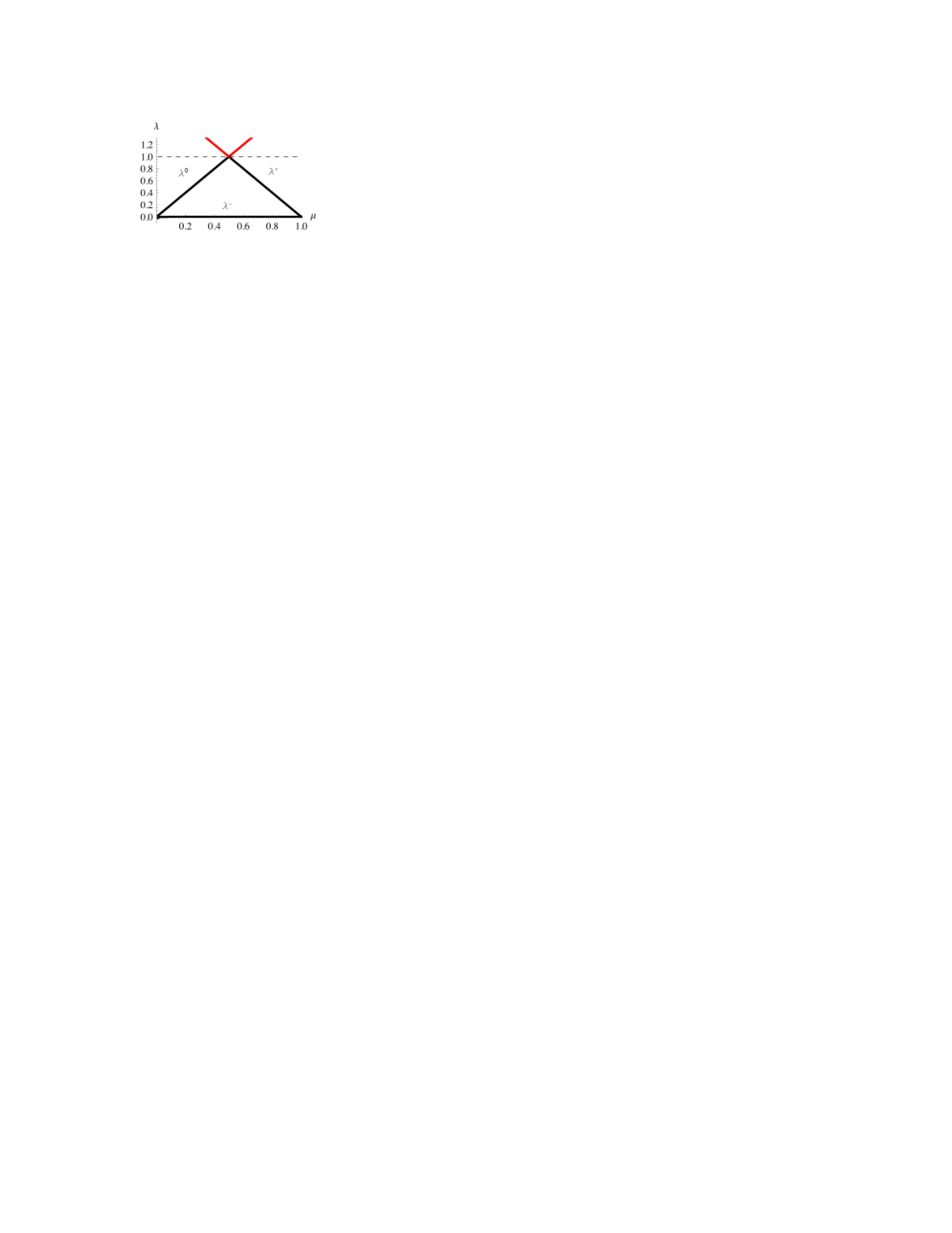
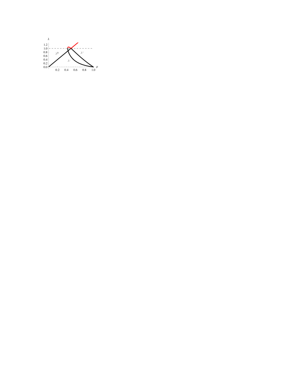
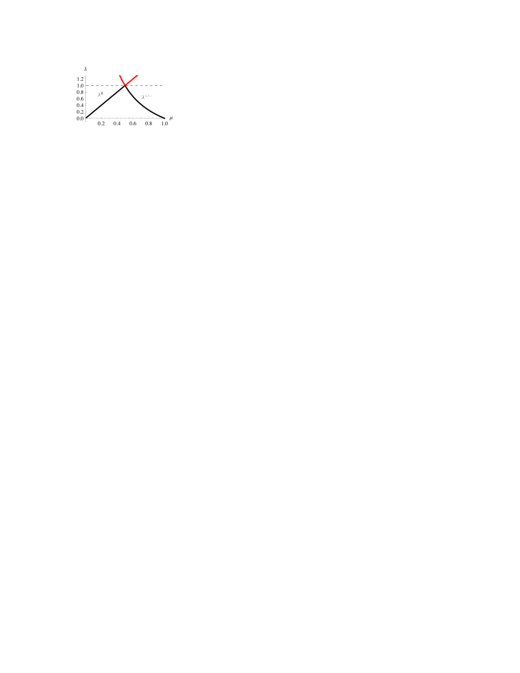
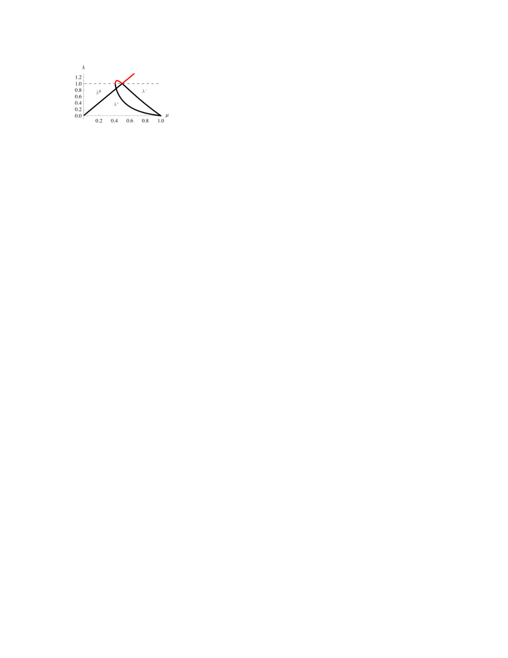
For $q>2$, $\kappa_{\infty}^{+}$ no longer intercepts the strong-coupling fixed-point line at $\kappa_{\infty}^{0}=0$, see Fig. 2, rendering the issue moot. The critical behavior with an infinite-order BKT-like transition is now described by analyzing the RG-flow near the branch point itself, as previously described [15, 24, 27, 19], moving the critical point to $\mu_{c}=\mu_{B}<\frac{1}{2}$ for $q>2$, where ${\cal D}_{q}\left(\mu_{B}\right)=0$ in Eq. (6) gives $\mu_{B}=2\left[q\sqrt{q-1}-2\left(q-1\right)\right]/\left(q-2\right)^{2}$.

We now study the effect of an external field for $\eta\to 1$ to analyze the behavior of the order parameter near the transition. In the limit $\eta\to 1$, i.e., $\theta\to 1$, and $\kappa\to\kappa_{\infty}$, Eqs. (3) provide the Jacobian matrix $\frac{\partial\left(\theta^{\prime},\kappa^{\prime}\right)}{\partial\left(\theta,\kappa\right)}$, which turns out to be upper-triangular, since $\frac{\partial\theta^{\prime}}{\partial\kappa}=0$ at $\theta=1$. Hence, the thermal exponent $y_{t}$ remains unaffected by the magnetic field. Accordingly, we obtain the magnetic exponent $y_{h}=\log_{2}\lambda_{h}$ with

when evaluated along $\kappa_{\infty}^{+}$ near $\mu_{c}=\frac{1}{2}$. As $\lambda_{h}$ is purely a function of $\kappa_{\infty}^{2}$, there are no odd correction terms for the exponent near $\mu_{c}$,

At $q=2$, we arrive at a more generic form, but merely by the fact that $\kappa_{\infty}^{+}$ now has its root-singularity:

Using the standard scaling relation [31] for the behavior of the order parameter near the transition,

we find $\beta=0$ for all $q<2$, while $\beta=\frac{1}{2}$ for $q=2$. The later result, predicting a 2nd-order transition with a mean-field-like exponent, has been obtained previously [26]. However, the former result suggests that the discontinuous percolation transitions found on various hyperbolic networks [6, 32, 14] is not an artifact of the particular percolation limit $q\to 1$ of the $q$-state Potts model but is maintained for all $q<2$. As soon as $q>2$ (now with $\mu_{c}=\mu_{B}$), $1-y_{h}$ remains finite while $y_{t}\to 0$ for $\mu\to\mu_{c}$ such that $\beta$ diverges and the transition becomes instantly infinite-order, as explained in Ref. [27].

Another perspective on these peculiar transitions is provided by the exponent [26]

for $\mu>\mu_{c}$, and $\Psi\equiv 1$ for $\mu<\mu_{c}$, that describes the divergence of the susceptibility with the system size,

not only near the transition but for all temperatures $0\leq\mu\leq 1$. For percolation, $\chi$ is related to the average size of the largest cluster, $\left\langle S(p)\right\rangle$, after a derivative in $q$. In Fig. 4, we plot $\Psi\left(\mu\right)$ in Eq. (15) for various $q$. The non-generic behavior of $y_{h}$ also manifests itself in $\Psi$: no branch of $\Psi$ ever exceeds unity, as could be generically expected, but rather $\Psi$ maintains a global extremum exactly of unit height for all $q\not=2$. Also Ref. [32] has found the same “delicate” behavior in $\Psi$ while studying the transformation of the transition from discontinuous to infinite-order for a one-parameter family of percolation models. The generic case can be observed, for instance, for the families of Ising models studied in Ref. [24] by applying an external field [33], where $y_{h}$ and hence $\Psi$ exhibit linear corrections near $\mu_{c}$ because the branch point singularity is outside the physical regime and $\Psi$ develops a maximum at an unphysical value $\Psi>1$, rendering the magnetization order parameter continuous at $\mu_{c}$.

While we found that the RG results for the couplings and $y_{t}$ of the $q$-state Potts are continuously connected to those of percolation at $q\to 1$, this is not true for $\Psi$ (i.e., $y_{h}$ or possibly other quantities that are affected by a $q$-derivate of the partition function). However, a direct comparison reveals that the Potts model at $q=1$ in Eq. (12) and the percolation result from Eq. (14) in Ref. [6] merely differ by a factor of 2 in their $2nd$-order correction near $\mu_{c}$. Their difference is more pronounced for larger $\mu$, of course. For example, $\Psi$ remains positive for all $\mu<1$ in percolation and only vanishes for zero bond-probability, $p=1-\mu=0$, suggesting that diverging clusters are always possible. In turn, $\Psi$ vanishes for non-trivial values of $\mu$ in the $q$-state Potts model, see Fig. 4, as is easily obtained from Eq. (11). While insignificant for $q<2$, this remains true, remarkably, at $q\geq 2$, which implies another potentially interesting transition in the behavior of $\chi$ at temperatures above criticality where fluctuations become independent of system size $N$, as shown in Fig. 5. There, we demonstrate the collapse of the data for $\chi$ when properly rescaled with system size $N$ according to Eq. (16). We observe a local minimum at $\mu_{c}$ which reaches a finite value on this scale for $q<2$ but appears to rapidly go to zero for all larger $q$ with increasing $N$. For $q\to 1$, a further factor of $q-1$ is required to converge to a thermodynamic limit. (Remember that $\chi$ at $q=1$ is not directly related to the percolation cluster size, which would require an additional derivative of $q$ in the partition function.) Most remarkable is the spike in $\chi$ at the point $\mu$ where $\Psi(\mu)$ becomes zero, see Fig. 4. Only above such temperature do fluctuations behave according to a high-temperature regime, independent of system size $N$. Such a transition from finite-size to diverging but subextensive fluctuations was absent, for instance, in the Ising model studied on any of the networks considered in Ref. [24].

To understand what makes these networks behave in such a non-generic way, let us consider the case of percolation on a binary tree, the most extreme hyperbolic network. Starting from the root of the tree at level $i=0$, the average number of sites at branching level $i>0$ that are connected in a single cluster with the root is $\left\langle n_{i+1}\right\rangle=2p\left\langle n_{i}\right\rangle$, hence, the average size of the rooted cluster at system size $N_{k}=2^{k+1}-1$ is $\left\langle S_{k}(p)\right\rangle=\sum_{i=0}^{k}\left\langle n_{i}\right\rangle=\left[(2p)^{k+1}-1\right]/\left(2p-1\right)$, or $\left\langle S(p)\right\rangle\sim N^{\Psi\left(p\right)}$ with $\Psi\left(p\right)=\log_{2}\left(2p\right)$ for $\frac{1}{2}<p<p_{c}=1$. Just like on any other hyperbolic network, there are diverging, yet sub-extensive, clusters well below $p_{c}$. (In fact, such diverging cluster emerge as soon as there are spanning clusters connecting the root to the perimeter of the tree, for $\frac{1}{2}<p<p_{c}$.) However, here we find linear corrections,

remembering that $\mu\hat{=}1-p$. We suggest that the relevant feature that distinguishes the networks with non-trivial explosive percolation transitions [28] with $p_{c}<1$ from the trivial cases with $p_{c}=1$, like this tree, is the interplay between a geometric backbone and the small-world hyperbolic links. For instance, adding lateral links turn the tree into a non-amenable graph with a non-trivial transition, studied in Refs. [18, 34]. Similarly, MK1 here, or the hyperbolic Hanoi networks in Ref. [14], become non-trivial by mixing geometric with hyperbolic structures. It is remarkable, that in Ref. [22] the tree-approximation for $\Psi\left(p\right)$ for percolation on a hyperbolic network, that is exact for $p<p_{l}$ but predicts a trivial transition at $p_{c}=1$ with linear corrections in $\Psi\left(p\right)$, breaks down above $p_{l}$ exactly where the geometric backbone begins to facilitate spanning clusters [17] and ultimately leads to a non-trivial explosive transition at $p_{c}<1$, again with quadratic corrections in $\Psi\left(p\right)$ [14]. While renormalization group calculations provide these exact results, it will likely require more detailed numerical simulations or better models to elucidate the role of geometry in the dynamics of cluster formation that lead to such corrections.

Finally, we speculate on the origin of the singularity of the $q$-state Potts model for $q\to 2$. What distinguishes the $q\geq 2$ case from that for $q<2$ is the nature of the $Z_{q}$-symmetry [29]. While for $q<2$ (and, correspondingly, for percolation) it is sufficient to merge two clusters by merely adding a link, for $q\geq 2$ (i.e., for the Ising spin model or other multi-state degrees of freedom) two cluster only merge when both share the same orientation. Apparently, the analytic continuation in $q$ delimits these two distinct cluster-growth processes via a singularity at $q\to 2$.

We like to thank T. Nogawa and T. Hasegawa for fruitful discussions. This work was supported by NSF (DMR #1207431 & IOS #1208126) and James S. McDonnell Foundation (#220020321).

References

- [1] M. Barthelemy, EPL (Europhysics Letters) 63, 915 (2003).
- [2] S. Boccaletti, V. Latora, Y. Moreno, M. Chavez, and D.-U. Hwang, Phys. Rep. 424, 175 (2006).
- [3] S. N. Dorogovtsev, A. V. Goltsev, and J. F. F. Mendes, Rev. Mod. Phys. 80, 1275 (2008).
- [4] D. J. Watts and S. H. Strogatz, Nature 393, 440 (1998).
- [5] A.-L. Barabasi and R. Albert, Science 286, 509 (1999).
- [6] S. Boettcher, V. Singh, and R. M. Ziff, Nature Communications 3, 787 (2012).
- [7] D. Achlioptas, R. M. D’Souza, and J. Spencer, Science 323, 1453 (2009).
- [8] R. A. da Costa, S. N. Dorogovtsev, A. V. Goltsev, and J. F. F. Mendes, Phys. Rev. Lett. 105, 255701 (2010).
- [9] P. Grassberger, C. Christensen, G. Bizhani, S.-W. Son, and M. Paczuski, Phys. Rev. Lett. 106, 225701 (2011).
- [10] H. K. Lee, B. J. Kim, and H. Park, Phys. Rev. E 84, 020101 (2011).
- [11] O. Riordan and L. Warnke, Science 333, 322 (2011).
- [12] N. Bastas, P. Giazitzidis, M. Maragakis, and K. Kosmidis, Physica A: Statistical Mechanics and its Applications 407, 54 (2014).
- [13] N. A. M. Araújo, P. Grassberger, B. Kahng, K. J. Schrenk, and R. M. Ziff, (arXiv:1404.5325).
- [14] V. Singh and S. Boettcher, Physical Review E 90, 012117 (2014).
- [15] M. Hinczewski and A. N. Berker, Phys. Rev. E 73, 066126 (2006).
- [16] S. Boettcher, B. Gonçalves, and H. Guclu, J. Phys. A: Math. Theor. 41, 252001 (2008).
- [17] S. Boettcher, J. L. Cook, and R. M. Ziff, Phys. Rev. E 80, 041115 (2009).
- [18] T. Nogawa and T. Hasegawa, J. Phys. A: Math. Theor. 42, 145001 (2009).
- [19] T. Nogawa, T. Hasegawa, and K. Nemoto, Phys. Rev. Lett. 108, 255703 (2012).
- [20] A. N. Berker, M. Hinczewski, and R. R. Netz, Phys. Rev. E 80, 041118 (2009).
- [21] P. Minnhagen and S. K. Baek, Phys. Rev. E 82, 011113 (2010).
- [22] T. Hasegawa and T. Nogawa, Phys. Rev. E 87, 032810 (2013).
- [23] M. Bauer, S. Coulomb, and S. N. Dorogovtsev, Phys. Rev. Lett. 94, 200602 (2005).
- [24] S. Boettcher and C. T. Brunson, Phys. Rev. E 83, 021103 (2011).
- [25] S. K. Baek, H. Mäkelä, P. Minnhagen, and B. J. Kim, Phys. Rev. E 84, 032103 (2011).
- [26] T. Nogawa, T. Hasegawa, and K. Nemoto, Phys. Rev. E 86, 030102 (2012).
- [27] S. Boettcher and C. T. Brunson, (arXiv:1209.3447).
- [28] Y. S. Cho and B. Kahng, (arXiv:1404.4470).
- [29] F. Y. Wu, Reviews of Modern Physics 54, 235 (1982).
- [30] M. Plischke and B. Bergersen, Equilibrium Statistical Physics, 2nd edition (World Scientifc, Singapore, 1994).
- [31] R. K. Pathria, Statistical Mechanics, 2nd Ed. (Butterworth-Heinemann, 1996).
- [32] T. Nogawa and T. Hasegawa, Phys. Rev. E 89, 042803 (2014).
- [33] C. T. Brunson and S. Boettcher, (in preparation).
- [34] T. Hasegawa, T. Nogawa, and K. Nemoto, EuroPhys. Lett. 104, 16006 (2013).