跳到论文正文
W Papers独立论文阅读器 arXiv:1408.0412 论文正文 计算阅读时间 · 0%
引用这篇论文根据当前论文元数据生成,正式投稿前建议核对。


License: arXiv.org perpetual non-exclusive license
arXiv:1408.0412v2 [math.ST] 05 Jun 2015

Asymptotic Properties of the Empirical Spatial Extremogram

Yongbum Cho and Richard A. Davis
Department of Statistics, Columbia University
Souvik Ghosh
LinkedIn Corporation

ABSTRACT. The extremogram is a useful tool for measuring extremal dependence and checking model adequacy in a time series. We define the extremogram in the spatial domain when the data is observed on a lattice or at locations distributed as a Poisson point process in dd-dimensional space. We establish a central limit theorem for the empirical spatial extremogram. We show these conditions are applicable for max-moving average processes and Brown-Resnick processes and illustrate the empirical extremogram’s performance via simulation. We also demonstrate its practical use with a data set related to rainfall in a region in Florida.

Keywords: extremal dependence; extremogram; max moving average; max stable process; spatial dependence

1 Introduction

Extreme events can affect our lives in many dimensions. Events like large swings in financial markets or extreme weather conditions such as floods and hurricanes can cause large financial/property losses and numerous casualties. Extreme events often appear to cluster and that has resulted in a growing interest in measuring extremal dependence in many areas including finance, insurance, and atmospheric science.

Extremal dependence between two random vectors XX and YY can be viewed as the probability that XX is extreme given YY belongs to an extreme set. The extremogram, proposed by Davis and Mikosch (2009), is a versatile tool for assessing extremal dependence in a stationary time series. The extremogram has two main features:

  • •

    It can be viewed as the extreme-value analog of the autocorrelation function of a stationary time series, i.e., extremal dependence is expressed as a function of lag.

  • •

    It allows for measuring dependence between random variables belonging in a large variety of extremal sets. Depending on choices of sets, many of the commonly used extremal dependence measures - right tail dependence, left tail dependence, or dependence among large absolute values - can be treated as a special case of the extremogram. The flexibility coming from arbitrary choices of extreme sets have made it especially well suited for time series applications such as high-frequency FX rates (Davis and Mikosch (2009)), cross-sectional stock indices (Davis et al. (2012)), and CDS spreads (Cont and Kan (2011)).

In this paper, we will define the notion of the extremogram for random fields defined on ℝd\mathbb{R}^{d} for some d>1d>1 and investigate the asymptotic properties of its corresponding empirical estimate. Let {Xs,s∈ℝd}\{X_{s},s\in\mathbb{R}^{d}\} be a stationary ℝk\mathbb{R}^{k}-valued random field. For measurable sets A,B⊂ℝkA,B\subset\mathbb{R}^{k} bounded away from 0, we define the spatial extremogram as

ρA​B​(h)=limx→∞P⁡(Xh∈x​B|X0∈x​A),h∈ℝd,\displaystyle\rho_{AB}(h)=\lim_{x\rightarrow\infty}P(X_{h}\in xB|X_{\textbf{0}}\in xA),\quad h\in\mathbb{R}^{d}, (1.1)

provided the limit exists. We call (1.1) the spatial extremogram to emphasize that it is for a random field in ℝd.\mathbb{R}^{d}. If one takes A=B=(1,∞)A=B=(1,\infty) in the k=1k=1 case, then we recover the tail dependence coefficient between XhX_{h} and X0.X_{\textbf{0}}. For light tailed time series, such as stationary Gaussian processes, ρA​B​(h)=0\rho_{AB}(h)=0 for h≠0h\neq\textbf{0} in which case there is no extremal dependence. However, for heavy tailed processes in either time or space, ρA​B​(h)\rho_{AB}(h) is often non-zero for many lags h≠0h\neq\textbf{0} and for most choices of sets AA and BB bounded away from the origin.

We will consider estimates of ρA​B​(h)\rho_{AB}(h) under two different sampling scenarios. In the first, observations are taken on the lattice ℤd\mathbb{Z}^{d}. Analogous to Davis and Mikosch (2009), we define the empirical spatial extremogram (ESE) as

ρ^A​B,m​(h)=∑s,t∈Λn,s−t=hI{am−1​Xs∈A,am−1​Xt∈B}/n⁡(h)∑s∈ΛnI{am−1Xs∈A}/#Λn,\hat{\rho}_{AB{,m}}(h)=\frac{\sum_{s,t\in\Lambda_{n},s-t=h}I_{\{a_{m}^{-1}X_{s}\in A,a_{m}^{-1}X_{t}\in B\}}/n(h)}{\sum_{s\in\Lambda_{n}}I_{\{a_{m}^{-1}X_{s}\in A\}}/{\#\Lambda_{n}}}, (1.2)

where

  • •

    Λn={1,2,.…,n}d\Lambda_{n}=\{1,2,.\ldots,n\}^{d} is the dd-dimensional cube with side length nn,

  • •

    h∈ℤdh\in\mathbb{Z}^{d} are observed lags in Λn\Lambda_{n},

  • •

    m=mnm=m_{n} is an increasing sequence satisfying m→∞m\to\infty and m/n→0m/n\rightarrow 0 as n→∞n\to\infty,

  • •

    ama_{m} is a sequence such that P⁡(|X|>am)∼m−1P(|X|>a_{m})\sim m^{-1},

  • •

    n⁡(h)n(h) is the number of pairs in Λn\Lambda_{n} with lag hh, and

  • •

    #​Λn\#\Lambda_{n} is the cardinality of Λn\Lambda_{n}.

In the second case, the data are assumed to come from a stationary random field Xs,X_{s}, where the locations {s1,…,sN}\{s_{1},...,s_{N}\} are assumed to be points of a homogeneous Poisson point process on Sn⊂ℝdS_{n}\subset\mathbb{R}^{d}. We define the empirical spatial extremogram as a kernel estimator of ρA​B​(h)\rho_{AB}(h), in the spirit of the estimate of autocorrelation in space (see Li et al. (2008)). Under suitable growth conditions on SnS_{n} and restrictions on the kernel function, we show that the weighted estimator of ρA​B​(h)\rho_{AB}(h) is consistent and asymptotically normal.

The organization of the paper is as follows: In Section 2, we present the asymptotic properties of the ESE for both cases described above. Section 3 provides examples illustrating the results of Section 2 together with a simulation study demonstrating the performance of the ESE. In Section 4, the spatial extremogram is applied to a spatial rainfall data set in Florida. The proofs of all the results are in the Appendix.

2 Asymptotics of the ESE

2.1 Definitions and notation

Let {Xs,s∈I}\{X_{s},s\in I\} be a kk-dimensional strictly stationary random process where II is either ℝd\mathbb{R}^{d} or ℤd\mathbb{Z}^{d}. For H={h1,…,ht}⊂IH=\{h_{1},\ldots,h_{t}\}\subset I, we use XHX_{H} to denote (Xh1,…,Xht)(X_{h_{1}},\ldots,X_{h_{t}}). The random field is said to be regularly varying with index α>0\alpha>0 if for any H,H, the radial part ‖XH‖\|X_{H}\| satisfies for all y>0y>0

(C1) P⁡(‖XH‖>y​x)P⁡(‖XH‖>x)→y−α​ as ​x→∞,\displaystyle\qquad\qquad\qquad\qquad\qquad\qquad\qquad\frac{P\big(\|X_{H}\|>yx\big)}{P\big(\|X_{H}\|>x\big)}\rightarrow y^{-\alpha}\;\mbox{ as }x\to\infty,

and the angular part XH‖XH‖\frac{X_{H}}{\|X_{H}\|} is asymptotically independent of the radial part ‖XH‖\|X_{H}\| for large values of ‖XH‖\|X_{H}\|, i.e., there exists a random vector ΘH∈𝕊t​k−1\Theta_{H}\in\mathbb{S}^{tk-1}, the unit sphere in ℝt​k\mathbb{R}^{tk} with respect to ∥⋅∥\|\cdot\|, such that

(C2) P(XH‖XH‖∈⋅|∥XH∥>x)→𝑤P(ΘH∈⋅) as x→∞,\displaystyle\qquad\qquad\qquad\qquad\qquad P\left(\frac{X_{H}}{\|X_{H}\|}\in\cdot\Big|\|X_{H}\|>x\right)\xrightarrow{w}P\left(\Theta_{H}\in\cdot\right)\;\mbox{ as }x\to\infty,

where →𝑤\xrightarrow{w} denotes weak convergence. The distribution of P(ΘH∈⋅)P\left(\Theta_{H}\in\cdot\right) is called the spectral measure of XHX_{H}.

An equivalent definition of regular variation is given as follows. There exists a sequence an→∞,α>0a_{n}\rightarrow\infty,\alpha>0 and a family of non-null Radon measures (μH)(\mu_{H}) on the Borel σ\sigma-field of ℝ¯t​k∖{0}\bar{\mathbb{R}}^{tk}\setminus\{\textbf{0}\} such that nP(an−1XH∈⋅)→𝑣μH(⋅)nP(a_{n}^{-1}X_{H}\in\cdot)\xrightarrow{v}\mu_{H}(\cdot) for t≥1t\geq 1, where the limiting measure satisfies μH(y⋅)=y−αμH(⋅)\mu_{H}(y\cdot)=y^{-\alpha}\mu_{H}(\cdot) for y>0y>0 . Here, →𝑣\xrightarrow{v} denotes vague convergence. Under the regularly varying assumption, one can show that (1.1) is well defined. See Section 6.1 of Resnick (2006) for more details.

2.2 Random fields on a lattice

Let {Xs,s∈ℤd}\{X_{s},s\in\mathbb{Z}^{d}\} be a strictly stationary random field and suppose we have observations {Xs,s∈Λn={1,…,n}d}\{X_{s},s\in\Lambda_{n}=\{1,...,n\}^{d}\}. Let d⁡(⋅,⋅)d(\cdot,\cdot) be a metric on ℤd\mathbb{Z}^{d}. We denote the α\alpha-mixing coefficient by

αj,k(r)=sup{α(σ(Xs,s∈S),σ(Xs,s∈T)):S,T⊂ℤd,#S≤j,#T≤k,d(S,T)≥r},\alpha_{j,k}(r)=\sup\big\{\alpha\big(\sigma(X_{s},s\in S),\sigma(X_{s},s\in T)\big):S,T\subset\mathbb{Z}^{d},{\#S\leq j,\#T\leq k},d(S,T)\geq r\big\},

where for any two σ\sigma-fields 𝒜\mathcal{A} and ℬ\mathcal{B}, α(𝒜,ℬ)=sup{|P(A∩B)−P(A)P(B)|:A∈𝒜,B∈ℬ}\alpha(\mathcal{A},\mathcal{B})=\sup\{|P(A\cap B)-P(A)P(B)|:A\in\mathcal{A},B\in\mathcal{B}\} and for any S,T⊂ℤdS,T\subset\mathbb{Z}^{d}, d(S,T)=inf{d(s,t):s∈S,t∈T}d(S,T)=\inf\{d(s,t):s\in S,t\in T\}.

In order to study asymptotic properties of (1.2), we impose regularly varying and certain mixing conditions on the random field. In particular, we use the big/small block argument: the side length of big blocks, mnm_{n}, and the distance between big blocks, rnr_{n}, have to be coordinated in the right fashion. To be precise, we assume the following conditions.

(M1) Let BγB_{\gamma} be the ball of radius γ{\gamma} centered at 0, i.e., Bγ={s∈ℤd:d⁡(0,s)≤γ},B_{\gamma}=\{s\in\mathbb{Z}^{d}:d(\textbf{0},s)\leq{\gamma}\}, and set c=#​Bγc=\#B_{\gamma}. For a fixed γ\gamma, assume that there exist mn,rn→∞m_{n},r_{n}\rightarrow\infty with mn2+2​d/nd→0{m_{n}^{2+2d}}/{n^{d}}\rightarrow 0, rnd/mn→0{r_{n}^{d}}/{m_{n}}\rightarrow 0 such that

limk→∞lim supn→∞mn​∑l∈ℤd,k<d⁡(0,l)≤rnP⁡(maxs∈Bγ⁡|Xs|>ϵ​am,maxs′∈Bγ+l⁡|Xs′|>ϵ​am)=0for∀ϵ>0,\displaystyle\displaystyle\lim_{k\rightarrow\infty}\limsup_{n\rightarrow\infty}m_{n}\sum_{l\in\mathbb{Z}^{d},k<d(\textbf{0},l)\leq r_{n}}P\left(\max_{{s}\in B_{\gamma}}|X_{{s}}|>{\epsilon a_{m}},\max_{{s}^{\prime}\in B_{\gamma}+l}|X_{{s}^{\prime}}|>{\epsilon a_{m}}\right)=0\quad\text{for}\quad\forall\epsilon>0, (2.1)
limn→∞mn​∑l∈ℤd,rn<d⁡(0,l)αc,c​(d⁡(0,l))=0,\displaystyle\lim_{n\rightarrow\infty}m_{n}\sum_{l\in\mathbb{Z}^{d},r_{n}<d(\textbf{0},l)}\alpha_{c,c}(d(\textbf{0},l))=0, (2.2)
∑l∈ℤdαj1,j2​(d⁡(0,l))<∞for2​c≤j1+j2≤4​c,\displaystyle\sum_{l\in\mathbb{Z}^{d}}\alpha_{j_{1},j_{2}}(d(\textbf{0},l))<\infty\quad\text{for}\quad 2c\leq j_{1}+j_{2}\leq 4c, (2.3)
limn→∞nd/2​mn1/2​αc,c​nd​(mn)=0,\displaystyle\lim_{n\rightarrow\infty}n^{d/2}m_{n}^{1/2}\alpha_{c,cn^{d}}(m_{n})=0, (2.4)

where ama_{m} satisfies P⁡(|X|>am)∼1m.P(|X|>a_{m})\sim\frac{1}{m}.

Condition (2.1) restricts the joint distributions for exceedance as two sets of points become far apart. Conditions (2.2) - (2.4) impose restrictions on the decaying rate of the mixing functions together with the level of the threshold specified by mnm_{n}. These conditions are similar to those in Bolthausen (1982) and Davis and Mikosch (2009).

As in Davis and Mikosch (2009), the ESE ρ^A​B,m​(h)\hat{\rho}_{AB,m}(h) is centered by the Pre-Asymptotic (PA) extremogram

ρA​B,m​(h)=τA​B,m​(h)pm​(A),\displaystyle{\rho}_{AB,m}(h)=\frac{{\tau}_{AB,m}(h)}{{p}_{m}(A)}, (2.5)

where τA​B,m​(h)=mn​P​(X0∈am​A,Xh∈am​B){\tau}_{AB,m}(h)=m_{n}P(X_{\textbf{0}}\in a_{m}A,X_{h}\in a_{m}B) and pm​(A)=mn​P​(X0∈am​A)p_{m}(A)=m_{n}P(X_{\textbf{0}}\in a_{m}A). Notice that (2.5) is the ratio of the expected value of the numerator and denominator in (1.2).

Theorem 2.1.

Suppose a strictly stationary regularly varying random field {Xs,s∈ℤd}\{X_{\textbf{s}},s\in\mathbb{Z}^{d}\} with index α>0\alpha>0 is observed on Λn={1,…,n}d\Lambda_{n}=\{1,...,n\}^{d}. For any finite set of non-zero lags HH in ℤd\mathbb{Z}^{d}, assume (M1), where Bγ⊇HB_{\gamma}\supseteq H for some γ{\gamma}. Then

ndmn​[ρ^A​B,m​(h)−ρA​B,m​(h)]h∈H→𝑑N⁡(0,Σ),\sqrt{\frac{n^{d}}{m_{n}}}\Big[\hat{\rho}_{AB,m}(h)-\rho_{AB,m}(h)\Big]_{h\in H}\xrightarrow{d}N(\textbf{0},\Sigma),

where the matrix Σ\Sigma in normal distribution is specified in Appendix A.

We present the proof of Theorem 2.1 in Appendix A. Examples of heavy-tailed processes satisfying (M1) are presented in Section 3.

Remark 1.

In Theorem 2.1, the pre-asymptotic extremogram ρA​B,m​(h)\rho_{AB,m}(h) is replaced by the extremogram ρA​B​(h)\rho_{AB}(h) if

limn→∞ndmn​|ρA​B,m​(h)−ρA​B​(h)|=0,f​o​rh∈H.\displaystyle\lim_{n\rightarrow\infty}\sqrt{\frac{n^{d}}{m_{n}}}|\rho_{AB,m}(h)-\rho_{AB}(h)|=0,\;\quad for\quad\;h\in H. (2.6)

2.3 Random fields on ℝd\mathbb{R}^{d}

Now consider the case of a random field defined on ℝd\mathbb{R}^{d} and the sampling locations are given by points of a Poisson process. In this case, we adopt the ideas from Karr (1986) and Li et al. (2008) and use a kernel estimate of the extremogram. For convenience, we restrict our attention to ℝ2\mathbb{R}^{2}. The extension to ℝd​(d>1)\mathbb{R}^{d}(d>1) is straightforward, but notationally more complex.

Let {Xs,s∈ℝ2}\{X_{s},s\in\mathbb{R}^{2}\} be a stationary regularly varying random field with index α>0\alpha>0. Suppose NN is a homogeneous 2-dimensional Poisson process with intensity parameter ν\nu and is independent of XX. Define N(2)​(d​s1,d​s2)=N⁡(d​s1)​N​(d​s2)​I​(s1≠s2)N^{(2)}(ds_{1},ds_{2})=N(ds_{1})N(ds_{2})I(s_{1}\neq s_{2}). Now consider a sequence of compact and convex sets Sn⊂ℝ2S_{n}\subset\mathbb{R}^{2} with Lebesgue measure |Sn|→∞|S_{n}|\rightarrow\infty as n→∞n\rightarrow\infty. Assume that for each y∈ℝ2y\in\mathbb{R}^{2}

limn→∞|Sn∩(Sn−y)||Sn|=1,\displaystyle\lim_{n\rightarrow\infty}\frac{|S_{n}\cap(S_{n}-y)|}{|S_{n}|}=1, (2.7)

where Sn−y={x−y:x∈Sn}S_{n}-y=\{x-y:x\in S_{n}\},

|Sn|=O⁡(n2),|∂Sn|=O⁡(n),\displaystyle|S_{n}|=O(n^{2}),\qquad|\partial S_{n}|=O(n), (2.8)

and ∂Sn\partial S_{n} denotes the boundary of SnS_{n}.

The spatial extremogram in (1.1) is estimated by ρ^A​B,m​(h)=τ^A​B,m​(h)/p^m​(A),\displaystyle\hat{\rho}_{AB,m}(h)={\hat{\tau}_{AB,m}(h)}/{\hat{p}_{m}(A)}, where

p^m​(A)=mnν​|Sn|​∫SnI⁡(Xs1am∈A)​N​(d​s1),\displaystyle\hat{p}_{m}(A)=\frac{m_{n}}{\nu|S_{n}|}\int_{S_{n}}I\left(\frac{X_{s_{1}}}{a_{m}}\in A\right)N(ds_{1}), (2.9)
τ^A​B,m​(h)=mnν2​1|Sn|​∫Sn∫Snwn​(h+s1−s2)​I​(Xs1am∈A)​I​(Xs2am∈B)​N(2)​(d​s1,d​s2).\displaystyle\hat{\tau}_{AB,m}(h)=\frac{m_{n}}{\nu^{2}}\frac{1}{|S_{n}|}\int_{S_{n}}\int_{S_{n}}w_{n}(h+s_{1}-s_{2})\;I\left(\frac{X_{s_{1}}}{a_{m}}\in A\right)I\left(\frac{X_{s_{2}}}{a_{m}}\in B\right)N^{(2)}(ds_{1},ds_{2}). (2.10)

Here wn​(⋅)=1λn2​w​(⋅λn)w_{n}(\cdot)=\frac{1}{\lambda_{n}^{2}}w(\frac{\cdot}{\lambda_{n}}) is a sequence of weight functions, where w⁡(⋅)w(\cdot) on ℝ2\mathbb{R}^{2} is a positive, bounded, isotropic probability density function and λn\lambda_{n} is the bandwidth satisfying λn→0\lambda_{n}\rightarrow 0 and λn2​|Sn|→∞.\lambda_{n}^{2}|S_{n}|\rightarrow\infty. To establish a central limit theorem for ρ^A​B,m​(h)\hat{\rho}_{AB,m}(h), we derive asymptotics of the denominator p^m​(A){\hat{p}_{m}(A)} and numerator τ^A​B,m​(h){\hat{\tau}_{AB,m}(h)}. In order to show consistency of p^m​(A){\hat{p}_{m}(A)}, we assume the following conditions, which are the non-lattice analogs of (2.1) and (2.2).

(M2) There exist an increasing sequence mnm_{n} and rnr_{n} with mn=o⁡(n)m_{n}=o(n) and rn2=o⁡(mn)r_{n}^{2}=o(m_{n}) such that

limk→∞lim supn→∞∫B⁡[k,rn]mn​P​(|Xy|>ϵ​am,|X0|>ϵ​am)​𝑑y=0for∀ϵ>0,\displaystyle\lim_{k\rightarrow\infty}\limsup_{n\rightarrow\infty}\int_{B[k,r_{n}]}m_{n}P(|X_{y}|>\epsilon a_{m},|X_{\textbf{0}}|>\epsilon a_{m})dy=0\quad\text{for}\quad\forall\epsilon>0, (2.11)
limn→∞∫ℝ2∖B[0,rn)mnα1,1(y)dy=0,\displaystyle\lim_{n\rightarrow\infty}\int_{\mathbb{R}^{2}\setminus B[{0},r_{n})}m_{n}\alpha_{1,1}(y)dy=0, (2.12)
∫ℝ2τA​A​(y)​𝑑y<∞,\displaystyle\int_{\mathbb{R}^{2}}\tau_{AA}(y)dy<\infty, (2.13)

where B[a,b)={s:a≤d(0,s)<b,s∈ℝ2}B[a,b)=\{s:a\leq d(\textbf{0},s)<b,s\in\mathbb{R}^{2}\} and τA​A​(y)=limn→∞τA​A,m​(y)\displaystyle{\tau}_{AA}(y)=\lim_{n\rightarrow\infty}{\tau}_{AA,m}(y).

For a central limit theorem for τ^A​B,m​(h){\hat{\tau}_{AB,m}(h)}, the following conditions are required.

(M3) Consider a cube Bn⊂SnB_{n}\subset S_{n} with |Bn|=O⁡(n2​a)|B_{n}|=O(n^{2a}) and |∂Bn|=O⁡(na)|\partial B_{n}|=O(n^{a}) for 0<a<1.0<a<1. Assume that there exist an increasing sequence mnm_{n} with mn=o⁡(na)m_{n}=o(n^{a}) and λn2​mn→0\lambda_{n}^{2}m_{n}\rightarrow 0 such that

supnE⁡{|Bn|​λn2mn​|τ^A​B,m​(h:Bn)−E​τ^A​B,m​(h:Bn)|2+δ}≤Cδ,δ>0,Cδ<∞,\displaystyle\displaystyle\sup_{n}E\left\{\sqrt{\frac{|B_{n}|\lambda_{n}^{2}}{m_{n}}}\big|\hat{\tau}_{AB,m}(h:B_{n})-E\hat{\tau}_{AB,m}(h:B_{n})\big|^{2+\delta}\right\}\leq C_{\delta},\quad\delta>0,\;C_{\delta}<\infty, (2.14)

where τ^A​B,m​(h:Bn)\hat{\tau}_{AB,m}(h:B_{n}) is the quantity (2.10) with SnS_{n} replaced by BnB_{n} on the right-hand side. Further assume

∫ℝ2τA​B​(y)​𝑑y<∞,∫ℝ2α2,2​(d⁡(0,y))​𝑑y<∞,\displaystyle\int_{\mathbb{R}^{2}}\tau_{AB}(y)dy<\infty,\;\;\int_{\mathbb{R}^{2}}\alpha_{2,2}(d(\textbf{0},y))dy<\infty, (2.15)

and

suplαl,l​(h)l2=O⁡(h−ϵ)f​o​r​s​o​m​e​ϵ>0.\displaystyle\displaystyle\sup_{l}\frac{\alpha_{l,l}(h)}{l^{2}}=O(h^{-\epsilon})\quad for\;some\;\epsilon>0. (2.16)

Lastly, the proof requires some smoothness of the random field.

Definition 2.2.

A stationary regularly varying random field {Xs,s∈ℝd}\{X_{s},s\in\mathbb{R}^{d}\} satisfies a local uniform negligibility condition (LUNC) if for an increasing sequence ana_{n} satisfying P⁡(|X|>an)∼1nP(|X|>a_{n})\sim\frac{1}{n} and for all ϵ,δ>0\epsilon,\delta>0, there exists δ′>0\delta^{\prime}>0 such that

lim supnn​P​(sup‖s‖<δ′|Xs−X0|an>δ)<ϵ.\displaystyle\limsup_{n}nP\left(\sup_{||s||<\delta^{\prime}}\frac{|X_{s}-X_{\textbf{0}}|}{a_{n}}>\delta\right)<\epsilon. (2.17)
Theorem 2.3.

Let {Xs,s∈ℝ2}\{X_{s},s\in\mathbb{R}^{2}\} be a stationary regularly varying random field with index α>0\alpha>0 satisfying LUNC. Assume NN is a homogeneous 2-dimensional Poisson process with intensity parameter ν\nu and is independent of XX. Consider a sequence of compact and convex sets Sn⊂ℝ2S_{n}\subset\mathbb{R}^{2} satisfying |Sn|→∞|S_{n}|\rightarrow\infty as n→∞n\rightarrow\infty. Assume conditions (M2) and (M3). Then for any finite set of non-zero lags HH in ℝ2\mathbb{R}^{2},

|Sn|​λn2mn​[ρ^A​B,m​(h)−ρA​B,m​(h)]h∈H→N⁡(0,Σ),\displaystyle\sqrt{\frac{|S_{n}|\lambda_{n}^{2}}{m_{n}}}\left[\hat{\rho}_{AB,m}(h)-{\rho}_{AB,m}(h)\right]_{h\in H}\rightarrow N(\textbf{0},\Sigma), (2.18)

where the matrix Σ\Sigma is specified in the proof of Theorem 2.1 in Appendix A.

We present the proof of Theorem 2.3 in Appendix B. As in Remark 1, ρA​B,m​(h){\rho}_{AB,m}(h) can be replaced by ρA​B​(h){\rho}_{AB}(h) if ρA​B,m​(h){\rho}_{AB,m}(h) converges fast enough.

Remark 2.

In (2.18), ρA​B,m​(h){\rho}_{AB,m}(h) can be replaced by ρA​B​(h){\rho}_{AB}(h) if

limn→∞|Sn|​λn2mn​|ρA​B,m​(h)−ρA​B​(h)|=0f​o​r​h∈H.\displaystyle\lim_{n\rightarrow\infty}\sqrt{\frac{|S_{n}|\lambda_{n}^{2}}{m_{n}}}|{\rho}_{AB,m}(h)-{\rho}_{AB}(h)|=0\qquad for\;h\in H. (2.19)

3 Examples

Here we provide two max-stable processes to illustrate the results of Section 2. For background on max-stable processes, see de Haan (1984) and de Haan and Ferreira (2006). In order to check conditions, we need the result from Dombry and Eyi-Minko (2012).

Proposition 3.1 (Dombry and Eyi-Minko (2012)).

Suppose {Xs,s∈S}\{X_{s},s\in S\} is a max-stable random field with unit Fréchet marginals. If S1S_{1} and S2S_{2} are finite or countable disjoint closed subsets of SS, and 𝒮1\mathcal{S}_{1} and 𝒮2\mathcal{S}_{2} are the respective σ\sigma-fields generated by each set, then

β⁡(𝒮1,𝒮2)≤4​∑s1∈S1∑s2∈S2ρ(1,∞)​(1,∞)​(‖s1−s2‖)\displaystyle\displaystyle\beta(\mathcal{S}_{1},\mathcal{S}_{2})\leq 4\sum_{s_{1}\in S_{1}}\sum_{s_{2}\in S_{2}}{\color[rgb]{0,0,0}\rho_{(1,\infty)(1,\infty)}(||s_{1}-s_{2}||)} (3.1)

where β⁡(⋅,⋅)\beta(\cdot,\cdot) is the β\beta-mixing coefficient. We refer to Lemma 2 in Davis et al. (2013).

Notice that (3.1) provides the upper bound for α\alpha-mixing coefficient since 2​α​(𝒮1,𝒮2)≤β⁡(𝒮1,𝒮2).2\alpha(\mathcal{S}_{1},\mathcal{S}_{2})\leq\beta(\mathcal{S}_{1},\mathcal{S}_{2}). See Bradley (1993).

3.1 Max Moving Average (MMA)

Let {Zs,s∈ℤ2}\{Z_{s},s\in\mathbb{Z}^{2}\} be an iid sequence of unit Fréchet random variables. The max-moving average (MMA) process is defined by

Xt=maxs∈ℤ2⁡w⁡(s)​Zt−s,\displaystyle X_{t}=\max_{s\in\mathbb{Z}^{2}}w(s)Z_{t-s}, (3.2)

where w⁡(s)>0​and​∑s∈ℤ2w⁡(s)<∞w(s)>0\;\text{and}\;\sum_{s\in\mathbb{Z}^{2}}w(s)<\infty. Note that the summability of w⁡(⋅)w(\cdot) implies the process is well defined. Also, notice that am=O⁡(m)a_{m}=O(m) since marginal distributions are Fréchet. Consider the Euclidean metric d⁡(⋅,⋅)d(\cdot,\cdot) and write ‖l‖=d⁡(0,l)||l||=d(\textbf{0},l) for notational convenience. With w⁡(s)=I⁡(‖s‖≤1)w(s)=I(||s||\leq 1), the process (3.2) becomes the MMA(1): Xt=max‖s‖≤1⁡Zt−s\displaystyle X_{t}=\max_{||s||\leq 1}Z_{t-s}. Using A=B=(1,∞)A=B=(1,\infty), the extremogram for the MMA(1) is then

ρA​B​(h)=limn→∞P⁡(Xh>amn|X0>amn)={1,if‖h‖=0,2/5,if‖h‖=1,2,1/5,if‖h‖=2,0,if‖h‖>2.\rho_{AB}(h)=\lim_{n\rightarrow\infty}P(X_{h}>a_{m_{n}}|X_{\textbf{0}}>a_{m_{n}})=\left\{\begin{array}[]{rll}1,&\mbox{if}&||h||=0,\\ 2/5,&\mbox{if}&||h||=1,\sqrt{2},\\ 1/5,&\mbox{if}&||h||=2,\\ 0,&\mbox{if}&||h||>2.\end{array}\right. (3.3)

Since the process is 2-dependent, conditions for Theorem 2.1 are easily checked.

Figure 1 (left) shows ρA​B​(h)\rho_{AB}(h) and ρ^A​B,m​(h)\hat{\rho}_{AB,m}(h) from a realization of MMA(1) generated by rmaxstab in the SpatialExtremes package11 1 http://cran.r-project.org/web/packages/SpatialExtremes/SpatialExtremes.pdf in R. We use 1600 points (Λn={1,…,40}2∈ℤ2\Lambda_{n}=\{1,...,40\}^{2}\in\mathbb{Z}^{2}) and set A=B=(1,∞)A=B=(1,\infty) and am=a_{m}= .97 quantile of the process. In the figure, the dots and the bars correspond to ρA​B​(h){\rho}_{AB}(h) and ρ^A​B,m​(h)\hat{\rho}_{AB,m}(h) for observed distances in the sample. The dashed line corresponds to 0.03(=1−0.97)0.03\;(=1-0.97) and two horizontal lines are 95% random permutation confidence bands to check the existence of extremal dependence (see Davis et al. (2012)). The bands suggest ρ(1,∞)​(1,∞),m​(h)=0{\rho}_{(1,\infty)(1,\infty),m}(h)=0 for h>2h>2, which is consistent with (3.3).

Figure 1: ρA​A​(h)\rho_{AA}(h) and ρ^A​A,m​(h)\hat{\rho}_{AA,m}(h), where A=(1,∞),A=(1,\infty), from a realization of an MMA(1) (left) and the process (3.4) (right). For the ESE, am=a_{m}= .97 (left) and am=a_{m}= (.90,.92,.95,.97) quantile (right) are used. For both cases, the ESE closely tracks the extremogram. Two horizontal lines are 95% random permutation confidence bands.

Now consider w⁡(s)=ϕ‖s‖w(s)=\phi^{||s||} where 0<ϕ<10<\phi<1. Then the process (3.2) becomes

Xt=maxs∈ℤ2⁡ϕ‖s‖​Zt−sfor∑l∈ℤ2ϕ‖l‖=∑0≤‖l‖<∞ϕ‖l‖​p​(‖l‖)<∞,\displaystyle{X_{t}=\max_{s\in\mathbb{Z}^{2}}\phi^{||s||}Z_{t-s}\quad\text{for}\quad\sum_{l\in\mathbb{Z}^{2}}\phi^{||l||}=\sum_{0\leq||l||<\infty}{\phi^{||l||}p(||l||)}<\infty,} (3.4)

where p⁡(‖l‖)=#⁡{s∈ℤ2:d⁡(0,s)=‖l‖}p(||l||)=\#\{s\in\mathbb{Z}^{2}:d(\textbf{0},s)=||l||\}. Observe that the process (3.4) is istotropic and that p⁡(‖l‖)=O⁡(‖l‖)p(||l||)=O(||l||) from Lemma A.1 in Jenish and Prucha (2009), and

P⁡(Xt≤x)\displaystyle P(X_{t}\leq x) =\displaystyle= exp{−1x∑0≤‖l‖<∞ϕ‖l‖p(||l||)},\displaystyle\exp{\Big\{-\frac{1}{x}\sum_{0\leq||l||<\infty}{\phi^{||l||}p(||l||)}\Big\}}, (3.5)
P⁡(X0≤x,Xh≤x)\displaystyle P(X_{\textbf{0}}\leq x,X_{h}\leq x) =\displaystyle= exp{−1x∑s∈ℤ2max(ϕ‖s‖,ϕ‖h+s‖)}\displaystyle\exp{\Big\{-\frac{1}{x}\sum_{s\in\mathbb{Z}^{2}}\max{(\phi^{||s||},\phi^{||h+s||})}\Big\}} (3.6)
=\displaystyle= exp{−1x∑0≤‖l‖<∞ϕ‖l‖q(||l||)},\displaystyle\exp{\Big\{-\frac{1}{x}\sum_{0\leq||l||<\infty}\phi^{||l||}q(||l||)\Big\},}

where q⁡(‖l‖)=#⁡{s∈ℤ2:min⁡(‖s‖,‖h+s‖)=‖l‖}q(||l||)=\#\{s\in\mathbb{Z}^{2}:\min(||s||,||h+s||)=||l||\}, the number of observations with minimum distance to 0 or hh equals ‖l‖||l||. For a given hh, if ‖l‖<‖h‖2||l||<\frac{||h||}{2}, there are p⁡(‖l‖)p(||l||) pairs from both 0 and hh while q⁡(‖l‖)/p⁡(‖l‖)→1q(||l||)/p(||l||)\rightarrow 1 as ‖l‖→∞||l||\rightarrow\infty. In other words,

q⁡(‖l‖)=2​p​(‖l‖)q(||l||)=2p(||l||) for ‖l‖<‖h‖2||l||<\frac{||h||}{2} and lim‖l‖→∞q⁡(‖l‖)p⁡(‖l‖)=1\displaystyle\lim_{||l||\rightarrow\infty}\;\frac{q(||l||)}{p(||l||)}=1.

Using the joint distribution in (3.6) and a Taylor series expansion, the extremogram with A=B=(1,∞)A=B=(1,\infty) is

ρ(1,∞)​(1,∞)​(h)=∑‖h‖2≤‖l‖<∞ϕ‖l‖​[2​p​(‖l‖)−q⁡(‖l‖)]∑0≤‖l‖<∞ϕ‖l‖​p​(‖l‖).\displaystyle\rho_{(1,\infty)(1,\infty)}(h)=\frac{\sum_{\frac{||h||}{2}\leq||l||<\infty}{\phi^{||l||}[2p(||l||)-q(||l||)]}}{\sum_{0\leq||l||<\infty}{\phi^{||l||}p(||l||)}}. (3.7)
Example 3.2.

For the process (3.4), the conditions (2.1)-(2.4) in Theorem 2.1 are satisfied if rn2=o⁡(mn),log⁡mn=o⁡(rn)r_{n}^{2}=o(m_{n}),\log m_{n}=o(r_{n}) and log⁡n=o⁡(mn)\log n=o(m_{n}).

Proof.

Observe that (3.4) is isotropic. By Lemma A.1 in Jenish and Prucha (2009), p⁡(‖l‖)=O⁡(‖l‖).p(||l||)=O(||l||). Thus, (3.1) implies that

αc,c​(k)≤c​o​n​s​t​∫k2∞j​ϕj​𝑑j=O⁡(k​ϕk)\alpha_{c,c}(k)\leq const\int_{\frac{k}{2}}^{\infty}j\phi^{j}dj=O(k\phi^{k}) for any k>0k>0.

Then (2.2) is satisfied if log⁡mn=o⁡(rn)\log m_{n}=o(r_{n}) since

mn​∑l∈ℤ2,rn<‖l‖αc,c​(‖l‖)=mn​∑rn<‖l‖p⁡(‖l‖)​αc,c​(‖l‖)=O⁡(mn​rn2​ϕrn).\displaystyle m_{n}\sum_{l\in\mathbb{Z}^{2},r_{n}<||l||}\alpha_{c,c}(||l||)=m_{n}\sum_{r_{n}<||l||}p(||l||)\alpha_{c,c}(||l||)=O\left(m_{n}\;r_{n}^{2}\phi^{r_{n}}\right).

Similarly, (2.3) can be shown. If log⁡n=o⁡(mn)\log n=o(m_{n}), (2.4) holds since (3.1) implies

nd/2​mn1/2​αc,c​nd​(mn)≤c​o​n​s​t​n3​d/2​mn1/2​mn​ϕmn.\displaystyle n^{d/2}m_{n}^{1/2}\alpha_{c,cn^{d}}(m_{n})\leq const\;n^{3d/2}m_{n}^{1/2}m_{n}\phi^{m_{n}}.

Turning to (2.1), notice from (3.5) and (3.6) that

P⁡(maxs∈Bγ⁡|Xs|>ϵ​am,maxs′∈Bγ+l⁡|Xs′|>ϵ​am)\displaystyle P\left(\max_{\textbf{s}\in B_{\gamma}}|X_{\textbf{s}}|>{\epsilon a_{m}},\max_{\textbf{s}^{\prime}\in B_{\gamma}+l}|X_{\textbf{s}^{\prime}}|>{\epsilon a_{m}}\right) ≤\displaystyle\leq ∑s∈Bγ∑s′∈Bγ+lP⁡(Xs>ϵ​am,Xs′>ϵ​am)\displaystyle\sum_{s\in B_{\gamma}}\sum_{s^{\prime}\in B_{\gamma}+l}P\left(X_{\textbf{s}}>{\epsilon a_{m}},X_{\textbf{s}^{\prime}}>{\epsilon a_{m}}\right)
≤\displaystyle\leq ∑s∈Bγ∑s′∈Bγ+l[c​o​n​s​tϵ​am​∑d⁡(s,s′)2≤j<∞ϕj​j+O⁡(1am2)]\displaystyle\sum_{s\in B_{\gamma}}\sum_{s^{\prime}\in B_{\gamma}+l}\left[\frac{const}{\epsilon a_{m}}\;\sum_{\frac{d(s,s^{\prime})}{2}\leq j<\infty}{\phi^{j}j}+O\left(\frac{1}{a_{m}^{2}}\right)\right]
≤\displaystyle\leq c​o​n​s​t​ϕ‖l‖​‖l‖ϵ​am+O⁡(1am2).\displaystyle const\;\frac{\phi^{||l||}||l||}{\epsilon a_{m}}+O\left(\frac{1}{a_{m}^{2}}\right).

Hence the term in (2.1) is bounded by

lim supn→∞mn​∑l∈ℤ2,k<‖l‖≤rn[c​o​n​s​t​ϕ‖l‖​‖l‖ϵ​am+O⁡(1am2)]=∑k<‖l‖<∞c​o​n​s​t​ϕ‖l‖​‖l‖2+lim supn→∞O⁡(mn​rn2am2),\displaystyle\limsup_{n\rightarrow\infty}m_{n}\sum_{l\in\mathbb{Z}^{2},k<||l||\leq r_{n}}\left[const\;\frac{\phi^{||l||}||l||}{\epsilon a_{m}}+O\left(\frac{1}{a_{m}^{2}}\right)\right]=\sum_{k<||l||<\infty}const\;{\phi^{||l||}||l||^{2}}+\limsup_{n\rightarrow\infty}O\left(\frac{m_{n}r_{n}^{2}}{a_{m}^{2}}\right),

where the second term is 0 since am=O⁡(mn)a_{m}=O(m_{n}) and rn2=o⁡(mn)r_{n}^{2}=o(m_{n}). Now letting k→∞k\rightarrow\infty, we obtain (2.1). ∎

Figure 1 (right) shows ρA​B​(h)\rho_{AB}(h) and ρ^A​B,m​(h)\hat{\rho}_{AB,m}(h) from a realization of the process (3.4) with ϕ=0.5\phi=0.5. Here, A=B=(1,∞)A=B=(1,\infty) and am=a_{m}= (.90,.92,.95,.97) quantiles. The dots are ρA​B​(h){\rho}_{AB}(h) and the dashed lines are ρ^A​B,m​(h)\hat{\rho}_{AB,m}(h) with different ama_{m}. The ESE with am=.90a_{m}=.90 and .92.92 are close to the extremogram for all observed distances while the ESE with am=.95a_{m}=.95 and .97.97 quantiles decay faster for the observed distances greater than 3. The two horizontal lines are 95% confidence bands based on random permutations.

3.2 Brown-Resnick process

We begin with the definition of the Brown-Resnick process with Fréchet marginals. Details can be found in Kabluchko et al. (2009) or Davis et al. (2013). Consider a stationary Gaussian process {Zs,s∈ℝd}\{Z_{s},s\in\mathbb{R}^{d}\} with mean 0 and variance 1 and use {Zsj,s∈ℝd},j∈1,…,n,\{Z_{s}^{j},s\in\mathbb{R}^{d}\},j\in 1,...,n, to denote independent replications of {Zs,s∈ℝd}\{Z_{s},s\in\mathbb{R}^{d}\}. For the correlation function ρ⁡(h)=E⁡[Zs​Zs+h]\rho(h)=E[Z_{s}Z_{s+h}], assume that there exist sequences dn→0d_{n}\rightarrow 0 such that

log⁡(n)​{1−ρ⁡(dn​h)}→δ⁡(h)>0,asn→∞.\displaystyle\log(n)\{1-\rho(d_{n}h)\}\rightarrow\delta(h)>0,\quad\text{as}\quad n\rightarrow\infty.

Then, the random fields defined by

Xs(n)=1n⋁i=1n−1log⁡(Φ⁡(Zsi)),s∈ℝd,n∈ℕ,\displaystyle X_{s}(n)=\frac{1}{n}\bigvee_{i=1}^{n}-\frac{1}{\log\left(\Phi(Z^{i}_{s})\right)},\qquad s\in\mathbb{R}^{d},n\in\mathbb{N}, (3.8)

converge weakly in the space of continuous function to the stationary Brown-Resnick process

Xs=supj≥1Γj−1​Ysj=supj≥1Γj−1​exp⁡{Wsj−δ⁡(s)},s∈ℝd,\displaystyle X_{s}=\sup_{j\geq 1}\Gamma_{j}^{-1}Y^{j}_{s}=\sup_{j\geq 1}\Gamma_{j}^{-1}\exp\{W_{s}^{j}-\delta(s)\},\qquad s\in\mathbb{R}^{d}, (3.9)

where (Γi)i≥1(\Gamma_{i})_{i\geq 1} is an increasing enumeration of a unit rate Poisson process, {Ysj,s∈ℝd},j∈ℕ,\{Y_{s}^{j},s\in\mathbb{R}^{d}\},j\in\mathbb{N}, are iid sequences of random fields independent of (Γi)i≥1(\Gamma_{i})_{i\geq 1}, and {Wsj,s∈ℝd},j∈ℕ,\{W_{s}^{j},s\in\mathbb{R}^{d}\},j\in\mathbb{N}, are independent replications of a Gaussian random field with stationary increments, W0=0​and​E​[Ws]=0W_{\textbf{0}}=0\;\text{and}\;E[W_{s}]=0 and covariance function by cov​(Ws1,Ws2)=δ⁡(s1)+δ⁡(s2)−δ⁡(s1−s2)\text{cov}(W_{s_{1}},W_{s_{2}})=\delta(s_{1})+\delta(s_{2})-\delta(s_{1}-s_{2}). Here, Φ\Phi is the cumulative distribution function of N⁡(0,1)N(0,1).

Figure 2: ρ^(1,∞)​(1,∞),m​(h)\hat{\rho}_{(1,\infty)(1,\infty),m}(h) from a realization of Brown-Resnick process on lattice (left) and non-lattice (right). For lattice case, the ESE with am=(.95,.97,.98,.99)a_{m}=(.95,.97,.98,.99) upper quantiles are presented. For non-lattice case, the ESE with different bandwidths, clog⁡n\frac{c}{\log n} with c=1,2,3,4,c=1,2,3,4, and 55, are displayed. Two horizontal lines are 95% random permutation confidence bands.

The extremogram for the Brown-Resnick process {Xs,s∈ℝd}\{X_{s},s\in\mathbb{R}^{d}\} with A=(cA,∞)A=(c_{A},\infty) and B=(cB,∞)B=(c_{B},\infty) is

ρA​B​(h)=Φ¯cA,cB​(δ⁡(h))+cAcB​Φ¯cB,cA​(δ⁡(h)),\displaystyle\rho_{AB}({h})=\bar{\Phi}_{c_{A},c_{B}}\left(\delta(h)\right)+\frac{c_{A}}{c_{B}}\bar{\Phi}_{c_{B},c_{A}}\left(\delta(h)\right), (3.10)

where Φy1,y2​(δ⁡(h))=Φ⁡(log⁡(y2/y1)2​δ⁡(h)+δ⁡(h))\Phi_{y_{1},y_{2}}\left(\delta(h)\right)=\Phi\left(\frac{\log(y_{2}/y_{1})}{2\sqrt{\delta(h)}}+\sqrt{\delta(h)}\right). To see (3.10), recall from Hüsler and Reiss (1989) that

F⁡(y1,y2):=P⁡(X0≤y1,Xh≤y2)=exp⁡{−1y1​Φ​(log⁡(y2/y1)2​δ⁡(h)+δ⁡(h))−1y2​Φ​(log⁡(y1/y2)2​δ⁡(h)+δ⁡(h))}.\displaystyle F(y_{1},y_{2}):=P(X_{\textbf{0}}\leq y_{1},X_{h}\leq y_{2})=\exp\left\{-\frac{1}{y_{1}}\Phi\left(\frac{\log(y_{2}/y_{1})}{2\sqrt{\delta(h)}}+\sqrt{\delta(h)}\right)-\frac{1}{y_{2}}\Phi\left(\frac{\log(y_{1}/y_{2})}{2\sqrt{\delta(h)}}+\sqrt{\delta(h)}\right)\right\}.

As am=O⁡(mn)a_{m}=O(m_{n}), we assume without loss of generality that limn→∞mnam=1\lim_{n\rightarrow\infty}\frac{m_{n}}{a_{m}}=1. Then we have pm​(A)=mn​(1−e−1cA​am)=mncA​am+O⁡(mnam2)→1cA=μ⁡(A)p_{m}(A)=m_{n}\left(1-e^{-\frac{1}{c_{A}a_{m}}}\right)=\frac{m_{n}}{c_{A}a_{m}}+O(\frac{m_{n}}{a_{m}^{2}})\rightarrow\frac{1}{c_{A}}=\mu(A) and

τA​B,m​(h)=mn​[1−e−1cA​am−e−1cB​am+F⁡(am​cA,am​cB)]→1cA​Φ¯cA,cB​(δ⁡(h))+1cB​Φ¯cB,cA​(δ⁡(h)),\displaystyle\tau_{AB,m}(h)=m_{n}\left[1-e^{-\frac{1}{c_{A}a_{m}}}-e^{-\frac{1}{c_{B}a_{m}}}+F(a_{m}c_{A},a_{m}c_{B})\right]\rightarrow\frac{1}{c_{A}}\bar{\Phi}_{c_{A},c_{B}}(\delta(h))+\frac{1}{c_{B}}\bar{\Phi}_{c_{B},c_{A}}(\delta(h)), (3.11)

which proves (3.10).

Similar to Lemma 2 in Davis et al. (2013), α\alpha-mixing coefficient of the process is bounded by

αm,n(||h||)≤constsupl≥‖h‖1δ⁡(l)e−δ(l)/2.\displaystyle\alpha_{m,n}(||h||)\leq const\;\sup_{l\geq||h||}\frac{1}{\sqrt{\delta(l)}}e^{-\delta(l)/2}. (3.12)

In the following examples, the correlation function ρ⁡(h)\rho(h) of a Gaussian process {Zs,s∈ℝd}\{Z_{s},s\in\mathbb{R}^{d}\} is assumed to have an expansion around zero as

ρ⁡(h)=1−θ​‖h‖α+o⁡(‖h‖α),h∈ℝd,\displaystyle\rho(h)=1-\theta||h||^{\alpha}+o(||h||^{\alpha}),\quad h\in\mathbb{R}^{d}, (3.13)

where α∈(0,2]\alpha\in(0,2] and θ>0\theta>0. For this choice of correlation function, we have δ⁡(h)=θ​‖h‖α\delta(h)=\theta||h||^{\alpha} as mentioned in Davis et al. (2013), Remark 1.

Example 3.3.

Consider the Brown-Resnick process {Xs,s∈ℤd}\{X_{s},s\in\mathbb{Z}^{d}\} with δ⁡(h)=θ​‖h‖α\delta(h)=\theta||h||^{\alpha} for 0<α≤20<\alpha\leq 2 and θ>0\theta>0. The conditions of Theorem 2.1 hold if log⁡n=o⁡(mnα),log⁡mn=o⁡(rnα)\log n=o(m_{n}^{\alpha}),\log m_{n}=o(r_{n}^{\alpha}) and rnd/mn→0r_{n}^{d}/m_{n}\rightarrow 0. In this case, (2.6) is not satisfied for d>0d>0.

Proof.

From (3.12), we have αc,c(||h||)≤const||h||−α/2e−θ||h||α/2\alpha_{c,c}(||h||)\leq const\;||h||^{-\alpha/2}e^{-\theta||h||^{\alpha}/2}. If log⁡mn=o⁡(rnα)\log m_{n}=o(r_{n}^{\alpha}), (2.2) holds since

mn∑l∈ℤd,rn≤‖l‖αc,c(||l||)≤constmn∑rn≤‖l‖<∞||l||d−1αc,c(||l||)≤constmn∑rn≤‖l‖<∞||l||d−1−α/2e−θ||l||α/2→0.\displaystyle\displaystyle m_{n}\sum_{l\in\mathbb{Z}^{d},r_{n}\leq||l||}\alpha_{c,c}(||l||)\leq const\;m_{n}\sum_{r_{n}\leq||l||<\infty}||l||^{d-1}\alpha_{c,c}(||l||)\leq const\;m_{n}\sum_{r_{n}\leq||l||<\infty}||l||^{d-1-\alpha/2}e^{-\theta||l||^{\alpha}/2}\rightarrow 0.

Similarly, (2.3) can be checked. For (2.4), Proposition 3.1 implies that

nd/2mn1/2αc,c​nd(mn)≤constn3​d/2mn(1−α)/2exp{−θmnα/2}\displaystyle n^{d/2}m_{n}^{1/2}\alpha_{c,cn^{d}}(m_{n})\leq const\;n^{3d/2}m_{n}^{(1-\alpha)/2}\exp\{-\theta m_{n}^{\alpha}/2\}

which converges to 0 if log⁡n=o⁡(mnα)\log n=o(m_{n}^{\alpha}). Showing (2.1) is similar to Example 3.2. From (3.11),

P⁡(maxs∈Bγ⁡|Xs|>ϵ​am,maxs′∈Bγ+l⁡|Xs′|>ϵ​am)\displaystyle P\left(\max_{\textbf{s}\in B_{\gamma}}|X_{\textbf{s}}|>{\epsilon a_{m}},\max_{\textbf{s}^{\prime}\in B_{\gamma}+l}|X_{\textbf{s}^{\prime}}|>{\epsilon a_{m}}\right) ≤\displaystyle\leq c​o​n​s​t​Φ¯(1,∞),(1,∞)​(δ⁡(‖l‖))ϵ​am+O⁡(1am2).\displaystyle const\;\frac{\bar{\Phi}_{(1,\infty),(1,\infty)}(\sqrt{\delta(||l||)})}{\epsilon a_{m}}+O\left(\frac{1}{a_{m}^{2}}\right).

Hence the term in (2.1) is bounded by

lim supn→∞∑l∈ℤd,k<‖l‖≤rn[c​o​n​s​t​mn​Φ¯(1,∞),(1,∞)​(δ⁡(‖l‖))ϵ​am+O⁡(1am2)]\displaystyle\limsup_{n\rightarrow\infty}\sum_{l\in\mathbb{Z}^{d},k<||l||\leq r_{n}}\left[const\;m_{n}\frac{\bar{\Phi}_{(1,\infty),(1,\infty)}(\sqrt{\delta(||l||)})}{\epsilon a_{m}}+O\left(\frac{1}{a_{m}^{2}}\right)\right]
≤c​o​n​s​t​∑k<‖l‖<∞‖l‖d−1​e−θ​‖l‖α2+lim supn→∞O⁡(rnd​mnam2),\displaystyle\qquad\qquad\qquad\qquad\qquad\qquad\qquad\leq const\;\sum_{k<||l||<\infty}||l||^{d-1}e^{-\frac{\theta||l||^{\alpha}}{2}}+\limsup_{n\rightarrow\infty}O\left(\frac{r_{n}^{d}m_{n}}{a_{m}^{2}}\right),

where the second term is 0 since rnd=o⁡(mn)r_{n}^{d}=o(m_{n}). Letting k→∞k\rightarrow\infty, (2.1) is obtained.

For the last statement in Example 3.3, to show (2.6) not hold, note that |ρA​B,m​(h)−ρA​B​(h)|=O⁡(1/mn)\displaystyle|\rho_{AB,m}(h)-\rho_{AB}(h)|=O\left({1}/{m_{n}}\right) from (3.11) and a Taylor series expansion and that am=O⁡(mn)a_{m}=O(m_{n}) and log⁡n=o⁡(mnα)\log n=o(m_{n}^{\alpha}). ∎

In Figure 2 (left), we have ρA​B,m​(h)\rho_{AB,m}(h) and ρ^A​B,m​(h)\hat{\rho}_{AB,m}(h) from a realization of the Brown-Resnick process with δ⁡(h)=29​‖h‖2\delta(h)=\frac{2}{9}||h||^{2}. We use 1600 points ({1,…,40}2∈ℤ2\{1,...,40\}^{2}\in\mathbb{Z}^{2}) to compute the extremogram with A=B=(1,∞)A=B=(1,\infty) and am=(.95,.97,.98,.99)a_{m}=(.95,.97,.98,.99) upper quantiles. The extremogram is marked by dots and the ESE with different line types corresponding to various choices of ama_{m}. From the figure, the ESE is not overly sensitive to different ama_{m}, but ρ^(1,∞)​(1,∞),m​(h)\hat{\rho}_{(1,\infty)(1,\infty),m}(h) with ama_{m} = 0.97 quantile looks most robust. Also the extremal dependence seems to disappear for h>4h>4 based on the random permutation bands (two horizontal lines).

Example 3.4.

Consider the Brown-Resnick process {Xs,s∈ℝ2}\{X_{s},s\in\mathbb{R}^{2}\} with δ⁡(h)=θ​‖h‖α\delta(h)=\theta||h||^{\alpha} for α∈(0,2]\alpha\in(0,2] and θ>0\theta>0. Assume that log⁡mn=o⁡(rnα)\log m_{n}=o(r_{n}^{\alpha}) and

supnλn2​n2​amn<∞andsupnmnλn2​n2​a<∞for0<a<1.\displaystyle\sup_{n}\frac{\lambda_{n}^{2}n^{2a}}{m_{n}}<\infty\quad\text{and}\quad\sup_{n}\frac{m_{n}}{\lambda_{n}^{2}n^{2a}}<\infty\quad\text{for}\quad 0<a<1. (3.14)

Then Theorem 2.3 applies. Furthermore, (2.19) holds if |Sn|​λn2mn3→0\frac{|S_{n}|\lambda_{n}^{2}}{m_{n}^{3}}\rightarrow 0. See Appendix C for the proof.

Remark 3.

Using a similar change of variable technique, as in the proof of Proposition 5.5, one can verify that condition (3.14) implies (2.14) with δ=1\delta=1. We omit the details. One of the choices that satisfies condition (3.14) and |Sn|​λn2mn3→0\frac{|S_{n}|\lambda_{n}^{2}}{m_{n}^{3}}\rightarrow 0 is a=712,λn=n−1/3a=\frac{7}{12},\lambda_{n}=n^{-1/3} and mn=n1/2m_{n}=n^{1/2}.

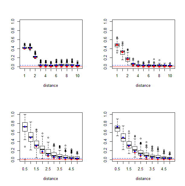
To simulate the Brown-Resnick process in ℝ2\mathbb{R}^{2}, we use RPbrownresnick in the RandomFields package 22 2 http://cran.r-project.org/web/packages/RandomFields/RandomFields.pdf in R. Here, we consider δ⁡(h)=0.5​‖h‖2.\delta(h)=0.5||h||^{2}. In each simulation, first we generate 1600 random locations in {1,…,40}2,\{1,...,40\}^{2}, where the process is simulated with the scale of (1/log⁡(1600))1/a\left({1}/{\log(1600)}\right)^{1/a} and ρ(⋅)=(1+c||⋅||a)−1\displaystyle\rho(\cdot)=(1+c\;||\cdot||^{a})^{-1} with c=1c=1 and a=2a=2. For the ESE computation, we use A=B=(1,∞)A=B=(1,\infty), am=a_{m}= .97 upper quantile. We set w​(⋅)=I[−12,12]​(⋅)w(\cdot)=I_{[-\frac{1}{2},\frac{1}{2}]}(\cdot), and distances h=(0.5,1,…,4.5,5)h=(0.5,1,...,4.5,5). In Figure 2 (right), the extremogram and ESE from one realization are displayed. The extremogram ρA​B​(h){\rho}_{AB}(h) corresponds to connected solid circles and ρ^A​B,m​(h)\hat{\rho}_{AB,m}(h) for different bandwidths λn\lambda_{n} are displayed in different point types. As will be seen in Section 3.3, smaller variances and larger biases are observed for a larger bandwidth. The two horizontal lines are the random permutation bands.

3.3 Simulation study

We use a simulation experiment to examine performances of the ESE. Samples are generated from models with Fréchet marginals for both lattice and non-lattice cases. For lattice cases, we consider MMA(1) and the Brown-Resnick process with δ⁡(h)=0.5​‖h‖2\delta(h)=0.5||h||^{2}. In each simulation, ρ^A​B,m​(h)\hat{\rho}_{AB,m}(h) with A=B=(1,∞)A=B=(1,\infty) and am=a_{m}= .97 upper quantile is calculated for observed distances less than 10. This is repeated 1000 times.
Refer to caption
Figure 3: The distribution of the ESE for MMA(1) on lattice (upper left, 1000 simulations); the Brown-Resnick process on lattice (upper right, 1000 simulations); on ℝ2\mathbb{R}^{2} with λn=1/log⁡n\displaystyle\lambda_{n}={1}/{\log{n}} (bottom left, 100 simulations); and λn=5/log⁡n\displaystyle\lambda_{n}={5}/{\log{n}} (bottom right, 100 simulations). The solid squares are the extremogram. For MMA(1), we see the ESE is centered around PA extremogram (solid circles). For the Brown-Resnick process on ℝ2\mathbb{R}^{2}, we see the impact of bandwidths on the ESE.

Figure 3 (upper left) shows the distributions of ρ^A​B,m​(h)\hat{\rho}_{AB,m}(h) (box plots), ρA​B​(h){\rho}_{AB}(h) (solid squares) and ρA​B,m​(h){\rho}_{AB,m}(h) (solid circles) for MMA(1). In the figure, we see the distributions are centered at ρA​B,m​(h){\rho}_{AB,m}(h), not ρA​B​(h){\rho}_{AB}(h). Notice that ρA​B,m​(h){\rho}_{AB,m}(h) for MMA(1) is computed by

P⁡(Xh>am|X0>am)\displaystyle P(X_{h}>a_{m}|X_{\textbf{0}}>a_{m}) =\displaystyle= 1−2​P​(X0≤am)+P⁡(Xh≤am,X0≤am)P⁡(X0>am)\displaystyle\frac{1-2P(X_{\textbf{0}}\leq a_{m})+P(X_{h}\leq a_{m},X_{\textbf{0}}\leq a_{m})}{P(X_{\textbf{0}}>a_{m})}
=\displaystyle= 2m−1+(1−1m)8/51/m for ​‖h‖=1,2,2m−1+(1−1m)9/51/m for ​‖h‖=2,1m for ​‖h‖>2.\displaystyle\begin{array}[]{ll}\frac{\frac{2}{m}-1+(1-\frac{1}{m})^{8/5}}{1/m}&\text{ for }||h||=1,\sqrt{2},\\ \frac{\frac{2}{m}-1+(1-\frac{1}{m})^{9/5}}{1/m}&\text{ for }||h||=2,\\ \frac{1}{m}&\text{ for }||h||>2.\end{array}

using P⁡(X>am)=1mP(X>a_{m})=\frac{1}{m} and P(X≤x)=e−5/xP(X\leq x)=e^{-5/x} for x>0,x>0, and m=0.03−1.m=0.03^{-1}.

The upper right panel of the figure presents the distributions of the ESE with ρA​B​(h){\rho}_{AB}(h) (solid squares) and ρA​B,m​(h){\rho}_{AB,m}(h) (solid circles) for the Brown-Resnick process on the lattice. The derivation of ρ^A​B,m​(h)\hat{\rho}_{AB,m}(h) is from (3.11). Again, the ESE is centered around PA extremogram.

The bottom panels of Figure 3 are based on the simulation results from the Brown-Resnick process in the non-lattice case. For each simulation, 1600 points are generated from a Poisson process in {1,…,40}2\{1,...,40\}^{2}, from which ρ^A​B,m​(h)\hat{\rho}_{AB,m}(h) for h=(0.5,1,…,4.5,5)h=(0.5,1,...,4.5,5) is computed using the bandwidths λn=1/log⁡n\lambda_{n}={1}/{\log{n}} and 5/log⁡n5/\log{n}. This is repeated 100 times. Notice that the ESE using λn=1/log⁡n\lambda_{n}={1}/{\log{n}} has generally smaller bias but larger variance compared to the ESE using λn=5/log⁡n\lambda_{n}={5}/{\log{n}} for h≤2h\leq 2. For longer lags, the differences is not apparent. This indicates that the ESE with wider bandwidths tends to have smaller variance but larger biases.

Refer to caption
Figure 4: The region of Florida rainfall data.
Figure 5: The locations of extremes (left) and the ESE (right) using the 6 year maxima of Florida rainfall data. For example, the ESE with 0.80 upper quantile (solid line, right) is based on the locations of corresponding extremes (solid circles, left). The ESE using the 0.70 upper quantile indicates that no spatial extremal dependence for lags larger than 3.

4 Application

In this section, we apply the ESE to analyze geographical dependence of heavy rainfall in a region in Florida. The source is Southwest Florida Water Management District. The raw data is total rainfall in 15 minute intervals from 1999 to 2004, measured on a 120 ×\times 120 (km)2 region containing 3600 grid locations. The region of the measurements is shown in Figure 4. For each fixed time, we first calculate the spatial maximum over a non-overlapping block of size 10 ×\times 10 (km)2, which provides a 12 ×\times 12 grid of spatial maxima. Then, we calculate the annual maxima from 1999 to 2004 and the 6 year maxima from the corresponding time series for each spatial maximum. The 7 spatial data sets on a 12 ×\times 12 grid under consideration consist of annual maxima and 6 year maxima of spatial maxima. Since the data are constructed as a maxima over a spatial grid of 25 locations and a temporal resolution of 15 minutes intervals, it is not unreasonable to view these 7 spatial data sets as realizations from a max-stable process.

We first look at the spatial extremal dependence for 6 year maxima rainfall. In Figure 5, the locations of extremes (left) and the ESE (right) are displayed, where the ESE is computed using A=B=(1,∞)A=B=(1,\infty) and am=a_{m}= .70 (dotted line), .75 (dashed line) and .80 (solid line) upper quantiles. Since the number of spatial locations is small (144), we chose modest thresholds in order to ensure enough exceedances for estimation of the ESE. Such thresholds should provide good estimates of the pre-asymptotic extremogram for a max-stable process. The locations of extremes are marked corresponding to choices of ama_{m} by .70 (empty circles), .75 (empty squares) and .80 (solid circles) upper quantiles. For the ESE plot, the horizontal lines are permutation based confidence bands. For example, if extreme events are defined by any rainfall heavier than the .70.70 upper quantile of the maxima rainfall observed for the entire periods, there is a significant extremal dependence between two clusters at distance 2. On the other hand, using the 0.800.80 upper quantile, the extremal dependence at the same distance is no longer significant. In the case of 6 year maxima rainfall, the ESE from the 0.70 upper quantile indicates that no spatial extremal dependence for spatial lags larger than 3. A small spike of the ESE at spatial lags around 4 may be the result of two extremal clusters that are 4 units apart, as seen in the left panel of Figure 5.

By looking at the ESE of annual maxima rainfall from 1999 to 2004, we see year-over-year changes in spatial extremal dependence. Figure 6 presents the locations of extremes and the ESE from 1999 to 2004 (left to right, top to bottom). For example, the ESE suggests that the spatial extremal dependence for lags less than 3 in 2000 is stronger than at any other year between 1999 and 2004. Using the .80 upper quantile, there is significant extremal dependence for spatial lag 8\sqrt{8} in 2000, but not for any other years. In 2002, the spatial extremal dependence is not significant at lag 8\sqrt{8} using the .80 upper quantile. Similarly, the year-to-year comparisons of the ESE with 0.70 and 0.75 upper quantiles confirm that the spatial extremal dependence for spatial lags up to 3 is stronger in 2000 than in any other years.

Figure 6: The ESE of the annual maxima of Florida rainfall from 1999 to 2004 (left to right, top to bottom). The ESE indicates that the spatial extremal dependency for spatial lags less than 3 is the strongest in 2000.

5 Appendix: Proofs

The following proposition presented by Li et al. (2008) is used in the proof. The proposition is analogous to Theorem 17.2.1 in Ibragimov and Linnik (1971).

Proposition 5.1 (Lemma A.1. in Li et al. (2008)).

Let UU and VV be two closed and connected sets in ℝd\mathbb{R}^{d} such that #​U=#​V≤b\#U=\#V\leq b and d⁡(U,V)≥rd(U,V)\geq r for some constants bb and rr. For a stationary process XsX_{s}, consider ξ\xi and η\eta measurable random variables with respect to σ(Xs:s∈U)\sigma(X_{s}:s\in U) and σ(Xs:s∈V)\sigma(X_{s}:s\in V) with |ξ|≤C1,|η|≤C2|\xi|\leq C_{1},|\eta|\leq C_{2}. Then |cov​(ξ,η)|≤4​C1​C2​αb,b​(r)|\text{cov}(\xi,\eta)|\leq 4C_{1}C_{2}\alpha_{b,b}(r).

5.1 Appendix A: Proof of Theorem 2.1

Theorem 2.1 is derived from Theorem 5.2. For notation, we suppress the dependence of mm on nn and write mm for mnm_{n}. Define a vector valued random field by

Yt=XDt,Y_{{t}}=X_{D_{t}}, where Dt=t+Bγ={s∈ℤd:d⁡(t,s)≤γ}D_{t}=t+B_{\gamma}=\{{s}\in\mathbb{Z}^{d}:d({t},{s})\leq\gamma\}.

In Theorem 5.2, we will establish a joint central limit theorem for

P^m(C)=mnnd∑t∈ΛnI{Yt/am∈C}=mnnd∑t∈ΛnpI{Yt/am∈C}+mnnd∑t∈Λn∖ΛnpI{Yt/am∈C},\hat{P}_{m}(C)=\frac{m_{n}}{n^{d}}\sum_{{{t}}\in\Lambda_{n}}I_{\{Y_{{t}}/a_{m}\in C\}}=\frac{m_{n}}{n^{d}}\sum_{{{t}}\in\Lambda_{n}^{p}}I_{\{Y_{{t}}/a_{m}\in C\}}+\frac{m_{n}}{n^{d}}\sum_{{t}\in\Lambda_{n}\setminus\Lambda_{n}^{p}}I_{\{Y_{{t}}/a_{m}\in C\}}, (5.1)

where Λnp={t∈Λn:d⁡(t,∂Λn)≥p}\Lambda_{n}^{p}=\{t\in\Lambda_{n}:d(t,\partial\Lambda_{n})\geq p\} and ∂⁣⋅\partial\cdot denotes the boundary. In fact, showing a CLT for the first term in (5.1) is sufficient as the second term is negligible as n→∞n\rightarrow\infty. Recall that

pm​(A)=m​P​(X0∈am​A)\displaystyle{p}_{m}(A)=mP(X_{\textbf{0}}\in a_{m}A) and τA​B,m​(h)=m​P​(X0∈am​A,Xh∈am​B)\displaystyle{\tau}_{AB,m}(h)=mP(X_{\textbf{0}}\in a_{m}A,X_{h}\in a_{m}B),

where AA and BB are sets bounded away from the origin. Write μ⁡(A)=limn→∞pm​(A)\displaystyle\mu(A)=\lim_{n\rightarrow\infty}{p}_{m}(A),

τA​B​(h)=limn→∞τA​B,m​(h),\displaystyle\tau_{AB}(h)=\lim_{n\rightarrow\infty}{\tau}_{AB,m}(h),
μA​(D0)=limx→∞P⁡(Yt‖Yt‖∈A|‖Yt‖>x),\displaystyle{\mu_{A}(D_{\textbf{0}})=\lim_{x\rightarrow\infty}P\left(\frac{Y_{t}}{\|Y_{t}\|}\in A\Big|\|Y_{t}\|>x\right),}
τA×B​(D0×Dl)=limx→∞P⁡((Y0,Yl)‖vector​{Y0,Yl}‖∈A×B|‖vector​{Y0,Yl}‖>x).\displaystyle{\tau_{A\times B}(D_{\textbf{0}}\times D_{l})=\lim_{x\rightarrow\infty}P\left(\frac{(Y_{{\textbf{0}}},Y_{l})}{\|\text{vector}\{Y_{\textbf{0}},Y_{l}\}\|}\in A\times B\Big|\|\text{vector}\{Y_{\textbf{0}},Y_{l}\}\|>x\right).}
Theorem 5.2.

Assume the conditions of Theorem 2.1. Let C be a set bounded away from zero and a continuity set with respect to μ\mu and τ\tau. Then

Sn=(mnnd)1/2​∑s∈Λn[I⁡(Ysam∈C)−P⁡(Ysam∈C)]→𝑑N⁡(0,σY2​(C))\displaystyle S_{n}=\left(\frac{m_{n}}{n^{d}}\right)^{1/2}\sum_{{s}\in\Lambda_{n}}\left[I\left(\frac{Y_{s}}{a_{m}}\in C\right)-P\left(\frac{Y_{s}}{a_{m}}\in C\right)\right]\xrightarrow{d}{\color[rgb]{0,0,0}N}(0,\sigma_{Y}^{2}(C))

where σY2​(C)=μC​(D0)+∑l≠0∈ℤdτC×C​(D0×Dl).\sigma_{Y}^{2}(C)=\mu_{C}(D_{\textbf{0}})+\sum_{l\neq\textbf{0}\in\mathbb{Z}^{d}}\tau_{C\times C}(D_{\textbf{0}}\times D_{l}).

Proof.

We use ideas from Bolthausen (1982) and Davis and Mikosch (2009) to show the CLT for quantity in (5.1)

P^m​(C)=mn​∑s∈ΛnIs/|Λn|\hat{P}_{m}(C)={m_{n}}\sum_{{s}\in\Lambda_{n}}I_{s}/{|\Lambda_{n}|} where Is=I{Xs/am∈C}I_{s}=I_{\left\{X_{{s}}/a_{m}\in C\right\}}.

The proof for the CLT of XsX_{s} replaced by a vector valued random field YsY_{s} in indicator is analogous.

Define H⁡[a,b]={d⁡(s,t):a≤d⁡(s,t)≤b}H[a,b]=\{d(s,t):a\leq d(s,t)\leq b\} and ‖l‖=d⁡(0,l)||l||=d(\textbf{0},l) for convenience. Assume mn2+2​d=o⁡(nd)m_{n}^{2+2d}=o({n^{d}}), rnd=o⁡(mn),r_{n}^{d}=o({m_{n}}), and

limk→∞lim supn→∞mn∑l∈ℤd,||l||∈H(k,rn]P(|Xl|>εam,|X0|>εam)=0for∀ϵ>0,\displaystyle\lim_{k\rightarrow\infty}\displaystyle\limsup_{n\rightarrow\infty}m_{n}\sum_{l\in\mathbb{Z}^{d},||l||\in H(k,r_{n}]}P(|X_{{l}}|>\varepsilon a_{m},|X_{{\textbf{0}}}|>\varepsilon a_{m})=0\quad\text{for}\quad\forall\epsilon>0, (5.2)
limn→∞mn​∑l∈ℤd,‖l‖∈H⁡(rn,∞)α1,1​(‖l‖)=0,\displaystyle\lim_{n\rightarrow\infty}m_{n}\sum_{l\in\mathbb{Z}^{d},||l||\in H(r_{n},\infty)}\alpha_{1,1}(||l||)=0, (5.3)
∑l∈ℤdαj1,j2​(‖l‖)<∞for2≤j1+j2≤4,\displaystyle{\sum_{l\in\mathbb{Z}^{d}}\alpha_{j_{1},j_{2}}(||l||)<\infty\quad\text{for}\quad 2\leq j_{1}+j_{2}\leq 4,} (5.4)
limn→∞nd/2​mn1/2​α1,nd​(mn)=0,\displaystyle\lim_{n\rightarrow\infty}n^{d/2}m_{n}^{1/2}\alpha_{1,n^{d}}(m_{n})=0, (5.5)

which are univariate case analog of conditions (2.1) - (2.4).

By the same arguments in Davis and Mikosch (2009),

E​P^m​(C)→μ⁡(C)\displaystyle E\hat{P}_{m}(C)\rightarrow\mu(C) (5.6)
var​(P^m​(C))∼mnnd​[μ⁡(C)+∑l≠0∈ℤdτC​C​(l)]=mnnd​σX2​(C),\displaystyle\text{var}\left(\hat{P}_{m}(C)\right)\sim\displaystyle\frac{m_{n}}{n^{d}}\left[\mu(C)+{\sum_{l\neq\textbf{0}\in\mathbb{Z}^{d}}}\tau_{CC}(l)\right]=\frac{m_{n}}{n^{d}}\;\sigma_{X}^{2}(C), (5.7)

where (5.6) is implied by the regularly varying assumption. To see (5.7), observe that

ndmn​var​(P^m​(C))=mnnd​∑s∈Λnvar​(Is)+mnnd​∑s,t∈Λn,s≠tcov​(Is,It)=A1+A2.\displaystyle\frac{n^{d}}{m_{n}}\text{var}\left(\hat{P}_{m}(C)\right)=\frac{m_{n}}{n^{d}}\sum_{s\in\Lambda_{n}}\text{var}(I_{s})+\frac{m_{n}}{n^{d}}\sum_{s,t\in\Lambda_{n},s\neq t}\text{cov}(I_{s},I_{t})=A_{1}+A_{2}. (5.8)

By the regularly varying assumption, A1=pm​(C)+(pm​(C))2/mn→μ⁡(C).A_{1}=p_{m}(C)+(p_{m}(C))^{2}/m_{n}\rightarrow\mu(C). Turning to A2A_{2}, for k≥1k\geq 1 fixed,

A2\displaystyle A_{2} ∼\displaystyle\sim mnnd​∑l=(l1,…​ld)≠0,‖l‖≤max⁡ΛnΠi=1d​(n−|li|)​cov​(I0,Il)\displaystyle\frac{m_{n}}{n^{d}}\sum_{l=(l_{1},...l_{d})\neq\textbf{0},||l||\leq\max\Lambda_{n}}\Pi_{i=1}^{d}(n-|l_{i}|)\text{cov}(I_{\textbf{0}},I_{l})
=\displaystyle= mnnd[∑l∈ℤd,||l||∈H(0,k]⋅+∑l∈ℤd,||l||∈H(k,rn]⋅+∑l∈ℤd,||l||∈H(rn,maxΛn]⋅]=A21+A22+A23\displaystyle\frac{m_{n}}{n^{d}}\left[\sum_{l\in\mathbb{Z}^{d},||l||\in H(0,k]}\cdot+\sum_{l\in\mathbb{Z}^{d},||l||\in H(k,r_{n}]}\cdot+\sum_{l\in\mathbb{Z}^{d},||l||\in H(r_{n},\max\Lambda_{n}]}\cdot\right]=A_{21}+A_{22}+A_{23}

where maxΛn={max(d(s,t)):s,t∈Λn}\max\Lambda_{n}=\{\max(d(s,t)):s,t\in\Lambda_{n}\} and Πi=1d​(n−|li|)\Pi_{i=1}^{d}(n-|l_{i}|) counts a number of cubes with lag ll in Λn\Lambda_{n}.

From the regularly varying assumption, limk→∞lim supn→∞A21=∑l≠0∈ℤdτC​C​(l)\displaystyle\lim_{k\rightarrow\infty}\limsup_{n\rightarrow\infty}A_{21}=\sum_{l\neq{\textbf{0}}\in\mathbb{Z}^{d}}\tau_{CC}(l) since

lim supn→∞A21=∑l∈ℤd,||l||∈H(0,k]lim supn→∞(τC​C,m(C)−pm(C)pm​(C)mn)=∑l∈ℤd,||l||∈H(0,k]τC​C(l).\displaystyle\limsup_{n\rightarrow\infty}A_{21}=\sum_{l\in\mathbb{Z}^{d},||l||\in H(0,k]}\limsup_{n\rightarrow\infty}\left(\tau_{CC,m}(C)-p_{m}(C)\frac{p_{m}(C)}{m_{n}}\right)=\sum_{l\in\mathbb{Z}^{d},||l||\in H(0,k]}\tau_{CC}(l).

Thus, it is sufficient to show

limk→∞lim supn→∞(|A22|+|A23|)=0\displaystyle\lim_{k\rightarrow\infty}\limsup_{n\rightarrow\infty}(|A_{22}|+|A_{23}|)=0

to achieve (5.7). Recall that CC is bounded away from the origin. Notice that

A22\displaystyle A_{22} ≤\displaystyle\leq constmn∑l∈ℤd,||l||∈H(k,rn][P(|Xl|>εam,|X0|>εam)+(pm​(C)mn)2],\displaystyle const\;m_{n}\sum_{l\in\mathbb{Z}^{d},||l||\in H(k,r_{n}]}\left[P(|X_{l}|>\varepsilon a_{m},|X_{\textbf{0}}|>\varepsilon a_{m})+\left(\frac{p_{m}(C)}{m_{n}}\right)^{2}\right],
A23\displaystyle A_{23} ≤\displaystyle\leq c​o​n​s​t​mn​∑l∈ℤd,‖l‖∈H⁡(rn,∞)α1,1​(‖l‖),\displaystyle const\;m_{n}\sum_{l\in\mathbb{Z}^{d},||l||\in H(r_{n},\infty)}\alpha_{1,1}(||l||),

so (5.7) holds assuming (5.2), (5.3) and rnd/mn→0.r_{n}^{d}/m_{n}\rightarrow 0.

Now, we prove

ndmn​(P^m​(C)−pm​(C))=mnnd​∑s∈ΛnI¯s→𝑑N⁡(0,σX2​(C))\displaystyle{\sqrt{\frac{n^{d}}{m_{n}}}(\hat{P}_{m}(C)-p_{m}(C))=\sqrt{\frac{m_{n}}{n^{d}}}\sum_{{s}\in\Lambda_{n}}\bar{I}_{s}\xrightarrow{d}N(0,\sigma_{X}^{2}(C))} (5.9)

where I¯t=I⁡(Xtam∈C)−P⁡(Xam∈C)\bar{I}_{t}=I\left(\frac{X_{t}}{a_{m}}\in C\right)-P\left(\frac{X}{a_{m}}\in C\right). First, infer from (5.8) that

mnnd​∑s,t∈Λn|cov​(I¯s,I¯t)|<∞.\displaystyle{\frac{m_{n}}{n^{d}}}\sum_{s,t\in\Lambda_{n}}|\text{cov}(\bar{I}_{s},\bar{I}_{t})|<\infty. (5.10)

As the next step, define

Sα,n=∑β∈Λn,d⁡(α,β)≤mnmnndI¯β,vn=∑α∈ΛnE(mnndI¯αSα,n),S¯n=vn−1/2Sn,andS¯α,n=vn−1/2Sα,n.\displaystyle S_{\alpha,n}=\sum_{\beta\in\Lambda_{n},d(\alpha,\beta)\leq m_{n}}\sqrt{\frac{m_{n}}{n^{d}}}\bar{I}_{\beta},\;v_{n}=\sum_{\alpha\in\Lambda_{n}}E(\sqrt{\frac{m_{n}}{n^{d}}}\bar{I}_{\alpha}S_{\alpha,n}),\;\bar{S}_{n}=v_{n}^{-1/2}S_{n},\;\text{and}\;\bar{S}_{\alpha,n}=v_{n}^{-1/2}S_{\alpha,n}.

From the definition, vn∼var​(Sn)→σ2​(C)\displaystyle v_{n}\sim{\text{var}(S_{n})}\rightarrow\sigma^{2}(C).

Now, use Stein’s lemma to show (5.9) as in Bolthausen (1982) by checking limn→∞E⁡((i​λ−S¯n)​ei​λ​S¯n)=0\lim_{n\rightarrow\infty}E((i\lambda-\bar{S}_{n})e^{i\lambda\bar{S}_{n}})=0 for all λ∈R\lambda\in R. Write

(i​λ−S¯n)​ei​λ​S¯n\displaystyle(i\lambda-\bar{S}_{n})e^{i\lambda\bar{S}_{n}} =\displaystyle= iλei​λ​S¯n(1−vn−1∑α∈ΛnmnndI¯αSα,n)−vn−1/2ei​λ​S¯n∑α∈ΛnmnndI¯α[1−e−i​λ​S¯α,n−iλS¯α,n]\displaystyle i\lambda e^{i\lambda\bar{S}_{n}}(1-v_{n}^{-1}\sum_{\alpha\in\Lambda_{n}}\sqrt{\frac{m_{n}}{n^{d}}}\bar{I}_{\alpha}{S}_{\alpha,n})-v_{n}^{-1/2}e^{i\lambda\bar{S}_{n}}\sum_{\alpha\in\Lambda_{n}}\sqrt{\frac{m_{n}}{n^{d}}}\bar{I}_{\alpha}[1-e^{-i\lambda\bar{S}_{\alpha,n}}-i\lambda\bar{S}_{\alpha,n}]
−vn−1/2∑α∈ΛnmnndI¯αe−i​λ​(S¯n−S¯α,n)\displaystyle\qquad\qquad\qquad\qquad\qquad\qquad-v_{n}^{-1/2}\sum_{\alpha\in\Lambda_{n}}\sqrt{\frac{m_{n}}{n^{d}}}\bar{I}_{\alpha}e^{-i\lambda(\bar{S}_{n}-\bar{S}_{\alpha,n})}
=\displaystyle= B1+B2+B3.\displaystyle B_{1}+B_{2}+B_{3}.

We will show E​|B1|2→0E|B_{1}|^{2}\rightarrow 0. From Proposition 5.1, when d⁡(α,α′)≥3​mnd(\alpha,\alpha^{\prime})\geq 3m_{n},

|cov​(I¯α​I¯β,I¯α′​I¯β′)|\displaystyle|\text{cov}(\bar{I}_{\alpha}\bar{I}_{\beta},\bar{I}_{\alpha^{\prime}}\bar{I}_{\beta^{\prime}})| ≤\displaystyle\leq 4​α2,2​(d⁡(α,α′)−2​mn).\displaystyle 4\;\alpha_{2,2}(d(\alpha,\alpha^{\prime})-2m_{n}).

When d⁡(α,α′)<3​mn,d(\alpha,\alpha^{\prime})<3m_{n}, let j=min⁡{d⁡(α,α′),d⁡(α,β′),d⁡(β,α′),d⁡(β,β′)}j=\min\{d(\alpha,\alpha^{\prime}),d(\alpha,\beta^{\prime}),d(\beta,\alpha^{\prime}),d(\beta,\beta^{\prime})\}. Then

|cov​(I¯α​I¯β,I¯α′​I¯β′)|\displaystyle|\text{cov}(\bar{I}_{\alpha}\bar{I}_{\beta},\bar{I}_{\alpha^{\prime}}\bar{I}_{\beta^{\prime}})| ≤\displaystyle\leq 4​αp,q​(j)\displaystyle 4\;\alpha_{p,q}(j)

for 2≤p+q≤4.2\leq p+q\leq 4. Given mn2+2​d=o⁡(nd)m_{n}^{2+2d}=o(n^{d}), we have E​|B1|2→0E|B_{1}|^{2}\rightarrow 0 since

E​|B1|2\displaystyle E|B_{1}|^{2} (5.11)
=\displaystyle= λ2​vn−2​∑α,α′,β,β′,d⁡(α,β)≤mn,d⁡(α′,β′)≤mnmn2n2​d​cov​(I¯α​I¯β,I¯α′​I¯β′)\displaystyle\lambda^{2}v_{n}^{-2}\sum_{\alpha,\alpha^{\prime},\beta,\beta^{\prime},d(\alpha,\beta)\leq m_{n},d(\alpha^{\prime},\beta^{\prime})\leq m_{n}}\frac{m_{n}^{2}}{n^{2d}}\;\text{cov}(\bar{I}_{\alpha}\bar{I}_{\beta},\bar{I}_{\alpha^{\prime}}\bar{I}_{\beta^{\prime}})
≤\displaystyle\leq λ2vn2mn2n2​d[∑α∈Λn∑α′∈Λn∩{d(α,α′)>3mn}∑β,β′|cov(I¯αI¯β,I¯α′I¯β′)|+∑α∈Λn∑α′∈Λn∩{d(α,α′)≤3mn}∑β,β′|cov(I¯αI¯β,I¯α′I¯β′)|]\displaystyle\frac{\lambda^{2}}{v_{n}^{2}}\frac{m_{n}^{2}}{n^{2d}}\;\left[\sum_{\alpha\in\Lambda_{n}}\sum_{\alpha^{\prime}\in\Lambda_{n}\cap\{d(\alpha,\alpha^{\prime})>3m_{n}\}}\sum_{\beta,\beta^{\prime}}\left|\text{cov}(\bar{I}_{\alpha}\bar{I}_{\beta},\bar{I}_{\alpha^{\prime}}\bar{I}_{\beta^{\prime}})\right|+\sum_{\alpha\in\Lambda_{n}}\sum_{\alpha^{\prime}\in\Lambda_{n}\cap\{d(\alpha,\alpha^{\prime})\leq 3m_{n}\}}\sum_{\beta,\beta^{\prime}}\left|\text{cov}(\bar{I}_{\alpha}\bar{I}_{\beta},\bar{I}_{\alpha^{\prime}}\bar{I}_{\beta^{\prime}})\right|\right]
≤\displaystyle\leq λ2vn2mn2n2​d 4[∑α∈Λn∑α′∈Λn∩{d(α,α′)>3mn}∑β,β′α2,2(d(α,α′)−2mn)+∑α∈Λn∑α′∈Λn∩{d(α,α′)≤3mn}∑β,β′αp,q(j)]\displaystyle\frac{\lambda^{2}}{v_{n}^{2}}\frac{m_{n}^{2}}{n^{2d}}\;4\;\left[\sum_{\alpha\in\Lambda_{n}}\sum_{\alpha^{\prime}\in\Lambda_{n}\cap\{d(\alpha,\alpha^{\prime})>3m_{n}\}}\sum_{\beta,\beta^{\prime}}\alpha_{2,2}(d(\alpha,\alpha^{\prime})-2m_{n})+\sum_{\alpha\in\Lambda_{n}}\sum_{\alpha^{\prime}\in\Lambda_{n}\cap\{d(\alpha,\alpha^{\prime})\leq 3m_{n}\}}\sum_{\beta,\beta^{\prime}}\alpha_{p,q}(j)\right]\;
≤\displaystyle\leq c​o​n​s​t​λ2​mn2vn2​n2​d​nd​mn2​d​[∑l∈ℤd,‖l‖∈H⁡(3​mn,∞)α2,2​(‖l‖−2​mn)+∑l∈ℤd,‖l‖∈H⁡[0,3​mn]αp,q​(‖l‖)]\displaystyle\frac{const\lambda^{2}m_{n}^{2}}{v_{n}^{2}n^{2d}}n^{d}m_{n}^{2d}\;\left[\sum_{l\in\mathbb{Z}^{d},||l||\in H(3m_{n},\infty)}\alpha_{2,2}(||l||-2m_{n})+\;\sum_{l\in\mathbb{Z}^{d},||l||\in H[0,3m_{n}]}\alpha_{p,q}(||l||)\right]\;
=\displaystyle= O⁡(mn2+2​d/nd).\displaystyle O(m_{n}^{2+2d}/n^{d}).

Notice that in (5.11), nd​mn2​dn^{d}m_{n}^{2d} is from summing over α\alpha (giving ndn^{d}), β\beta (giving O⁡(mnd)O(m_{n}^{d})), and β′\beta^{\prime} (giving O⁡(mnd)O(m_{n}^{d})) for the first summation. Similarly, for the second summation, nd​mn2​dn^{d}m_{n}^{2d} is from summing over α,β\alpha,\beta and α′​or​β′\alpha^{\prime}\;\text{or}\;\beta^{\prime} depending on the location of points. The last equation is from (5.4).

Now we show E​|B2|→0E|B_{2}|\rightarrow 0 provided mn2+2​d=o⁡(nd)m_{n}^{2+2d}=o(n^{d}). Recall that |ei​x−1−i​x|≤12​x2|e^{ix}-1-ix|\leq\frac{1}{2}x^{2}. Then

E​|B2|\displaystyle E|B_{2}| ≤\displaystyle\leq cvn−1/2ndmnndES¯α,n2\displaystyle cv_{n}^{-1/2}n^{d}\sqrt{\frac{m_{n}}{n^{d}}}E\bar{S}_{\alpha,n}^{2}
=\displaystyle= cvn−1/2mnndmn∑β,β′,d⁡(0,β)≤mn,d⁡(0,β′)≤mnE(I¯βI¯β′)\displaystyle cv_{n}^{-1/2}\sqrt{\frac{m_{n}}{n^{d}}}m_{n}\sum_{\beta,\beta^{\prime},d(\textbf{0},\beta)\leq m_{n},d(\textbf{0},\beta^{\prime})\leq m_{n}}{E(\bar{I}_{\beta}\bar{I}_{\beta^{\prime}})}
≤\displaystyle\leq c​mnnd​mnd+1​∑l∈ΛnE⁡(I¯0​I¯l)\displaystyle c\sqrt{\frac{m_{n}}{n^{d}}}m_{n}^{d+1}\sum_{l\in\Lambda_{n}}{E(\bar{I}_{{\textbf{0}}}\bar{I}_{l})}
=\displaystyle= O⁡(mn1+2​dnd)\displaystyle O\left(\sqrt{\frac{m_{n}^{1+2d}}{n^{d}}}\right)

where mn​∑l∈ΛnE⁡(I¯0​I¯l)<∞m_{n}\sum_{l\in\Lambda_{n}}{E(\bar{I}_{{\textbf{0}}}\bar{I}_{l})}<\infty is inferred from (5.10).

Lastly, the condition (5.5) implies |E​B3|→0|EB_{3}|\rightarrow 0 since

|E​B3|\displaystyle|EB_{3}| ≤\displaystyle\leq cvn−1/2ndmnndα1,nd(mn)=cnd/2mn1/2α1,nd(mn).\displaystyle cv_{n}^{-1/2}n^{d}\sqrt{\frac{m_{n}}{n^{d}}}\alpha_{1,n^{d}}(m_{n})=cn^{d/2}m_{n}^{1/2}\alpha_{1,n^{d}}(m_{n}).

Thus, Stein’s lemma is satisfied, which completes the proof. ∎

Remark 4.

P^m​(C)\hat{P}_{m}(C) is a consistent estimator of μ⁡(C).\mu(C). If μ⁡(C)=0,\mu(C)=0, var (P^m​(C))=o⁡(mn/nd)(\hat{P}_{m}(C))=o(m_{n}/n^{d}).

Remark 5.

The conditions (2.1) - (2.4) are derived from (5.2) - (5.5) by replacing univariate process (XtX_{{t}}) by vectorized process (YtY_{{t}}). In order to see (2.1) is derived from (5.2), for example, consider Euclidean norm for (YtY_{{t}}) process. Then, the vectorized analog of (5.2) is

limk→∞lim supn→∞mn∑l∈ℤd,||l||∈H(k,rn]P(||Y0||>ϵam,||Yl||>ϵam)=0\displaystyle\lim_{k\rightarrow\infty}\limsup_{n\rightarrow\infty}m_{n}\sum_{l\in\mathbb{Z}^{d},||l||\in H(k,r_{n}]}P(||Y_{{\textbf{0}}}||>\epsilon a_{m},||Y_{{l}}||>\epsilon a_{m})=0,

which holds under (2.1) by triangular inequality, i.e.,

P⁡(‖Y0‖>ϵ​am,‖Yl‖>ϵ​am)\displaystyle\displaystyle P(||Y_{\textbf{0}}||>\epsilon a_{m},||Y_{{l}}||>\epsilon a_{m}) ≤\displaystyle\leq P(∑s∈D0|Xs|>ϵam,∑s′∈Dl|Xs′|>ϵam)≤P(maxs∈D0|Xs|>ϵ​am|D0|,maxs′∈Dl|Xs′|>ϵ​am|Dl|).\displaystyle P(\sum_{{s}\in D_{\textbf{0}}}|X_{{s}}|>\epsilon a_{m},\sum_{{s}^{\prime}\in D_{l}}|X_{s^{\prime}}|>\epsilon a_{m})\leq P\left(\max_{{s}\in D_{\textbf{0}}}|X_{{s}}|>\frac{\epsilon a_{m}}{|D_{\textbf{0}}|},\max_{{s}^{\prime}\in D_{l}}|X_{{s}^{\prime}}|>\frac{\epsilon a_{m}}{|D_{l}|}\right).

The rest of the derivations are straightforward.

Proof of Theorem 2.1.

Apply the Cramér-Wold device to Theorem 5.2 to achieve the multivariate central limit theorem, then use δ\delta-method to obtain the central limit theorem for the ESE. To specify the limiting variance Σ\Sigma, redefine

μ⁡(A)=limx→∞P⁡(Xt‖Yt‖∈A|‖Yt‖>x).\displaystyle\mu(A)=\lim_{x\rightarrow\infty}P\left(\frac{X_{t}}{\|Y_{t}\|}\in A\Big|\|Y_{t}\|>x\right).

Then, Σ=μ​(A)−4​F​Π​Ft\Sigma=\mu(A)^{-4}{F}\Pi{F}^{t} where

Πi,i\displaystyle\Pi_{i,i} =\displaystyle= μSi​(D0)+∑l≠0∈ℤdτSi×Si​(D0×Dl)\displaystyle\mu_{S_{i}}(D_{\textbf{0}})+\sum_{l\neq{\textbf{0}}\in\mathbb{Z}^{d}}\tau_{S_{i}\times S_{i}}(D_{\textbf{0}}\times D_{l})
Πi,j\displaystyle\Pi_{i,j} =\displaystyle= μSi∩Sj​(D0)+∑l≠0∈ℤdτSi×Sj​(D0×Dl)\displaystyle\mu_{S_{i}\cap S_{j}}(D_{\textbf{0}})+\sum_{l\neq{\textbf{0}}\in\mathbb{Z}^{d}}\tau_{S_{i}\times S_{j}}(D_{\textbf{0}}\times D_{l})
F\displaystyle F =\displaystyle= (μ⁡(S(#​H)+1)00...0−μS1​(D0)0μ⁡(S(#​H)+1)0...0−μS2​(D0)................000...μ⁡(S(#​H)+1)−μS(#​H)​(D0))\displaystyle\begin{pmatrix}\mu(S_{(\#H)+1})&0&0&...&0&-\mu_{S_{1}}(D_{\textbf{0}})\\ 0&\mu(S_{(\#H)+1})&0&...&0&-\mu_{S_{2}}(D_{\textbf{0}})\\ .&.&.&...&.&.\\ .&.&.&...&.&.\\ 0&0&0&...&\mu(S_{(\#H)+1})&-\mu_{S_{(\#H)}}(D_{\textbf{0}})\end{pmatrix}

where the sets SiS_{i} are chosen such that {Yt∈Si}={Xt∈A,Xs∈B:d(t,s)=hi}\{Y_{t}\in S_{i}\}=\{X_{t}\in A,X_{s}\in B:d(t,s)=h_{i}\} for hi∈Hh_{i}\in H and i=1,…,(#​H)i=1,...,(\#H) and {Yt∈S(#​H)+1}={Xt∈A}\{Y_{t}\in S_{(\#H)+1}\}=\{X_{t}\in A\}. For more details, see Davis and Mikosch (2009). ∎

5.2 Appendix B: Proof of Theorem 2.3

Theorem 2.3 is derived from Proposition 5.4 - 5.6. Before proceeding to Proposition 5.4, we present the following result regarding LUNC.

Proposition 5.3.

Consider a strictly stationary regularly varying random field {Xs,s∈ℝd}\{X_{s},s\in\mathbb{R}^{d}\} with index α>0\alpha>0 satisfying LUNC. For a positive integer kk and λn→0\lambda_{n}\rightarrow 0,

n​P​(X0an∈A0,Xs1+λnan∈A1,⋯,Xsk+λnan∈Ak)→τA0,A1,⋯,Ak​(s1,⋯,sk)\displaystyle nP\left(\frac{X_{\textbf{0}}}{a_{n}}\in A_{0},\frac{X_{s_{1}+\lambda_{n}}}{a_{n}}\in A_{1},\cdots,\frac{X_{s_{k}+\lambda_{n}}}{a_{n}}\in A_{k}\right)\rightarrow\tau_{A_{0},A_{1},\cdots,A_{k}}(s_{1},\cdots,s_{k})

provided A0×A1×⋯×AkA_{0}\times A_{1}\times\cdots\times A_{k} is a continuity set of the limit measure

τA0,A1,⋯,Ak(s1,⋯,sk)=limn→∞nP(X0/an∈A0,Xs1/an∈A1,⋯,Xsk/an∈Ak).\displaystyle\tau_{A_{0},A_{1},\cdots,A_{k}}(s_{1},\cdots,s_{k})=\lim_{n\rightarrow\infty}nP\left({X_{\textbf{0}}}/{a_{n}}\in A_{0},{X_{s_{1}}}/{a_{n}}\in A_{1},\cdots,{X_{s_{k}}}/{a_{n}}\in A_{k}\right).
Proof.

Let ff be a continuous function with compact support on ℝ¯k+1∖{0}.\bar{\mathbb{R}}^{k+1}\setminus\{{\textbf{0}}\}. Since ff has compact support, it is uniformly continuous and hence for every ϵ>0\epsilon>0 there exists δ\delta such that |f⁡(x1,x2,⋯,xk+1)−f⁡(y1,y2,⋯,yk+1)|<ϵ|f(x_{1},x_{2},\cdots,x_{k+1})-f(y_{1},y_{2},\cdots,y_{k+1})|<\epsilon whenever |(x1,x2,⋯,xk+1)−(y1,y2,⋯,yk+1)|<δ.|(x_{1},x_{2},\cdots,x_{k+1})-(y_{1},y_{2},\cdots,y_{k+1})|<\delta.

Let X~n=(X0,Xs1+λn,⋯,Xsk+λn)\tilde{X}_{n}=(X_{\textbf{0}},X_{s_{1}+\lambda_{n}},\cdots,X_{s_{k}+\lambda_{n}}) and X~=(X0,Xs1,⋯,Xsk)\tilde{X}=(X_{\textbf{0}},X_{s_{1}},\cdots,X_{s_{k}}). Notice that

n​E​|f⁡(X~nan)−f⁡(X~an)|\displaystyle nE\left|f\left(\frac{\tilde{X}_{n}}{a_{n}}\right)-f\left(\frac{\tilde{X}}{a_{n}}\right)\right| =\displaystyle= nE|⋅|I{|X~n−X~|an>δ}+nE|⋅|I{|X~n−X~|an≤δ}=A1+A2.\displaystyle nE|\cdot|I_{\{\frac{|\tilde{X}_{n}-\tilde{X}|}{a_{n}}>\delta\}}+nE|\cdot|I_{\{\frac{|\tilde{X}_{n}-\tilde{X}|}{a_{n}}\leq\delta\}}=A_{1}+A_{2}.

Let M=max⁡f⁡(Xan).M=\max f\left(\frac{\textbf{X}}{a_{n}}\right). By (2.17), there exists ϵ>0\epsilon>0 such that

lim supnA1\displaystyle\limsup_{n}A_{1} ≤\displaystyle\leq lim supn2​M​n​[P⁡(|Xs1+λn−Xs1|>δ​ank)+⋯+P⁡(|Xsk+λn−Xsk|>δ​ank)]<2​M​ϵ\displaystyle\limsup_{n}2Mn\left[P\left(|X_{s_{1}+\lambda_{n}}-X_{s_{1}}|>\frac{\delta a_{n}}{k}\right)+\cdots+P\left(|X_{s_{k}+\lambda_{n}}-X_{s_{k}}|>\frac{\delta a_{n}}{k}\right)\right]<2M\epsilon

since |Xλn−X0|≤sup|s|<δ′|Xs−X0||X_{\lambda_{n}}-X_{\textbf{0}}|\leq\sup_{|s|<\delta^{\prime}}|X_{s}-X_{\textbf{0}}| as n→∞n\rightarrow\infty for |λn|<δ′|\lambda_{n}|<\delta^{\prime}. For A2A_{2}, since the support of f∈{|X~|>C}⊂{|X0|>Ck+1}∪⋯∪{|Xsk|>Ck+1}f\in\{|\tilde{X}|>C\}\subset\{|X_{\textbf{0}}|>\frac{C}{k+1}\}\cup\cdots\cup\{|X_{s_{k}}|>\frac{C}{k+1}\}

lim supnA2\displaystyle\limsup_{n}A_{2} ≤\displaystyle\leq lim supnϵ​n​[P⁡(|X~n|an>C)+P⁡(|X~|an>C)]\displaystyle\limsup_{n}\epsilon n\left[P\left(\frac{|\tilde{X}_{n}|}{a_{n}}>C\right)+P\left(\frac{|\tilde{X}|}{a_{n}}>C\right)\right]
=\displaystyle= lim supnϵ​n​ 2​(k+1)​P​(|X0|>an​C/(k+1))\displaystyle\limsup_{n}\epsilon\;n\;2(k+1)\;P\left({|X_{\textbf{0}}|}>a_{n}C/(k+1)\right)
=\displaystyle= ϵ​ 2​(k+1)​τB​B​(0),where​B={x:x>C/(k+1)}.\displaystyle\epsilon\;2({k+1})\tau_{BB}(\textbf{0}),\qquad\text{where}\;B=\{x:x>C/(k+1)\}.

Take ϵ\epsilon small by choosing appropriate δ\delta and δ′\delta^{\prime}, then for a positive integer kk and λn→0\lambda_{n}\rightarrow 0,

n​E​f​(X0,Xs1+λn,⋯,Xsk+λnan)→∫f⁡(u1,u2,⋯,uk)​μ​(d​u1,d​u2,⋯,d​uk)\displaystyle nEf\left(\frac{X_{\textbf{0}},X_{s_{1}+\lambda_{n}},\cdots,X_{s_{k}+\lambda_{n}}}{a_{n}}\right)\rightarrow\int f(u_{1},u_{2},\cdots,u_{k})\mu(du_{1},du_{2},\cdots,du_{k})

for any continuous function with compact support ff. Using Portmanteau theorem for vague convergence, we complete the proof. See Theorem 3.2 in Resnick (2006). ∎

We discuss asymptotics of the denominator and the numerator of the ESE in turn.

Proposition 5.4.

Under the setting of Theorem 2.3 and condition (M2),

E⁡(p^m​(A))=pm​(A)→μ⁡(A)\displaystyle E(\hat{p}_{m}(A))=p_{m}(A)\rightarrow\mu(A)\quad and |Sn|mn​var​(p^m​(A))→μ⁡(A)ν+∫ℝ2τA​A​(y)​𝑑y\quad\displaystyle\frac{|S_{n}|}{m_{n}}{\text{var}}(\hat{p}_{m}(A))\rightarrow\frac{\mu(A)}{\nu}+\int_{\mathbb{R}^{2}}\tau_{AA}(y)dy.

Hence, p^m​(A)→𝑝μ​(A)\hat{p}_{m}(A)\xrightarrow{p}\mu(A).

Proof.

By the regularly varying property, E⁡(p^m​(A))=pm​(A)→μ⁡(A)E(\hat{p}_{m}(A))=p_{m}(A)\rightarrow\mu(A).

For var​(p^m​(A))\text{var}(\hat{p}_{m}(A)), recall that N(2)​(d​s1,d​s2)=N⁡(d​s1)​N​(d​s2)​I​(s1≠s2)N^{(2)}(ds_{1},ds_{2})=N(ds_{1})N(ds_{2})I(s_{1}\neq s_{2}) and observe that

E⁡(p^m​(A)2)\displaystyle E(\hat{p}_{m}(A)^{2})
=(mnν​|Sn|)2​E​[∫SnI⁡(Xs1am∈A)​N​(d​s1)+∫Sn∫SnI⁡(Xs1am∈A,Xs2am∈A)​N(2)​(d​s1,d​s2)]\displaystyle\quad=\left(\frac{m_{n}}{\nu|S_{n}|}\right)^{2}E\left[\int_{S_{n}}I\left(\frac{X_{s_{1}}}{a_{m}}\in A\right)N(ds_{1})+\int_{S_{n}}\int_{S_{n}}I\left(\frac{X_{s_{1}}}{a_{m}}\in A,\frac{X_{s_{2}}}{a_{m}}\in A\right)N^{(2)}(ds_{1},ds_{2})\right]
=(mnν​|Sn|)2​[∫Snpm​(A)mn​ν​d​s1+∫Sn∫Sn[P⁡(Xs1am∈A,Xs2am∈A)−pm​(A)2mn2]​ν2​d​s1​d​s2]+E​(p^m​(A))2\displaystyle\quad=\left(\frac{m_{n}}{\nu|S_{n}|}\right)^{2}\left[\int_{S_{n}}\frac{{p}_{m}(A)}{m_{n}}\nu ds_{1}+\int_{S_{n}}\int_{S_{n}}\left[P\left(\frac{X_{s_{1}}}{a_{m}}\in A,\frac{X_{s_{2}}}{a_{m}}\in A\right)-\frac{{p}_{m}(A)^{2}}{m_{n}^{2}}\right]\nu^{2}ds_{1}ds_{2}\right]+E(\hat{p}_{m}(A))^{2}
=(mn|Sn|)​[E​(p^m​(A))ν+∫Sn−Snmn​[τA​A,m​(y)mn−pm​(A)2mn2]​|Sn∩(Sn−y)||Sn|​𝑑y]+E​(p^m​(A))2\displaystyle\quad=\left(\frac{m_{n}}{|S_{n}|}\right)\left[\frac{E(\hat{p}_{m}(A))}{\nu}+\int_{S_{n}-S_{n}}m_{n}\left[\frac{{\tau}_{AA,m}(y)}{m_{n}}-\frac{{p}_{m}(A)^{2}}{m_{n}^{2}}\right]\frac{|S_{n}\cap(S_{n}-y)|}{|S_{n}|}dy\right]+E(\hat{p}_{m}(A))^{2}

where the change of variables s2−s1=ys_{2}-s_{1}=y is used in the last line. Using the above, we show

|Sn|mn​var​(p^m​(A))\displaystyle\frac{|S_{n}|}{m_{n}}\text{var}(\hat{p}_{m}(A)) =\displaystyle= E​(p^m​(A))ν+∫Sn−Snmn​[τA​A,m​(y)mn−pm​(A)2mn2]​|Sn∩(Sn−y)||Sn|​𝑑y\displaystyle\frac{E(\hat{p}_{m}(A))}{\nu}+\int_{S_{n}-S_{n}}m_{n}\left[\frac{{\tau}_{AA,m}(y)}{m_{n}}-\frac{{p}_{m}(A)^{2}}{m_{n}^{2}}\right]\frac{|S_{n}\cap(S_{n}-y)|}{|S_{n}|}dy (5.12)
→\displaystyle\rightarrow μ⁡(A)ν+∫ℝ2τA​A​(y)​𝑑y.\displaystyle\frac{\mu(A)}{\nu}+\int_{\mathbb{R}^{2}}\tau_{AA}(y)dy.

To see (5.12), notice that for a fixed k>0k>0

∫Sn−Snmn​[τA​A,m​(y)mn−pm​(A)2mn2]​|Sn∩(Sn−y)||Sn|​𝑑y\displaystyle\int_{S_{n}-S_{n}}m_{n}\left[\frac{{\tau}_{AA,m}(y)}{m_{n}}-\frac{{p}_{m}(A)^{2}}{m_{n}^{2}}\right]\frac{|S_{n}\cap(S_{n}-y)|}{|S_{n}|}dy =\displaystyle= ∫B[0,k)[⋅]dy+∫B⁡[k,rn][⋅]dy+∫(Sn−Sn)∖B⁡[0,rn][⋅]dy\displaystyle\int_{B[0,k)}[\cdot]dy+\int_{B[k,r_{n}]}[\cdot]dy+\int_{(S_{n}-S_{n})\setminus B[0,r_{n}]}[\cdot]dy
=\displaystyle= A1+A2+A3.\displaystyle A_{1}+A_{2}+A_{3}.

For each fixed k>0k>0, limn→∞A1=∫B[0,k)τA​A(y)dy\displaystyle\lim_{n\rightarrow\infty}A_{1}=\int_{B[0,k)}\tau_{AA}(y)dy. Now, we show

limk→∞lim supn→∞(|A2+A3|)=0\displaystyle\lim_{k\rightarrow\infty}\limsup_{n\rightarrow\infty}(|A_{2}+A_{3}|)=0.

Recall that AA is bounded away from the origin. Using (2.11) and rn2=o⁡(mn)r_{n}^{2}=o(m_{n}),

|A2|\displaystyle|A_{2}| ≤\displaystyle\leq ∫B⁡[k,rn]mn​P​(|Xy|>ϵ​am,|X0|>ϵ​am)​𝑑y+c​o​n​s​t​rn2​pm​(A)2mn→0\displaystyle\int_{B[k,r_{n}]}m_{n}P(|X_{y}|>\epsilon a_{m},|X_{\textbf{0}}|>\epsilon a_{m})dy+const\;r_{n}^{2}\frac{{p}_{m}(A)^{2}}{m_{n}}\rightarrow 0

From (2.12), limn|A3|≤limn∫ℝ2∖B[0,rn)mnα1,1(y)dy=0\displaystyle\lim_{n}|A_{3}|\leq\lim_{n}\int_{\mathbb{R}^{2}\setminus B[0,r_{n})}m_{n}\alpha_{1,1}(y)dy=0. This completes the proof. ∎

Proposition 5.5.

Assume that a stationary regularly varying random field satisfies LUNC. Further, assume the conditions of Proposition 5.4, and (2.15) in (M3). Then

(i) E​τ^A​B,m​(h)→τA​B​(h),\displaystyle E\hat{\tau}_{AB,m}(h)\rightarrow\tau_{AB}(h),

(ii) |Sn|​λn2mncov(τ^A​B,m(h1),τ^A​B,m(h2))→∫ℝ2w​(y)2​𝑑yν2[τA​B(h1)I{h1=h2}+τA∩B​A∩B(h1)I{h1=−h2}]\displaystyle\frac{|S_{n}|\lambda_{n}^{2}}{m_{n}}\;\textnormal{\text{cov}}\left(\hat{\tau}_{AB,m}(h_{1}),\hat{\tau}_{AB,m}(h_{2})\right)\rightarrow\frac{\int_{\mathbb{R}^{2}}w(y)^{2}dy}{\nu^{2}}\left[\tau_{AB}(h_{1})\;I_{\{h_{1}=h_{2}\}}+\tau_{A\cap BA\cap B}(h_{1})\;I_{\{h_{1}=-h_{2}\}}\right], and

(iii) |Sn|​λn2mn​var​(τ^A​B,m​(h))→1ν2​(∫ℝ2w​(y)2​𝑑y)​τA​B​(h).\displaystyle\frac{|S_{n}|\lambda_{n}^{2}}{m_{n}}\;\textnormal{\text{var}}\left(\hat{\tau}_{AB,m}(h)\right)\rightarrow\frac{1}{\nu^{2}}\left(\int_{\mathbb{R}^{2}}w(y)^{2}dy\right)\tau_{AB}(h).

Proof.

(i) From (2.10) and stationarity of {Xs,s∈ℝ2}\{X_{s},s\in\mathbb{R}^{2}\}

E​τ^A​B,m​(h)=mnν2​1|Sn|​∫Sn∫Snwn​(h+s1−s2)​P​(X0am∈A,Xs2−s1am∈B)​ν2​d​s1​d​s2\displaystyle E\hat{\tau}_{AB,m}(h)=\frac{m_{n}}{\nu^{2}}\frac{1}{|S_{n}|}\int_{S_{n}}\int_{S_{n}}w_{n}(h+s_{1}-s_{2})\;P\left(\frac{X_{\textbf{0}}}{a_{m}}\in A,\frac{X_{s_{2}-s_{1}}}{a_{m}}\in B\right)\nu^{2}ds_{1}ds_{2}

which after making the transformation h+s1−s2λn=y\frac{h+s_{1}-s_{2}}{\lambda_{n}}=y and s2=us_{2}=u becomes

1|Sn|​∫Sn−Sn+hλn∫Sn∩(Sn−λn​y+h)w⁡(y)​τA​B,m​(h−y​λn)​𝑑u​𝑑y\displaystyle\frac{1}{|S_{n}|}\int_{\frac{S_{n}-S_{n}+h}{\lambda_{n}}}\int_{S_{n}\cap(S_{n}-\lambda_{n}y+h)}w({y})\;{\tau}_{AB,m}(h-y\lambda_{n})dudy
=\displaystyle= ∫Sn−Sn+hλnw⁡(y)​τA​B,m​(h−y​λn)​|Sn∩(Sn−λn​y+h)||Sn|​𝑑y\displaystyle\int_{\frac{S_{n}-S_{n}+h}{\lambda_{n}}}w({y})\;{\tau}_{AB,m}(h-y\lambda_{n})\frac{|S_{n}\cap(S_{n}-\lambda_{n}y+h)|}{|S_{n}|}dy
→\displaystyle\rightarrow τA​B​(h).\displaystyle\tau_{AB}(h).

The limit in the last line follows from LUNC and the dominated convergence theorem since

τA​B,m​(h−y​λn)​|Sn∩(Sn−λn​y+h)||Sn|≤pm​(A)\displaystyle\;{\tau}_{AB,m}(h-y\lambda_{n})\frac{|S_{n}\cap(S_{n}-\lambda_{n}y+h)|}{|S_{n}|}\leq\;{p}_{m}(A) and ∫ℝ2w⁡(y)​pm​(A)​𝑑y<∞\displaystyle\int_{\mathbb{R}^{2}}w({y})\;{p}_{m}(A)dy<\infty.


(ii) For fixed sets AA and BB let τm∗​(s1,s2,s3,s4)=mn​P​(Xs1am∈A,Xs2am∈B,Xs3am∈A,Xs4am∈B)\tau_{m}^{*}(s_{1},s_{2},s_{3},s_{4})=m_{n}P\left(\frac{X_{s_{1}}}{a_{m}}\in A,\frac{X_{s_{2}}}{a_{m}}\in B,\frac{X_{s_{3}}}{a_{m}}\in A,\frac{X_{s_{4}}}{a_{m}}\in B\right). Then,

|Sn|​λn2mn​E​(τ^A​B,m​(h1)​τ^A​B,m​(h2))\displaystyle\frac{|S_{n}|\lambda_{n}^{2}}{m_{n}}E\left(\hat{\tau}_{AB,m}(h_{1})\hat{\tau}_{AB,m}(h_{2})\right) (5.13)
=mn​λn2ν4​|Sn|​⨌Sn4wn​(h1+s1−s2)​wn​(h2+s3−s4)​τm∗​(s1,s2,s3,s4)mn​E​[N(2)​(d​s1,d​s2)​N(2)​(d​s3,d​s4)]\displaystyle=\frac{m_{n}\lambda_{n}^{2}}{\nu^{4}|S_{n}|}\iiiint\limits_{S_{n}^{4}}w_{n}(h_{1}+s_{1}-s_{2})w_{n}(h_{2}+s_{3}-s_{4})\;\frac{\tau_{m}^{*}(s_{1},s_{2},s_{3},s_{4})}{m_{n}}\;E[N^{(2)}(ds_{1},ds_{2})N^{(2)}(ds_{3},ds_{4})]

where N(2)​(d​s1,d​s2)=N⁡(d​s1)​N​(d​s2)​I​(s1≠s2)N^{(2)}(ds_{1},ds_{2})=N(ds_{1})N(ds_{2})I(s_{1}\neq s_{2}) and

E⁡[N(2)​(d​s1,d​s2)​N(2)​(d​s3,d​s4)]=ν4​d​s1​d​s2​d​s3​d​s4+ν3​d​s1​d​s2​εs1​(d​s3)​d​s4+ν3​d​s1​d​s2​εs2​(d​s3)​d​s4\displaystyle E[N^{(2)}(ds_{1},ds_{2})N^{(2)}(ds_{3},ds_{4})]=\nu^{4}ds_{1}ds_{2}ds_{3}ds_{4}+\nu^{3}ds_{1}ds_{2}\varepsilon_{s_{1}}(ds_{3})ds_{4}+\nu^{3}ds_{1}ds_{2}\varepsilon_{s_{2}}(ds_{3})ds_{4}
+ν3​d​s1​d​s2​d​s3​εs1​(d​s4)+ν3​d​s1​d​s2​d​s3​εs2​(d​s4)+ν2​d​s1​d​s2​εs1​(d​s3)​εs2​(d​s4)+ν2​d​s1​d​s2​εs1​(d​s4)​εs2​(d​s3)\displaystyle+\nu^{3}ds_{1}ds_{2}ds_{3}\varepsilon_{s_{1}}(ds_{4})+\nu^{3}ds_{1}ds_{2}ds_{3}\varepsilon_{s_{2}}(ds_{4})+\nu^{2}ds_{1}ds_{2}\varepsilon_{s_{1}}(ds_{3})\varepsilon_{s_{2}}(ds_{4})+\nu^{2}ds_{1}ds_{2}\varepsilon_{s_{1}}(ds_{4})\varepsilon_{s_{2}}(ds_{3})

(see Karr (1986)). Now, let Ii​for​i=1,…,7,I_{i}\;\text{for}\;i=1,...,7, be the integral in (5.13) corresponding to these seven scenarios of (5.2). The only cases that contribute to a non-zero limit are I1,I6,I_{1},I_{6}, and I7I_{7}. For example, if h1=h2h_{1}=h_{2},

I6\displaystyle I_{6} =\displaystyle= mn​λn2ν4​|Sn|​⨌Sn4wn​(h1+s1−s2)​wn​(h2+s3−s4)​τm∗​(s1,s2,s3,s4)mn​ν2​d​s1​d​s2​εs1​(d​s3)​εs2​(d​s4)\displaystyle\frac{m_{n}\lambda_{n}^{2}}{\nu^{4}|S_{n}|}\iiiint\limits_{S_{n}^{4}}w_{n}(h_{1}+s_{1}-s_{2})w_{n}(h_{2}+s_{3}-s_{4})\;\frac{\tau_{m}^{*}(s_{1},s_{2},s_{3},s_{4})}{m_{n}}\;\nu^{2}ds_{1}ds_{2}\varepsilon_{s_{1}}(ds_{3})\varepsilon_{s_{2}}(ds_{4})\; (5.15)
=\displaystyle= λn2ν2​|Sn|​∬Sn2wn​(h1+s1−s2)​wn​(h1+s1−s2)​τA​B,m​(s2−s1)​d​s1​d​s2\displaystyle\frac{\lambda_{n}^{2}}{\nu^{2}|S_{n}|}\iint\limits_{S_{n}^{2}}w_{n}(h_{1}+s_{1}-s_{2})w_{n}(h_{1}+s_{1}-s_{2}){\tau}_{AB,m}(s_{2}-s_{1})ds_{1}ds_{2}
=\displaystyle= λn2ν2​∫Sn−Sn+h1λn1λn2​w​(y)2​τA​B,m​(h1−λn​y)​|Sn∩(Sn+h1−λn​y)||Sn|​𝑑y\displaystyle\frac{\lambda_{n}^{2}}{\nu^{2}}\int_{\frac{S_{n}-S_{n}+h_{1}}{\lambda_{n}}}\frac{1}{\lambda_{n}^{2}}w(y)^{2}\tau_{AB,m}(h_{1}-\lambda_{n}y)\frac{|S_{n}\cap(S_{n}+h_{1}-\lambda_{n}y)|}{|S_{n}|}dy\
→\displaystyle\rightarrow 1ν2​(∫ℝ2w​(y)2​𝑑y)​τA​B​(h1)\displaystyle\frac{1}{\nu^{2}}\left(\int_{\mathbb{R}^{2}}w(y)^{2}dy\right)\tau_{AB}(h_{1})

by taking y=h1+s1−s2λn​and​u=s2y=\frac{h_{1}+s_{1}-s_{2}}{\lambda_{n}}\;\text{and}\;u=s_{2} in the last equation. The convergence is from the dominated convergence theorem. On the other hand, if h1≠h2h_{1}\neq h_{2},

I6=λn2ν2​∫Sn−Sn+h1λn1λn2​w​(y)​w​(y+h2−h1λn)​τA​B,m​(h1−λn​y)​|Sn∩(Sn+h1−λn​y)||Sn|​𝑑y→0.\displaystyle I_{6}=\frac{\lambda_{n}^{2}}{\nu^{2}}\int_{\frac{S_{n}-S_{n}+h_{1}}{\lambda_{n}}}\frac{1}{\lambda_{n}^{2}}w(y)w\left(y+\frac{h_{2}-h_{1}}{\lambda_{n}}\right)\tau_{AB,m}(h_{1}-\lambda_{n}y)\frac{|S_{n}\cap(S_{n}+h_{1}-\lambda_{n}y)|}{|S_{n}|}dy\rightarrow 0.

Similarly,

I7→1ν2​(∫ℝ2w​(y)2​𝑑y)​τA∩B​A∩B​(h1).\displaystyle I_{7}\rightarrow\frac{1}{\nu^{2}}\left(\int_{\mathbb{R}^{2}}w(y)^{2}dy\right)\tau_{A\cap BA\cap B}(h_{1}). (5.16)

Turning to I1I_{1}, we claim

|I1−|Sn|​λn2mn​E​(τ^A​B,m​(h1))​E​(τ^A​B,m​(h2))|→0.\displaystyle\left|I_{1}-\frac{|S_{n}|\lambda_{n}^{2}}{m_{n}}E\left(\hat{\tau}_{AB,m}(h_{1})\right)E\left(\hat{\tau}_{AB,m}(h_{2})\right)\right|\rightarrow 0. (5.17)

To see this, observe that the left-hand side in (5.17) is bounded by

mn​λn2ν4​|Sn|​⨌Sn4wn​(h1+s1−s2)​wn​(h2+s3−s4)\displaystyle\frac{m_{n}\lambda_{n}^{2}}{\nu^{4}|S_{n}|}\iiiint\limits_{S_{n}^{4}}w_{n}(h_{1}+s_{1}-s_{2})w_{n}(h_{2}+s_{3}-s_{4})
|τm∗​(0,s2−s1,s3−s1,s4−s1)mn−τA​B,m​(s2−s1)mn​τA​B,m​(s4−s3)mn|​ν4​d​s1​d​s2​d​s3​d​s4\displaystyle\qquad\qquad\qquad\left|\frac{\tau_{m}^{*}(\textbf{0},s_{2}-s_{1},s_{3}-s_{1},s_{4}-s_{1})}{m_{n}}-\frac{{\tau}_{AB,m}(s_{2}-s_{1})}{m_{n}}\frac{{\tau}_{AB,m}(s_{4}-s_{3})}{m_{n}}\right|\nu^{4}ds_{1}ds_{2}ds_{3}ds_{4}
≤\displaystyle\leq λn2​mn​∭(Sn−Sn)3wn​(h1−v1)​wn​(h2−(v3−v2))​|τm∗​(0,v1,v2,v3)mn−τA​B,m​(v1)mn​τA​B,m​(v3−v2)mn|​d​v1​d​v2​d​v3\displaystyle\lambda_{n}^{2}m_{n}\iiint\limits_{(S_{n}-S_{n})^{3}}w_{n}(h_{1}-v_{1})w_{n}(h_{2}-(v_{3}-v_{2}))\left|\frac{\tau_{m}^{*}({\textbf{0}},v_{1},v_{2},v_{3})}{m_{n}}-\frac{{\tau}_{AB,m}(v_{1})}{m_{n}}\frac{{\tau}_{AB,m}(v_{3}-v_{2})}{m_{n}}\right|dv_{1}dv_{2}dv_{3}

where the change of variables v1=s2−s1,v2=s3−s1,v3=s4−s1v_{1}=s_{2}-s_{1},v_{2}=s_{3}-s_{1},v_{3}=s_{4}-s_{1} are used. By taking u=v2,y1=h1−v1λnu=v_{2},y_{1}=\frac{h_{1}-v_{1}}{\lambda_{n}} and y2=h2−(v3−v2)λny_{2}=\frac{h_{2}-(v_{3}-v_{2})}{\lambda_{n}}, the right-hand side of the inequality is equivalent to

λn2​mn​∫(Sn−Sn)−(Sn−Sn)+h2λn∫Sn−Sn+h1λn∫Sn−Snw⁡(y1)​w​(y2)\displaystyle\lambda_{n}^{2}{m_{n}}\int_{\frac{(S_{n}-S_{n})-(S_{n}-S_{n})+h_{2}}{\lambda_{n}}}\int_{\frac{S_{n}-S_{n}+h_{1}}{\lambda_{n}}}\int_{S_{n}-S_{n}}w(y_{1})w(y_{2}) (5.18)
|τm∗​(0,h1−y1​λn,u,u+h2−y2​λn)mn−τA​B,m​(h1−y1​λn)mn​τA​B,m​(h2−y2​λn)mn|​d​u​d​y1​d​y2\displaystyle\qquad\left|\frac{\tau_{m}^{*}({\textbf{0}},h_{1}-y_{1}\lambda_{n},u,u+h_{2}-y_{2}\lambda_{n})}{m_{n}}-\frac{{\tau}_{AB,m}(h_{1}-y_{1}\lambda_{n})}{m_{n}}\frac{{\tau}_{AB,m}(h_{2}-y_{2}\lambda_{n})}{m_{n}}\right|dudy_{1}dy_{2}
=\displaystyle= λn2​mn​O​(∫ℝ2α2,2​(‖y‖)​𝑑y)\displaystyle\lambda_{n}^{2}m_{n}\;O\left(\int_{\mathbb{R}^{2}}\alpha_{2,2}(||y||)dy\right)

To see (5.18), observe that min⁡d⁡({0,h1−y1​λn}​{u,u+h2−y2​λn})≤‖u‖+‖u−h1+y1​λn‖+||u+h2−y2​λn||+‖u+h2−y2​λn−h1+y1​λn‖.\min d(\{{\textbf{0}},h_{1}-y_{1}\lambda_{n}\}\{u,u+h_{2}-y_{2}\lambda_{n}\})\leq||u||+||u-h_{1}+y_{1}\lambda_{n}||+||u+h_{2}-y_{2}\lambda_{n}||+||u+h_{2}-y_{2}\lambda_{n}\ -h_{1}+y_{1}\lambda_{n}||. Thus, the integral in (5.18) is bounded by

∫ℝ2α2,2​(‖u‖)​𝑑u​(∫ℝ2w⁡(y1)​d​y1)2+∫Sn−Sn+h1λn∫Sn−Snw⁡(y1)​α2,2​(‖u−h1+y1​λn‖)​𝑑u​d​y1​∫ℝ2w⁡(y2)​d​y2\displaystyle\int_{\mathbb{R}^{2}}\alpha_{2,2}(||u||)du\left(\int_{\mathbb{R}^{2}}w(y_{1})dy_{1}\right)^{2}+\int_{\frac{S_{n}-S_{n}+h_{1}}{\lambda_{n}}}\int_{S_{n}-S_{n}}w(y_{1})\alpha_{2,2}(||u-h_{1}+y_{1}\lambda_{n}||)dudy_{1}\int_{\mathbb{R}^{2}}w(y_{2})dy_{2}
+∫Sn−Sn+h2λn∫Sn−Snw(y2)α2,2(||u−h2+y2λn||)dudy2∫ℝ2w(y1)dy1\displaystyle+\int_{\frac{S_{n}-S_{n}+h_{2}}{\lambda_{n}}}\int_{S_{n}-S_{n}}w(y_{2})\alpha_{2,2}(||u-h_{2}+y_{2}\lambda_{n}||)dudy_{2}\int_{\mathbb{R}^{2}}w(y_{1})dy_{1}
+∫Sn−Sn+h2λn∫Sn−Sn+h1λn∫Sn−Snw(y1)w(y2)α2,2(||u+h2−h1−y2λn+y1λn||)dudy1dy2\displaystyle+\int_{\frac{S_{n}-S_{n}+h_{2}}{\lambda_{n}}}\int_{\frac{S_{n}-S_{n}+h_{1}}{\lambda_{n}}}\int_{S_{n}-S_{n}}w(y_{1})w(y_{2})\alpha_{2,2}(||u+h_{2}-h_{1}-y_{2}\lambda_{n}+y_{1}\lambda_{n}||)dudy_{1}dy_{2}
=A1+A2+A3+A4.\displaystyle=A_{1}+A_{2}+A_{3}+A_{4}.

Notice that A1=∫ℝ2α2,2​(‖u‖)​𝑑u.A_{1}=\int_{\mathbb{R}^{2}}\alpha_{2,2}(||u||)du. Take x=u−h1+y1​λn,x=u-h_{1}+y_{1}\lambda_{n}, then

A2≤∫Sn−Sn+h1λn∫ℝ2w⁡(y1)​α2,2​(‖x‖)​𝑑x​d​y1≤∫ℝ2α2,2​(‖x‖)​𝑑x​∫ℝ2w⁡(y1)​d​y1=∫ℝ2α2,2​(‖x‖)​𝑑x.\displaystyle A_{2}\leq\int_{\frac{S_{n}-S_{n}+h_{1}}{\lambda_{n}}}\int_{\mathbb{R}^{2}}w(y_{1})\alpha_{2,2}(||x||)dxdy_{1}\leq\int_{\mathbb{R}^{2}}\alpha_{2,2}(||x||)dx\int_{\mathbb{R}^{2}}w(y_{1})dy_{1}=\int_{\mathbb{R}^{2}}\alpha_{2,2}(||x||)dx.

Similarly A3≤∫R2α2,2​(‖x‖)​𝑑xA_{3}\leq\int_{R^{2}}\alpha_{2,2}(||x||)dx can be shown. Using the similar change of variable technique,

A4≤∫Sn−Sn+h2λn∫Sn−Sn+h1λn∫Sn−Sn+h2−h1−y2​λn+y1​λnw⁡(y1)​w​(y2)​α2,2​(‖x‖)​𝑑x​d​y1​d​y2≤∫ℝ2α2,2​(‖x‖)​𝑑x\displaystyle A_{4}\leq\int_{\frac{S_{n}-S_{n}+h_{2}}{\lambda_{n}}}\int_{\frac{S_{n}-S_{n}+h_{1}}{\lambda_{n}}}\int_{S_{n}-S_{n}+h_{2}-h_{1}-y_{2}\lambda_{n}+y_{1}\lambda_{n}}w(y_{1})w(y_{2})\alpha_{2,2}(||x||)dxdy_{1}dy_{2}\leq\int_{\mathbb{R}^{2}}\alpha_{2,2}(||x||)dx

Hence, (5.18) is verified, and (5.17) is proved.

Lastly, using the same argument in Lemma A.4. in Li et al. (2008), we have

Ij→0,\displaystyle I_{j}\rightarrow 0, if j=2,3,4,5j=2,3,4,5.

Combining the result (5.15)-(5.17), (ii) is proved, which completes the proof. ∎

Next, we establish the asymptotic normality for τ^A​B,m​(h)\hat{\tau}_{AB,m}(h).

Proposition 5.6.

Assume that the conditions of Proposition 5.5 and (M3) hold. Then

|Sn|​λn2mn​(τ^A​B,m​(h)−E​τ^A​B,m​(h))→N⁡(0,σ2),\displaystyle\sqrt{\frac{|S_{n}|\lambda_{n}^{2}}{m_{n}}}\left(\hat{\tau}_{AB,m}(h)-E\hat{\tau}_{AB,m}(h)\right)\rightarrow N(0,\sigma^{2}),

where σ2=1ν2​(∫ℝ2w​(y)2​𝑑y)​τA​B​(h)\sigma^{2}=\frac{1}{\nu^{2}}\left(\int_{\mathbb{R}^{2}}w(y)^{2}dy\right)\tau_{AB}(h). Furthermore, if E​τ^A​B,m​(h)−τA​B​(h)=o⁡(|Sn|​λn2mn)E\hat{\tau}_{AB,m}(h)-\tau_{AB}(h)=o\left(\sqrt{{\frac{|S_{n}|\lambda_{n}^{2}}{m_{n}}}}\right),

|Sn|​λn2mn​(τ^A​B,m​(h)−τA​B​(h))→N⁡(0,σ2).\displaystyle\sqrt{\frac{|S_{n}|\lambda_{n}^{2}}{m_{n}}}\left(\hat{\tau}_{AB,m}(h)-\tau_{AB}(h)\right)\rightarrow N(0,\sigma^{2}).

Proof.

We follow Li et al. (2008) with focusing our attention to ℝ2\mathbb{R}^{2} and using a classical blocking technique. Let DniD_{n}^{i} be non-overlapping cubes that divide SnS_{n} for i=1,…,kni=1,...,k_{n}, where kn=|Sn|/|Dni|k_{n}={|S_{n}|}/{|D_{n}^{i}|}. Within each DniD_{n}^{i}, BniB_{n}^{i} is an inner cube sharing the same center and d⁡(∂Dni,Bni)≥nηd(\partial D_{n}^{i},B_{n}^{i})\geq n^{\eta}. Let |Dni|=n2​α|D_{n}^{i}|=n^{2\alpha} and |Bni|=(nα−nη)2|B_{n}^{i}|=(n^{\alpha}-n^{\eta})^{2} where 6/(2+ϵ)<η<α<16/(2+\epsilon)<\eta<\alpha<1 for some ϵ>2+4​αη\epsilon>\frac{2+4\alpha}{\eta} . Let kn′k_{n}^{\prime} be the additional number of cubes to cover SnS_{n}. From Lemma A.3. in Li et al. (2008),

kn=O⁡(n2​(1−α))andkn′=O⁡(n1−α).\displaystyle k_{n}=O(n^{2(1-\alpha)})\quad\text{and}\quad k_{n}^{\prime}=O(n^{1-\alpha}). (5.19)

Now define

An\displaystyle\displaystyle A_{n} =\displaystyle= mn​λn2|Sn|​1ν2​∬Sn×Snwn​(h+s1−s2)​I​(Xs1am∈A)​I​(Xs2am∈B)​N(2)​(d​s1,d​s2),\displaystyle\sqrt{\frac{m_{n}\lambda_{n}^{2}}{|S_{n}|}}\frac{1}{\nu^{2}}\iint\limits_{S_{n}\times S_{n}}w_{n}(h+s_{1}-s_{2})\;I\left(\frac{X_{s_{1}}}{a_{m}}\in A\right)I\left(\frac{X_{s_{2}}}{a_{m}}\in B\right)N^{(2)}(ds_{1},ds_{2}),
an​i\displaystyle\displaystyle a_{ni} =\displaystyle= mn​λn2|Sn|​1ν2​∬Bni×Bniwn​(h+s1−s2)​I​(Xs1am∈A)​I​(Xs2am∈B)​N(2)​(d​s1,d​s2),\displaystyle\sqrt{\frac{m_{n}\lambda_{n}^{2}}{|S_{n}|}}\frac{1}{\nu^{2}}\iint\limits_{B_{n}^{i}\times B_{n}^{i}}w_{n}(h+s_{1}-s_{2})\;I\left(\frac{X_{s_{1}}}{a_{m}}\in A\right)I\left(\frac{X_{s_{2}}}{a_{m}}\in B\right)N^{(2)}(ds_{1},ds_{2}),
=\displaystyle= 1kn​mn​λn2|Dni|​1ν2​∬Bni×Bniwn​(h+s1−s2)​I​(Xs1am∈A)​I​(Xs2am∈B)​N(2)​(d​s1,d​s2),\displaystyle\frac{1}{\sqrt{k_{n}}}\sqrt{\frac{m_{n}\lambda_{n}^{2}}{|D_{n}^{i}|}}\frac{1}{\nu^{2}}\iint\limits_{B_{n}^{i}\times B_{n}^{i}}w_{n}(h+s_{1}-s_{2})\;I\left(\frac{X_{s_{1}}}{a_{m}}\in A\right)I\left(\frac{X_{s_{2}}}{a_{m}}\in B\right)N^{(2)}(ds_{1},ds_{2}),
A~n\displaystyle\tilde{A}_{n} =\displaystyle= An−E​An,a~n​i=an​i−E​an​i,an=∑i=1knan​i,a~n=∑i=1kna~n​i,a~n′=∑i=1kna~n​i′,\displaystyle{A_{n}}-E{A_{n}},\quad\tilde{a}_{ni}=a_{ni}-Ea_{ni},\quad{a}_{n}=\sum_{i=1}^{k_{n}}{a}_{ni},\quad\tilde{a}_{n}=\sum_{i=1}^{k_{n}}\tilde{a}_{ni},\quad\tilde{a}_{n}^{\prime}=\sum_{i=1}^{k_{n}}\tilde{a}_{ni}^{\prime},

where a~n​i′\tilde{a}_{ni}^{\prime} denotes an independent copy of a~n​i\tilde{a}_{ni}.

Step 1. Show var​(A~n−a~n)→0\text{var}(\tilde{A}_{n}-\tilde{a}_{n})\rightarrow 0.
We will prove Step 1 by showing:

i) var​(A~n)→1ν2​(∫ℝ2w​(y)2​𝑑y)​τA​B​(h)\text{var}(\tilde{A}_{n})\rightarrow\frac{1}{\nu^{2}}\left(\int_{\mathbb{R}^{2}}w(y)^{2}dy\right)\tau_{AB}(h),

ii) cov​(A~n,a~n)→1ν2​(∫ℝ2w​(y)2​𝑑y)​τA​B​(h)\text{cov}(\tilde{A}_{n},\tilde{a}_{n})\rightarrow\frac{1}{\nu^{2}}\left(\int_{\mathbb{R}^{2}}w(y)^{2}dy\right)\tau_{AB}(h), and

iii) var​(a~n)→1ν2​(∫ℝ2w​(y)2​𝑑y)​τA​B​(h)\text{var}(\tilde{a}_{n})\rightarrow\frac{1}{\nu^{2}}\left(\int_{\mathbb{R}^{2}}w(y)^{2}dy\right)\tau_{AB}(h).

i) This follows from Proposition 5.5 (iii).

ii) Recall τm∗​(s1,s2,s3,s4)\tau_{m}^{*}(s_{1},s_{2},s_{3},s_{4}) defined in Proposition 5.5 (ii). Then

E⁡(An​an)\displaystyle E\left({A}_{n}a_{n}\right)
=\displaystyle= λn2ν4​|Sn|​∑i=1kn⨌Sn×Sn×Bni×Bniwn​(h+s1−s2)​wn​(h+s3−s4)​τm∗​(s1,s2,s3,s4)​E​[N(2)​(d​s1,d​s2)​N(2)​(d​s3,d​s4)]\displaystyle\frac{\lambda_{n}^{2}}{\nu^{4}|S_{n}|}\sum_{i=1}^{k_{n}}\;\iiiint\limits_{S_{n}\times S_{n}\times B_{n}^{i}\times B_{n}^{i}}w_{n}(h+s_{1}-s_{2})\;w_{n}(h+s_{3}-s_{4})\tau_{m}^{*}(s_{1},s_{2},s_{3},s_{4})E[N^{(2)}(ds_{1},ds_{2})N^{(2)}(ds_{3},ds_{4})]
=\displaystyle= λn2ν4​|Sn|∑i=1kn[⨌Sn∖Bni×Sn∖Bni×Bni×Bni⋅+⨌Sn∖Bni×Bni×Bni×Bni⋅+⨌Bni×Sn∖Bni×Bni×Bni⋅+⨌(Bni)4⋅]\displaystyle\frac{\lambda_{n}^{2}}{\nu^{4}|S_{n}|}\sum_{i=1}^{k_{n}}\;\left[\quad\iiiint\limits_{S_{n}\setminus B_{n}^{i}\times S_{n}\setminus B_{n}^{i}\times B_{n}^{i}\times B_{n}^{i}}\cdot+\iiiint\limits_{S_{n}\setminus B_{n}^{i}\times B_{n}^{i}\times B_{n}^{i}\times B_{n}^{i}}\cdot+\iiiint\limits_{B_{n}^{i}\times S_{n}\setminus B_{n}^{i}\times B_{n}^{i}\times B_{n}^{i}}\cdot+\iiiint\limits_{(B_{n}^{i})^{4}}\cdot\right]
=\displaystyle= D1+D2+D3+D4\displaystyle D_{1}+D_{2}+D_{3}+D_{4}
=\displaystyle= ∑i=14∑j=17Dij\displaystyle\sum_{i=1}^{4}\sum_{j=1}^{7}D_{i}^{j}

where DijD_{i}^{j} be the integral in DiD_{i} corresponding to the seven cases of E⁡[N(2)​(d​s1,d​s2)​N(2)​(d​s3,d​s4)]E[N^{(2)}(ds_{1},ds_{2})N^{(2)}(ds_{3},ds_{4})] as in (5.2) for i=1,…,4i=1,...,4 and j=1,…,7j=1,...,7. As shown in the proof of Proposition 5.5 (ii), non-zero contributions only arise when j=1,6,j=1,6, and 77. By the similar arguments in (5.17),

|∑i=14Di1−E⁡(An)​E​(an)|→0|\sum_{i=1}^{4}D_{i}^{1}-E({A}_{n})E({a}_{n})|\rightarrow 0.

Since j=6j=6 and 77 only occur when s1,s2,s3,s4∈Bnis_{1},s_{2},s_{3},s_{4}\in B_{n}^{i}, we only consider D46+D47D_{4}^{6}+D_{4}^{7} which equals to

λn2ν4​|Sn|​∑i=1kn∬Bni×Bni[wn​(h+s1−s2)2+wn​(h+s1−s2)​wn​(h+s2−s1)]​τA​B,m​(s2−s1)​ν2​d​s1​d​s2\displaystyle\frac{\lambda_{n}^{2}}{\nu^{4}|S_{n}|}\sum_{i=1}^{k_{n}}\;\iint\limits_{B_{n}^{i}\times B_{n}^{i}}\left[w_{n}(h+s_{1}-s_{2})^{2}+w_{n}(h+s_{1}-s_{2})w_{n}(h+s_{2}-s_{1})\right]{\tau}_{AB,m}(s_{2}-s_{1}){\nu^{2}}ds_{1}ds_{2}
=\displaystyle= mn​λn2ν2​|Dn1|​∬Bn1×Bn1[wn​(h+s1−s2)2+wn​(h+s1−s2)​wn​(h+s2−s1)]​τA​B,m​(s2−s1)​d​s1​d​s2\displaystyle\frac{m_{n}\lambda_{n}^{2}}{\nu^{2}|D_{n}^{1}|}\iint\limits_{B_{n}^{1}\times B_{n}^{1}}\left[w_{n}(h+s_{1}-s_{2})^{2}+w_{n}(h+s_{1}-s_{2})w_{n}(h+s_{2}-s_{1})\right]{\tau}_{AB,m}(s_{2}-s_{1})ds_{1}ds_{2}
→\displaystyle\rightarrow 1v2​∫ℝ2w​(y)2​𝑑y​τA​B​(h).\displaystyle\frac{1}{v^{2}}\int_{\mathbb{R}^{2}}w({y})^{2}dy\;\tau_{AB}(h).

The convergence is derived from arguments in (5.15) and (5.17). Thus, we conclude

cov​(A~n,a~n)=(∑i=14∑j=17Dij)−E⁡(An)​E​(an)=D46+D47+o⁡(1)→1ν2​(∫ℝ2w​(y)2​𝑑y)​τA​B​(h).\displaystyle\text{cov}(\tilde{A}_{n},\tilde{a}_{n})=\left(\sum_{i=1}^{4}\sum_{j=1}^{7}D_{i}^{j}\right)-E({A}_{n})E({a}_{n})=D_{4}^{6}+D_{4}^{7}+o(1)\rightarrow\frac{1}{\nu^{2}}\left(\int_{\mathbb{R}^{2}}w(y)^{2}dy\right)\tau_{AB}(h).


iii) Let var​(a~n)=∑i=1knvar​(a~n​i)+∑1≤i≠j≤kncov​(a~n​i,a~n​j)\text{var}(\tilde{a}_{n})=\sum_{i=1}^{k_{n}}\text{var}(\tilde{a}_{ni})+\sum_{1\leq i\neq j\leq k_{n}}\text{cov}(\tilde{a}_{ni},\tilde{a}_{nj}). Note from Proposition 5.5 (iii) that

∑i=1knvar​(a~n​i)=kn​var​(an​1)→1ν2​(∫ℝ2w​(y)2​𝑑y)​τA​B​(h).\displaystyle\sum_{i=1}^{k_{n}}\text{var}(\tilde{a}_{ni})=k_{n}\text{var}({a}_{n1})\rightarrow\frac{1}{\nu^{2}}\left(\int_{\mathbb{R}^{2}}w(y)^{2}dy\right)\tau_{AB}(h).

Also note that since a~n​i\tilde{a}_{ni} and a~n​j\tilde{a}_{nj} are integrals over disjoint sets for i≠ji\neq j and XsX_{s} is independent of NN, E⁡[a~n​i|N]E[\tilde{a}_{ni}|N] and E⁡[a~n​j|N]E[\tilde{a}_{nj}|N] are independent. Thus,

∑1≤i≠j≤kn|cov​(a~n​i,a~n​j)|\displaystyle\sum_{1\leq i\neq j\leq k_{n}}|\text{cov}(\tilde{a}_{ni},\tilde{a}_{nj})| =\displaystyle= ∑1≤i≠j≤kn|E⁡{cov​(a~n​i,a~n​j|N)}+cov​{E⁡(a~n​i|N),E⁡(a~n​j|N)}|\displaystyle\sum_{1\leq i\neq j\leq k_{n}}|E\{\text{cov}(\tilde{a}_{ni},\tilde{a}_{nj}|N)\}+\text{cov}\{E(\tilde{a}_{ni}|N),E(\tilde{a}_{nj}|N)\}|
=\displaystyle= ∑1≤i≠j≤kn|E⁡{cov​(a~n​i,a~n​j|N)}|.\displaystyle\sum_{1\leq i\neq j\leq k_{n}}|E\{\text{cov}(\tilde{a}_{ni},\tilde{a}_{nj}|N)\}|.

Notice from Proposition 5.1 and |an​i|≤mn​λn2|Sn|​|Bni||a_{ni}|\leq{\sqrt{\frac{m_{n}\lambda_{n}^{2}}{|S_{n}|}}}{|B_{n}^{i}|} that

E⁡{cov​(a~n​i,a~n​j|N)}\displaystyle E\{\text{cov}(\tilde{a}_{ni},\tilde{a}_{nj}|N)\} ≤\displaystyle\leq c​o​n​s​t​mn​λn2|Sn||Bni​‖Bnj‖​E​(αM,M​(nη)|N)|≤c​o​n​s​t​mn​λn2|Sn|​|Bn1|2​E​(M2)​n−ϵ​η\displaystyle const\;\frac{m_{n}\lambda_{n}^{2}}{|S_{n}|}|B_{n}^{i}||B_{n}^{j}|\ \;|E(\alpha_{M,M}(n^{\eta})|N)|\leq const\;\frac{m_{n}\lambda_{n}^{2}}{|S_{n}|}|B_{n}^{1}|^{2}\;E(M^{2})n^{-\epsilon\eta}

where M=max⁡{N⁡(Bni),N⁡(Bnj)}M=\max\{N(B_{n}^{i}),N(B_{n}^{j})\} and the last inequality is from (2.16). Since kn=|Sn|/|Dn1|k_{n}=|S_{n}|/|D_{n}^{1}| where |Sn|=n2,|Dn1|=n2​α,|Bn1|=O⁡(n2​α)|S_{n}|=n^{2},|D_{n}^{1}|=n^{2\alpha},|B_{n}^{1}|=O(n^{2\alpha}),

∑1≤i≠j≤kn|cov​(a~n​i,a~n​j)|≤c​o​n​s​t​kn2​mn​λn2|Sn|​|Bn1|2​|Bn1|2​n−ϵ​η=O⁡(mn​λn2​n2+4​α−ϵ​η)\displaystyle\sum_{1\leq i\neq j\leq k_{n}}|\text{cov}(\tilde{a}_{ni},\tilde{a}_{nj})|\leq const\;k_{n}^{2}\frac{m_{n}\lambda_{n}^{2}}{|S_{n}|}{|B_{n}^{1}|^{2}}\;|B_{n}^{1}|^{2}n^{-\epsilon\eta}=O\left(m_{n}\lambda_{n}^{2}n^{2+4\alpha-\epsilon\eta}\right)

which converges to 0 as mn​λn2→0m_{n}\lambda_{n}^{2}\rightarrow 0 and ϵ>2+4​αη\epsilon>\frac{2+4\alpha}{\eta}.

Step 2. Show |ϕn​(x)−ϕn′​(x)|→0|\phi_{n}(x)-\phi_{n}^{\prime}(x)|\rightarrow 0 where ϕn​(x)\phi_{n}(x) and ϕn′​(x)\phi_{n}^{\prime}(x) are the characteristic functions of a~n\tilde{a}_{n} and a~n′\tilde{a}_{n}^{\prime}.

Analogously to the idea presented in (6.2) in Davis and Mikosch (2009),

|ϕn​(x)−ϕn′​(x)|=|∑l=1knE​∏j=1l−1ei​x​a~n​jkn​(ei​x​a~n​lkn−ei​x​a~n​l′kn)​∏j=l+1knei​x​a~n​j′kn|≤∑l=1kn|cov​(∏j=1l−1ei​x​a~n​jkn,ei​x​a~n​lkn)|\displaystyle|\phi_{n}(x)-\phi_{n}^{\prime}(x)|=\left|\sum_{l=1}^{k_{n}}E\prod_{j=1}^{l-1}e^{ix\frac{\tilde{a}_{nj}}{\sqrt{k_{n}}}}\left(e^{ix\frac{\tilde{a}_{nl}}{\sqrt{k_{n}}}}-e^{ix\frac{\tilde{a}^{\prime}_{nl}}{\sqrt{k_{n}}}}\right)\prod_{j=l+1}^{k_{n}}e^{ix\frac{\tilde{a}^{\prime}_{nj}}{\sqrt{k_{n}}}}\right|\leq\sum_{l=1}^{k_{n}}\left|\text{cov}\left(\prod_{j=1}^{l-1}e^{ix\frac{\tilde{a}_{nj}}{\sqrt{k_{n}}}},e^{ix\frac{\tilde{a}_{nl}}{\sqrt{k_{n}}}}\right)\right|

Using the same technique in Step 1 iii),

|cov​(∏j=1l−1ei​x​a~n​jkn,ei​x​a~n​lkn)|≤c​o​n​s​t​E​(αM,M​(nη))≤c​o​n​s​t​E​(M2)​n−ϵ​η≤c​o​n​s​t​l2​|n2​α|2​n−ϵ​η\left|\text{cov}\left(\prod_{j=1}^{l-1}e^{ix\frac{\tilde{a}_{nj}}{\sqrt{k_{n}}}},e^{ix\frac{\tilde{a}_{nl}}{\sqrt{k_{n}}}}\right)\right|\leq{const}\;E\left(\alpha_{M,M}(n^{\eta})\right)\leq{const}\;E\left(M^{2}\right)n^{-\epsilon\eta}\leq{const}\;l^{2}|n^{2\alpha}|^{2}n^{-\epsilon\eta}

where M=N(∪j=1lBnj).M=N(\cup_{j=1}^{l}B_{n}^{j}). The second and the last inequality is from (2.16) and |Bn1|=O⁡(n2​α)|B_{n}^{1}|=O(n^{2\alpha}) respectively. Hence, from kn=n2−2​αk_{n}=n^{2-2\alpha}, we have

|ϕn​(x)−ϕn′​(x)|≤c​o​n​s​t​∑l=1knl2​|n2​α|2​n−ϵ​η≤O⁡(n6−2​α−ϵ​η)\displaystyle|\phi_{n}(x)-\phi_{n}^{\prime}(x)|\leq const\;\sum_{l=1}^{k_{n}}l^{2}|n^{2\alpha}|^{2}n^{-\epsilon\eta}\leq O(n^{6-2\alpha-\epsilon\eta})

which converges to 0 from 6/(2+ϵ)<η<α<1.6/(2+\epsilon)<\eta<\alpha<1.

Step 3. Show the central limit theorem holds for a~n′\tilde{a}_{n}^{\prime}.

Let In​i=∫Bni∫Bniwn​(h+s1−s2)​I​(Xs1am∈A)​I​(Xs2am∈B)​N(2)​(d​s1,d​s2).I_{ni}=\int_{B_{n}^{i}}\int_{B_{n}^{i}}w_{n}(h+s_{1}-s_{2})\;I\left(\frac{X_{s_{1}}}{a_{m}}\in A\right)I\left(\frac{X_{s_{2}}}{a_{m}}\in B\right)N^{(2)}(ds_{1},ds_{2}). By (2.14), we have

E​|kn​a~n​i′|2+δ\displaystyle E|\sqrt{k_{n}}\tilde{a}_{ni}^{\prime}|^{2+\delta} =\displaystyle= E​|mn​λn2|Dni|​1ν2​[In​i−E⁡(In​i)]|2+δ\displaystyle E\left|\sqrt{\frac{m_{n}\lambda_{n}^{2}}{|D_{n}^{i}|}}\frac{1}{\nu^{2}}\left[I_{ni}-E(I_{ni})\right]\right|^{2+\delta}
=\displaystyle= E​||Bni|2​λn2|Dni|​mn​[τ^A​B,m​(h:Bni)−E⁡(τ^A​B,m​(h:Bni))]|2+δ<Cδ\displaystyle E\left|\sqrt{\frac{|B_{n}^{i}|^{2}\lambda_{n}^{2}}{|D_{n}^{i}|m_{n}}}\left[\hat{\tau}_{AB,m}(h:B_{n}^{i})-E(\hat{\tau}_{AB,m}(h:B_{n}^{i}))\right]\right|^{2+\delta}<C_{\delta}

As (a~n​i′)(\tilde{a}_{ni}^{\prime}) is triangular array of independent random variables with var​(∑i=1kna~n​i′)=σn2→σ2\text{var}(\sum_{i=1}^{k_{n}}\tilde{a}_{ni}^{\prime})=\sigma_{n}^{2}\rightarrow\sigma^{2}, and

∑i=1knE​|a~n​i′|2+δ(σn)2+δ≤kn​kn−(1+δ/2)​Cδ(σn)2+δ→0,\displaystyle\frac{\sum_{i=1}^{k_{n}}E|\tilde{a}_{ni}^{\prime}|^{2+\delta}}{(\sigma_{n})^{2+\delta}}\leq\frac{k_{n}k_{n}^{-(1+\delta/2)}C_{\delta}}{(\sigma_{n})^{2+\delta}}\rightarrow 0,

Lyapunov’s condition is satisfied and hence the central limit theorem holds. ∎

Proof of Theorem 2.3.

Proposition 5.4 implies p^m​(A)→𝑝μ​(A)\hat{p}_{m}(A)\xrightarrow{p}\mu(A). By Slutsky’s theorem and Proposition 5.6,

|Sn|​λn2mn​(τ^A​B,m​(h)p^m​(A)−τA​B,m​(h)p^m​(A))=|Sn|​λn2mn​(ρ^A​B,m​(h)−τA​B,m​(h)p^m​(A))\displaystyle\sqrt{\frac{|S_{n}|\lambda_{n}^{2}}{m_{n}}}\left(\frac{\hat{\tau}_{AB,m}(h)}{\hat{p}_{m}(A)}-\frac{{\tau}_{AB,m}(h)}{\hat{p}_{m}(A)}\right)=\sqrt{\frac{|S_{n}|\lambda_{n}^{2}}{m_{n}}}\left(\hat{\rho}_{AB,m}(h)-\frac{{\tau}_{AB,m}(h)}{\hat{p}_{m}(A)}\right) →\displaystyle\rightarrow N⁡(0,σ2/μ​(A)2).\displaystyle N(0,{\sigma}^{2}/\mu(A)^{2}).

Recall from Proposition 5.4 that var​(p^m​(A))=O⁡(mn/|Sn|)\displaystyle\text{var}({\hat{p}_{m}(A)})=O\left({m_{n}}/{|S_{n}|}\right). Then

|Sn|​λn2mn​(ρ^A​B,m​(h)−τA​B,m​(h)p^m​(A))=|Sn|​λn2mn​(ρ^A​B,m​(h)−ρA​B,m​(h))+op​(1).\displaystyle\sqrt{\frac{|S_{n}|\lambda_{n}^{2}}{m_{n}}}\left(\hat{\rho}_{AB,m}(h)-\frac{{\tau}_{AB,m}(h)}{\hat{p}_{m}(A)}\right)=\sqrt{\frac{|S_{n}|\lambda_{n}^{2}}{m_{n}}}\left(\hat{\rho}_{AB,m}(h)-{\rho}_{AB,m}(h)\right)+o_{p}(1).

Thus, the central limit theorem for |Sn|​λn2mn​(ρ^A​B,m​(h)−ρA​B,m​(h))\sqrt{\frac{|S_{n}|\lambda_{n}^{2}}{m_{n}}}\left(\hat{\rho}_{AB,m}(h)-{\rho}_{AB,m}(h)\right) is proved. The joint normality (2.18) is established using the Cramér-Wold device. ∎

5.3 Appendix C: Example 3.4

First, we show that XsX_{s} satisfies LUNC in (2.17). Notice that the process has continuous sample paths a.s. since the Gaussian process {Ws−δ⁡(s),s∈ℝ2}\{W_{s}-\delta(s),s\in\mathbb{R}^{2}\} in (3.9) has continuous sample paths. Notice from Lindgren (2012), Section 2.2, that a Gaussian process with a continuous correlation function satisfying (3.13) has continuous sample paths.

From (3.9), let Xs=Us1∨Us2X_{s}=U_{s}^{1}\vee U_{s}^{2}, where Us1=Γ1−1​Ys1U_{s}^{1}=\Gamma_{1}^{-1}Y_{s}^{1} and Us2=supj≥2Γj−1​YsjU_{s}^{2}=\sup_{j\geq 2}\Gamma_{j}^{-1}Y^{j}_{s}. Then

n​P​(sup‖s‖<δ′|Xs−X0|an>δ)\displaystyle nP\left(\sup_{||s||<\delta^{\prime}}\frac{|X_{s}-X_{\textbf{0}}|}{a_{n}}>\delta\right) =\displaystyle= n​P​(sup‖s‖<δ′|Us1∨Us2−U01∨U02|>an​δ)\displaystyle nP\left(\sup_{||s||<\delta^{\prime}}|U_{s}^{1}\vee U_{s}^{2}-U_{\textbf{0}}^{1}\vee U_{\textbf{0}}^{2}|>a_{n}\delta\right)
≤\displaystyle\leq n​P​(sup‖s‖<δ′|Us1−U01|>an​δ2)+n​P​(sup‖s‖<δ′|Us2−U02|>an​δ2)\displaystyle nP\left(\sup_{||s||<\delta^{\prime}}|U_{s}^{1}-U_{\textbf{0}}^{1}|>\frac{a_{n}\delta}{2}\right)+nP\left(\sup_{||s||<\delta^{\prime}}|U_{s}^{2}-U_{\textbf{0}}^{2}|>\frac{a_{n}\delta}{2}\right)
=\displaystyle= A1+A2.\displaystyle A_{1}+A_{2}.

Since E|sup‖s‖<δ′|Y⁡(s)||<∞E|\sup_{||s||<\delta^{\prime}}{|Y(s)|}|<\infty (see Proposition 13 in Kabluchko et al. (2009)), we can apply the dominated convergence theorem to obtain

A1=n​P​(Γ1<2​sup‖s‖<δ′|Ys1−Y01|δ​an)\displaystyle A_{1}=nP\left(\Gamma_{1}<\frac{2\sup_{||s||<\delta^{\prime}}{|Y_{s}^{1}-Y_{\textbf{0}}^{1}|}}{\delta a_{n}}\right) =\displaystyle= n∫(1−e−z/δan)g(Z)dZ→2​E​(sup‖s‖<δ′|Ys−Y0|)δ→0,\displaystyle n\int\left(1-e^{-z/\delta a_{n}}\right)g(Z)dZ\rightarrow\frac{2E(\sup_{||s||<\delta^{\prime}}{|Y_{s}-Y_{\textbf{0}}|})}{\delta}\rightarrow 0,

where Z=2​sup‖s‖<δ′|Ys−Y0|Z=2\sup_{||s||<\delta^{\prime}}{|Y_{s}-Y_{\textbf{0}}|}.

To show A2→0A_{2}\rightarrow 0, we follow the arguments in Davis and Mikosch (2008).

A2=n​P​(sup‖s‖<δ′⋁j≥2∞Γj−1​|Ysj−Ysj|>an​δ2)\displaystyle A_{2}=nP\left(\sup_{||s||<\delta^{\prime}}\bigvee_{j\geq 2}^{\infty}\Gamma_{j}^{-1}{|Y^{j}_{s}-Y^{j}_{s}|}>\frac{a_{n}\delta}{2}\right) ≤\displaystyle\leq n​∑j=2∞P⁡(2​sup‖s‖<δ′|Ys|>Γj​δ​an/2)\displaystyle n\sum_{j=2}^{\infty}P\left(2{\sup_{||s||<\delta^{\prime}}{|Y_{s}|}}>\Gamma_{j}{\delta a_{n}}/2\right)
=\displaystyle= n​∫(∑j≥2∞P⁡(4​y>Γj​δ​an))​P​(sup‖s‖<δ′|Ys|∈𝑑y)\displaystyle n\int\left(\sum_{j\geq 2}^{\infty}P\left(4y>\Gamma_{j}{\delta a_{n}}\right)\right)P\left({\sup_{||s||<\delta^{\prime}}{|Y_{s}|}}\in dy\right)
=\displaystyle= n​∫0∞(4​yδ​an−(1−e−4​yδ​an))​P​(sup‖s‖<δ′|Ys|∈𝑑y)\displaystyle n\int_{0}^{\infty}\left(\frac{4y}{\delta a_{n}}-\left(1-e^{-\frac{4y}{\delta a_{n}}}\right)\right)P\left({\sup_{||s||<\delta^{\prime}}{|Y_{s}|}}\in dy\right)

The last line is from E​T​[0,4​yδ​an]=∑j=1∞P⁡(Γj<4​yδ​an)=4​yδ​an,ET[0,\frac{4y}{\delta a_{n}}]=\sum_{j=1}^{\infty}P\left(\Gamma_{j}<\frac{4y}{\delta a_{n}}\right)=\frac{4y}{\delta a_{n}}, where T=∑j=1∞ϵΓjT=\sum_{j=1}^{\infty}\epsilon_{\Gamma_{j}} is a homogeneous point process. The dominated convergence theorem applies as fn​(y)=n⁡(4​yδ​an−(1−e−4​yδ​an))≤c​yf_{n}(y)=n\left(\frac{4y}{\delta a_{n}}-(1-e^{-\frac{4y}{\delta a_{n}}})\right)\leq cy for some c>0c>0, all y>0y>0 and fn​(y)→0f_{n}(y)\rightarrow 0 as n→0n\rightarrow 0, and E​sup‖s‖<δ′|Ys|<∞E{\sup_{||s||<\delta^{\prime}}{|Y_{s}|}}<\infty from Kabluchko et al. (2009).

Now we check conditions (2.11)-(2.16). Recall from (3.12) that αc,c(h)≤const1‖h‖αe−θ||h||α/2\alpha_{c,c}(h)\leq const\;\frac{1}{\sqrt{||h||^{\alpha}}}e^{-{\theta||h||^{\alpha}}/2} holds for the process. For convenience in the calculations that follow, set g(h)=1‖h‖αe−θ||h||α/2g(h)=\frac{1}{\sqrt{||h||^{\alpha}}}e^{-{\theta||h||^{\alpha}}/2}. We will find the sufficient conditions for (2.11)-(2.16). For (2.11),

∫ℝ2g⁡(y)​𝑑y<∞\displaystyle\int_{\mathbb{R}^{2}}g(y)dy<\infty (5.20)

is sufficient. To see this, infer from (3.11) that

mnP(Xy>ϵam,X0>ϵam)=mn[1−2e−1/am+e−2Φ(δ⁡(h))/am]=2​mnamΦ¯(δ⁡(h))+O(mnam2).\displaystyle m_{n}P(X_{y}>\epsilon a_{m},X_{\textbf{0}}>\epsilon a_{m})=m_{n}\left[1-2e^{-1/a_{m}}+e^{-2\Phi(\sqrt{\delta(h)})/a_{m}}\right]=\frac{2m_{n}}{a_{m}}\bar{\Phi}(\sqrt{\delta(h)})+O\left(\frac{m_{n}}{a_{m}^{2}}\right).

Thus

mn​∫B⁡[k,rn]P⁡(Xy>ϵ​am,X0>ϵ​am)​𝑑y\displaystyle m_{n}\int_{B[k,r_{n}]}P(X_{y}>\epsilon a_{m},X_{\textbf{0}}>\epsilon a_{m})dy =\displaystyle= ∫B⁡[k,rn]2​mnam​Φ¯​(δ⁡(y))​𝑑y+O⁡(rn2mn)\displaystyle\int_{B[k,r_{n}]}\frac{2m_{n}}{a_{m}}\bar{\Phi}(\sqrt{\delta(y)})dy+O\left(\frac{r_{n}^{2}}{m_{n}}\right)
≤\displaystyle\leq c​o​n​s​t​∫B⁡[k,∞]g⁡(y)​𝑑y+o⁡(1),\displaystyle const\;\int_{B[k,\infty]}g(y)dy+o(1),

where the last inequality is from (3.12).

From (3.12), the condition (2.12) is satisfied if

∫ℝ2∖B[0,rn)mng(y)dy→0.\displaystyle\int_{\mathbb{R}^{2}\setminus B[0,r_{n})}m_{n}g(y)dy\rightarrow 0. (5.21)

Similarly, using (3.12), the second condition in (2.15) is implied if (5.20) holds. The condition (2.16) is checked immediately from (3.1) since

suplαl,l​(‖h‖)l2≤const1‖h‖αe−θ||h||α/2=O(||h||−ϵ).\displaystyle\sup_{l}\frac{\alpha_{l,l}(||h||)}{l^{2}}\leq const\;\frac{1}{\sqrt{||h||^{\alpha}}}e^{-{\theta||h||^{\alpha}}/2}=O(||h||^{-\epsilon}).

We check the condition (2.14) with δ=1\delta=1 is satisfied if (3.14) assumed, but we skip this as it is tedious. Hence, it suffices to find conditions under which (5.20) and (5.21) hold.

Remark 6.

If the process is regularly varying in the space of continuous functions in every compact set, then LUNC is satisfied. See Hult and Lindskog (2006), Theorem 4.4.

Proposition 5.7.

For Example 3.4, the conditions (5.20) - (5.21) hold if log⁡mn=o⁡(rna)\log m_{n}=o(r_{n}^{a}).

Proof.

Using change of variables to polar coordinates and ra/8=tr^{a}/8=t, (5.20) is checked. For a∈(0,2]a\in(0,2]

∫ℝ2g⁡(y)​𝑑y=c​o​n​s​t​∫0∞t2a−32​e−t​𝑑t<∞.\displaystyle\int_{\mathbb{R}^{2}}g(y)dy=const\;\int_{0}^{\infty}t^{\frac{2}{a}-\frac{3}{2}}e^{-t}dt<\infty.

For (5.21), notice that for sufficiently large n,mng(rn)≤mne−θrnα/2=o(1)n,\;m_{n}g(r_{n})\leq m_{n}e^{-\theta r_{n}^{\alpha}/2}=o(1) provided log⁡mn=o⁡(rna)\displaystyle\log m_{n}=o(r_{n}^{a}). This completes the proof. ∎

Finally, we find the condition under which (2.19) holds.

Proposition 5.8.

For the Brown-Resnick process, (2.19) holds if |Sn|​λn2mn3→0\frac{|S_{n}|\lambda_{n}^{2}}{m_{n}^{3}}\rightarrow 0.

Proof.

From (3.11),

|ρA​B,m​(h)−ρA​B​(h)|=1+o⁡(1)μ⁡(h)​|τA​B,m​(h)​μ​(h)−τA​B​(h)​pm​(h)|=1+o⁡(1)μ⁡(h)​O​(mn/am2)=O⁡(1/mn).\displaystyle|{\rho}_{AB,m}(h)-{\rho}_{AB}(h)|=\frac{1+o(1)}{\mu(h)}|{\tau}_{AB,m}(h)\mu(h)-{\tau}_{AB}(h)p_{m}(h)|=\frac{1+o(1)}{\mu(h)}O({m_{n}}/{a_{m}^{2}})=O({1}/{m_{n}}).

Therefore, (2.19) holds if |Sn|​λn2mn3→0\frac{|S_{n}|\lambda_{n}^{2}}{m_{n}^{3}}\rightarrow 0. ∎

Acknowledgments

We thank Christina Steinkohl for discussions on the proofs and suggestions for the application. We also would like to thank Chin Man (Bill) Mok for providing the Florida rainfall data and acknowledge that the data is provided by the Southwest Florida Water Management District (SWFWMD). All authors acknowledge the support by the TUM Institute for Advanced Study(TUM-IAS). The second author’s research was partly supported by ARO MURI grant W11NF-12-1-0385.

References

  • Davis and Mikosch (2009) R. A. Davis and T. Mikosch, “The extremogram: A correlogram for extreme events,” Bernoulli, vol. 15, pp. 977–1009, 2009.
  • Davis et al. (2012) R. A. Davis, T. Mikosch, and I. Cribben, “Towards estimating extremal serial dependence via the bootstrapped extremogram,” J. Econometrics, vol. 170, pp. 142–152, 2012.
  • Cont and Kan (2011) R. Cont and Y. Kan, “Statistical modeling of credit default swap portfolios,” 2011. [Online]. Available: http://papers.ssrn.com/sol3/papers.cfm?abstract_id=1771862
  • Li et al. (2008) B. Li, M. Genton, and M. Sherman, “On the asymptotic joint distribution of sample space-time covariance estimators,” Bernoulli, vol. 14, pp. 228–248, 2008.
  • Resnick (2006) S. Resnick, Heavy Tail Phenomena: Probabilistic and Statistical Modeling. Springer, 2006.
  • Bolthausen (1982) E. Bolthausen, “On the central limit theorem for stationary mixing random fields,” Ann. Probab., vol. 10, pp. 1047–1050, 1982.
  • Karr (1986) A. Karr, “Inference for stationary random fields given poisson samples,” Adv. in Appl. Probab., vol. 18, pp. 406–422, 1986.
  • de Haan (1984) L. de Haan, “A spectral representation for max-stable processes,” Ann. Probab., vol. 12, pp. 1194–1204, 1984.
  • de Haan and Ferreira (2006) L. de Haan and A. Ferreira, Extreme Value Theory: An introduction, S. R. T.V. Mikosch and S. Resnick, Eds. Springer, 2006.
  • Dombry and Eyi-Minko (2012) C. Dombry and F. Eyi-Minko, “Strong mixing properties of max-infinitely divisible random fields,” Stochastic Process. Appl., vol. 122, pp. 3790–3811, 2012.
  • Davis et al. (2013) R. A. Davis, C. Klüppelberg, and C. Steinkohl, “Statistical inference for max-stable processes in space and time,” J. R. Stat. Soc. Ser. B Stat. Methodol., vol. 75, pp. 791–819, 2013.
  • Bradley (1993) R. C. Bradley, “Equivalent mixing conditions for random fields,” Ann. Probab., vol. 21, pp. 1921–1926, 1993.
  • Jenish and Prucha (2009) N. Jenish and I. Prucha, “Central limit theorems and uniform laws of large numbers for arrays of random fields,” J. Econometrics, vol. 150, pp. 86–98, 2009.
  • Kabluchko et al. (2009) Z. Kabluchko, M. Schlather, and L. de Haan, “Stationary max-stable fields associated to negative definite functions,” Ann. Probab., vol. 37, pp. 2042–2065, 2009.
  • Hüsler and Reiss (1989) J. Hüsler and R.-D. Reiss, “Maxima of normal random vectors: between independence and complete dependence,” Statistics and Probability Letters, vol. 7, pp. 283–286, 1989.
  • Ibragimov and Linnik (1971) I. Ibragimov and Y. Linnik, Independent and Stationary Sequences of Random Variables. Wolters-Noordhoff, 1971.
  • Lindgren (2012) G. Lindgren, Stationary Stochastic Processes: Theory and Applications. Chapman & Hall, 2012.
  • Davis and Mikosch (2008) R. A. Davis and T. Mikosch, “Extreme value theory for space-time processes with heavy-tailed distributions,” Stochastic Process. Appl., vol. 118, pp. 560–584, 2008.
  • Hult and Lindskog (2006) H. Hult and F. Lindskog, “Regular variation for measures on metric spaces,” Publications de l’Institut Mathématique, Nouvelle Série, vol. 80, pp. 121–140, 2006.