Spectral Approximation for Quasiperiodic
Jacobi Operators

Alternatively, aperiodic potentials can be constructed from primitive substitution rules. Unlike the almost Mathieu and Sturmian cases, the spectral type of the operators is not well-understood. Having spectrum of zero Lebesgue measure precludes the presence of absolutely continuous spectrum, a result known well before Damanik and Lenz proved zero-measure spectrum; see the main result of [28]. So far, numerous partial results exclude eigenvalues for particular substitution operators [8, 11, 12, 17, 26], and no results yet establish the existence of eigenvalues for any (two-sided) substitution operator. The construction is slightly more involved than previous examples, but since seeking a better understanding of substitution potentials is a motivation of this work, we describe these objects in detail.

Let ${\mathcal{A}}\subset{\mathbbm{R}}$ be a finite set, called the alphabet.⁷⁷ 7 We do not necessarily have to restrict our attention to alphabets consisting of real numbers, but this makes the definition of our subshift potentials in (3.7) somewhat simpler. A substitution on ${\mathcal{A}}$ is a rule that replaces elements of ${\mathcal{A}}$ by finite-length words over ${\mathcal{A}}$. For example, the period doubling substitution, $S_{\mathrm{PD}}$, is defined by the rules ${\sf a}\mapsto{\sf a}{\sf b}$ and ${\sf b}\mapsto{\sf a}{\sf a}$ over the two-letter alphabet ${\mathcal{A}}=\{{\sf a},{\sf b}\}$ [9]. The Thue–Morse substitution uses the rules ${\sf a}\mapsto{\sf a}{\sf b}$ and ${\sf b}\mapsto{\sf b}{\sf a}$ [7, 20]. The Fibonacci potential [27, 36] can be viewed as a Sturmian potential with $\alpha=(\sqrt{5}-1)/2$ and $\theta=0$, or as a primitive substitution potential with rules ${\sf a}\mapsto{\sf a}{\sf b}$, ${\sf b}\mapsto{\sf a}$. (The equivalence of these definitions follows from [8, Lemma 1b].) One can also study substitutive sequences on larger alphabets; for example, the Rudin–Shapiro substitution is defined on the four-symbol alphabet ${\mathcal{A}}=\{{\sf a},{\sf b},{\sf c},{\sf d}\}$ by the rules ${\sf a}\mapsto{\sf a}{\sf b}$, ${\sf b}\mapsto{\sf a}{\sf c}$, ${\sf c}\mapsto{\sf d}{\sf b}$, and ${\sf d}\mapsto{\sf d}{\sf c}$ [41, 43].

Each of the aforementioned examples enjoys a property known as primitivity, which can be described informally as the existence of an iterate which maps each letter to a word containing the full alphabet. More precisely, we say that a substitution $S$ is primitive if there exists some $k\in{\mathbbm{Z}}_{+}$ so that for every ${\sf a},{\sf b}\in{\mathcal{A}}$, ${\sf b}$ is a subword of $S^{k}({\sf a})$.

We now describe how a primitive substitution rule leads to a quasiperiodic Schrödinger operator, focusing on period doubling as a concrete example. To obtain an aperiodic sequence, start with the symbol ${\sf a}$ and form the sequence $w_{k}=S_{\mathrm{PD}}^{k}({\sf a})$ by iteratively applying the period doubling substitution rules, ${\sf a}\mapsto{\sf a}{\sf b}$ and ${\sf b}\mapsto{\sf a}{\sf a}$. The result is a sequence of finite words: $w_{0}={\sf a}$, $w_{1}={\sf a}{\sf b}$, $w_{2}={\sf a}{\sf b}{\sf a}{\sf a}$, $w_{3}={\sf a}{\sf b}{\sf a}{\sf a}{\sf a}{\sf b}{\sf a}{\sf b}$, and so on. Notice that $w_{k}$ is always a prefix of $w_{k+1}$. In particular, there is a well-defined limiting sequence,

with the property that $x_{\mathrm{PD}}$ is fixed by the period doubling substitution; sequences with this property are called substitution words for the substitution.

From a substitution word $x_{\rm PD}$ one can construct a quasiperiodic potential for a discrete Schrödinger operator. Given a coupling constant $\lambda$, take

One subtlety remains: the substitution word $x_{\mathrm{PD}}$ is a one-sided sequence, while our potentials are two-sided, i.e., we should specify $b_{n}$ for all $n\in{\mathbbm{Z}}$. To generate two-sided potentials, one considers an accumulation point of left-shifts of $x_{\mathrm{PD}}$; equivalently, one considers a two-sided sequence with the same local factor structure as $x_{\mathrm{PD}}$. The details of this construction follow.

Suppose $S$ is a primitive substitution on the finite alphabet ${\mathcal{A}}\subset{\mathbbm{R}}$ and $x\in{\mathcal{A}}^{{\mathbbm{N}}}$ is some substitution word thereof, i.e., $S(x)=x$. The subshift generated by $S$ is the set of all two-sided sequences with the same local factor structure as $x$. More precisely,

Using primitivity of $S$, one can check that this definition of $\Omega_{S}$ does not depend upon the choice of substitution word. One can also generate the set $\Omega_{S}$ via the following dynamical procedure. First, endow the sequence space ${\mathcal{A}}^{{\mathbbm{Z}}}$ with some metric that induces the product topology thereupon, e.g.,

where $\delta_{a,b}$ denotes the usual Kronecker delta symbol. The sequences $\omega$ and $\omega^{\prime}$ are close with respect to the metric in (3.6) if and only if they agree on a large window centered at the origin, so this metric does indeed induce the topology of pointwise convergence on $\Omega_{S}$. One can check that $\Omega_{S}$ defined by (3.5) coincides precisely with the set of limits of convergent subsequences of the sequence $(T^{n}x)_{n=1}^{\infty}$, where $T$ denotes the usual left shift $(T\omega)_{n}=\omega_{n+1}$. (There is a minor technicality here: since $x$ is a one-sided sequence $(T^{n}x)_{k}$ is only well-defined for $n>|k|$ when $k$ is negative.)

Primitivity of $S$ implies that the topological dynamical system $(\Omega_{S},T)$ is strictly ergodic [39, Proposition 5.2 and Theorem 5.6]. For each $\omega\in\Omega_{S}$, one obtains a Schrödinger operator $H_{\omega}$ on $\ell^{2}({\mathbbm{Z}})$ defined via

for each $n\in{\mathbbm{Z}}$. (The right hand side of (3.7) makes sense, since we chose ${\mathcal{A}}\subseteq{\mathbbm{R}}$.) Minimality of $(\Omega_{S},T)$ implies $\omega$-invariance of the spectrum.

This is the upshot of the previous proposition: if we want to study the spectrum of a two-sided substitutive Schrödinger operator as a set, then we can work with any member of the associated subshift.

One can avoid the construction needed to generate two-sided potentials by considering instead half-line Jacobi operators, $\mbox{\boldmath$\mathcal{J}$}_{+}:\ell^{2}({\mathbbm{N}})\to\ell^{2}({\mathbbm{N}})$. These operators are defined entrywise by (1.1) for $n\in{\mathbbm{N}}$ with the normalization $\psi_{0}=0$ to make $(\mbox{\boldmath$\mathcal{J}$}_{+}\psi)_{1}$ well defined. If $\mbox{\boldmath$\mathcal{J}$}_{+}$ denotes the Jacobi operator defined by $a_{n}\equiv 1$ and (3.4), and $\mathcal{J}$ denotes a two-sided Jacobi operator generated in one of the two fashions just described, then by [44, Theorem 7.2.1],

where $\sigma_{{\mathrm{ess}}}(\cdot)$ denotes the essential spectrum. In particular, $\sigma(\mbox{\boldmath$\mathcal{J}$}_{+})$ and $\sigma(\mbox{\boldmath$\mathcal{J}$})$ have the same Hausdorff dimension, since (3.9) implies that they coincide up to a countable set of isolated points.

All the classes of quasiperiodic models we have described have natural periodic approximations. For the almost Mathieu and Sturmian cases: replace the irrational $\alpha$ with a rational approximant; for the substitution rules: pick a starting symbol, generate a string from finitely many applications of the substitution rules, and repeat that string periodically. We seek high fidelity numerical approximations to these periodic spectra, as a vehicle for understanding properties of quasiperiodic models, such as the fractal dimension of the spectrum.

In the case of substitution rules, we shall describe how periodic approximations lead to an upper bound on the spectrum of the quasiperiodic operator. Again we focus on the period doubling substitution. Fix $S_{\mathrm{PD}}$, $x_{\mathrm{PD}}$ as before, choose some $\omega\in\Omega_{\mathrm{PD}}$, and put $w_{k}^{\sf a}=S^{k}({\sf a})$ and $w_{k}^{\sf b}=S^{k}({\sf b})$. We generate periodic Schrödinger operators $H_{k}^{\sf a}$ and $H_{k}^{\sf b}$ by repeating the strings $w_{k}^{\sf a}$ and $w_{k}^{\sf b}$ periodically, giving $H_{k}^{\sf a}$ and $H_{k}^{\sf b}$ with coefficients having period $2^{k}$. Moreover, we choose $H_{k}^{\sf a}$ and $H_{k}^{\sf b}$ in such a way that

Define $\Sigma_{k}^{\sf a}\equiv\sigma(H_{k}^{\sf a})$ and $\Sigma_{k}^{\sf b}\equiv\sigma(H_{k}^{\sf b})$ for all $k\geq 0$. Application of strong approximation, as before, implies

These unions are too large to be computationally tractable, but the hierarchical structure of the periodic approximations saves the day. In these cases the monodromy matrices (1.3) take the forms

where now the subscript $k$ denotes the $k$th iteration of the substitution rule, and hence a full period of length $K=2^{k}$. Recalling the discriminant condition (1.6), define

As in (1.6), these functions encode the spectra of the periodic approximants, in that $\Sigma_{k}^{\sf a}=\{E:|x_{k}(E)|\leq 2\}$ and $\Sigma_{k}^{\sf b}=\{E:|y_{k}(E)|\leq 2\}$. The rules of the period doubling substitution imply

Applying the Cayley–Hamilton theorem ($M_{k}^{2}-{\mathrm{tr}}(M_{k})M_{k}+I=0$) to (3.11) and (3.12) yields

given in [9, eq. (1.9)]. Now (3.13) and (3.14) imply $\Sigma_{k+1}^{\sf a}\cup\Sigma_{k+1}^{\sf b}\subseteq\Sigma_{k}^{\sf a}\cup\Sigma_{k}^{\sf b}$ for all $k\geq 0$, thus reducing (3.10) to the more tractable

The spectrum for the Thue–Morse substitution can be expressed in the same way, except that substitution rule replaces (3.13)–(3.14) with

Reasoning as in the period doubling case, (3.16)–(3.17) implies

Notice that (3.15) and (3.18) are not identical. In general, the covers of the spectrum obtained via this approach depend quite strongly on the chosen substitution. Note, however, that the same formula (3.18) holds for the Fibonacci substitution. The recursive relationships in (3.13)–(3.14) and (3.16)–(3.17) are known as the trace maps for the period doubling and Thue–Morse potentials. Similar trace maps can be constructed for arbitrary substitutions; see [5, Theorem 1] and [6, Theorem 1] for their description.

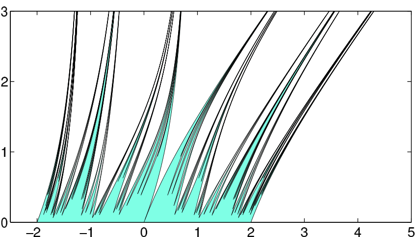
Figure 5 depicts the covers $\Sigma_{k}^{\sf a}\cup\Sigma_{k}^{\sf b}$ for the period doubling potential and $\Sigma_{k}^{\sf a}\cup\Sigma_{k+1}^{\sf a}$ for Thue–Morse as $\lambda$ increases from zero with $k=7$, giving an impression of how rapidly the covering intervals shrink as $\lambda$ increases. Notice the quite different nature of the spectra obtained from these two substitution rules. Similar figures for the Fibonacci spectrum are shown in [14]. (The algorithm described in the last section enables such computations for much larger values of $k$, but the resulting figures become increasingly difficult to render due to the number and narrow width of the covering intervals.)

High fidelity spectral approximations for quasiperiodic Schrödinger operators are tricky to compute due not only to the complexity of the eigenvalue problem, but also considerations of numerical precision. The LAPACK symmetric eigenvalue algorithms are expected to compute eigenvalues of the $K\times K$ matrix ${\bf J}_{\pm}$ accurate to within $p(K)\|{\bf J}_{\pm}\|\varepsilon_{\rm mach}$ [2, p. 104], where $p(K)$ is a “modestly growing function of $K$” and $\varepsilon_{\rm mach}$ denotes the machine epsilon value for the floating point arithmetic system (on the order of $10^{-16}$ for double precision and $10^{-34}$ for quadruple precision [1]). Figure 6 shows the width of the smallest interval in the approximation $\Sigma_{k}^{\sf a}$ for the period doubling and Thue–Morse potentials, as computed in double and quadruple precision arithmetic for various values of $\lambda$. As $\lambda$ increases, this smallest interval shrinks ever quicker. Comparing double and quadruple precision values, one sees that for even moderate values of $K=2^{k}$, double precision is unable to accurately resolve the spectrum.⁸⁸ 8 The calculations of fractal dimension and gaps that follow were performed in quadruple precision arithmetic, and we generally restricted the values of $\lambda$ and $k$ to obtain numerically reliable results. In the event the numerical results violate the ordering of eigenvalues of ${\bf J}_{+}$ and ${\bf J}_{-}$ in (1.8), any offending interval is replaced by one of width $20\kern 1.0pt\varepsilon_{\rm mach}$ centered at the midpoint of the computed eigenvalues. (Similar numerical errors will be observed for the original matrix ${\bf J}_{\pm}$. Since it only permutes matrix entries, our algorithm does not introduce any new instabilities.)

The quasiperiodic spectrum $\Sigma$ is known to be a Cantor set for the Fibonacci, period doubling, and Thue–Morse potentials for all $\lambda>0$, suggesting calculation of the fractal dimensions of these sets as functions of $\lambda$. We begin with two standard definitions; see, e.g., [22, 37].

The analysis in the last section provides natural covering sets for $\Sigma$, which we denote as $C_{k}$ (i.e., for period doubling, $C_{k}\equiv\Sigma_{k}^{\sf a}\cup\Sigma_{k}^{\sf b}$; for Fibonacci and Thue–Morse, $C_{k}\equiv\Sigma_{k}^{\sf a}\cup\Sigma_{k+1}^{\sf a}$). We estimate $\dim_{H}(\Sigma)$ using a heuristic proposed by Halsey et al. [24]. Enumerate the $n_{k}$ intervals in $C_{k}$ as $\{B_{k,m}\}$:

For the Fibonacci case, Damanik et al. [15] proved upper and lower bounds on $\dim_{H}(\Sigma)$ for $\lambda\geq 8$ in terms of the functions $S_{u}(\lambda)=2\lambda+22$ and $S_{l}(\lambda)=\frac{1}{2}\big(\lambda-4+\sqrt{(\lambda-4)^{2}-12}\big)$. To benchmark our method, we compare the approximate dimension with the upper and lower bounds, as shown in Figure 7, indeed obtaining satisfactory results. Figure 8 shows estimates to $\dim_{H}(\Sigma)$ drawn from spectral covers for $k=6,\ldots,10$, with good convergence in $k$ in the small $\lambda$ regime. The narrow covering intervals for large $\lambda$ and $k$ pose a significant numerical challenge, even in quadruple precision arithmetic.

The bounds from [15] imply $\dim_{H}(\Sigma)\to 0$ like $\log(1+\sqrt{2})/\log(\lambda)$ as $\lambda\to\infty$ for the Fibonacci case. In contrast, Liu and Qu [32] recently showed that for the Thue–Morse operator, $\dim_{H}(\Sigma)$ is bounded away from zero as $\lambda\to\infty$. Interestingly, the approximation scheme described above does not yield consistent results for Thue–Morse, perhaps a reflection of the exotic behavior identified in [32]. As an alternative, in Figure 9 we show estimates of the box-counting dimension for Thue–Morse. Since for any finite $k$ the covers comprise the finite union of real intervals, $\log(N_{C_{k}}(\varepsilon))/\log(1/\varepsilon)\to 1$ as $\varepsilon\to 0$. However, for finite $\varepsilon$ the shape of the curves in Figure 9 can suggest rough values for ${\rm dim}_{B}(\Sigma)$; cf. [45]. Figure 10 repeats the experiment for period doubling; note that the plot for $\lambda=4$ shows good agreement with the estimate for $\dim_{H}(\Sigma)$ seen in Figure 8. (The Hausdorff and box counting dimensions need not be equal; considerable effort was devoted over the years to showing $\dim_{H}(\Sigma)={\rm dim}_{B}(\Sigma)$ for all $\lambda>0$ for the Fibonacci case, with the complete result obtained only recently [19].)

The spectral covers we have described can behave in rather subtle ways. To illustrate this fact, Figure 11 shows the largest gap in the Thue–Morse cover $\Sigma_{k}^{\sf a}\cup\Sigma_{k+1}^{\sf a}$ as a function of the parameter $\lambda$. Bellisard [7] showed that, for the aperiodic model, this gap should behave like $\lambda^{\log 4/\log 3}$ as $\lambda\to 0$. The covers satisfy this characterization for intermediate values of $\lambda$, but appear to behave instead like $\lambda^{2}$ as $\lambda\to 0$. The larger the value of $k$ (hence the longer the periodic approximations), the larger the range of $\lambda$ values that are consistent with Bellisard’s spectral asymptotics. This scenario provides another justification for the study of large-$k$ approximations: for this potential, one must consider large $k$ to approximate the spectrum adequately for small $\lambda$.

Our algorithm also expedites study of the square Hamiltonians $\mbox{\boldmath$\mathcal{J}$}_{\rm sq}$ acting on $\ell^{2}({\mathbbm{Z}})\times\ell^{2}({\mathbbm{Z}})$ via

The spectrum of this operator is $\Sigma+\Sigma$, where $\Sigma$ is the spectrum of the standard 1-dimensional operator with potential $\{b_{n}\}$. When $\Sigma$ is a Cantor set, $\Sigma+\Sigma$ could be an interval, a union of intervals, a Cantorval, or a Cantor set; see, e.g., [34, 35, 37]. For further details and examples for the Fibonacci case, see [14] and the computations, based on $\sigma({\bf J}_{\pm})$, of Even-Dar Mandel and Lifshitz [21]. For the period doubling and Thue–Morse potentials, Figure 12 illustrates how the covers of the spectra for these square Hamiltonians develop in $\lambda$, revealing values of $\lambda$ for which $\Sigma+\Sigma$ cannot comprise a single interval.

We thank a referee for helpful comments that led us to study the largest Thue–Morse gap (Figure 11), and David Damanik, Paul Munger, Beresford Parlett, and Dan Sorensen for fruitful discussions. We especially thank May Mei for suggesting computations with substitution operators and sharing numerical results, and Adrian Forster for his Thue–Morse computations.

References

- [1] IEEE Standard for Floating-Point Arithmetic (IEEE Standard 754–2008). Institute of Electrical and Electronics Engineers, Inc., 2008.
- [2] E. Anderson, Z. Bai, C. Bischof, S. Blackford, J. Demmel, J. Dongarra, J. Du Croz, A. Greenbaum, S. Hammarling, A. McKenney, and D. Sorensen. LAPACK User’s Guide. SIAM, Philadelphia, third edition, 1999.
- [3] A. Avila and S. Jitomirskaya. The ten martini problem. Ann. of Math., 170:303–342, 2009.
- [4] A. Avila and R. Krikorian. Reducibility or nonuniform hyperbolicity for quasiperiodic Schrödinger cocycles. Ann. of Math., 164:911–940, 2006.
- [5] Y. Avishai and D. Berend. Trace maps for arbitrary substitution sequences. J. Phys. A, 26:2437–2443, 1993.
- [6] Y. Avishai, D. Berend, and D. Glaubman. Minimum-dimension trace maps for substitution sequences. Phys. Rev. Lett., 72:1842–1845, 1994.
- [7] J. Bellissard. Spectral properties of Schrödinger’s operator with a Thue–Morse potential. In Number Theory and Physics, volume 47 of Springer Proceedings in Physics, pages 140–150. Springer-Verlag, Berlin, 1990.
- [8] J. Bellissard, B. Iochum, E. Scoppola, and D. Testard. Spectral properties of one-dimensional quasicrystals. Comm. Math. Phys., 125:527–543, 1989.
- [9] Jean Bellissard, Anton Bovier, and Jean-Michel Ghez. Spectral properties of a tight binding Hamiltonian with period doubling potential. Comm. Math. Phys., 135:379–399, 1991.
- [10] Christian H. Bischof, Bruno Lang, and Xiaobai Sun. A framework for symmetric band reduction. ACM Trans. Math. Software, 26:581–601, 2000.
- [11] D. Damanik. Singular continuous spectrum for a class of substitution Hamiltonians II. Lett. Math. Phys., 54:25–31, 2000.
- [12] D. Damanik. Uniform singular continuous spectrum for the period doubling Hamiltonian. Ann. Henri Poincaré, 2:101–118, 2001.
- [13] D. Damanik. Strictly ergodic subshifts and associated operators. In Spectral Theory and Mathematical Physics: a Festschrift in Honor of Barry Simon’s 60th Birthday, volume 76 of Proc. Sympos. Pure Math., pages 539–563. American Mathematical Society, Providence, RI, 2007.
- [14] D. Damanik, M. Embree, and A. Gorodetski. Spectral properties of Schrödinger operators arising in the study of quasicrystals, 2012. arXiv:1210.5753 [math.SP].
- [15] D. Damanik, M. Embree, A. Gorodetski, and S. Tcheremchantsev. The fractal dimension of the spectrum of the Fibonacci Hamiltonian. Comm. Math. Phys., 280:499–516, 2008.
- [16] D. Damanik and A. Gorodetski. Almost sure frequency independence of the dimension of the spectrum of Sturmian Hamiltonians, 2014. arXiv:1406.4810 [math.SP].
- [17] D. Damanik and D. Lenz. Uniform spectral properties of one-dimensional quasicrystals, I. Absence of eigenvalues. Comm. Math. Phys., 207:687–696, 1999.
- [18] David Damanik and Jake Fillman. Spectral Theory of Discrete One-Dimensional Ergodic Schrödinger Operators. In preparation.
- [19] David Damanik, Anton Gorodetski, and William Yessen. The Fibonacci Hamiltonian, 2014. arxiv:1403.7823 [math.SP].
- [20] F. Delyon and J. Peyrière. Recurrence of the eigenstates of a Schrödinger operator with automatic potential. J. Stat. Phys., 64:363–368, 1991.
- [21] S. Even-Dar Mandel and R. Lifshitz. Electronic energy spectra of square and cubic Fibonacci quasicrystals. Phil. Mag., 88:2261–2273, 2008.
- [22] Kenneth Falconer. Fractal Geometry: Mathematical Foundations and Applications. Wiley, Chichester, 2nd edition, 2003.
- [23] C. W. Gear. A simple set of test matrices for eigenvalue programs. Math. Comp., 23:119–125, 1969.
- [24] Thomas C. Halsey, Mogens H. Jensen, Leo P. Kadanoff, Itamar Procaccia, and Boris I. Shraiman. Fractal measures and their singularities: the characterization of strange sets. Phys. Rev. A, 33:1141–1151, 1986.
- [25] P. G. Harper. Single band motion of conduction electrons in a uniform magnetic field. Proc. Phys. Soc. A, 68:874–878, 1955.
- [26] A. Hof, O. Knill, and B. Simon. Singular continuous spectrum for palindromic Schrödinger operators. Comm. Math. Phys., 174:149–159, 1995.
- [27] Mahito Kohmoto, Leo P. Kadanoff, and Chao Tang. Localization problem in one dimension: mapping and escape. Phys. Rev. Lett., 50:1870–1872, 1983.
- [28] S. Kotani. Jacobi matrices with random potentials taking finitely many values. Rev. Math. Phys., 1:129–133, 1989.
- [29] Michael P. Lamoureux. Reflections on the almost Mathieu operator. Integral Equations Operator Theory, 28:45–59, 1997.
- [30] Y. Last. Zero measure spectrum for the almost Mathieu operator. Comm. Math. Phys., 164:421–432, 1994.
- [31] Yoram Last. Quantum dynamics and decompositions of singular continuous spectra. J. Funct. Anal., 142:406–445, 1996.
- [32] Qinghui Liu and Yanhui Qu. Iteration of polynomial pair under Thue–Morse dynamic, 2014. arXiv:1403.2257 [math.DS].
- [33] Laurent Marin. On- and off-diagonal Sturmian operators: Dynamic and spectral dimension. Rev. Math. Phys., 24(05):1250011, 2012.
- [34] Pedro Mendes and Fernando Oliveira. On the topological structure of the arithmetic sum of two Cantor sets. Nonlinearity, 7:329–343, 1994.
- [35] Carlos G. Moreira, Eduardo Muñoz Morales, and Juan Rivera-Letelier. On the topology of arithmetic sums of regular Cantor sets. Nonlinearity, 13:2077–2087, 2000.
- [36] Stellan Ostlund, Rahul Pandit, David Rand, Hans Joachim Schellnhuber, and Eric D. Siggia. One-dimensional Schrödinger equation with an almost periodic potential. Phys. Rev. Lett., 50:1873–1876, 1983.
- [37] Jacob Palis and Floris Takens. Hyperbolicity and Sensitive Chaotic Dynamics at Homoclinic Bifurcations. Cambridge University Press, Cambridge, 1993.
- [38] Beresford N. Parlett. The Symmetric Eigenvalue Problem. SIAM, Philadelphia, SIAM Classics edition, 1998.
- [39] M. Queffélec. Substitution Dynamical Systems – Spectral Analysis. Springer, Berlin, 1987.
- [40] Michael Reed and Barry Simon. Methods of Modern Mathematical Physics I: Functional Analysis. Academic Press, San Diego, revised and enlarged edition, 1980.
- [41] W. Rudin. Some theorems on Fourier coefficients. Proc. Amer. Math. Soc., 10:855–859, 1959.
- [42] H. Rutishauser. On Jacobi rotation patterns. In Experimental Arithmetic, High Speed Computing and Mathematics, volume 15 of Proceedings of Symposia in Applied Mathematics, pages 219–239. American Mathematical Society, Providence, RI, 1963.
- [43] H. S. Shapiro. Extremal problems for polynomials and power series. Master’s thesis, Massachusetts Institute of Technology, 1951.
- [44] Barry Simon. Szegő’s Theorem and Its Descendants. Princeton University Press, Princeton, NJ, 2011.
- [45] Tamás Tél, Ágnes Fülöp, and Tamás Vicsek. Determination of fractal dimensions for geometrical multifractals. Physica A, 159:155–166, 1989.
- [46] Gerald Teschl. Jacobi Operators and Completely Integrable Nonlinear Lattices. American Mathematical Society, Providence, RI, 2000.
- [47] D. J. Thouless. Bandwidths for a quasiperiodic tight-binding model. Phys. Rev. B, 28:4272–4276, 1983.
- [48] Morikazu Toda. Theory of Nonlinear Lattices. Springer-Verlag, Berlin, 2nd edition, 1989.
- [49] Pierre van Moerbeke. The spectrum of Jacobi matrices. Inv. Math., 37:45–81, 1976.
- [50] W.N. Yessen. Spectral analysis of tridiagonal Fibonacci Hamiltonians. J. Spectral Theory, 3:101–128, 2013.