Analysis of Recurrent Linear Networks for Enabling Compressed Sensing of Time-Varying Signals
Abstract
Recent interest has developed around the problem of dynamic compressed sensing, or the recovery of time-varying, sparse signals from limited observations. In this paper, we study how the dynamics of recurrent networks, formulated as general dynamical systems, mediate the recoverability of such signals. We specifically consider the problem of recovering a high-dimensional network input, over time, from observation of only a subset of the network states (i.e., the network output). Our goal is to ascertain how the network dynamics lead to performance advantages, particularly in scenarios where both the input and output are corrupted by disturbance and noise, respectively. For this scenario, we develop bounds on the recovery performance in terms of the dynamics. Conditions for exact recovery in the absence of noise are also formulated. Through several examples, we use the results to highlight how different network characteristics may trade off toward enabling dynamic compressed sensing and how such tradeoffs may manifest naturally in certain classes of neuronal networks.
Index Terms:
Recurrent networks, linear dynamic systems, over-actuated systems, sparse input, minimizationI Introduction
We consider the analysis of recurrent networks for facilitating recovery of a high-dimensional, time-varying, sparse input in the presence of both corrupting disturbance and confounding noise. The network receives an input and generates the observations (network outputs), via its recurrent dynamics, i.e.,
where, here, are the network states, is the corrupting disturbance and is the confounding noise. Our focus is on how the network dynamics, embedded in , impact the extent to which can be inferred from in the case where the dimensionality of the latter is substantially less than that of the former. We will focus exclusively on the case where these dynamics are linear.
Such a problem, naturally, falls into the category of sparse signal recovery or compressed sensing (CS), for under-determined linear systems [1, 2, 3]. It is well known that for such problems, exact and stable recovery can be achieved under certain assumptions related to the statistical properties of the observed signal [4, 5, 6, 7]. Classical CS, however, does not typically consider temporal dynamics associated with the recovery problem.
I-A Motivation
Given the natural sparsity of electrical signals in the brain, CS has been linked to important questions in neural decoding [8, 9], i.e., how the brain represents and transforms information. Understanding the dynamics of brain networks in the context of CS is a crucial aspect of this overall problem [10, 8, 11, 12]. Such networks are, of course, not static. Thus, recent interest has grown around so-called dynamic CS and, specifically, on the recovery of signals subjected to transformation via a dynamical system (or, network). In this context, sparsity has been formulated in three ways: 1) In the network states (state sparsity) [13, 14, 15]; 2) In the structure/parameters of the network model (model sparsity) [16, 17]; and 3) In the inputs to the network (input sparsity) [18, 19, 20, 21, 22, 23, 24, 25, 26, 27, 28]. Here, we consider this latter category of recovery problems.
Our motivation is to understand how three stages of a generic network architecture – an afferent stage, a recurrent stage, and an output stage (see Fig. 1) – interplay in order to enable an observer, sampling the output, to recover the (sparse) input. Such an architecture is pervasive in sensory networks in the brain wherein a large number of sensory neurons, receiving excitation from the periphery, impinge on an early recurrent network layer that transforms the afferent excitation en route to higher brain regions [29, 30]. Moreover, beyond neural contexts, understanding network characteristics for dynamic CS may aid in the analysis of systems for efficient processing of naturally sparse time-varying signals [20]; and in the design of resilient cyber-physical systems [18, 19, 21], wherein extrinsic perturbations are sparse and time-varying. Toward these potential instantiations, our specific aim in this paper is to elucidate fundamental dynamical characteristics of linear networks for exact and stable recovery of the (sparse) input signal, corrupted by an input disturbance.

I-B Paper Contributions
To achieve our specific aim, we develop and present the following contributions:
- 1.
We develop analytical conditions on the network dynamics, related to the classical notion of observability for a linear system, such that the network admits exact and stable (in the presence of output noise) input recovery.
- 2.
We derive an upper bound in terms of the network dynamics, for the -norm of the reconstruction error over a finite time horizon. This error can be defined in terms of both the disturbance and the noise.
- 3.
Based on the error analysis, we characterize a basic tradeoff between the ability of a network to simultaneously reject input disturbances while still admitting stable recovery.
- 4.
We highlight network characteristics that optimally balance this tradeoff, and demonstrate via several examples their ability to reconstruct corrupted time-varying input from noisy observations. In particular, we highlight an example of a rate-based neuronal network, and how specific features of the network architecture mediate these tradeoffs.
I-C Prior Results in Sparse Input Recovery
The sparse input recovery problem for linear systems can be formulated in both the spatial and temporal dimension. Our contributions are related to the former. As mentioned above, in this context, previous work has considered recovery of spatially sparse inputs for network resilience [18, 19] and encoding of inputs with sparse increments [20]. In [21], conditions for exact sparse recovery are formulated in terms of a coherence-based observability criterion for intended applications in cyber-physical systems. Our contributions herein provide a general set of analytical results, including performance bounds, pertaining to exact and stable sparse input recovery of linear systems in the presence of both noise and disturbance.
A second significant line of research in sparse input recovery problems pertains to the temporal dimension. There, the goal is to understand how a temporally sparse signal (i.e., one that takes the value of zero over a nontrivial portion of its history) can be recovered from the state of the network at a particular instant in time. This problem forms the underpinning of a characterization of ‘memory’ in dynamical models of brain networks [22, 23, 24, 25, 26, 27]. In particular, in [28] the problem of ascertaining memory is related to CS performed on the network states, over a receding horizon of a scalar-valued input signal. In contrast to these works, we consider spatial sparsity of vector-valued inputs with explicit regard for both disturbance and an overt observation equation, i.e., states are not be directly sampled, but are transformed to an (in general lower-dimensional) output.
I-D Paper Outline
The remainder of the paper is organized as follows. In Section II we provide motivation of the current work and formulate the problem in detail. In Section III we develop theoretical results on the performance of the proposed recovery method. Simulation results for several different scenarios are provided in Section IV. Finally, conclusions are formulated in Section V.
II Problem Formulation
We consider a discrete-time model for a linear network, formulated in the typical form a linear dynamical system, i.e.,:
| (1) | ||||
where is an integer time index, is the activity of the network nodes (e.g., in the case of a rate-based neuronal network [31, 32, 33, 34, 35, 36, 37], the firing rate of each neuron), is the extrinsic input, is the input disturbance, is the measurement noise independent from , and is the observation at time . The matrix describes connections between nodes in the network, contains weights between input and output and is the measurement matrix. Such a model is, of course, quite general and can be used to describe recurrent dynamics in neuronal networks [38, 39, 40, 41, 42], machine learning applications such as pattern recognition and data mining [43, 44, 45, 46], etc.
We consider the case of bounded disturbance and noise, i.e., , . Since , the number of input nodes, is larger than , the number of output nodes, takes the form of a “wide” matrix. We assume that at each time at most input nodes are active (-sparse input), leading to an constraint to (1) at each time point:
| (2) |
In the absence of disturbance and noise, recovering the input of (1) with the constraint (2) amounts to the optimization problem:
| (3) | ||||||||
It is clear that Problem () is a non-convex discontinuous problem, which is not numerically feasible and is NP-Hard in general [47]. For static cases, such optimization problems fall into the category of combinatorial optimization which require exhaustive search to find the solution [48].
Thus, throughout this paper, we follow the typical relaxation methodology used for such problems wherein the norm is relaxed to the norm, resulting in the problem:
| (4) | ||||||||
In the case that either input disturbance, or measurement noise, or both exist, we solve the following convex optimization Problem ():
| (5) | ||||||||
where is 2-norm of a surrogate parameter that aggregates the effects of disturbance and noise. In the case of noisy measurement with no disturbance . In the next section, we show conditions for the network (1) under which Problems () and () result in exact and stable solutions.
III Results
We will develop our results in several steps. First, we consider two cases for the observation matrix in the absence of input disturbance, and proceed to establish existence and performance guarantees for solutions to the convex problems () and () for each case. After that, we continue the analysis to characterize the ability of a network to reject input disturbances while still admitting stable recovery in the presence of disturbance and noise, simultaneously.
III-A Preliminaries
We begin by recalling some basic matrix notation and matrix norm properties that will be used throughout this paper. Given normed spaces and , the corresponding induced norm or operator norm denoted by over linear maps , is defined by
| (6) | ||||
where is the set of eigenvalues of (or the spectrum of ).
Definition 1:
A vector is said to be -sparse if , in other words it has at most nonzero entries.
It is well known that in the static case (standard CS), exact and stable recovery of sparse inputs can be obtained under the restricted isometry property (RIP) [4, 5, 6, 7, 49], defined as:
Definition 2:
The restricted isometry constant of a matrix is defined as the smallest number such that for all -sparse vectors the following equation holds
| (7) |
III-B Case 1: Full-rank Square Observation Matrix without Input Disturbance
In the first case, we consider (1) in the absence of input disturbance () and we assume that the linear map , , has no nullspace, , which means that the network states can be exactly recovered by inverting the observation equation (1) (the trivial case being C equal to the identity). Our first result establishes a one to one correspondence between sparse input and observed output for the system (1).
Lemma 3:
Suppose that the sequence from noiseless measurements is given, and , , , are known. Assume the matrix satisfies the RIP condition (7) with isometry constant . Then, there is a unique -sparse sequence of and a unique sequence of that generate .
Proof.
See Appendix A. ∎
Having established the existence of a unique solution, we now proceed to study convex Problems () and () that recover these solutions. First, we provide theoretical results for the stable recovery of the input where measurements are noisy i.e., ().
Theorem 4:
(Noisy recovery) Assume that the matrix satisfies the RIP condition (7) with . Suppose that the sequence is given and generated from sequences and -sparse based on
| (8) | ||||
where and , , , are known. Then, the solution to Problem () obeys
| (9) |
where
| (10) |
are given explicitly below:
| (11) | ||||
Proof.
Assume that the the sequences and sparse are the solutions of Problem (). First we derive the bound for the in the following Lemma.
Lemma 5:
Suppose that the sequence is given and generated from sequences and -sparse based on (8), where and , , , are known. Then, any solution to Problem () obeys
| (12) |
Proof.
See Appendix B ∎
From Lemma 12, non-singularity of and the equation we can derive a bound for as
| (13) | ||||
which results in
| (14) |
Now, denote where can be decomposed into a sum of vectors for each , each of sparsity at most . Here, corresponds to the location of non-zero elements of , to the location of largest coefficients of , to the location of the next largest coefficients of , and so on. Also, let . Extending the technique in [7, 49], it is possible to obtain a cone constraint for the input in the linear dynamical systems.
Lemma 6:
(Cone constraint) The optimal solution for the input in Problem () satisfies
| (15) |
Proof.
See Appendix C. ∎
We can further establish a bound for the right hand side of (15):
Lemma 7:
The optimal solution for the input in Problem () satisfies the following constraint
| (16) |
Proof.
See Appendix D. ∎
We now state a Theorem that characterizes the solution for the noiseless case (P1), which follows as a special case of (P2) as the noise variance approaches zero.
Theorem 8:
III-C Case 2: Observation Matrix Satisfying Observability Condition without Input Disturbance
In this case, we consider (1) in the absence of input disturbance () with the linear map , . Thus, direct inversion of is not possible in this case. For any positive , we define the standard linear observability matrix as
| (18) |
If , then the system (1) is observable in the classical sense 11 1 The system is said to be observable if, for any initial state and for any known sequence of input there is a positive integer such that the initial state can be recovered from the outputs , ,…, . . However, we do not assume any knowledge of the input other than the fact that it is -sparse at each time. Note that if we simply iterate the output equation in (1) for time steps and exploit the fact that the input vector is -sparse as shown in Fig. 2, we obtain:
| (19) |
where is as follows:
| (20) |
where is the matrix corresponding the active columns of (corresponding to nonzero input entries) at time step (see Fig. 2). In general, we do not know where active columns of are located at each time a priori. We define as the set of all possible matrices satisfying the structure in (20), where the cardinality of this set is .

In the next Theorem, we establish conditions under which a one to one correspondence exists between sparse input and observed output for the system (1).
Lemma 9:
Suppose that the sequence from noiseless measurements is given, and , and are known. Assume and the matrix satisfies the RIP condition (7) with isometry constant . Further, assume
| (21) |
Then, there is a unique -sparse sequence of and a unique sequence of that generate .
Proof.
See Appendix E. ∎
Remark 10:
The rank condition implies that all columns of the observability matrix must be linearly independent of each other (i.e., the network is observable in the classical sense) and of all columns of . Since the exact location of the nonzero elements of the input vector are not known a priori, this condition is specified over all . Thus, (21) is a combinatorial condition. From our simulation studies, we observe that this condition holds for random Gaussian matrices almost always and, moreover, can be numerically verified for certain salient random networks (see also Example 3 in Section IV).
Having established the existence of a unique solution, we now proceed to study the convex problems () and () that recover these solutions for this case. First, we provide theoretical results for the stable recovery of the input where measurements are noisy i.e., (P2).
Theorem 11:
Proof.
See Appendix F. ∎
Theorem 12:
(Noiseless recovery) Assume and the matrix satisfies the RIP condition (7) with . Further, assume (21) holds. Suppose that the sequence is given and generated from sequences and -sparse inputs based on dynamical equation (8), where and , and are known. Then the sequences and are the unique minimizer to Problem ().
Proof.
Remark 13:
Imposing an RIP condition on the combined matrix bears some conceptual similarity to the formulation of an overcomplete dictionary in the classical compressed sensing literature [53, 54]. In this sense, the matrix (i.e., the afferent stage) can be interpreted as a dictionary that transforms the sparse input onto the recurrent network states.
III-D Case 3: Optimal Network Design to Enable Recovery in the Presence of Disturbance and Noise
Finally, we show how eigenstructure of the network implies a fundamental tradeoff between stable recovery and rejection of disturbance (i.e., corruption).
It is easy to see from (9) that the upper-bound of the recovery error is reduced by decreasing the maximum singular value of . Thus, from now on we use the upper-bound of the input recovery error as a comparative measure of performance. In the absence of both disturbance and noise, the best error performance is achieved when , i.e., the network is static, which in intuitive since in this scenario any temporal effects would smear the salient parts of the signal.
On the other hand, having dynamics in the network should improve the error performance in the presence of the disturbance. To demonstrate this, consider (1) with nonzero. When , i.e., a static network, the disturbance can be exactly transformed to the measurement equation resulting in as a surrogate measurement noise with
| (23) | ||||
In this case, the error upper-bound can be obtained by exploiting the result of Theorem 4 as
| (24) | ||||
When is nonzero, it is not possible to exactly map the disturbance to the output as above. Nevertheless, it is straightforward to approximate the relative improvement in performance. For instance, consider a system with symmetric and where the disturbance and input are in displaced frequency bands. Then it is a direct consequence of linear filtering that the power spectral density of the disturbance can be attenuated according to
| (25) |
where is the frequency of the disturbance. So, for instance, if ,
| (26) | ||||
where is the eigenvalue of matrix . Assuming the input is sufficiently displaced in frequency from the disturbance, the error upper-bound can be then readily approximated using the results of Theorem 4 as follows
| (27) | ||||
By comparing (24) and (27), it is easy to verify that A and C can be designed in a way to reduce error upper-bound at least by a factor of two, assuming and are close to each other. In the examples below, we will show that, in fact, performance in many cases can exceed this bound considerably.
IV Examples
In this section, we present several examples that demonstrate the developed results. For solving our convex optimization problems, we used CVX with MATLAB interface [55, 56]. To create example networks, we generated the matrices , , using a Gaussian random number generator in MATLAB.
IV-A Example 1: One-step and Sequential Recovery
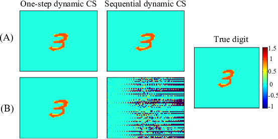
In this experiment, we consider a dynamical system with sparse input which satisfies conditions in Theorem 22. Here, we consider random Gaussian matrices for , and , with , . The input is defined as the image of a digit, shown in Fig. 3 with values between 0 and 1, where the horizontal axis is treated as time, i.e., column of the image is the input to the system at time .
We proceed to perform input recovery in two ways: (i) by solving () in one step over the entire horizon , i.e., one-step recovery; and (ii) by solving () times, sequentially, i.e., recovery at each time step. We compare the outcomes for two cases:
Full Rank
Fig. 3A shows the recovered input for the case that for both one-step and sequential recovery, and it can be seen that sparse input can be recovered in two cases perfectly. This is expected, since in this case, can be inverted at each time step.
Satisfying Observability Condition
Fig. 3B of the figure illustrates the results for the case that , but where satisfies the observability condition. It is clear that sequential dynamic CS can not recover the input exactly. However, from our results (Theorem 12) we expect that one-step recovery (over the entire horizon) is possible, as is evidenced in the figure.
IV-B Example 2: Recovery in the Presence of Disturbance and Noise
Fig. 4A shows the mean square error () versus the maximum singular value of , for several random realization of , in the case of full rank . In this study, is assumed to follow an uniform distribution while . It can be seen from this figure that by increasing , the recovery performance is degraded, as we expect based on the derived bound for the error in (9).

To contrast Fig. 4A, we consider the case when disturbance is added to the input. In Fig. 4B, we show the versus for several random diagonal matrices when and . As expected from our results, can not be arbitrary small, since in this case the disturbance would entirely corrupt the input.
We conducted simulation experiments to examine the effect of the noise and disturbance strength on the reconstruction error. Fig. 5 shows the average for the reconstructed input versus and , respectively with , for random trials (different random matrices A, B, C in each trial). This figure shows that the reconstruction error decreases as a function of noise energy.


The next study illustrates recovery in the presence of both disturbance and noise for a smoothly changing sequence of 64 images (frames). Each frame, is corrupted with disturbance and at each time, and the difference between two consecutive frames is considered as the sparse input to the network. The disturbance is assumed to be a random variable drown from a Gaussian distribution, , passed through a fifth-order Chebyshev high pass filter. Each frame has pixels and . Furthermore, we consider random Gaussian matrices for and with .
We proceeded to design the matrix to balance the performance bound (9) and the ability to reject the disturbance as per Section III-D. Fig. 6A shows the original frames at different times. We assumed the first frame is known exactly. Frames recovered from the output of a static network , i.e., are depicted in Fig. 6B. In contrast, frames recovered from the output of the designed dynamic network are shown in Fig. 6C. It is clear from the figure that quality of recovery is better in the latter case. Fig. 7 illustrates the PSNR, defined as as a function of frame number with and without dynamics. It can be concluded from this figure that having a designed matrix results in recovery that is more robust to disturbance, while without dynamics, error propagates over time, and the reconstruction quality is degraded.

IV-C Example 3: Input Recovery in an Overactuated Rate-Based Neuronal Network
A fundamental question in theoretical neuroscience centers on how the architecture of brain networks enables the encoding/decoding of sensory information [57, 10]. In our final example, we use the results of Theorems 4 and 12 to highlight how certain structural and dynamical features of neuronal networks may provide the substrate for sparse input decoding.
Specifically, we consider a firing rate-based neuronal network [34] of the form
| (28) |
with input rates , output rates , a feed-forward synaptic weight matrix , and a recurrent synaptic weight matrix . We consider neurons which receive synaptic inputs from afferent neurons, i.e., neurons that impinge on the network in question. Here, is a diagonal matrix whose diagonal elements are the time constants of the neurons. A discrete version of (28), alongside a linear measurement equation can be written in the standard form (1) where is related to connections between nodes in the network, and contains weights between input and output nodes. For this example, we assume that the network connectivity has a Watts–Strogatz small-world topology [58] with connection probability and rewiring probability .
The recurrent synaptic matrix is defined as
| (29) |

For the purposes of illustration, we select the diagonal elements of matrix , from a uniform distribution . We study the recovery performance associated with the network over 100 time steps, assuming a timescale of milliseconds and an discretization step of . At each time step, the nonzero elements of the input vector , i.e., firing rate of the afferent neurons, are drawn from an uniform distribution . Moreover, we assume that elements of the observation matrix are drawn from a Gaussian distribution . Finally, we assume and are drawn from lognormal distributions and , respectively. The latter assumption is chosen for illustration only and is not related to known physiology.
IV-C1 Recovery Performance from Error Bounds
We proceed to conduct a Monte Carlo simulation of 100 different realizations of , and . Fig. 8A illustrates that the maximum singular value of the matrix decreases as a function of the percent of inhibitory neurons. Thus, we anticipate from our derived performance bounds that performance in terms of mean square error (MSE) should be best for networks with high inhibition in the presence of noise. This prediction bears out in Fig. 8B, where we indeed observe a monotone relationship between MSE and inhibition. On the one hand, low-inhibition is favorable for facilitating recovery in the presence of disturbance depicted in Fig. 8C. Such tradeoffs are interesting to contemplate when considering the functional advantages of network architectures observed in biology, such as the pervasive 80-20 ratio of excitatory to inhibitory neurons [34, 59]. Together, Figs. 8B and 8C illustrate how the excitatory-inhibitory ratio mediate a basic tradeoff in the capabilities of a rate-based neuronal network.
IV-C2 Recoverable Sparsity based on Theorem 12
Having ascertained the performance tradeoff curves, we sought to characterize in more detail the level of recoverable sparsity with specific connection to Theorem 12 and (21). We considered networks as above, but with and 20/80 for the ratio of inhibitory/excitatory over 10 time steps for 100 random trials. Thus, the output of the network is of lower dimension than the network state space and the observability matrix is of nontrivial construction. Fig. 9A shows that for this setup, the rank condition (21) holds up to . Thus, Theorem 12 predicts that recover will be possible (to within the RIP condition on ) for signals with 13 nonzero elements. Fig. 9B validates this theoretical prediction by illustrating recovery performance in the absence of disturbance and noise for different values . It is observed that when the rank condition holds, reconstruction is perfect and that the probability of exact recovery is decreased by increasing , as expected.

V Conclusion
V-A Summary
In this paper, we present several results pertaining to the effect of temporal dynamics on compressed sensing of time-varying signals. Specifically, we considered the recovery of sparse inputs to a linear dynamical system (network) from limited observation of the network states. We provide basic conditions on the system that ensure solution existence and, further, derive several bounds in terms of the system dynamics for recovery performance in the presence of both input disturbance and observation noise. We show that dynamics can play opposing roles in mediating accurate recovery with respect to these two different sources of corruption. Thus, our results indicate tradeoffs that may inform the design of dynamical systems for time-varying compressed sensing. These tradeoffs are illustrated through a series of examples, including one that highlights how the developed theory could be used to interrogate the functional role of inhibition in a neuronal network.
V-B Implications and Future Work
The results can have both engineering and scientific impacts. In the former case, the goal may be to design networks to process time-varying signals that are naturally sparse, such as high-dimensional neural data, or to be resilient to time-varying sparse perturbations. In the latter case, the goal is to understand how the naturally occurring architectures of networks, such as those in the brain, confer advantages for processing of afferent signals. In both cases, a precursor to further study are a set of verifiable conditions that overtly link network characteristics/dynamics to sparse input processing. Our paper provides such conditions for networks with linear dynamics and develops illustrative examples that highlight these potential applications. Treatment of systems with nonlinear dynamics, as well as a more detailed examination of random networks using the theory, are left as subjects for future work.
Appendix A Proof of Lemma 3
Based on the assumption on the null space of the linear map , given , there is a unique sequence of . We now prove the uniqueness of . First, consider the following equations:
| (30) | ||||
The remainder of the proof is by contradiction. Let us assume that the sequence is not unique and there is another sequence of -sparse which satisfies (30), leading to
| (31) | ||||
Therefore, based on (30) and (31) we can conclude that
| (32) |
Matrix is non-singular, hence equation (33) can be simplified as follows:
| (33) |
Based on the assumption that the matrix satisfies the RIP condition (7) with isometry constant and the fact that the support of the vectors are at most , the lower bound of the RIP condition for results in
| (34) | ||||
which means that and the sequence of -sparse vectors is unique.
Appendix B Proof of Lemma 12
Appendix C Proof of Lemma 15
Appendix D Proof of Lemma 7
To find the bound for , we start with
| (47) |
which gives
| (48) | ||||
From (14) and the RIP condition for ,
| (49) | ||||
and, moreover, application of the parallelogram identity for disjoint subsets and results in
| (50) |
Inequality (50) holds for in place of . Since and are disjoint
| (51) |
which results in
| (52) | ||||
It follows from (40) and (52) that
| (53) |
Now, using (44) and (53) we can conclude that
| (54) | ||||
which means
| (55) |
Appendix E Proof of Lemma 9
We start the proof using contradiction. Let us assume that the sequence of and is not unique and there is another sequence of -sparse and which satisfies the system (1) with noiseless measurements. Note that has at most nonzero elements. Similar to the depiction in Fig. 2, we can rewrite (19) based on columns of corresponding to active non-zero elements of as
| (56) |
| (57) |
By subtracting the above equations from each other we have
| (58) |
Based on assumptions that and , all columns of the observability matrix must be linearly independent of each other, and of all columns of the matrix. Hence, the vector . Having and the matrix satisfying the RIP condition (7) with isometry constant , it is easy to see that and therefore there exists unique state and -sparse input sequences.
Appendix F Proof of Theorem 22
Lets assume that the the sequences and -sparse are the solutions of Problem (). In this case (58) can be rewritten as
| (59) |
where . Based on assumptions that and we can project the above equation using the projection where . It is straightforward to verify that and therefore there exists a such that . After finding the error bound for , sequentially we can find the error bound for the input vectors at each time. For instance at , we have
| (60) |
Because the matrix satisfies the RIP condition (7) with isometry constant , with the same approach used in Appendices B and D, it is straightforward to verify that there exists a such that , which means that always the recovered sparse input is upper bounded by a constant, multiple of the observation error.
Acknowledgments
We would like to thank Professor Humberto Gonzalez (WUSTL) for helpful input and discussions. ShiNung Ching holds a Career Award at the Scientific Interface from the Burroughs-Wellcome Fund. This work was partially supported by AFOSR 15RT0189, NSF ECCS 1509342 and NSF CMMI 1537015, from the US Air Force Office of Scientific Research and the US National Science Foundation, respectively.
References
- [1] E. J. Candès and M. B. Wakin, “An introduction to compressive sampling,” IEEE Signal Process. Mag., vol. 25, no. 2, pp. 21–30, 2008.
- [2] Y. C. Eldar and G. Kutyniok, Compressed sensing: theory and applications. Cambridge University Press, 2012.
- [3] J. Haupt, W. U. Bajwa, M. Rabbat, and R. Nowak, “Compressed sensing for networked data,” IEEE Signal Process. Mag., vol. 25, no. 2, pp. 92–101, 2008.
- [4] D. L. Donoho, “For most large underdetermined systems of linear equations the minimal norm solution is also the sparsest solution,” Comm. Pure Appl. Math., vol. 59, no. 6, pp. 797–829, 2006.
- [5] E. J. Candès, J. Romberg, and T. Tao, “Robust uncertainty principles: Exact signal reconstruction from highly incomplete frequency information,” IEEE Trans. Inf. Theory, vol. 52, no. 2, pp. 489–509, 2006.
- [6] E. J. Candes and T. Tao, “Decoding by linear programming,” IEEE Trans. Inf. Theory, vol. 51, no. 12, pp. 4203–4215, 2005.
- [7] E. J. Candes, J. K. Romberg, and T. Tao, “Stable signal recovery from incomplete and inaccurate measurements,” Comm. Pure Appl. Math., vol. 59, no. 8, pp. 1207–1223, 2006.
- [8] P. C. Petrantonakis and P. Poirazi, “A compressed sensing perspective of hippocampal function,” Frontiers in Systems Neuroscience, vol. 8, 2014.
- [9] X. X. Wei and A. A. Stocker, “A bayesian observer model constrained by efficient coding can explain’anti-bayesian’percepts,” Nat. Neurosci., vol. 18, no. 10, pp. 1509–1517, 2015.
- [10] B. A. Olshausen et al., “Emergence of simple-cell receptive field properties by learning a sparse code for natural images,” Nature, vol. 381, no. 6583, pp. 607–609, 1996.
- [11] V. J. Barranca, G. Kovačič, D. Zhou, and D. Cai, “Network dynamics for optimal compressive-sensing input-signal recovery,” Phys. Rev. E, vol. 90, no. 4, p. 042908, 2014.
- [12] ——, “Sparsity and compressed coding in sensory systems.” PLoS Computational Biology, vol. 10, no. 8, 2014.
- [13] N. Vaswani, “Kalman filtered compressed sensing,” in Proc. 15th IEEE International Conference on Image Processing, 2008, pp. 893–896.
- [14] A. Charles, M. S. Asif, J. Romberg, and C. Rozell, “Sparsity penalties in dynamical system estimation,” in Proc. 45th IEEE Annual Conference on Information Sciences and Systems (CISS),, 2011, pp. 1–6.
- [15] M. B. Wakin, B. M. Sanandaji, and T. L. Vincent, “On the observability of linear systems from random, compressive measurements,” in Proc. 49th IEEE Conference on Decision and Control (CDC), 2010, pp. 4447–4454.
- [16] B. M. Sanandaji, T. L. Vincent, M. B. Wakin, R. Tóth, and K. Poolla, “Compressive system identification of lti and ltv arx models,” in Proc. 50th IEEE Conf. on Decision and Control and European Control Conference (CDC-ECC), 2011, pp. 791–798.
- [17] D. Napoletani and T. D. Sauer, “Reconstructing the topology of sparsely connected dynamical networks,” Phys. Rev. E, vol. 77, no. 2, p. 026103, 2008.
- [18] Y. Shoukry, P. Nuzzo, A. Puggelli, A. L. Sangiovanni-Vincentelli, S. A. Seshia, and P. Tabuada, “Secure state estimation under sensor attacks: A satisfiability modulo theory approach,” arXiv preprint arXiv:1412.4324, 2014.
- [19] H. Fawzi, P. Tabuada, and S. Diggavi, “Secure estimation and control for cyber-physical systems under adversarial attacks,” IEEE Trans. Automatic Control, vol. 59, no. 6, pp. 1454–1467, 2014.
- [20] D. E. Ba, B. Babadi, P. L. Purdon, and E. N. Brown, “Exact and stable recovery of sequences of signals with sparse increments via differential minimization,” in Proc. Advances in Neural Information Processing Systems (NIPS), 2012, pp. 2636–2644.
- [21] S. Sefati, N. J. Cowan, and R. Vidal, “Linear systems with sparse inputs: Observability and input recovery,” in Proc. IEEE American Control Conference (ACC), 2015, pp. 5251–5257.
- [22] H. Jaeger, “Short term memory in echo state networks,” GMD report, German National Research Center for Information Technology, 2001.
- [23] O. L. White, D. D. Lee, and H. Sompolinsky, “Short-term memory in orthogonal neural networks,” Phys. Rev. Lett., vol. 92, no. 14, p. 148102, 2004.
- [24] S. Ganguli, D. Huh, and H. Sompolinsky, “Memory traces in dynamical systems,” Proceedings of the National Academy of Sciences, vol. 105, no. 48, pp. 18 970–18 975, 2008.
- [25] M. Hermans and B. Schrauwen, “Memory in linear recurrent neural networks in continuous time,” Neural Networks, vol. 23, no. 3, pp. 341–355, 2010.
- [26] E. Wallace, H. R. Maei, and P. E. Latham, “Randomly connected networks have short temporal memory,” Neural Comput., vol. 25, no. 6, pp. 1408–1439, 2013.
- [27] S. Ganguli and H. Sompolinsky, “Short-term memory in neuronal networks through dynamical compressed sensing,” in Proc. Advances in neural information processing systems, 2010, pp. 667–675.
- [28] A. S. Charles, H. L. Yap, and C. J. Rozell, “Short-term memory capacity in networks via the restricted isometry property,” Neural Comput., vol. 26, no. 6, pp. 1198–1235, 2014.
- [29] I. Ito, R. C.-Y. Ong, B. Raman, and M. Stopfer, “Sparse odor representation and olfactory learning.” Nat. Neurosci., vol. 11, no. 10, pp. 1177–1184, Oct 2008.
- [30] B. Raman, J. Joseph, J. Tang, and M. Stopfer, “Temporally diverse firing patterns in olfactory receptor neurons underlie spatiotemporal neural codes for odors.” J. Neurosci., vol. 30, no. 6, pp. 1994–2006, Feb 2010.
- [31] S. Ostojic, N. Brunel, and V. Hakim, “How connectivity, background activity, and synaptic properties shape the cross-correlation between spike trains,” J. Neurosci., vol. 29, no. 33, pp. 10 234–10 253, 2009.
- [32] M. Kafashan, B. J. Palanca, and S. Ching, “Bounded-observation kalman filtering of correlation in multivariate neural recordings,” in Proc. 36th Annu. Int. Conf. Eng. Med. Biol., 2014.
- [33] L. F. Abbott, “Lapicques introduction of the integrate-and-fire model neuron (1907),” Brain Res. Bull., vol. 50, no. 5, pp. 303–304, 1999.
- [34] P. Dayan and L. Abbott, Theoretical neuroscience: computational and mathematical modeling of neural systems, ser. Comput. Neurosci. Cambridge, MA, USA: Massachusetts Institute of Technology Press, 2005.
- [35] E. M. Izhikevich et al., “Simple model of spiking neurons,” IEEE Trans. Neural Netw., vol. 14, no. 6, pp. 1569–1572, 2003.
- [36] M. Kafashan, K. Q. Lepage, and S. Ching, “Node selection for probing connections in evoked dynamic networks,” in Proc. 53nd IEEE Annu. Conf. Decision and Control (CDC), 2014.
- [37] M. Kafashan and S. Ching, “Optimal stimulus scheduling for active estimation of evoked brain networks,” J. Neural Eng., vol. 12, no. 6, p. 066011, 2015.
- [38] R. J. Douglas and K. A. Martin, “Recurrent neuronal circuits in the neocortex,” Curr. Biol., vol. 17, no. 13, pp. R496–R500, 2007.
- [39] T. Kohonen and E. Oja, “Fast adaptive formation of orthogonalizing filters and associative memory in recurrent networks of neuron-like elements,” Biol. Cybern., vol. 21, no. 2, pp. 85–95, 1976.
- [40] H. S. Seung, D. D. Lee, B. Y. Reis, and D. W. Tank, “Stability of the memory of eye position in a recurrent network of conductance-based model neurons,” Neuron, vol. 26, no. 1, pp. 259–271, 2000.
- [41] N. F. Güler, E. D. Übeyli, and İ. Güler, “Recurrent neural networks employing lyapunov exponents for EEG signals classification,” Expert Syst. Appl., vol. 29, no. 3, pp. 506–514, 2005.
- [42] C. W. Omlin and C. L. Giles, “Extraction of rules from discrete-time recurrent neural networks,” Neural Netw., vol. 9, no. 1, pp. 41–52, 1996.
- [43] B. Ghanem and N. Ahuja, “Sparse coding of linear dynamical systems with an application to dynamic texture recognition,” in Proc. 20th IEEE Int. Conf. Pattern Recog. (ICPR), 2010, pp. 987–990.
- [44] X. Wei, H. Shen, and M. Kleinsteuber, “An adaptive dictionary learning approach for modeling dynamical textures,” in Proc. IEEE Int. Conf. Acoust. Speech Signal Process. (ICASSP). IEEE, 2014, pp. 3567–3571.
- [45] L. Li, “Fast algorithms for mining co-evolving time series,” Carnegie Inst. Tech., Dept. Computer Science, Tech. Rep. CMU-CS-11-127., 2011.
- [46] Y. Tao, C. Faloutsos, D. Papadias, and B. Liu, “Prediction and indexing of moving objects with unknown motion patterns,” in Proc. ACM SIGMOD Int. Conf. Management of data, 2004, pp. 611–622.
- [47] S. Muthukrishnan, Data streams: Algorithms and applications. New Brunswick, NJ, USA: Now Publishers Inc, 2005.
- [48] R. G. Parker and R. L. Rardin, Discrete optimization. San Diego, CA, USA: Academic Press Professional, Inc., 1988.
- [49] E. J. Candes, “The restricted isometry property and its implications for compressed sensing,” Comptes Rendus Mathematique, vol. 346, no. 9, pp. 589–592, 2008.
- [50] E. J. Candes and T. Tao, “Near-optimal signal recovery from random projections: Universal encoding strategies?” IEEE Trans. Inf. Theory, vol. 52, no. 12, pp. 5406–5425, 2006.
- [51] R. Baraniuk, M. Davenport, R. DeVore, and M. Wakin, “A simple proof of the restricted isometry property for random matrices,” Constr. Approx., vol. 28, no. 3, pp. 253–263, 2008.
- [52] S. Mendelson, A. Pajor, and N. Tomczak-Jaegermann, “Uniform uncertainty principle for bernoulli and subgaussian ensembles,” Constr. Approx., vol. 28, no. 3, pp. 277–289, 2008.
- [53] E. Candes, L. Demanet, D. Donoho, and L. Ying, “Fast discrete curvelet transforms,” Multiscale Modeling & Simulation, vol. 5, no. 3, pp. 861–899, 2006.
- [54] E. J. Candès and D. L. Donoho, “New tight frames of curvelets and optimal representations of objects with piecewise c2 singularities,” Commun. Pure Appl. Math., vol. 57, no. 2, pp. 219–266, 2004.
- [55] I. CVX Research, “CVX: Matlab software for disciplined convex programming, version 2.0,” Aug. 2012.
- [56] M. C. Grant and S. P. Boyd, “Graph implementations for nonsmooth convex programs,” in Recent Advances in Learning and Control. Springer, 2008, pp. 95–110.
- [57] A. L. Barth and J. F. Poulet, “Experimental evidence for sparse firing in the neocortex,” Trends in Neurosci., vol. 35, no. 6, pp. 345–355, 2012.
- [58] D. J. Watts and S. H. Strogatz, “Collective dynamics of ‘small-world’networks,” Nature, vol. 393, no. 6684, pp. 440–442, 1998.
- [59] P. D. King, J. Zylberberg, and M. R. DeWeese, “Inhibitory interneurons decorrelate excitatory cells to drive sparse code formation in a spiking model of v1,” J. Neurosci., vol. 33, no. 13, pp. 5475–5485, 2013.