A Toolbox for Linear Optics in a 1D Lattice via Minimal Control

As a paradigmatic model we use the single band Bose-Hubbard Hamiltonian which in one dimension reads [33]

being $a_{j}^{\dagger}~(a_{j})$ the boson creation (annihilation) operators, $n_{j}{=}a_{j}^{\dagger}a_{j}$ the number operator, $L$ the lattice sites, $J_{j}$ the tunneling rate, $U_{j}$ the on-site interaction and $\mu_{j}$ the local chemical potential. Firstly we consider the case of a uniform chain $J_{n}{=}J$, $U_{n}{=}U$. In the fermionic case we model the system as in (1) with the operators $a_{j}$ substituted by their fermionic counterparts and $U{=}0$. By varying the ratio $U/J$ the system undergoes a quantum phase transition to the Mott insulator phase where the number of particles per lattice site is fixed to a constant value that depends on the parameters $(J,U,\mu)$ [34, 35].

A physical realization of the tight-binding model (1) is with cold atoms in optical lattices both for bosons [36, 37], hard-core bosons [38] and fermions [39, 40]. Alternative implementations are systems of interacting polaritons [41], coupled quantum dots [42] and photonic lattices [43]. The optical lattice implementation has in particular several appealing features, because it represents a good balance between insulation from the environment and excellent controllability. The site dependent coupling constants in (1) can be tuned via addressable optical lattices [44], created projecting an electric field profile via holographic masks [45] or via micro-mirror devices [9]. The system exhibits excellent coherence properties due to the weak coupling with the environment, whereas decoherence effects are mainly due to spontaneous emission [46]. These can be strongly suppressed when a blue-detuned light is employed to create the lattice, allowing a quasi-unitary particle dynamics [46, 47].

Finally the amount of control available in current experiments allows single particle initialization and read-out via single-atom addressing techniques and fluorescence imaging microscopy [48, 49, 45, 50]. Once in the Mott insulating phase, the system can be initialized via single site addressing in a state with a few localised particles, and the dynamics of a single traveling particle [11] and of two (interacting) particles [10, 9] can be observed. State preparation fidelity is around 98% while single atom detection is possible with efficiency around 99% [50, 51]. Due to light-assisted collisions and pairwise atom loss in fluorescence imaging, pairs of atoms in the same site are detected applying a magnetic gradient before the fluorescence detection technique [9]. Some progresses have been made recently via occupation-dependent interplane transport [52].

All linear optics operations can be performed with beam splitters, phase shifters and mirrors [53]. We first focus on implementing tunable beam-splitter operations between distant sites in an optical lattice via the scheme displayed in Fig. 1. We consider an odd chain ($L{=}2N{+}1$) with a local potential on site $N{+}1$ which gives rise to an impurity in the chemical potential [36]: $\mu_{j}{=}\mu{+}J\beta\,\delta_{N+1,j}$. Once the particle number is fixed, the constant term $\mu$ only produces an irrelevant global phase. On the other hand, the potential barrier $\beta$ favors the splitting of an incoming particle into a transmitted and a reflected component. We set the initial position of the particle on site 1 and we define the transmission and reflection coefficients ($T$ and $R$ respectively) as $T(t){=}\langle{0}|a_{L}\,e^{-itH}\,a_{1}^{\dagger}|{0}\rangle$, $R(t){=}\langle{0}|a_{1}\,e^{-itH}\,a_{1}^{\dagger}|{0}\rangle$, being $|{0}\rangle$ the vacuum state. $R(t)$ represents the probability amplitude that the particle returns to site 1 after time $t$, while $T(t)$ is the probability amplitude to reach the opposite end (site $L$) on time $t$. Due to the symmetries of the system, the same coefficients also describe the case of a particle initially located on the end site $L$. These initial locations are chosen to force the particles to travel on a single direction, namely towards the optical impurity and ultimately towards the other end. We find analytical expressions for $T(t)$ and $R(t)$ by using a technique for computing eigenvalues and eigenvectors of a quasi-uniform tridiagonal matrix [54]. Details of the calculations are reported in appendix A. For the relevant values of $\beta$ the coefficients $T(t)$ and/or $R(t)$ display their first maximum at the same time (hereafter named $t^{*}$), which do not depend on $\beta$. Therefore $t^{*}$ coincides with the transmission time of the $\beta{=}0$ case ($t^{*}{\approx}NJ^{-1}$ with some finite size corrections [55]).

Via the coefficients $R(t^{*})$ and $T(t^{*})$ we define an effective beam splitter operator whose input ports are sites 1 and $L$ at time $t{=}0$, and whose output ports are the same sites at time $t^{*}$:

where the second equality holds for $L{\gg}1$. Details of the calculations are in Appendix A. The effective beam splitter operator Eq.(2) is the product of a damping factor $D{=}\mathcal{O}(L^{{-}1/3})$ and a unitary matrix $\tilde{S}{=}S(t^{*})/D$. The damping factor is due to the non-linear dispersion relation of the model: the wavefunction is not perfectly reconstructed at $t^{*}$ and there is some probability to find the particle far from the ends. However the factor $|D|$ can be made arbitrary close to one with a further engineering of the couplings that avoids wave-packet dispersion. We specifically address this point in the following section. Eq. (2) quantifies the splitting of traveling particles into transmitted and reflected components. For $\beta{\to}0$ there is just the transmitted component, whereas for $\beta{\to}\infty$ only the reflected component is non-zero; a 50/50 beam splitter is implemented when $\beta{=}\beta^{50/50}{=}1$. For finite $L$ there is a $\mathcal{O}(L^{{-}2/3})$ correction to the value of $\beta^{50/50}$ which is therefore obtained numerically, via exact diagonalization methods, by imposing $|R(t^{*})|{=}|T(t^{*})|$.

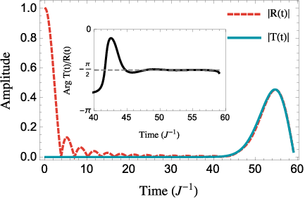
The dynamics of $R(t)$ and $T(t)$ in the 50/50 regime is shown in Fig. 2 when $L{=}51$. In Fig. 3 we report the results obtained for the $\beta^{50{/}50}$ values and for the factor $D$ as a function of the chain length $L$ for the uniform chain (red points). The damping factor is investigated via the output probability $P_{L}^{50/50}{=}|T(t^{*})|^{2}$ as a function of the chain length $L$, for a single particle in the initial state $|{\psi(0)}\rangle{=}a_{1}^{\dagger}|{0}\rangle$. We note that particle dispersion limits the observability of the beam splitter effects in long chains. In the following section we analyze how an extra minimal engineering of the couplings can improve the efficiency of our scheme.

The possibility to generate an effective beam splitter transformation between distant sites opens up to generate multi-particle interference effects. Peculiar quantum statistical effects appear when there are two traveling particles initially located at opposite boundary sites $1,L$. When $U{\to}\infty$ the Bose-Hubbard Hamiltonian (1) describes hard-core bosons and the system is equivalent, via the Jordan-Wigner transformation, to a spin-$\frac{1}{2}$ chain with XX interactions [33]. In our simulations, the dynamics of hard-core bosons and fermions are indistinguishable. The evolution is described in the Schrödinger picture by the state $|{\Psi(t)}\rangle{=}\sum_{jk}A_{jk}^{b/f}(t)a_{j}^{\dagger}a_{k}^{\dagger}|{0}\rangle$, where the subscript b/ f explicitly denotes the bosonic/fermionic case. Here $A_{jk}^{b}(t){=}A_{jk}(t){/}\sqrt{1+\delta_{jk}}$ for two bosons, while $A_{jk}^{f}(t){=}A_{jk}(t)$ for two fermions. The amplitudes $A_{jk}(t)$ evolve through the Schrödinger equation as $i\dot{A}_{jk}(t){=}\sum_{mn}K_{jk,mn}A_{mn}(t)$, where $A_{jk}(0){=}\delta_{j1}\delta_{kL}$ and $K_{jk,mn}$ is obtained from (1) via the algebra of commutation relations and $\hbar{\equiv}1$. We set $A_{jk}{=}0$ for $j{>}k$ ($j{\geq}k$) for bosons (fermions).

The two-particle interference effects are studied via the correlator $P_{jk}^{b/f}(t){=}\langle{\Psi(t)}|a_{j}^{\dagger}a_{k}^{\dagger}a_{k}a_{j}|{\Psi(t)}\rangle$ between two sites $j$,$k$ ($j{\leq}k$) [63] that in turn can be expressed in terms of probability amplitudes $A_{jk}(t)$ by using the Wick theorem. When $U{=}0$ the model is quasi-free and $P^{b/f}_{1L}(t){=}|T^{2}(t){\pm}R^{2}(t)|^{2}$, $P^{b}_{11}(t){=}P^{b}_{LL}(t){=}4|T(t)R(t)|^{2}$. This quantity is experimentally accessible in an optical lattice implementation [9, 10, 11]. In the specific, in Ref.[9] single particles are initialized in the lattice and pairs of atoms in the same site are separated, with a magnetic gradient, prior to the detection to avoid light-assisted collision processes.

Owing to the explicit expression of the effective beam splitter operator (2), one obtains perfect bunching (anti-bunching) with bosons (fermions) at time $t^{*}$ when $\beta{=}\beta^{50/50}$. In Fig. 5 we show the correlator $P_{ij}$ for two particle initially in $|{\psi(0)}\rangle{=}a_{1}^{\dagger}a^{\dagger}_{L}|{0}\rangle$ for a chain with $L{=}21$ at $t{=}18J^{-1}$ (before $t^{*}$ to avoid boundary effects) in the $50{/}50$ beam splitter configuration, namely with $\beta{=}0.94$. Although the effect is damped in a homogeneous chain because of the dispersive transmission (i.e. $|D|{\neq}1$), for bosons we clearly observe an increase of the probability to have two particles on the same side of the chain, while fermions show a maximum of $P_{jk}$ when the two particles are in opposite sides. In Fig. 6 (top) the bunching/antibunching behavior is evaluated by studying the correlation function $C_{jk}{=}P_{jk}{-}P_{j}P_{k}$, where $P_{j}{=}\sum_{k}P_{jk}$ takes into account the distinguishable motion of the atoms in the lattice, as in [10, 18]. As shown in Fig. 5 and in Fig. 6, bosons bunch while fermions and hard-core bosons anti-bunch.

One important question to address is whether any bunching effect is observable without the impurity $\beta{=}0$ in the Hamiltonian (1). Hanbury Brown-Twiss correlations have been observed in an optical lattice when the two particles are initially in neighboring sites [9]. On the other hand, when the particles are initially in distant sites no bunching effect appears even when the onsite interaction $U{/}J$ is not zero. This is shown in the lower panel of Fig. 6, where the correlation function $C_{jk}$ between two particles initially in sites $1$ and $L$ is plotted when $\beta{=}0$. A similar conclusion was given in Ref.[18] where two particles initially separated by an empty site were analyzed. These results justify the importance of introducing an optical impurity to generate an effective beam splitter transformation for incoming wavepackets, and then to produce interference phenomena such as the Hong-Ou-Mandel effect between distant sites.

A finite $U$ reduces the double occupancy probability for two bosons on the same site and one expects a transition from bunching to anti-bunching when $U$ goes from 0 to $\infty$. Our results show that $P_{jk}$ is almost indistinguishable from the fermion case when $U{\gtrsim}10J$. To highlight the transition from bosons to hard-core bosons in Fig. 7 we report the two particle correlator $P_{LL}(t^{*},\beta^{\rm opt})$ for different $U$ and $L{=}51$, in a uniform chain, normalized with respect to the $U{=}0$ case. For fixed $U$, $t^{*}$ and $\beta^{\rm opt}$ are found numerically by maximizing $P_{LL}(t,\beta)$ around $t{\sim}L/J$ and $\beta{\sim}1$. As shown in the inset of Fig. 7, the observed optimal $\beta$ for different $U$ is approximately equal to the value $\beta^{\rm 50/50}$ obtained when $U{=}0$. In fact, in the inset of Fig. 7 we plot the two-particle correlation $P_{LL}(t^{*})$ as a function of the impurity strength $\beta$, and we can clearly see that the $\beta$ which maximizes ${P}_{LL}$ is almost independent on $U$. For $U{\lesssim}0.1J$ the bunching effect is almost unaffected, while for $U{\gtrsim}3J$ a power law decay occurs and there is a rapid change of behavior near $U{\simeq}J$. The threshold value $U^{c}$ separating the two regions is obtained by fitting the data in the power law region and taking the intersection value with the unit constant line. For $L{=}51$ in particular we estimate $U^{c}{\simeq}0.71J$. The estimated $U^{c}$ is surprisingly similar to the critical value of the Mott insulator transition at the boundaries of a one dimensional chain (coordination number $z{=}1$) [64, 65]. This numerical evidence raises interesting questions on the possibility to detect the Mott phase transition via specific features of the chain’s non-equilibrium evolution.

It is worth mentioning that the weakly interacting regime $U{/}J{<}1$ is realized in [9], but also that the non-interacting regime $U{=}0$ has been experimentally achieved with Cs atoms loaded in a one-dimensional lattice, exploiting Feshbach resonances [66]. In view of other possible experimental applications with different atoms, we study in more detail how the bunching effect is affected by the interaction. We evaluate the relative variation of the two particle correlator $|\Delta P_{LL}|{/}P_{LL}(0)$, where $\Delta P_{LL}{\equiv}|P_{LL}(u){-}P_{LL}(0)|$, as a function of the on-site interaction $u{=}U{/}J$ for a uniform chain with different chain lengths $L$. As it is shown in Fig. 8 the relative variation is lower than 5% in the range $0.06{<}u{<}0.1$, and the threshold depends on the chain length. We argue that this effect is due to the larger spatial extent of the two traveling wavepackets ($\approx L^{1/3}$) that, accordingly, interact for more time in longer chains.

All the three optical elements which form a Mach-Zehnder interferometer can be obtained in a lattice: beam splitters have already been discussed; mirrors are implemented by boundary reflections and a phase shift can be obtained by freezing the hopping so that the system acquires a phase because of the chemical potential. Alternatively a phase shift can be obtained by applying a localized field in a site different from the middle one. However, this does not allow for a continuous control on the generated phase factor and has the further disadvantage that, in this case, the reflected and the transmitted components reach the two edges at different times.

In view of experimental applications, it is more compelling to devise a scheme which minimizes the dynamical control required on the chain. We show that the combined action of a beam splitter and a local phase-shifter can be achieved by applying a different optical potential to the right half of the chain: $\mu_{j}{=}J\gamma_{R}$ for $j{>}N{+}1$, being again $\mu_{N{+}1}{=}J\beta^{50/50}$, and $\mu_{j}{=}0$, $j{\leq}N$. When $\gamma_{R}{\neq}0$ a particle acquires a tunable phase $\phi{\propto}\gamma_{R}$ while it travels in the right part of the chain. We find that an effective 50/50 beam splitter can be obtained also when $\gamma_{R}{\neq}0$ by tuning $\beta^{50/50}_{\gamma_{R}}{\simeq}\beta_{\gamma_{R}{=}0}^{50/50}{\simeq}1$. As in the $\gamma_{R}{=}0$ case, the scattering matrix can be approximately factorized as $S_{\phi}(t^{*}){\simeq}D\tilde{S}_{\phi}(t^{*})$, being $D$ a damping factor and $\tilde{S}_{\phi}$ a unitary matrix. When $\beta{=}\beta^{50/50}_{\gamma_{R}}$ the latter is found to be $\tilde{S}_{\phi}{\simeq}\frac{1}{\sqrt{2}}\begin{pmatrix}1&-ie^{i\phi}\\ -ie^{i\phi}&e^{2i\phi}\end{pmatrix}~$ where $\phi{=}\gamma_{R}t^{*}/\pi$ namely $\tilde{S}_{\phi}$ is a composition of a 50/50 beam splitter and two phase shifts. By applying the unitary matrix $\tilde{S}_{\phi}$ twice one obtains an optical operation which is equivalent (up to local phase shifts) to a Mach-Zehnder unitary operation [67] (with phase $2\phi$).

As an interesting application, we show that by properly tuning the phase $\phi{\propto}\gamma_{R}$ one can vary the probability outcomes on the two output ports: as in a Mach-Zehnder interferometer [67], depending on $\phi$ a particle traveling from site 1 goes to site $1$ or $L$ after time $2t^{*}$.

This effect is shown in Fig. 9 for a $L{=}51$ chain where we used the double optimal engineering scheme [62] to minimize the dispersion and make $D{\simeq}1$.

We have proposed a strategy to simulate arbitrary linear optics networks with minimal control on static (potentially remote) bosons in a many-site lattice. Our scheme do not require an active atomic transport with external potential, while it exploits the natural atom dynamics (the quantum walk). Ultracold atoms in optical lattices are the most natural realization in view of recent unprecedented improvements in initialization and measurements [11, 10, 9, 45]. In particular, compared to purely photonic setups, opening up this alternative arena for linear optics can have the advantages of Fock-state (e.g. single atom) preparation (98% fidelity [9]), naturally a very large numbers of modes (sites), and potentially a higher detection efficiency (99% fidelity [50]) of a single atom in comparison to a single photon.

We have shown that fundamental operations between arbitrary remote sites are obtained by mixing quantum walks with suitably inserted local impurities. Several applications are considered; in particular, the achievement of a 50/50 remote beam splitter, a Mach-Zehnder interferometer, and the two-mode Hong-Ou-Mandel effect – rather robust against on-site interactions between atoms till a transition from bosonic to fermionic behavior close to the superfluid-Mott critical point. Possible sources of imperfections are discussed in the Appendix C. Since atoms can be prepared and detected with high efficiency, our scheme may pave the way for the study of interference effects in a many-boson optical lattice, such as the boson sampling. Moreover, our beam splitters, in conjunction with on-site interactions, should open up varied possibilities for generating non-classical states [68].

In relation to recent experiments showing the Hong-Ou-Mandel effect in adjacent wells [8], our protocol opens up to scalable generalizations to many-site lattices.

References

- [1] E. Knill, R. Laflamme, G. J. Milburn, Nature 409, 46 (2001).
- [2] S. Popescu, Phys. Rev. Lett 99, 130503 (2007).
- [3] S. Aaronson, A. Arkhipov, Theory of Computing, Volume 9(4), 143-252 (2013).
- [4] A. Crespi, et al., Nat. Photon. 7, 545 (2013).
- [5] J. B. Spring et al., Science 339, 798 (2013).
- [6] M. Tillmann, B. Dakic, R. Heilmann, S. Nolte, A. Szameit, and ´ P. Walther, Nat. Photonics 7, 540 (2013).
- [7] M. A. Broome, A. Fedrizzi, S. Rahimi-Keshari, J. Dove, S. Aaronson, T. C. Ralph, and A. G. White, Science 339, 794 (2013).
- [8] A. M. Kaufman, et al., Science 345, 306 (2014).
- [9] P.M. Preiss, et al., Science 347, 1229 (2015)
- [10] T. Fukuhara, et al., Nature 502, 76 (2013).
- [11] T. Fukuhara, et al., Nature Physics 9, 235 (2013).
- [12] S. Bose, Nature 502, 40 (2013) .
- [13] L. Sansoni, et al., Phys. Rev. Lett. 108, 010502 (2012).
- [14] A. Crespi, et al., Nature Photonics 7, 322 (2013).
- [15] W Liu, N. Andrei, Phys. Rev. Lett. 112, 257204 (2014).
- [16] G. M. Nikolopoulos, D. Petrosyan and P. Lambropoulos, J. Phys.: Condens. Matter 16, 4991 (2004)
- [17] X. Qin, Y. Ke, X. Guan, Z. Li, N. Andrei, C. Lee, arXiv: 1402.3349 (2014).
- [18] Y. Lahini, et al., Phys. Rev. A 86, 011603R (2012).
- [19] Y. Omar, N. Paunković, L. Sheridan, S. Bose. Phys. Rev. A 74, 042304 (2006).
- [20] C. K. Hong, Z. Y. Ou, L. Mandel, Phys. Rev. Lett 59, 2044 (1987).
- [21] R. J. Lewis-Swan, K. V. Kheruntsyan, Nat. Comm. 5 (2014).
- [22] M. Leder, C. Grossert, M. Weitz, Nat. Comm. 5, 3327 (2014).
- [23] T. Kovachy, J.M. Hogan, D.M.S. Johnson, M.A. Kasevich, Phys. Rev. A, 82, 013638 (2010).
- [24] L. Banchi, E. Compagno, S. Bose, Phys. Rev. A. 91, 052323 (2015).
- [25] D. Jaksch, H.-J. Briegel, J. I. Cirac, C. W. Gardiner, P. Zoller, Phys. Rev. Lett. 82, 1975 (1999).
- [26] O. Mandel, M. Greiner, A. Widera, T. Rom, T. W. Hänsch, I. Bloch, Nature 425, 937 (2003).
- [27] T. Wilk, et al., Phys. Rev. Lett. 104, 010502 (2010).
- [28] L. Isenhower, et al., Phys. Rev. Lett. 104, 010503 (2010).
- [29] T. Calarco, U. Dorner, P. S. Julienne, C. J. Williams, P. Zoller, Phys. Rev. A 70, 012306 (2004).
- [30] C. Weitenberg, S. Kuhr, K. Mølmer, J. F. Sherson, Phys. Rev. A 84, 032322 (2011).
- [31] M. Anderlini, P. J. Lee, B. L. Brown, J. Sebby-Strabley, W. D. Phillips, J. V. Porto, Nature 448, 452 (2007)
- [32] G. De Chiara, T. Calarco, M. Anderlini, S. Montangero, P. J. Lee, B. L. Brown, W. D. Phillips, and J. V. Porto Phys. Rev. A 77, 052333 (2008)
- [33] M. Lewenstein, A. Sanpera, V. Ahufinger, Ultracold Atoms in Optical Lattices, (Oxford University Press, Oxford, 2012).
- [34] T. D. Kühner, H. Monien, Phys. Rev. B 58, R14741(R) (1998).
- [35] S. Rapsch, U. Schollwöck and W. Zwerger, Europhys. Lett. 46, 559 (1999).
- [36] D. Jaksch, C. Bruder, J. I. Cirac, C. W. Gardiner, P. Zoller, Phys. Rev. Lett 81, 3108 (1998)
- [37] M. Greiner, O. Mandel, T. Esslinger, T. W. Hänsch, I. Bloch, Nature 415, 39 (2002).
- [38] M. Rigol, A. Muramatsu, Phys. Rev. A 70,031603 (2004).
- [39] R. Jördens, N. Strohmaier, K. Günter, H. Moritz, T. Esslinger, Nature 455 204 (2008).
- [40] G. Modugno, F. Ferlaino, R. Heidemann, G. Roati, M. Inguscio, Phys. Rev A. 68,011601 (2003).
- [41] M. J. Hartmann, F. GSL Brandao, Fernando M. B. Plenio, Nature 2,849 (2006).
- [42] G. M. Nikolopoulos, D. Petrosyan, P. Lambropoulos, Journal of Physics: Condensed Matter 16, 4991 (2004).
- [43] M. Bellec, G. M. Nikolopoulos, S. Tzortzakis, Optics Letters 37, 4504 (2012).
- [44] Z.-M. Wang, L.-A. Wu, M. Modugno, W. Yao, B. Shao, Sci. Rep. 3, (2013).
- [45] W. S. Bakr, J. I. Gillen, A. Peng, S. Fölling, M. Greiner, Nature 462, 74 (2009).
- [46] H. Pichler, A. J. Daley, P. Zoller, Phys. Rev. A. 82, 063605 (2010).
- [47] S. Sarkar, S. Langer, J. Schachenmayer, and A. J. Daley, Phys. Rev. A 90, 023618 (2014).
- [48] C. Weitenberg, et al., Nature 471, 319324 (2011).
- [49] P. Würtz, T. Langen, T. Gericke, A. Koglbauer, H. Ott, Phys. Rev. Lett. 103, 080404 (2009).
- [50] C. Gross, I. Bloch, arXiv:1409.8501 (2014)
- [51] M. Schreiber, S. S. Hodgman, P. Bordia, H. P. Lüschen, M. H. Fischer, R. Vosk, Ronen, E. Altman, U. Schneider, I. Bloch, arXiv:1501.05661 (2015).
- [52] P. M. Preiss, R. Ma, M. E. Tai, J. Simon, M. Greiner, Phys. Rev. A 91, 041602 (2015)
- [53] M. Reck, A. Zeilinger, H. J. Bernstein, P. Bertani, Phys. Rev. Lett 73, 58 (1994).
- [54] L. Banchi, R. Vaia, J. Math. Phys. 54, 043501 (2013).
- [55] A. Bayat, L. Banchi, S. Bose, P. Verrucchi, Phys. Rev. A 83, 062328 (2011).
- [56] G. M. Nikolopoulos, I. Jex, Quantum state transfer and network engineering, Springer, New York, 2014 .
- [57] A. Kay, Int. J. Quantum Inform., 08, 641 (2010)
- [58] M. Christandl, N. Datta, A. Ekert, and A. J. Landahl, Phys. Rev. Lett. 92, 187902 (2004).
- [59] S. R. Clark, C. Moura Alves, and D. Jaksch, New Journal of Physics 7, 124 (2005).
- [60] R. Sousa, Y. Omar, New J. Phys. 16, 123003 (2014)
- [61] L. Banchi, T. J. G. Apollaro, A. Cuccoli, R. Vaia, P. Verrucchi, New. J. Phys. 13, 123006 (2011)
- [62] T. J. G. Apollaro, L. Banchi, A. Cuccoli, R. Vaia, P. Verrucchi, Phys. Rev. A. 85, 052319 (2012)
- [63] Y. Bromberg, Y. Lahini, R. Morandotti, Y. Silberberg, Phys. Rev. Lett 102, 253904 (2009).
- [64] I. Danshita and A. Polkovnikov, Phys. Rev. A 84, 063637 (2011).
- [65] M. Greiner, Ph.D. thesis, Ludwig-Maximilians-Universität München, 2003.
- [66] F. Meinert, et. al., Phys. Rev. Lett. 112, 193003 (2014).
- [67] S. Haroche, J. M. Raimond, Exploring the Quantum: Atoms, Cavities, and Photons, (Oxford University Press, New York, 2013).
- [68] T. Fogarty, A. Kiely, S. Campbell, T. Busch, Phys. Rev. A 87, 043630 (2013).
- [69] M. Abramowitz and I. A. Stegun, Handbook of Mathematical Functions, (Dover Publications Inc., New York, 1965).