跳到论文正文
W Papers独立论文阅读器 arXiv:1407.8483 论文正文 计算阅读时间 · 0%
引用这篇论文根据当前论文元数据生成,正式投稿前建议核对。


License: arXiv.org perpetual non-exclusive license
arXiv:1407.8483v2 [math-ph] 20 Feb 2015

Six-vertex model with partial domain wall boundary conditions: ferroelectric phaseThanks: The first author is supported in part by the National Science Foundation (NSF) Grant DMS-1265172.

Pavel Bleher Address: Department of Mathematical Sciences, Indiana University-Purdue University Indianapolis, 402 N. Blackford St., Indianapolis, IN 46202, U.S.A. Email address: bleher@math.iupui.edu and Karl Liechty Address: Department of Mathematical Sciences, DePaul University, Chicago, IL 60614, U.S.A. Email address: kliechty@depaul.edu
Date: August 24, 2026
Abstract.

We obtain an asymptotic formula for the partition function of the six-vertex model with partial domain wall boundary conditions in the ferroelectric phase region. The proof is based on a formula for the partition function involving the determinant of a matrix of mixed Vandermonde/Hankel type. This determinant can be expressed in terms of a system of discrete orthogonal polynomials, which can then be evaluated asymptotically by comparison with the Meixner polynomials.

1. Introduction

We consider the the six-vertex model on a rectangular lattice of size (n−m)×n(n-m)\times n for any positive integer nn and any integer mm with 0≤m<n0\leq m<n. The states of the model are realized by placing arrows on edges of the lattice obeying the ice rule, meaning that at each vertex there are exactly two arrows pointing in and two arrows pointing out. There are six possible configurations of arrows at each vertex, and we label the six vertex types as shown in Fig. 1. The partial domain wall boundary conditions (pDWBC) are defined in the following way. On the left and right boundaries all arrows point out of the lattice, and on the bottom boundary all arrows point in. The top boundary is free, and the ice-rule implies that there are exactly mm arrows pointing out on this boundary, and the remaining (n−m)(n-m) arrows point in. In Fig. 2 below, an example of the arrow configuration with the partial domain wall boundary conditions is shown on the 3×53\times 5 lattice.

For each of the six vertex types we assign a weight wiw_{i}, i=1,…,6i=1,\dots,6, and define the weight of an arrow configuration as the product of the weights of the vertices in the configuration. That is, for a configuration σ\sigma of arrows, its weight w⁡(σ)w(\sigma) is defined to be

w⁡(σ)=∏x∈Vn−m,nwt⁡(x,σ)=∏j=16wiNi​(σ),w(\sigma)=\prod_{x\in V_{n-m,n}}w_{t(x;\sigma)}=\prod_{j=1}^{6}w_{i}^{N_{i}(\sigma)}\,, (1.1)

where Vn−m,nV_{n-m,n} is the set of vertices in the lattice, t⁡(x,σ)t(x;\sigma) is the type of vertex at the vertex x∈Vn−m,nx\in V_{n-m,n} in the configuration σ\sigma, and Ni​(σ)N_{i}(\sigma) is the number of vertices of type ii in the configuration σ\sigma. The Gibbs measure on states is then defined as

μ⁡(σ)=w⁡(σ)Zn−m,n,Zn−m,n≡Zn−m,n​(w1,w2,w3,w4,w5,w6)=∑σw⁡(σ),\mu(\sigma)=\frac{w(\sigma)}{Z_{n-m,n}}\,,\qquad Z_{n-m,n}\equiv Z_{n-m,n}(w_{1},w_{2},w_{3},w_{4},w_{5},w_{6})=\sum_{\sigma}w(\sigma), (1.2)

where Zn−m,nZ_{n-m,n} is the partition function, and the sum is over all configurations obeying the pDWBC.

Refer to caption
Figure 1. The six types of vertices allowed under the ice-rule.
Refer to caption
Figure 2. An example of the arrow configuration with the partial domain wall boundary conditions on the 3×53\times 5 lattice.

When m=0m=0, the pDWBC reduces to the domain wall boundary conditions on the n×nn\times n lattice [10], and the asymptotic expansion of the partition function Zn,nZ_{n,n} as n→∞n\to\infty has been studied in detail in a series of papers by the first author of the current paper and various coauthors. For a complete description, see the monograph [3] of the current authors. The main purpose of the current work is to obtain an asymptotic expansion for the pDWBC partition function as well. Let us also note that the pDWBC partition function has recently appeared in the literature as an expression for certain quantities related to the XXX spin chain, and related models in mathematical physics, see [11], [5], and references therein.

1.1. Conservation laws and reduction of parameters

A priori the six-vertex model has six parameters: the weights w1,…,w6w_{1},\dots,w_{6}. By observing some quantities which are conserved in each state, we can reduce the number of parameters to three. Namely we have the following proposition.

Proposition 1.1.

In the six-vertex model on the (n−m)×n(n-m)\times n lattice, the following equations hold for every state σ\sigma satisfying pDWBC:

N1​(σ)+N2​(σ)+N3​(σ)+N4​(σ)+N5​(σ)+N6​(σ)\displaystyle N_{1}(\sigma)+N_{2}(\sigma)+N_{3}(\sigma)+N_{4}(\sigma)+N_{5}(\sigma)+N_{6}(\sigma) =n⁡(n−m),\displaystyle=n(n-m), (1.3)
N5​(σ)−N6​(σ)\displaystyle N_{5}(\sigma)-N_{6}(\sigma) =n−m,\displaystyle=n-m,
N1​(σ)−N2​(σ)+N4​(σ)−N3​(σ)\displaystyle N_{1}(\sigma)-N_{2}(\sigma)+N_{4}(\sigma)-N_{3}(\sigma) =m⁡(n−m).\displaystyle=m(n-m).

The first equation in (1.3) is trivial and simply counts the total number of vertices. The second equation follows from the fact that in each row there is one more type-5 vertex than type-6 vertex, which is a direct consequence of the domain wall boundary condition in each row. We prove the third equation in Appendix A in the end of the paper.

Remark: In the case m=0m=0, the third equation of (1.3) can be split into the two equations N1​(σ)−N2​(σ)=N4​(σ)−N3​(σ)=0N_{1}(\sigma)-N_{2}(\sigma)=N_{4}(\sigma)-N_{3}(\sigma)=0, giving four conserved quantities. In this case the general six-vertex model can be reduced to two parameters, see [2], [3].

Let us now discuss how to use Proposition 1.1 to reduce the number of parameters. Let us write

w1=a​e−α,w2=a​eα,w3=b​e−β,w4=b​eβ,w5=c​e−ξ,w6=c​eξ,w_{1}=ae^{-\alpha},\quad w_{2}=ae^{\alpha},\quad w_{3}=be^{-\beta},\quad w_{4}=be^{\beta},\quad w_{5}=ce^{-\xi},\quad w_{6}=ce^{\xi}, (1.4)

where

a=w1​w2,eα=w2w1,b=w3​w4,eβ=w4w3,\displaystyle a=\sqrt{w_{1}w_{2}},\quad e^{\alpha}=\sqrt{\frac{w_{2}}{w_{1}}}\,,\quad b=\sqrt{w_{3}w_{4}},\quad e^{\beta}=\sqrt{\frac{w_{4}}{w_{3}}}\,, (1.5)
c=w5​w6,eξ=w6w5.\displaystyle c=\sqrt{w_{5}w_{6}},\quad e^{\xi}=\sqrt{\frac{w_{6}}{w_{5}}}\,.

Then

w1N1​w2N2​w3N3​w4N4​w5N5​w6N6=aN1+N2​bN3+N4​cN5+N6​eα⁡(N2−N1)+β⁡(N4−N3)+ξ⁡(N6−N5)w_{1}^{N_{1}}w_{2}^{N_{2}}w_{3}^{N_{3}}w_{4}^{N_{4}}w_{5}^{N_{5}}w_{6}^{N_{6}}=a^{N_{1}+N_{2}}b^{N_{3}+N_{4}}c^{N_{5}+N_{6}}e^{\alpha(N_{2}-N_{1})+\beta(N_{4}-N_{3})+\xi(N_{6}-N_{5})} (1.6)

Let

α=η+θ,β=η−θ;η=α+β2,θ=α−β2.\alpha=\eta+\theta,\quad\beta=\eta-\theta;\qquad\eta=\frac{\alpha+\beta}{2}\,,\quad\theta=\frac{\alpha-\beta}{2}\,. (1.7)

Then

w1N1​w2N2​w3N3​w4N4​w5N5​w6N6\displaystyle w_{1}^{N_{1}}w_{2}^{N_{2}}w_{3}^{N_{3}}w_{4}^{N_{4}}w_{5}^{N_{5}}w_{6}^{N_{6}} =aN1+N2​bN3+N4​cN5+N6\displaystyle=a^{N_{1}+N_{2}}b^{N_{3}+N_{4}}c^{N_{5}+N_{6}} (1.8)
×eη⁡(N2−N1+N4−N3)+θ⁡(N2−N1−N4+N3)+ξ⁡(N6−N5)\displaystyle\times e^{\eta(N_{2}-N_{1}+N_{4}-N_{3})+\theta(N_{2}-N_{1}-N_{4}+N_{3})+\xi(N_{6}-N_{5})}

Using the second and third equations of (1.3), we obtain that

w1N1​w2N2​w3N3​w4N4​w5N5​w6N6\displaystyle w_{1}^{N_{1}}w_{2}^{N_{2}}w_{3}^{N_{3}}w_{4}^{N_{4}}w_{5}^{N_{5}}w_{6}^{N_{6}} =aN1+N2​bN3+N4​cN5+N6​eη⁡(N2−N1+N4−N3)−θ​m​(n−m)−ξ⁡(n−m)\displaystyle=a^{N_{1}+N_{2}}b^{N_{3}+N_{4}}c^{N_{5}+N_{6}}e^{\eta(N_{2}-N_{1}+N_{4}-N_{3})-\theta m(n-m)-\xi(n-m)} (1.9)
=(a​e−η)N1​(a​eη)N2​(b​e−η)N3​(b​eη)N4​cN5​cN6​e−θ​m​(n−m)−ξ⁡(n−m).\displaystyle=(ae^{-\eta})^{N_{1}}(ae^{\eta})^{N_{2}}(be^{-\eta})^{N_{3}}(be^{\eta})^{N_{4}}c^{N_{5}}c^{N_{6}}e^{-\theta m(n-m)-\xi(n-m)}.

From (1.5), (1.7),

e−θ=(w1​w4w2​w3)1/4,e−ξ=(w5w6)1/2,e^{-\theta}=\left(\frac{w_{1}w_{4}}{w_{2}w_{3}}\right)^{1/4},\quad e^{-\xi}=\left(\frac{w_{5}}{w_{6}}\right)^{1/2}, (1.10)

hence

w1N1​w2N2​w3N3​w4N4​w5N5​w6N6\displaystyle w_{1}^{N_{1}}w_{2}^{N_{2}}w_{3}^{N_{3}}w_{4}^{N_{4}}w_{5}^{N_{5}}w_{6}^{N_{6}} =(a​e−η)N1​(a​eη)N2​(b​e−η)N3​(b​eη)N4​cN5​cN6\displaystyle=(ae^{-\eta})^{N_{1}}(ae^{\eta})^{N_{2}}(be^{-\eta})^{N_{3}}(be^{\eta})^{N_{4}}c^{N_{5}}c^{N_{6}} (1.11)
×(w1​w4w2​w3)m⁡(n−m)/4​(w5w6)(n−m)/2.\displaystyle\times\left(\frac{w_{1}w_{4}}{w_{2}w_{3}}\right)^{m(n-m)/4}\left(\frac{w_{5}}{w_{6}}\right)^{(n-m)/2}.

This implies the relation between partition functions,

Zn−m,n​(w1,w2,w3,w4,w5,w6)\displaystyle Z_{n-m,n}(w_{1},w_{2},w_{3},w_{4},w_{5},w_{6}) =(w1​w4w2​w3)m⁡(n−m)/4​(w5w6)(n−m)/2\displaystyle=\left(\frac{w_{1}w_{4}}{w_{2}w_{3}}\right)^{m(n-m)/4}\left(\frac{w_{5}}{w_{6}}\right)^{(n-m)/2} (1.12)
×Zn−m,n​(a​e−η,a​eη,b​e−η,b​eη,c,c),\displaystyle\times Z_{n-m,n}(ae^{-\eta},ae^{\eta},be^{-\eta},be^{\eta},c,c),

and between Gibbs measures,

μ⁡(σ,w1,w2,w3,w4,w5,w6)=μ⁡(σ,a​e−η,a​eη,b​e−η,b​eη,c,c).\mu(\sigma;w_{1},w_{2},w_{3},w_{4},w_{5},w_{6})=\mu(\sigma;ae^{-\eta},ae^{\eta},be^{-\eta},be^{\eta},c,c). (1.13)

Furthermore, using the first equation of (1.3), we have

Zn−m,n​(a​e−η,a​eη,b​e−η,b​eη,c,c)\displaystyle Z_{n-m,n}(ae^{-\eta},ae^{\eta},be^{-\eta},be^{\eta},c,c) =cn⁡(n−m)​Zn−m,n​(a​e−ηc,a​eηc,b​e−ηc,b​eηc,1,1),\displaystyle=c^{n(n-m)}Z_{n-m,n}\left(\frac{ae^{-\eta}}{c},\frac{ae^{\eta}}{c},\frac{be^{-\eta}}{c},\frac{be^{\eta}}{c},1,1\right), (1.14)
μ⁡(σ,a​e−η,a​eη,b​e−η,b​eη,c,c)\displaystyle\mu(\sigma;ae^{-\eta},ae^{\eta},be^{-\eta},be^{\eta},c,c) =μ⁡(σ,a​e−ηc,a​eηc,b​e−ηc,b​eηc,1,1),\displaystyle=\mu\left(\sigma;\frac{ae^{-\eta}}{c},\frac{ae^{\eta}}{c},\frac{be^{-\eta}}{c},\frac{be^{\eta}}{c},1,1\right),

and so the model reduces to the three parameters, ac,bc,\frac{a}{c}\,,\;\frac{b}{c}\,, and η\eta.

1.2. The main result: asymptotics of the partition function

Fix two real parameters tt and γ\gamma, with 0<|γ|<t0<|\gamma|<t, and introduce the parameterization of aa, bb, cc as

a=sinh(t−γ),b=sinh(t+γ),c=sinh(2|γ|).\displaystyle a=\sinh(t-\gamma)\,,\quad b=\sinh(t+\gamma)\,,\quad c=\sinh(2|\gamma|). (1.15)

Set

a±=e±γa,b±=e±γb.\displaystyle a_{\pm}=e^{\pm\gamma}a\,,\qquad b_{\pm}=e^{\pm\gamma}b\,. (1.16)

In the current work we consider the partition function

Zn−m,n​(a−,a+,b−,b+,c,c)=Zn−m,n​(a​e−γ,a​eγ,b​e−γ,b​eγ,c,c),Z_{n-m,n}(a_{-},a_{+},b_{-},b_{+},c,c)=Z_{n-m,n}(ae^{-\gamma},ae^{\gamma},be^{-\gamma},be^{\gamma},c,c), (1.17)

depending on the two parameters, tt and γ\gamma. It is a specialization of the three parameter family, Zn−m,n​(a​e−η,a​eη,b​e−η,b​eη,c,c)Z_{n-m,n}(ae^{-\eta},ae^{\eta},be^{-\eta},be^{\eta},c,c) in (1.12) to the case when η=γ\eta=\gamma.

Notice that 0<γ<t0<\gamma<t corresponds to the regime

b−​b+>a−​a++c2,b_{-}b_{+}>a_{-}a_{+}+c^{2}\,, (1.18)

and γ<0<|γ|<t\gamma<0<|\gamma|<t, corresponds to the regime

a−​a+>b−​b++c2.a_{-}a_{+}>b_{-}b_{+}+c^{2}\,. (1.19)

These two regimes are natural extensions of the two components of the ferroelectric regime considered in [2]. Without loss of generality we will consider only the component (1.18) corresponding to 0<γ<t0<\gamma<t.

Remark: According to the conservation laws (1.3),

Zn−m,n​(a−,a+,b−,b+,c,c)\displaystyle Z_{n-m,n}(a_{-},a_{+},b_{-},b_{+},c,c) =e−γ⁡(m⁡(n−m)CLOSE​Zn−m,n​(a,a,e−2​γ​b,e2​γ​b,c,c)\displaystyle=e^{-\gamma(m(n-m)}Z_{n-m,n}(a,a,e^{-2\gamma}b,e^{2\gamma}b,c,c) (1.20)
=e−m⁡(n−m)​γ​an⁡(n−m)​Zn−m,n​(1,1,e−2​γ​ba,e2​γ​ba,ca,ca),\displaystyle=e^{-m(n-m)\gamma}a^{n(n-m)}Z_{n-m,n}\left(1,1,\frac{e^{-2\gamma}b}{a},\frac{e^{2\gamma}b}{a},\frac{c}{a},\frac{c}{a}\right),

where the weights in the latter equation match the weights which appear in [5] after a simple change of variables.

Our main results concern the asymptotic behavior of the partition function Zn−m,nZ_{n-m,n} as n→∞n\to\infty.

Theorem 1.2.

Fix two parameters t,γt,\gamma with 0<t<γ0<t<\gamma, and let

Zn−m,n≡Zn−m,n​(a−,a+,b−,b+,c,c),Z_{n-m,n}\equiv Z_{n-m,n}(a_{-},a_{+},b_{-},b_{+},c,c), (1.21)

where a±,b±,a_{\pm},b_{\pm}, and cc are as in (1.15), (1.16). Fix any ε>0\varepsilon>0. Then there is a constant κ>0\kappa>0 such that as n→∞n\to\infty,

Zn−m,n=[sinh⁡(t+γ)]n⁡(n−m)​em⁡(n−m)​γ​e−(n−m)​(t−γ)​[1+𝒪⁡(e−κ​n)],Z_{n-m,n}=[\sinh(t+\gamma)]^{n(n-m)}e^{m(n-m)\gamma}\,e^{-(n-m)(t-\gamma)}\big[1+\mathcal{O}(e^{-\kappa n})\big], (1.22)

uniformly with respect to mm in the interval

n​ε≤m<n.n\varepsilon\leq m<n. (1.23)

Remark. Observe that there is no constant factor in (1.22), i.e., the constant factor is 1. In addition, the error term is exponentially small. This should be compared with the paper [2] (see also [3]), where a similar result was obtained for m=0m=0.

The case of m≤n​εm\leq n\varepsilon, including when mm remains bounded, is covered by the following theorem.

Theorem 1.3.

Fix the parameters of the six-vertex models as in Theorem 1.2. For any ε>0\varepsilon>0 there is a constant n0>0n_{0}>0 such that for any n≥n0n\geq n_{0} and any 0≤m<n0\leq m<n,

Zn−m,n=C⁡(m)​[sinh⁡(t+γ)]n⁡(n−m)​em⁡(n−m)​γ​e−(n−m)​(t−γ)​(1+ξn​m),Z_{n-m,n}=C(m)[\sinh(t+\gamma)]^{n(n-m)}e^{m(n-m)\gamma}\,e^{-(n-m)(t-\gamma)}\big(1+\xi_{nm}\big), (1.24)

where

C⁡(m)=1−e−4​γ​(m+1),C(m)=1-e^{-4\gamma(m+1)}, (1.25)

and

|ξn​m|≤ρm​e−n1−ε,ρ=e−2​γ<1.|\xi_{nm}|\leq\rho^{m}e^{-n^{1-\varepsilon}},\quad\rho=e^{-2\gamma}<1. (1.26)

The proofs of Theorems 1.2 and 1.3 are based on a determinantal formula for Zn−m,nZ_{n-m,n} and estimates for corresponding orthogonal polynomials. In fact, Theorem 1.2 follows from Theorem 1.3, but the proof of Theorem 1.3 is more involved, and to facilitate the reading we will first prove Theorem 1.2.

It is interesting to notice that the limiting free energy per site FF depends on the aspect ratio r=n−mnr=\frac{n-m}{n} of the rectangular lattice of size (n−m)×n(n-m)\times n. Namely, from (1.24),

F=limn,m→∞;n−mn→r1(n−m)​n​ln⁡Zn−m,n=ln⁡[sinh⁡(t+γ)]+(1−r)​γ.F=\lim_{n,m\to\infty;\;\frac{n-m}{n}\to r}\frac{1}{(n-m)n}\ln Z_{n-m,n}=\ln[\sinh(t+\gamma)]+(1-r)\gamma. (1.27)

Indeed, FF is determined entirely by the weight of the ground state configuration. Before proceeding with the proof of Theorems 1.2 and 1.3, let us briefly discuss the ground state.

1.3. Ground state configuration

The ground state configuration is the one with the largest weight. For the weights described in Theorem 1.2, the weight of a configuration σ\sigma is

w⁡(σ)\displaystyle w(\sigma) =(a−)N1​(σ)​(a+)N2​(σ)​(b−)N3​(σ)​(b+)N4​(σ)​(c)N5​(σ)+N6​(σ)\displaystyle=\left(a_{-}\right)^{N_{1}(\sigma)}\left(a_{+}\right)^{N_{2}(\sigma)}\left(b_{-}\right)^{N_{3}(\sigma)}\left(b_{+}\right)^{N_{4}(\sigma)}\left(c\right)^{N_{5}(\sigma)+N_{6}(\sigma)} (1.28)
=e−γ⁡(N1​(σ)−N2​(σ))​e−γ⁡(N3​(σ)−N4​(σ))​aN1​(σ)+N2​(σ)​bN3​(σ)+N4​(σ)​cN5​(σ)+N6​(σ).\displaystyle=e^{-\gamma(N_{1}(\sigma)-N_{2}(\sigma))}e^{-\gamma(N_{3}(\sigma)-N_{4}(\sigma))}a^{N_{1}(\sigma)+N_{2}(\sigma)}b^{N_{3}(\sigma)+N_{4}(\sigma)}c^{N_{5}(\sigma)+N_{6}(\sigma)}.

Using the conservation laws (1.3), we can write (1.28) as

w⁡(σ)\displaystyle w(\sigma) =e−m⁡(n−m)​γ​e2​γ​(N4​(σ)−N3​(σ))​aN1​(σ)+N2​(σ)​bN3​(σ)+N4​(σ)​cN5​(σ)+N6​(σ).\displaystyle=e^{-m(n-m)\gamma}e^{2\gamma(N_{4}(\sigma)-N_{3}(\sigma))}a^{N_{1}(\sigma)+N_{2}(\sigma)}b^{N_{3}(\sigma)+N_{4}(\sigma)}c^{N_{5}(\sigma)+N_{6}(\sigma)}. (1.29)

Since b>a+cb>a+c, we see that the ground state configuration is the one which maximizes both N4+N3N_{4}+N_{3} and N4−N3N_{4}-N_{3}. This is achieved by placing type-5 vertices along the up-left diagonal starting from the bottom-right corner. Above this diagonal all arrows point down or right, and so all vertices are of type 3. Below and to the left of this diagonal, all arrows point up or left, and so all vertices are of type 4. See Fig. 3 for the ground state configuration on the 4×74\times 7 lattice. The diagonal of type-5 vertices is circled.

Refer to caption
Figure 3. The ground state configuration on the 4×74\times 7 lattice. On the circled diagonal all vertices are of type 5. To the right of this diagonal all vertices are of type 3, and to the left of it all vertices are of type 4.

The weight of the ground state configuration σgs\sigma^{\textrm{gs}} is

w⁡(σgs)\displaystyle w(\sigma^{\textrm{gs}}) =(b+)(n−m)​(n+m−1)/2​(b−)(n−m)​(n−m−1)/2​cn−m\displaystyle=\left(b_{+}\right)^{(n-m)(n+m-1)/2}\left(b_{-}\right)^{(n-m)(n-m-1)/2}c^{n-m} (1.30)
=em⁡(n−m)​γ​b(n−m)​(n−1)​cn−m\displaystyle=e^{m(n-m)\gamma}b^{(n-m)(n-1)}c^{n-m}
=bn⁡(n−m)​em⁡(n−m)​γ​(cb)n−m.\displaystyle=b^{n(n-m)}e^{m(n-m)\gamma}\left(\frac{c}{b}\right)^{n-m}\,.

Comparing (1.22) and (1.24) with (1.30) we find that as m,n→∞m,n\to\infty,

Zn−m,nw⁡(σgs)=(e2​γ−e−2​te2​γ−e−2​γ)n−m​(1+ξn​m),\frac{Z_{n-m,n}}{w(\sigma^{\textrm{gs}})}=\left(\frac{e^{2\gamma}-e^{-2t}}{e^{2\gamma}-e^{-2\gamma}}\right)^{n-m}(1+\xi_{nm}), (1.31)

where ξn​m\xi_{nm} is estimated in Theorem 1.3. A comparison of (1.22) or (1.24) with (1.30) shows that the limiting free energy per site FF defined in (1.27) comes entirely from the ground state configuration. This was known for m=0m=0, see [2].

1.4. Outline of the rest of the paper

The rest of the paper is organized as follows. In section 2 we state the determinantal formula for the partition function Zn−m,nZ_{n-m,n}, and use it to write a formula for Zn−m,nZ_{n-m,n} in terms of certain orthogonal polynomials on the positive integer lattice. In section 3 we recall the Meixner polynomials, and in section 4 we introduce the Interpolation Problem in order to compare our orthogonal polynomials with the Meixner ones. In sections 5 and 6, we prove Theorem 1.2 by a careful comparison of the normalizing constants for our orthogonal polynomials with those of the Meixner polynomials. In section 7 the analogous analysis is carried out for the proof of Theorem 1.3, and in sections 8 and 9 the proof of Theorem 1.3 is completed by finding an explicit formula for the constant term C⁡(m)C(m) using the Toda equation. Finally, section 10 gives a short discussion of the phase transition in the underlying orthogonal polynomials.

2. An orthogonal polynomial formula for Zn−m,nZ_{n-m,n}

Introduce the notations

φ⁡(t):\displaystyle\varphi(t): =sinh⁡(t−γ)​sinh⁡(t+γ)=a​b,\displaystyle=\sinh(t-\gamma)\sinh(t+\gamma)=ab\,, (2.1)
ϕ⁡(t):\displaystyle\phi(t): =sinh⁡(2​γ)sinh⁡(t−γ)​sinh⁡(t+γ)=ca​b.\displaystyle=\frac{\sinh(2\gamma)}{\sinh(t-\gamma)\sinh(t+\gamma)}=\frac{c}{ab}\,.

The starting point for our analysis is the following determinantal formula for the partition function.

Proposition 2.1.

For the six-vertex model on the (n−m)×n(n-m)\times n lattice with pDWBC and weights as described in (1.15) – (1.16), the partition function Zn−m,nZ_{n-m,n} is given by the following formula:

Zn−m,n=(−1)m⁡(m+1)/2−n​m​φ​(t)n⁡(n−m)​em⁡(n−m)​t2m⁡(m−1)/2​∏j=0n−m−1j!​∏j=0n−1j!​τn−m,n,Z_{n-m,n}=\frac{(-1)^{m(m+1)/2-nm}\varphi(t)^{n(n-m)}e^{m(n-m)t}}{2^{m(m-1)/2}\prod_{j=0}^{n-m-1}j!\prod_{j=0}^{n-1}j!}\;\tau_{n-m,n},\\ (2.2)

where

τn−m,n:=det(1(−2)(−2)2…(−2)n−1⋱1(−2​m)(−2​m)2…(−2​m)n−1ϕ⁡(t)ϕ′​(t)ϕ′′​(t)…ϕ(n−1)​(t)ϕ′​(t)ϕ′′​(t)ϕ′′′​(t)…ϕ(n)​(t)⋱ϕ(n−m−1)​(t)ϕ(n−m)​(t)ϕ(n−m+1)​(t)…ϕ(2​n−m−2)​(t)),\tau_{n-m,n}:=\det\begin{pmatrix}1&(-2)&(-2)^{2}&\dots&(-2)^{n-1}\\ \vdots&\vdots&\vdots&\ddots&\vdots\\ 1&(-2m)&(-2m)^{2}&\dots&(-2m)^{n-1}\\ \phi(t)&\phi^{\prime}(t)&\phi^{\prime\prime}(t)&\dots&\phi^{(n-1)}(t)\\ \phi^{\prime}(t)&\phi^{\prime\prime}(t)&\phi^{\prime\prime\prime}(t)&\dots&\phi^{(n)}(t)\\ \vdots&\vdots&\vdots&\ddots&\vdots\\ \phi^{(n-m-1)}(t)&\phi^{(n-m)}(t)&\phi^{(n-m+1)}(t)&\dots&\phi^{(2n-m-2)}(t)\end{pmatrix}, (2.3)

is a determinant of mixed Vandermonde/Hankel type.

This proposition follows from the Izergin–Korepin formula for the partition function of the inhomogeneous six-vertex model with domain wall boundary conditions on the square lattice [6], [7]. A similar formula for the inhomogeneous six-vertex model was derived in [5]. For completeness, we present a proof in Appendix B. When m=0m=0, it simplifies to the usual formula for the partition function of the six-vertex model with domain wall boundary conditions:

Zn,n=[φ⁡(t)]n2∏j=0n−1(j!)2​τn,n,τn,n=det(ϕj+k−2​(t))j,k=1n.Z_{n,n}=\frac{[\varphi(t)]^{n^{2}}}{\prod_{j=0}^{n-1}(j!)^{2}}\;\tau_{n,n},\qquad\tau_{n,n}=\det\big(\phi^{j+k-2}(t)\big)_{j,k=1}^{n}. (2.4)

Remark: The proof of Proposition 2.1 relies on the particular parametrization (1.15) – (1.16) of the weights. For the general class of weights (1.12), there doesn’t seem to be any determinantal formula for the partition function unless η=γ\eta=\gamma. See the remark following the proof of lemma B.1

It is straightforward that for 0<γ<t0<\gamma<t, the function ϕ⁡(t)\phi(t) can be represented as the discrete Laplace transform

ϕ⁡(t)=2​∑x=1∞u⁡(x),u⁡(x):=2​e−2​t​x​sinh⁡(2​γ​x)=e−2​(t−γ)​x−e−2​(t+γ)​x.\phi(t)=2\sum_{x=1}^{\infty}u(x)\,,\qquad u(x):=2e^{-2tx}\sinh(2\gamma x)=e^{-2(t-\gamma)x}-e^{-2(t+\gamma)x}\,. (2.5)

Indeed,

2​∑x=1∞u⁡(x)\displaystyle 2\sum_{x=1}^{\infty}u(x) =2​∑x=1∞(e−2​(t−γ)​x−e−2​(t+γ)​x)=2​[e−2​(t−γ)1−e−2​(t−γ)−e−2​(t+γ)1−e−2​(t+γ)]\displaystyle=2\sum_{x=1}^{\infty}\left(e^{-2(t-\gamma)x}-e^{-2(t+\gamma)x}\right)=2\left[\frac{e^{-2(t-\gamma)}}{1-e^{-2(t-\gamma)}}-\frac{e^{-2(t+\gamma)}}{1-e^{-2(t+\gamma)}}\right] (2.6)
=2​[e−2​(t−γ)−e−2​(t+γ)][1−e−2​(t−γ)]​[1−e−2​(t+γ)]=sinh⁡(2​γ)sinh⁡(t−γ)​sinh⁡(t+γ)=ϕ⁡(t).\displaystyle=\frac{2\left[e^{-2(t-\gamma)}-e^{-2(t+\gamma)}\right]}{\left[1-e^{-2(t-\gamma)}\right]\,\left[1-e^{-2(t+\gamma)}\right]}=\frac{\sinh(2\gamma)}{\sinh(t-\gamma)\sinh(t+\gamma)}=\phi(t)\,.

From (2.5),

ϕ(k)​(t)=2​∑x=1∞(−2​x)k​u​(x).\phi^{(k)}(t)=2\sum_{x=1}^{\infty}(-2x)^{k}u(x)\,. (2.7)

and by multi-linearity of the determinant, we obtain from (2.3) that

τn−m,n\displaystyle\tau_{n-m,n} =2n−m​∑x1,…,xn−m=1∞det(1(−2)…(−2)n−11(−4)…(−4)n−1⋱1(−2​m)…(−2​m)n−11−2​x1…(−2​x1)n−1−2​x2(−2​x2)2…(−2​x2)n⋱(−2​xn−m)n−m−1(−2​xn−m)n−m…(−2​xn−m)2​n−m−2)\displaystyle=2^{n-m}\sum_{x_{1},\dots,x_{n-m}=1}^{\infty}\det\begin{pmatrix}1&(-2)&\dots&(-2)^{n-1}\\ 1&(-4)&\dots&(-4)^{n-1}\\ \vdots&\vdots&\ddots&\vdots\\ 1&(-2m)&\dots&(-2m)^{n-1}\\ 1&-2x_{1}&\dots&(-2x_{1})^{n-1}\\ -2x_{2}&(-2x_{2})^{2}&\dots&(-2x_{2})^{n}\\ \vdots&\vdots&\ddots&\vdots\\ (-2x_{n-m})^{n-m-1}&(-2x_{n-m})^{n-m}&\dots&(-2x_{n-m})^{2n-m-2}\end{pmatrix} (2.8)
×∏j=1n−mu⁡(xj)\displaystyle\times\prod_{j=1}^{n-m}u(x_{j})
=2n−m​(−2)(n−m−1)​(n−m)/2​(−2)n⁡(n−1)/2​∑x1,…,xn−m=1∞det(11…112…2n−1⋱1m…mn−11x1…x1n−11x2…x2n−1⋱1xn−m…xn−mn−1)\displaystyle=2^{n-m}(-2)^{(n-m-1)(n-m)/2}(-2)^{n(n-1)/2}\sum_{x_{1},\dots,x_{n-m}=1}^{\infty}\det\begin{pmatrix}1&1&\dots&1\\ 1&2&\dots&2^{n-1}\\ \vdots&\vdots&\ddots&\vdots\\ 1&m&\dots&m^{n-1}\\ 1&x_{1}&\dots&x_{1}^{n-1}\\ 1&x_{2}&\dots&x_{2}^{n-1}\\ \vdots&\vdots&\ddots&\vdots\\ 1&x_{n-m}&\dots&x_{n-m}^{n-1}\end{pmatrix}
×x10x21⋯xn−mn−m−1∏j=1n−mu(xj)\displaystyle\times x_{1}^{0}x_{2}^{1}\cdots x_{n-m}^{n-m-1}\prod_{j=1}^{n-m}u(x_{j})
=(−1)m⁡(m+1)/2−n​m​2n⁡(n−m)+m⁡(m−1)/2​∑x1,…,xn−m=1∞Δn​(𝐲)​∏j=1n−mxjj−1​u​(xj).\displaystyle=(-1)^{m(m+1)/2-nm}2^{n(n-m)+m(m-1)/2}\sum_{x_{1},\dots,x_{n-m}=1}^{\infty}\Delta_{n}(\mathbf{y})\prod_{j=1}^{n-m}x_{j}^{j-1}u(x_{j}).

where Δn​(𝐲)=∏1≤j<k≤n(yk−yj)\Delta_{n}(\mathbf{y})=\prod_{1\leq j<k\leq n}(y_{k}-y_{j}) is the nn-dimensional Vandermonde determinant, and 𝐲=(y1,y2,…,yn)\mathbf{y}=(y_{1},y_{2},\dots,y_{n}) is an nn-dimensional vector whose first mm components are the first mm natural numbers, and whose remaining n−mn-m components are the summation variables xjx_{j}:

yj\displaystyle y_{j} =j,\displaystyle=j,\qquad j=1,2,…,m,\displaystyle j=1,2,\dots,m, (2.9)
ym+j\displaystyle y_{m+j} =xj,\displaystyle=x_{j}\,,\qquad j=1,2,…,n−m.\displaystyle j=1,2,\dots,n-m.

Define the vector 𝐀:=(1,2,3,…,m)\mathbf{A}:=(1,2,3,\dots,m), and introduce the function

gm​(x):=∏k=1m(x−k).g_{m}(x):=\prod_{k=1}^{m}(x-k)\,. (2.10)

Observe that the Vandermonde determinant Δn​(𝐲)\Delta_{n}(\mathbf{y}) can be factored as

Δn​(𝐲)=Δn−m​(𝐱)​Δm​(𝐀)​∏j=1n−mgm​(xj),\Delta_{n}(\mathbf{y})=\Delta_{n-m}(\mathbf{x})\Delta_{m}(\mathbf{A})\prod_{j=1}^{n-m}g_{m}(x_{j})\,, (2.11)

where Δn−m\Delta_{n-m} and Δm\Delta_{m} are the (n−m)(n-m)- and mm-dimensional Vandermonde determinants, respectively, and 𝐱=(x1,…,xn−m)\mathbf{x}=(x_{1},\dots,x_{n-m}). We thus can write (2.8) as

τn−m,n=(−1)m⁡(m+1)/2−n​m​2n⁡(n−m)+m⁡(m−1)/2​Δm​(𝐀)​υm,n−m,\tau_{n-m,n}=(-1)^{m(m+1)/2-nm}2^{n(n-m)+m(m-1)/2}\Delta_{m}(\mathbf{A})\upsilon_{m,n-m}\,, (2.12)

where

υm,n−m=∑x1,…,xn−m=1∞Δn−m​(𝐱)​(∏j=1n−mxjj−1​gm​(xj)​u​(xj)).\upsilon_{m,n-m}=\sum_{x_{1},\dots,x_{n-m}=1}^{\infty}\Delta_{n-m}(\mathbf{x})\left(\prod_{j=1}^{n-m}x_{j}^{j-1}g_{m}(x_{j})u(x_{j})\right)\,. (2.13)

A standard symmetrization argument then gives

υm,n−m=1(n−m)!​∑x1,…,xn−m=1∞Δn−m​(𝐱)2​(∏j=1n−mgm​(xj)​u​(xj)).\upsilon_{m,n-m}=\frac{1}{(n-m)!}\sum_{x_{1},\dots,x_{n-m}=1}^{\infty}\Delta_{n-m}(\mathbf{x})^{2}\left(\prod_{j=1}^{n-m}g_{m}(x_{j})u(x_{j})\right)\,. (2.14)

Since the function gm​(x)g_{m}(x) vanishes for x=1,2,…,mx=1,2,\dots,m, this sum is in fact

υm,n−m=1(n−m)!​∑x1,…,xn−m=m+1∞Δn−m​(𝐱)2​(∏j=1n−mgm​(xj)​u​(xj)).\upsilon_{m,n-m}=\frac{1}{(n-m)!}\sum_{x_{1},\dots,x_{n-m}=m+1}^{\infty}\Delta_{n-m}(\mathbf{x})^{2}\left(\prod_{j=1}^{n-m}g_{m}(x_{j})u(x_{j})\right)\,. (2.15)

It is convenient to shift xjx_{j}’s by m+1m+1:

υm,n−m=1(n−m)!​∑x1,…,xn−m=0∞Δn−m​(𝐱)2​∏j=1n−mw⁡(xj).\upsilon_{m,n-m}=\frac{1}{(n-m)!}\sum_{x_{1},\dots,x_{n-m}=0}^{\infty}\Delta_{n-m}(\mathbf{x})^{2}\prod_{j=1}^{n-m}w(x_{j})\,. (2.16)

where

w⁡(x)\displaystyle w(x) =gm​(x+m+1)​u​(x+m+1)\displaystyle=g_{m}(x+m+1)u(x+m+1) (2.17)
=[e−2​(t−γ)​(x+m+1)−e−2​(t+γ)​(x+m+1)]​∏k=1m(x+m+1−k).\displaystyle=\left[e^{-2(t-\gamma)(x+m+1)}-e^{-2(t+\gamma)(x+m+1)}\right]\prod_{k=1}^{m}(x+m+1-k).

The last product can be rearranged as follows:

w⁡(x)=[e−2​(t−γ)​(x+m+1)−e−2​(t+γ)​(x+m+1)]​∏k=1m(x+k).w(x)=\left[e^{-2(t-\gamma)(x+m+1)}-e^{-2(t+\gamma)(x+m+1)}\right]\prod_{k=1}^{m}(x+k). (2.18)

Notice that we assume that t>γ>0t>\gamma>0, hence w⁡(x)>0w(x)>0 for x≥0x\geq 0. Therefore we can introduce monic polynomials orthogonal with respect to the weight w⁡(x)w(x):

∑x=0∞pj​(x)​pk​(x)​w​(x)=hk​δj​k,\sum_{x=0}^{\infty}p_{j}(x)p_{k}(x)w(x)=h_{k}\delta_{jk}\,, (2.19)

where hk=hk​(m)>0h_{k}=h_{k}(m)>0 are normalizing constants. We then have

υm,n−m=∏k=0n−m−1hk.\upsilon_{m,n-m}=\prod_{k=0}^{n-m-1}h_{k}. (2.20)

Observe that

Δm​(𝐀)=∏1≤j<k≤m(k−j)=∏j=0m−1j!,\Delta_{m}(\mathbf{A})=\prod_{1\leq j<k\leq m}(k-j)=\prod_{j=0}^{m-1}j!\,, (2.21)

hence by (2.12),

τn−m,n=(−1)m⁡(m+1)/2−n​m​2n⁡(n−m)+m⁡(m−1)/2​(∏j=0m−1j!)​υm,n−m.\tau_{n-m,n}=(-1)^{m(m+1)/2-nm}2^{n(n-m)+m(m-1)/2}\left(\prod_{j=0}^{m-1}j!\right)\upsilon_{m,n-m}. (2.22)

Thus, from (2.2) and (2.20) we obtain the following formula for the partition function:

Zn−m,n=(2​a​b)n⁡(n−m)​em⁡(n−m)​t​(∏j=0m−1j!∏j=0n−m−1j!​∏j=0n−1j!)​∏j=0n−m−1hj,\displaystyle Z_{n-m,n}=(2ab)^{n(n-m)}e^{m(n-m)t}\left(\frac{\prod_{j=0}^{m-1}j!}{\prod_{j=0}^{n-m-1}j!\prod_{j=0}^{n-1}j!}\right)\prod_{j=0}^{n-m-1}h_{j}\,, (2.23)

where

a=sinh⁡(t−γ),b=sinh⁡(t+γ).a=\sinh(t-\gamma),\qquad b=\sinh(t+\gamma). (2.24)

Equivalently, it can be written as follows:

Proposition 2.2.
Zn−m,n=(2​a​b)n⁡(n−m)​em⁡(n−m)​t​∏j=0n−m−1hjj!​(j+m)!.\displaystyle Z_{n-m,n}=(2ab)^{n(n-m)}e^{m(n-m)t}\prod_{j=0}^{n-m-1}\frac{h_{j}}{j!\,(j+m)!}\,. (2.25)

3. Approximation by the Meixner polynomials

Let us rewrite formula (2.18) as

w⁡(x)=[e−2​(t−γ)​(x+m+1)−e−2​(t+γ)​(x+m+1)]​(x+m)!x!,w(x)=\left[e^{-2(t-\gamma)(x+m+1)}-e^{-2(t+\gamma)(x+m+1)}\right]\frac{(x+m)!}{x!}\,, (3.1)

or

w⁡(x)=[e−2​(t−γ)​(x+m+1)−e−2​(t+γ)​(x+m+1)]​m!​(m+1)xx!,w(x)=\left[e^{-2(t-\gamma)(x+m+1)}-e^{-2(t+\gamma)(x+m+1)}\right]\frac{m!(m+1)_{x}}{x!}\,, (3.2)

where

(β)x=β⁡(β+1)​…​(β+x−1),(\beta)_{x}=\beta(\beta+1)\ldots(\beta+x-1), (3.3)

is the Pochhammer symbol. As an approximation to w⁡(x)w(x), let us consider the weight

wM​(x)=e−2​(t−γ)​(x+m+1)​m!​(m+1)xx!=Cm​e−2​(t−γ)​x​(m+1)xx!,\displaystyle w^{\rm M}(x)=e^{-2(t-\gamma)(x+m+1)}\,\frac{m!(m+1)_{x}}{x!}=C_{m}e^{-2(t-\gamma)x}\frac{(m+1)_{x}}{x!}\,, (3.4)
Cm=m!​e−2​(t−γ)​(m+1),\displaystyle C_{m}=m!e^{-2(t-\gamma)(m+1)},

so that

w⁡(x)=wM​(x)​[1−e−4​γ​(x+m+1)].w(x)=w^{\rm M}(x)\left[1-e^{-4\gamma(x+m+1)}\right]\,. (3.5)

The orthogonal polynomials with respect to the weight wM​(x)w^{\rm M}(x) are the Meixner polynomials.

The Meixner polynomials Mk​(z,β,q)M_{k}(z;\beta,q) with parameters β>0\beta>0 and 0<q<10<q<1 are defined as

Mk​(z,β,q)\displaystyle M_{k}(z;\beta,q) =F12​(−k,−zβ,1−q−1)=∑j=0k(−k)j​(−z)j​(1−q−1)j(β)j​j!\displaystyle={}_{2}F_{1}\left(\begin{matrix}-k,-z\\ \beta\end{matrix};1-q^{-1}\right)=\sum_{j=0}^{k}\frac{(-k)_{j}(-z)_{j}(1-q^{-1})^{j}}{(\beta)_{j}j!}\, (3.6)
=∑j=0k(1−q−1)j​∏i=0j−1(k−i)​∏i=0j−1(z−i)(β)j​j!.\displaystyle=\sum_{j=0}^{k}\frac{(1-q^{-1})^{j}\displaystyle\prod_{i=0}^{j-1}(k-i)\prod_{i=0}^{j-1}(z-i)}{(\beta)_{j}j!}\,.

They satisfy the orthogonality condition,

∑x=0∞Mj​(x,β,q)​Mk​(x,β,q)​(β)x​qxx!=k!​δj​k(β)k​qk​(1−q)β,\sum_{x=0}^{\infty}M_{j}(x;\beta,q)M_{k}(x;\beta,q)\,\frac{(\beta)_{x}q^{x}}{x!}=\frac{k!\,\delta_{jk}}{(\beta)_{k}q^{k}(1-q)^{\beta}}\,, (3.7)

see, e.g. [9]. By (3.6), the leading coefficient in the Meixner polynomial Mk​(z,β,q)M_{k}(z;\beta,q) is

Mk​(z,β,q)=(1−q−1)k(β)k​zk+….\displaystyle M_{k}(z;\beta,q)=\frac{(1-q^{-1})^{k}}{(\beta)_{k}}\,z^{k}+\ldots. (3.8)

For the corresponding monic polynomials,

pkM​(z)=(β)k(1−q−1)k​Mk​(z,β,q),p_{k}^{\rm M}(z)=\frac{(\beta)_{k}}{(1-q^{-1})^{k}}M_{k}(z;\beta,q), (3.9)

(M in pkMp_{k}^{\rm M} stands for Meixner), the orthogonality condition reads

∑x=0∞pjM​(x)​pkM​(x)​(β)x​qxx!=(β)k​qk​k!​δj​k(1−q)β+2​k.\sum_{x=0}^{\infty}p_{j}^{\rm M}(x)p_{k}^{\rm M}(x)\,\frac{(\beta)_{x}q^{x}}{x!}=\frac{(\beta)_{k}q^{k}k!\,\delta_{jk}}{(1-q)^{\beta+2k}}\,. (3.10)

To relate it to the weight wM​(x)w^{\rm M}(x) in (3.4), we set

β=m+1,q=e−2​(t−γ).\beta=m+1,\quad q=e^{-2(t-\gamma)}. (3.11)

Then (3.4), (3.10) imply that

wM(x)=Cmqx(m+1)xx!,Cm=m!qm+1,\displaystyle w^{\rm M}(x)=C_{m}q^{x}\,\frac{(m+1)_{x}}{x!}\,,\quad C_{m}=m!q^{m+1}, (3.12)
∑x=0∞pjM(x)pkM(x)wM(x)=hMkδj​k,hMk=k!​(k+m)!​qk+m+1(1−q)2​k+m+1.\displaystyle\sum_{x=0}^{\infty}p_{j}^{\rm M}(x)p_{k}^{\rm M}(x)\,w^{\rm M}(x)=h^{\rm M}_{k}\delta_{jk}\,,\quad h^{\rm M}_{k}=\frac{k!\,(k+m)!\,q^{k+m+1}}{(1-q)^{2k+m+1}}.

As an approximation to the partition function Zn−m,nZ_{n-m,n} in (2.23), we introduce the Meixner partition function,

Zn−m,nM=(2​a​b)n⁡(n−m)​em⁡(n−m)​t​∏j=0n−m−1hjMj!​(j+m)!.\displaystyle Z_{n-m,n}^{\rm M}=(2ab)^{n(n-m)}e^{m(n-m)t}\prod_{j=0}^{n-m-1}\frac{h_{j}^{\rm M}}{j!\,(j+m)!}\,. (3.13)

Remark: The factor ∏j=0n−m−1hjM\prod_{j=0}^{n-m-1}h_{j}^{\rm M} appearing in the Meixner partition function is identical to the normalizing constant in a particular expression for the last passage time in the point-to-point last passage percolation model on a rectangular lattice with geometric weights, see [8, Proposition 1.3].

From (3.12) we obtain that

∏j=0n−m−1hjMj!​(j+m)!=∏j=0n−m−1qj+m+1(1−q)2​j+m+1=q(n+m+1)​(n−m)/2(1−q)n⁡(n−m),\displaystyle\prod_{j=0}^{n-m-1}\frac{h_{j}^{\rm M}}{j!\,(j+m)!}=\prod_{j=0}^{n-m-1}\frac{q^{j+m+1}}{(1-q)^{2j+m+1}}=\frac{q^{(n+m+1)(n-m)/2}}{(1-q)^{n(n-m)}}\,, (3.14)

hence

Zn−m,nM=(2​a​b)n⁡(n−m)​em⁡(n−m)​t​q(n+m+1)​(n−m)/2(1−q)n⁡(n−m).\displaystyle Z_{n-m,n}^{\rm M}=(2ab)^{n(n-m)}e^{m(n-m)t}\,\frac{q^{(n+m+1)(n-m)/2}}{(1-q)^{n(n-m)}}\,. (3.15)

By (2.24),

2​a=et−γ−e−(t−γ)=1−qq1/2.2a=e^{t-\gamma}-e^{-(t-\gamma)}=\frac{1-q}{q^{1/2}}\,. (3.16)

Substituting this into (3.15) and simplifying, we obtain that

Zn−m,nM\displaystyle Z_{n-m,n}^{\rm M} =bn⁡(n−m)​em⁡(n−m)​t​q(m+1)​(n−m)/2=bn⁡(n−m)​em⁡(n−m)​t​e−(m+1)​(n−m)​(t−γ)\displaystyle=b^{n(n-m)}e^{m(n-m)t}\,q^{(m+1)(n-m)/2}=b^{n(n-m)}e^{m(n-m)t}\,e^{-(m+1)(n-m)(t-\gamma)} (3.17)
=bn⁡(n−m)​em⁡(n−m)​γ​e−(n−m)​(t−γ).\displaystyle=b^{n(n-m)}e^{m(n-m)\gamma}\,e^{-(n-m)(t-\gamma)}\,.

Now we would like to estimate the ratio,

Zn−m,nZn−m,nM=∏k=0n−m−1hkhkM.\displaystyle\frac{Z_{n-m,n}}{Z_{n-m,n}^{\rm M}}=\prod_{k=0}^{n-m-1}\frac{h_{k}}{h^{\rm M}_{k}}\,. (3.18)

This will be done in the sections 5 and 7 by showing that hk/hkMh_{k}/h_{k}^{\rm M} is exponentially close to 1 as k→∞k\to\infty. As a means to compare the two systems of orthogonal polynomials, let us first introduce the Interpolation Problem for each system.

4. Riemann Hilbert approach: Interpolation problem

The Riemann-Hilbert approach to discrete orthogonal polynomials is based on the following Interpolation Problem (IP), which was introduced in the paper [4] of Borodin and Boyarchenko under the name of the discrete Riemann-Hilbert problem. See also the monograph [1] of Baik, Kriecherbauer, McLaughlin, and Miller, in which it is called the Interpolation Problem. Let w⁡(l)≥0w(l)\geq 0 be a weight function on ℤ+={l=0,1,2,…}{\mathbb{Z}}_{+}=\{l=0,1,2,\ldots\} (it can be a more general discrete set, as discussed in [4] and [1], but we will need ℤ+{\mathbb{Z}}_{+} in our problem).

Interpolation Problem. For a given k=0,1,…k=0,1,\ldots, find a 2×22\times 2 matrix-valued function 𝐏⁡(z,k)=(𝐏i​j​(z,k))1≤i,j≤2\mathbf{P}(z;k)=(\mathbf{P}_{ij}(z;k))_{1\leq i,j\leq 2} with the following properties:

  1. (1)

    Analyticity: 𝐏⁡(z,k)\mathbf{P}(z;k) is an analytic function of zz for z∈ℂ∖ℤ+z\in{\mathbb{C}}\setminus{\mathbb{Z}}_{+}.

  2. (2)

    Residues at poles: At each node l∈ℤ+l\in{\mathbb{Z}}_{+}, the elements 𝐏11​(z,k)\mathbf{P}_{11}(z;k) and 𝐏21​(z,k)\mathbf{P}_{21}(z;k) of the matrix 𝐏⁡(z,k)\mathbf{P}(z;k) are analytic functions of zz, and the elements 𝐏12​(z,k)\mathbf{P}_{12}(z;k) and 𝐏22​(z,k)\mathbf{P}_{22}(z;k) have a simple pole with the residues,

    Resz=l𝐏j2(z;k)=w(l)𝐏j1(l;k),j=1,2.\underset{z=l}{\rm Res}\;\mathbf{P}_{j2}(z;k)=w(l)\mathbf{P}_{j1}(l;k),\quad j=1,2. (4.1)

    Equivalently, the latter relation can be written in the matrix form as

    Resz=l​𝐏​(z,k)=𝐏⁡(l,k)​(0w⁡(l)00).\underset{z=l}{\rm Res}\;\mathbf{P}(z;k)=\mathbf{P}(l;k)\begin{pmatrix}0&w(l)\\ 0&0\end{pmatrix}. (4.2)
  3. (3)

    Asymptotics at infinity: As z→∞z\to\infty, 𝐏⁡(z,k)\mathbf{P}(z;k) admits the asymptotic expansion,

    𝐏⁡(z,k)∼(𝐈+𝐏1z+𝐏2z2+…)​(zk00z−k),z∈ℂ∖[⋃l=0∞D⁡(l,rl)],\mathbf{P}(z;k)\sim\left(\mathbf{I}+\frac{\mathbf{P}_{1}}{z}+\frac{\mathbf{P}_{2}}{z^{2}}+\ldots\right)\begin{pmatrix}z^{k}&0\\ 0&z^{-k}\end{pmatrix},\qquad z\in{\mathbb{C}}\setminus\left[\bigcup_{l=0}^{\infty}D(l,r_{l})\right], (4.3)

    where D⁡(z,r)D(z,r) is a disk of radius r>0r>0 centered at z∈ℂz\in{\mathbb{C}} and

    liml→∞rl=0.\lim_{l\to\infty}r_{l}=0. (4.4)

It is not difficult to see (see [4] and [1]) that under some mild conditions on w⁡(l)w(l), the IP has a unique solution, which is

𝐏⁡(z,k)=(pk​(z)C​(w​pk)​(z)(hk−1)−1​pk−1​(z)(hk−1)−1​C​(w​pk−1)​(z))\mathbf{P}(z;k)=\begin{pmatrix}p_{k}(z)&C(wp_{k})(z)\\ (h_{k-1})^{-1}p_{k-1}(z)&(h_{k-1})^{-1}C(wp_{k-1})(z)\end{pmatrix} (4.5)

where the discrete Cauchy transformation CC is defined by the formula,

C⁡(f)​(z)=∑l=0∞f⁡(l)z−l,C(f)(z)=\sum_{l=0}^{\infty}\frac{f(l)}{z-l}\,, (4.6)

and pk​(z)=zk+…p_{k}(z)=z^{k}+\ldots are monic polynomials orthogonal with the weight w⁡(l)w(l), so that

∑l=0∞pj​(l)​pk​(l)​w​(l)=hj​δj​k.\sum_{l=0}^{\infty}p_{j}(l)p_{k}(l)w(l)=h_{j}\delta_{jk}. (4.7)

It follows from (4.5) that

hk=[𝐏1]21,h_{k}=[\mathbf{P}_{1}]_{21}, (4.8)

where [𝐏1]21[\mathbf{P}_{1}]_{21} is the (21)-element of the matrix 𝐏1\mathbf{P}_{1} on the right in (4.3). In what follows we will consider the solution 𝐏⁡(z,k)\mathbf{P}(z;k) for the weight ww, introduced in (3.2).

In principle we could apply the nonlinear steepest descent method of Deift and Zhou to this Interpolation Problem to obtain asymptotic expressions for the normalizing constants hkh_{k} as k→∞k\to\infty. This analysis is very similar to the steepest descent analysis for the Meixner polynomials which was carried out by Wang and Wong [12], although they considered the parameter β\beta in (3.10) to be fixed, while we allow it to grow with kk. In this paper we take a different approach and compare the normalizing constants hkh_{k} with the Meixner normalizing constants hkMh_{k}^{\rm M}, for which we have the exact formulae (3.12). In order to compare them, it is convenient to also introduce the Riemann-Hilbert problem for the Meixner polynomials.

Let 𝐏M\mathbf{P}^{\rm M} be a solution to the IP with the weight wMw^{\rm M},

𝐏M​(z,k)=(pkM​(z)C⁡(wM​pkM)​(z)(hk−1M)−1​pk−1M​(z)(hk−1M)−1​C​(wM​pk−1M)​(z)).\mathbf{P}^{\rm M}(z;k)=\begin{pmatrix}p^{\rm M}_{k}(z)&C(w^{\rm M}p^{\rm M}_{k})(z)\\ (h_{k-1}^{\rm M})^{-1}p^{\rm M}_{k-1}(z)&(h_{k-1}^{\rm M})^{-1}C(w^{\rm M}p^{\rm M}_{k-1})(z)\end{pmatrix}. (4.9)

Consider the quotient matrix,

𝐗⁡(z,k)=𝐏⁡(z,k)​[𝐏M​(z,k)]−1.\mathbf{X}(z;k)=\mathbf{P}(z;k)[\mathbf{P}^{\rm M}(z;k)]^{-1}. (4.10)

Observe that det𝐏M​(z,k)\det\mathbf{P}^{\rm M}(z;k) has no poles and it approaches 1 as z→∞z\to\infty outside of the disks D⁡(l,rl)D(l,r_{l}), l=1,2,…l=1,2,\ldots, hence

det𝐏M​(z,k)=1\det\mathbf{P}^{\rm M}(z;k)=1 (4.11)

and

[𝐏M​(z,k)]−1=((hk−1M)−1​C​(wM​pk−1M)​(z)−C⁡(wM​pkM)​(z)−(hk−1M)−1​pk−1M​(z)pkM​(z)).[\mathbf{P}^{\rm M}(z;k)]^{-1}=\begin{pmatrix}(h_{k-1}^{\rm M})^{-1}C(w^{\rm M}p^{\rm M}_{k-1})(z)&-C(w^{\rm M}p^{\rm M}_{k})(z)\\ -(h_{k-1}^{\rm M})^{-1}p^{\rm M}_{k-1}(z)&p^{\rm M}_{k}(z)\end{pmatrix}. (4.12)

The matrix-valued function 𝐗⁡(z,k)\mathbf{X}(z;k) solves the following IP:

Interpolation Problem for 𝐗⁡(z,k)\mathbf{X}(z;k).

  1. (1)

    Analyticity: 𝐗⁡(z,k)\mathbf{X}(z;k) is an analytic function of zz for z∈ℂ∖ℤ+z\in{\mathbb{C}}\setminus{\mathbb{Z}}_{+}.

  2. (2)

    Residues at poles: At each node l∈ℤ+l\in{\mathbb{Z}}_{+},

    Resz=l​𝐗​(z,k)=𝐗⁡(l,k)​𝐉X​(l,k),\underset{z=l}{\rm Res}\;\mathbf{X}(z;k)=\mathbf{X}(l;k)\mathbf{J}_{X}(l;k), (4.13)

    where

    𝐉X​(l,k)\displaystyle\mathbf{J}_{X}(l;k) =𝐏M​(l,k)​(0w​(l)−wM​(l)00)​[𝐏M​(l,k)]−1\displaystyle=\mathbf{P}^{\rm M}(l;k)\begin{pmatrix}0&w(l)-w^{\rm M}(l)\\ 0&0\end{pmatrix}[\mathbf{P}^{\rm M}(l;k)]^{-1} (4.14)
    =[w⁡(l)−wM​(l)]​(−(hk−1M)−1​pk−1M​(l)​pkM​(l)[pkM​(l)]2[(hk−1M)−1​pk−1M​(l)]2(hk−1M)−1​pk−1M​(l)​pkM​(l)).\displaystyle=[w(l)-w^{\rm M}(l)]\begin{pmatrix}-(h_{k-1}^{\rm M})^{-1}p^{\rm M}_{k-1}(l)p^{\rm M}_{k}(l)&[p^{\rm M}_{k}(l)]^{2}\\ [(h_{k-1}^{\rm M})^{-1}p^{\rm M}_{k-1}(l)]^{2}&(h_{k-1}^{\rm M})^{-1}p^{\rm M}_{k-1}(l)p^{\rm M}_{k}(l)\end{pmatrix}.
  3. (3)

    Asymptotics at infinity: As z→∞z\to\infty, 𝐗⁡(z,k)\mathbf{X}(z;k) admits the asymptotic expansion,

    𝐗⁡(z,k)\displaystyle\mathbf{X}(z;k) ∼(𝐈+𝐗1z+𝐗2z2+…),z∈ℂ∖[⋃l=0∞D(l,rl)].\displaystyle\sim\left(\mathbf{I}+\frac{\mathbf{X}_{1}}{z}+\frac{\mathbf{X}_{2}}{z^{2}}+\ldots\right),\quad z\in{\mathbb{C}}\setminus\left[\bigcup_{l=0}^{\infty}D(l,r_{l})\right]. (4.15)

From (4.10) we obtain that in (4.15)

𝐈+𝐗1z+𝐗2z2+…=(𝐈+𝐏1z+𝐏2z2+…)​(𝐈+𝐏1Mz+𝐏2Mz2+…)−1,\displaystyle\mathbf{I}+\frac{\mathbf{X}_{1}}{z}+\frac{\mathbf{X}_{2}}{z^{2}}+\ldots=\left(\mathbf{I}+\frac{\mathbf{P}_{1}}{z}+\frac{\mathbf{P}_{2}}{z^{2}}+\ldots\right)\left(\mathbf{I}+\frac{\mathbf{P}^{\rm M}_{1}}{z}+\frac{\mathbf{P}^{\rm M}_{2}}{z^{2}}+\ldots\right)^{-1}, (4.16)

where on the right hand side we use a formal multiplication and inversion of power series in 1/z1/z. In particular,

𝐗1=𝐏1−𝐏1M,\mathbf{X}_{1}=\mathbf{P}_{1}-\mathbf{P}^{\rm M}_{1}, (4.17)

hence by (4.8),

[𝐗1]12=hk−hkM.[\mathbf{X}_{1}]_{12}=h_{k}-h^{\rm M}_{k}. (4.18)

It is easy to check that the matrix

𝐗⁡(z,k)=𝐈+C⁡[(wM−w)​𝐑]​(z,k),\mathbf{X}(z;k)=\mathbf{I}+C[(w^{\rm M}-w)\mathbf{R}](z;k), (4.19)

where

𝐑⁡(z,k)=((hk−1M)−1​pk​(z)​pk−1M​(z)−pk​(z)​pkM​(z)(hk−1​hk−1M)−1​pk−1​(z)​pk−1M​(z)−(hk−1)−1​pk−1​(z)​pkM​(z)),\mathbf{R}(z;k)=\begin{pmatrix}(h_{k-1}^{\rm M})^{-1}p_{k}(z)p^{\rm M}_{k-1}(z)&-p_{k}(z)p^{\rm M}_{k}(z)\\ (h_{k-1}h_{k-1}^{\rm M})^{-1}p_{k-1}(z)p^{\rm M}_{k-1}(z)&\;-(h_{k-1})^{-1}p_{k-1}(z)p^{\rm M}_{k}(z)\end{pmatrix}, (4.20)

solves the IP for 𝐗⁡(z,k)\mathbf{X}(z;k). The uniqueness of the solution of the IP implies that 𝐗⁡(z,k)\mathbf{X}(z;k) is given by formula (4.19).

From (4.19) and (4.20) we obtain that

hk−hkM=∑l=0∞pk​(l)​pkM​(l)​[w⁡(l)−wM​(l)].h_{k}-h_{k}^{\rm M}=\sum_{l=0}^{\infty}p_{k}(l)p^{\rm M}_{k}(l)\,[w(l)-w^{\rm M}(l)]. (4.21)

We will use this identity to estimate |hk−hkM||h_{k}-h_{k}^{\rm M}|.

We would like to remark that identity (4.21) can be also derived as follows. Observe that since pkp_{k} and pkMp^{\rm M}_{k} are monic polynomials, the difference, pk−pkMp_{k}-p^{\rm M}_{k}, is a polynomial of degree less than kk, hence

∑l=0∞pk​(l)​[pk​(l)−pkM​(l)]​w​(l)=0.\sum_{l=0}^{\infty}p_{k}(l)[p_{k}(l)-p^{\rm M}_{k}(l)]w(l)=0. (4.22)

By adding this to equation (4.7) with j=kj=k, we obtain that

hk=∑l=0∞pk​(l)​pkM​(l)​w​(l).h_{k}=\sum_{l=0}^{\infty}p_{k}(l)p^{\rm M}_{k}(l)w(l). (4.23)

Similarly we obtain that

hkM=∑l=0∞pk​(l)​pkM​(l)​wM​(l).h_{k}^{\rm M}=\sum_{l=0}^{\infty}p_{k}(l)p^{\rm M}_{k}(l)w^{\rm M}(l). (4.24)

By subtracting the last two equations, we obtain identity (4.21).

5. Evaluation of the ratio hk/hkMh_{k}/h_{k}^{\rm M} for n​ε≤m<nn\varepsilon\leq m<n

In this section we prove the following result:

Proposition 5.1.

Fix any ε>0\varepsilon>0. Then there is a constant κ>0\kappa>0 such that

hk=hkM​erk,h_{k}=h_{k}^{\rm M}e^{r_{k}}, (5.1)

where

rk=𝒪(e−κ​n),k=0,1,2,…,r_{k}=\mathcal{O}(e^{-\kappa n}),\quad k=0,1,2,\ldots, (5.2)

uniformly with respect to mm in the interval n​ε≤m<nn\varepsilon\leq m<n and k∈ℤ+k\in{\mathbb{Z}}_{+}.

Proof.

Applying the Cauchy-Schwarz inequality to identity (4.21), we obtain that

|hk−hkM|≤[∑l=0∞[pk​(l)]2​|w⁡(l)−wM​(l)|]1/2​[∑l=0∞[pkM​(l)]2​|w⁡(l)−wM​(l)|]1/2,|h_{k}-h_{k}^{\rm M}|\leq\left[\sum_{l=0}^{\infty}[p_{k}(l)]^{2}\,|w(l)-w^{\rm M}(l)|\right]^{1/2}\left[\sum_{l=0}^{\infty}[p^{\rm M}_{k}(l)]^{2}\,|w(l)-w^{\rm M}(l)|\right]^{1/2}, (5.3)

which implies that

|(hkhkM)1/2−(hkMhk)1/2|\displaystyle\left|\left(\frac{h_{k}}{h_{k}^{\rm M}}\right)^{1/2}-\left(\frac{h_{k}^{\rm M}}{h_{k}}\right)^{1/2}\right| ≤[1hk​∑l=0∞[pk​(l)]2​|w⁡(l)−wM​(l)|]1/2\displaystyle\leq\left[\frac{1}{h_{k}}\sum_{l=0}^{\infty}[p_{k}(l)]^{2}\,|w(l)-w^{\rm M}(l)|\right]^{1/2} (5.4)
×[1hkM​∑l=0∞[pkM​(l)]2​|w⁡(l)−wM​(l)|]1/2,\displaystyle\times\left[\frac{1}{h_{k}^{\rm M}}\sum_{l=0}^{\infty}[p^{\rm M}_{k}(l)]^{2}\,|w(l)-w^{\rm M}(l)|\right]^{1/2},

From (3.5),

|w(l)−wM(l)|=w⁡(l)e4​γ​(l+m+1)−1≤C0w(l),l≥0,C0=1e4​γ​(m+1)−1,\displaystyle|w(l)-w^{\rm M}(l)|=\frac{w(l)}{e^{4\gamma(l+m+1)}-1}\leq C_{0}w(l),\quad l\geq 0,\quad C_{0}=\frac{1}{e^{4\gamma(m+1)}-1}\,, (5.5)
|w(l)−wM(l)|=wM(l)e−4​γ​(l+m+1)≤C1wM(l),l≥0,C1=e−4​γ​(m+1),\displaystyle|w(l)-w^{\rm M}(l)|=w^{\rm M}(l)\,e^{-4\gamma(l+m+1)}\leq C_{1}w^{\rm M}(l),\quad l\geq 0,\quad C_{1}=e^{-4\gamma(m+1)}\,,

hence

1hk​∑l=0∞[pk​(l)]2​|w⁡(l)−wM​(l)|≤C0​1hk​∑l=0∞[pk​(l)]2​w​(l)=C0,\displaystyle\frac{1}{h_{k}}\sum_{l=0}^{\infty}[p_{k}(l)]^{2}\,|w(l)-w^{\rm M}(l)|\leq C_{0}\frac{1}{h_{k}}\sum_{l=0}^{\infty}[p_{k}(l)]^{2}w(l)=C_{0}, (5.6)
1hkM​∑l=0∞[pkM​(l)]2​|w⁡(l)−wM​(l)|≤C1​1hkM​∑l=0∞[pkM​(l)]2​wM​(l)=C1.\displaystyle\frac{1}{h_{k}^{\rm M}}\sum_{l=0}^{\infty}[p_{k}^{\rm M}(l)]^{2}\,|w(l)-w^{\rm M}(l)|\leq C_{1}\frac{1}{h_{k}^{\rm M}}\sum_{l=0}^{\infty}[p_{k}^{\rm M}(l)]^{2}w^{\rm M}(l)=C_{1}\,.

Using this in (5.4), we obtain that

|(hkhkM)1/2−(hkMhk)1/2|≤(C0​C1)1/2=e−4​γ​(m+1)[1−e−4​γ​(m+1)]1/2.\displaystyle\left|\left(\frac{h_{k}}{h_{k}^{\rm M}}\right)^{1/2}-\left(\frac{h_{k}^{\rm M}}{h_{k}}\right)^{1/2}\right|\leq(C_{0}C_{1})^{1/2}=\frac{e^{-4\gamma(m+1)}}{[1-e^{-4\gamma(m+1)}]^{1/2}}\,. (5.7)

This implies that

|(hkhkM)−1|≤C2​e−4​γ​(m+1),\displaystyle\left|\left(\frac{h_{k}}{h_{k}^{\rm M}}\right)-1\right|\leq C_{2}e^{-4\gamma(m+1)}\,, (5.8)

where C2>0C_{2}>0. Since m≥n​εm\geq n\varepsilon, estimate (5.2) follows.

∎

6. Proof of Theorem 1.2

By (3.18) and (5.1),

Zn−m,n=Zn−m,nM​∏j=0n−m−1hjhjM=Zn−m,nM​∏j=0n−m−1erj=Zn−m,nM​e𝒪⁡(n​e−κ​n),\displaystyle Z_{n-m,n}=Z_{n-m,n}^{\rm M}\prod_{j=0}^{n-m-1}\frac{h_{j}}{h^{\rm M}_{j}}=Z_{n-m,n}^{\rm M}\prod_{j=0}^{n-m-1}e^{r_{j}}=Z_{n-m,n}^{\rm M}e^{\mathcal{O}(ne^{-\kappa n})}\,, (6.1)

hence formula (1.22) follows from (3.17), because n​e−κ​n=𝒪⁡(e−κ′​n)ne^{-\kappa n}=\mathcal{O}(e^{-\kappa^{\prime}n}) for any κ′<κ\kappa^{\prime}<\kappa.

7. Evaluation of the ratio hk/hkMh_{k}/h_{k}^{\rm M} for 0≤m<n0\leq m<n

In this section we prove the following result:

Proposition 7.1.

Fix any 1>ε>01>\varepsilon>0. Then there is a constant Cε>0C_{\varepsilon}>0 such that

hk=hkM​erk,h_{k}=h_{k}^{\rm M}e^{r_{k}}, (7.1)

where

|rk|≤Cε​e−2​γ​m−k1−ε,|r_{k}|\leq C_{\varepsilon}e^{-2\gamma m-k^{1-\varepsilon}}, (7.2)

for all mm in the interval 0≤m<n0\leq m<n and k∈ℤ+k\in{\mathbb{Z}}_{+}.

Proof.

From (5.4)– (5.6), we obtain that

|(hkhkM)1/2−(hkMhk)1/2|\displaystyle\left|\left(\frac{h_{k}}{h_{k}^{\rm M}}\right)^{1/2}-\left(\frac{h_{k}^{\rm M}}{h_{k}}\right)^{1/2}\right| ≤[e−4​γ​(m+1)1−e−4​γ​(m+1)]1/2\displaystyle\leq\left[\frac{e^{-4\gamma(m+1)}}{1-e^{-4\gamma(m+1)}}\right]^{1/2} (7.3)
×[1hkM​∑l=0∞[pkM​(l)]2​wM​(l)​e−4​γ​(l+m+1)]1/2.\displaystyle\times\,\left[\frac{1}{h_{k}^{\rm M}}\sum_{l=0}^{\infty}[p^{\rm M}_{k}(l)]^{2}\,w^{\rm M}(l)\,e^{-4\gamma(l+m+1)}\right]^{1/2}.

We will estimate the sum in the right hand side by using an explicit formula for the Meixner polynomial pkM​(l)p^{\rm M}_{k}(l). Let us partition the sum as

∑l=0∞[pkM​(l)]2​wM​(l)​e−4​γ​(l+m+1)\displaystyle\sum_{l=0}^{\infty}[p^{\rm M}_{k}(l)]^{2}\,w^{\rm M}(l)\,e^{-4\gamma(l+m+1)} =∑l=0L−1[pkM​(l)]2​wM​(l)​e−4​γ​(l+m+1)\displaystyle=\sum_{l=0}^{L-1}[p^{\rm M}_{k}(l)]^{2}\,w^{\rm M}(l)\,e^{-4\gamma(l+m+1)} (7.4)
+∑l=L∞[pMk(l)]2wM(l)e−4​γ​(l+m+1),\displaystyle+\sum_{l=L}^{\infty}[p^{\rm M}_{k}(l)]^{2}\,w^{\rm M}(l)\,e^{-4\gamma(l+m+1)},

where

L=⌊k1−ε⌋.L=\lfloor k^{1-\varepsilon}\rfloor. (7.5)

Then

1hkM​∑l=L∞[pkM​(l)]2​wM​(l)​e−4​γ​(l+m+1)\displaystyle\frac{1}{h_{k}^{\rm M}}\sum_{l=L}^{\infty}[p^{\rm M}_{k}(l)]^{2}\,w^{\rm M}(l)\,e^{-4\gamma(l+m+1)} ≤e−4​γ​(L+m+1)​1hkM​∑l=L∞[pkM​(l)]2​wM​(l)\displaystyle\leq e^{-4\gamma(L+m+1)}\,\frac{1}{h_{k}^{\rm M}}\sum_{l=L}^{\infty}[p^{\rm M}_{k}(l)]^{2}\,w^{\rm M}(l) (7.6)
≤e−4​γ​(L+m+1)≤e−4​γ​k1−ε−4​γ​m,\displaystyle\leq e^{-4\gamma(L+m+1)}\leq e^{-4\gamma k^{1-\varepsilon}-4\gamma m},

hence

e−4​γ​(m+1)(1−e−4​γ​(m+1))​hkM​∑l=L∞[pkM​(l)]2​wM​(l)​e−4​γ​(l+m+1)≤C​e−4​γ​k1−ε−8​γ​m.\displaystyle\frac{e^{-4\gamma(m+1)}}{(1-e^{-4\gamma(m+1)})\,h_{k}^{\rm M}}\sum_{l=L}^{\infty}[p^{\rm M}_{k}(l)]^{2}\,w^{\rm M}(l)\,e^{-4\gamma(l+m+1)}\leq Ce^{-4\gamma k^{1-\varepsilon}-8\gamma m}. (7.7)

It remains to estimate the term

δL=e−4​γ​(m+1)​1hkM​∑l=0L−1[pkM​(l)]2​wM​(l)​e−4​γ​(l+m+1).\delta_{L}=e^{-4\gamma(m+1)}\,\frac{1}{h_{k}^{\rm M}}\sum_{l=0}^{L-1}[p^{\rm M}_{k}(l)]^{2}\,w^{\rm M}(l)\,e^{-4\gamma(l+m+1)}. (7.8)

We may assume that k≥1k\geq 1, because δL=0\delta_{L}=0 for k=0k=0 (the sum contains no terms for k=0k=0).

Let us express δL\delta_{L} in terms of the Meixner polynomial Mk​(l,m+1,q)M_{k}(l;m+1,q), recalling the notation q=e−2​(t−γ)q=e^{-2(t-\gamma)} defined in (3.11). By (3.12),

wM​(l)=Cm​(m+1)l​qll!=qm+1​m!​(m+1)l​qll!=ql+m+1​(l+m)!l!.w^{\rm M}(l)=C_{m}\,\frac{(m+1)_{l}q^{l}}{l!}=q^{m+1}m!\,\frac{(m+1)_{l}q^{l}}{l!}=\frac{q^{l+m+1}(l+m)!}{l!}\,. (7.9)

Also, by (3.9) and (3.12)

pkM​(l)=(k+m)!m!​(1−q−1)k​Mk​(l,m+1,q),hkM=k!​(k+m)!​qk+m+1(1−q)2​k+m+1,p_{k}^{\rm M}(l)=\frac{(k+m)!}{m!(1-q^{-1})^{k}}M_{k}(l;m+1,q),\quad h^{\rm M}_{k}=\frac{k!\,(k+m)!\,q^{k+m+1}}{(1-q)^{2k+m+1}}\,, (7.10)

hence

1hkM\displaystyle\frac{1}{h_{k}^{\rm M}} ∑l=0L−1[pkM​(l)]2​wM​(l)​e−4​γ​(l+m+1)=(1−q)2​k+m+1k!​(k+m)!​qk+m+1\displaystyle\sum_{l=0}^{L-1}[p^{\rm M}_{k}(l)]^{2}\,w^{\rm M}(l)\,e^{-4\gamma(l+m+1)}=\frac{(1-q)^{2k+m+1}}{k!\,(k+m)!\,q^{k+m+1}} (7.11)
×∑l=0L−1[(k+m)!​qkm!​(1−q)k​Mk​(l,m+1,q)]2​ql+m+1​(l+m)!l!​e−4​γ​(l+m+1)\displaystyle\times\sum_{l=0}^{L-1}\left[\frac{(k+m)!q^{k}}{m!(1-q)^{k}}M_{k}(l;m+1,q)\right]^{2}\,\frac{q^{l+m+1}(l+m)!}{l!}\,e^{-4\gamma(l+m+1)}
=(k+m)!​qk​(1−q)m+1k!​m!​∑l=0L−1[Mk​(l,m+1,q)]2​(l+m)!​qll!​m!​e−4​γ​(l+m+1),\displaystyle=\frac{(k+m)!q^{k}(1-q)^{m+1}}{k!m!}\sum_{l=0}^{L-1}[M_{k}(l;m+1,q)]^{2}\,\frac{(l+m)!q^{l}}{l!m!}\,e^{-4\gamma(l+m+1)},

hence

δL\displaystyle\delta_{L} =e−4​γ​(m+1)​1hkM​∑l=0L−1[pkM​(l)]2​wM​(l)​e−4​γ​(l+m+1)\displaystyle=e^{-4\gamma(m+1)}\,\frac{1}{h_{k}^{\rm M}}\sum_{l=0}^{L-1}[p^{\rm M}_{k}(l)]^{2}\,w^{\rm M}(l)\,e^{-4\gamma(l+m+1)} (7.12)
=(k+m)!​qk​[(1−q)​e−4​γ]m+1k!​m!​∑l=0L−1[Mk​(l,m+1,q)]2​(l+m)!​qll!​m!​e−4​γ​(l+m+1).\displaystyle=\,\frac{(k+m)!q^{k}\left[(1-q)e^{-4\gamma}\right]^{m+1}}{k!m!}\sum_{l=0}^{L-1}[M_{k}(l;m+1,q)]^{2}\,\frac{(l+m)!q^{l}}{l!m!}\,e^{-4\gamma(l+m+1)}\,.

To estimate (k+m)!k!​m!,\frac{(k+m)!}{k!m!}\,, we use the inequality

ak​bm​(k+m)!k!​m!≤(a+b)k+m,a,b>0.\frac{a^{k}b^{m}(k+m)!}{k!m!}\leq(a+b)^{k+m},\quad a,b>0. (7.13)

Applying this inequality to (7.13) with

a=q,b=(1−q)​e−4​γ,a=q,\quad b=(1-q)e^{-4\gamma}, (7.14)

we obtain that

δL≤ρk+m​∑l=0L−1[Mk​(l,m+1,q)]2​(l+m)!​qll!​m!​e−4​γ​(l+m+1),\displaystyle\delta_{L}\leq\rho^{k+m}\sum_{l=0}^{L-1}[M_{k}(l;m+1,q)]^{2}\,\frac{(l+m)!q^{l}}{l!m!}\,e^{-4\gamma(l+m+1)}, (7.15)

where

ρ=q+(1−q)​e−4​γ<1.\displaystyle\rho=q+(1-q)e^{-4\gamma}<1. (7.16)

Using (7.14) with k=lk=l, a=e2​γ−1a=e^{2\gamma}-1, and b=1b=1, we obtain that

(l+m)!l!​m!≤e2​γ​(l+m)(e2​γ−1)l,\frac{(l+m)!}{l!m!}\leq\frac{e^{2\gamma(l+m)}}{(e^{2\gamma}-1)^{l}}\,, (7.17)

hence

δL≤ρk+me−2​γ​m∑l=0L−1[Mk(l;m+1,q)]2αl;α=qe2​γ​(e2​γ−1)=e−2​te2​γ−1.\displaystyle\delta_{L}\leq\rho^{k+m}e^{-2\gamma m}\sum_{l=0}^{L-1}[M_{k}(l;m+1,q)]^{2}\,\alpha^{l}\,;\qquad\alpha=\frac{q}{e^{2\gamma}(e^{2\gamma}-1)}=\frac{e^{-2t}}{e^{2\gamma}-1}\,. (7.18)

Let us write Mk​(l,m+1,q)M_{k}(l;m+1,q) starting from the lowest order term:

Mk​(l,m+1,q)\displaystyle M_{k}(l;m+1,q) =1+(1−q−1)​k​lm+1+(1−q−1)2​k​(k−1)​l​(l−1)2!​(m+1)​(m+2)\displaystyle=1+\frac{(1-q^{-1})kl}{m+1}+\frac{(1-q^{-1})^{2}k(k-1)l(l-1)}{2!(m+1)(m+2)} (7.19)
+(1−q−1)3​k​(k−1)​(k−2)​l​(l−1)​(l−2)3!​(m+1)​(m+2)​(m+3)+⋯.\displaystyle+\frac{(1-q^{-1})^{3}k(k-1)(k-2)l(l-1)(l-2)}{3!(m+1)(m+2)(m+3)}+\cdots.

The latter sum consists of at most (l+1)(l+1) nonzero terms and for l≤L−1l\leq L-1 each term is estimated by (|1−q−1|​k​L)L(|1-q^{-1}|kL)^{L}, hence

Mk​(l,m+1,q)≤L​(|1−q−1|​k​L)L.\displaystyle M_{k}(l;m+1,q)\leq L(|1-q^{-1}|kL)^{L}. (7.20)

Using this estimate in (7.18), we obtain that

δL≤ρk+m​e−2​γ​m​L2​(|1−q−1|​k​L)L.\displaystyle\delta_{L}\leq\rho^{k+m}e^{-2\gamma m}L^{2}(|1-q^{-1}|kL)^{L}\,. (7.21)

Thus,

δL≤ρm​e−2​γ​m​exp​[k​ln​ρ+𝒪⁡(k1−ε​ln​k)]≤Cε​e−2​γ​m−k1−ε,\displaystyle\delta_{L}\leq\rho^{m}e^{-2\gamma m}\exp\left[k\ln\rho+\mathcal{O}(k^{1-\varepsilon}\ln k)\right]\leq C_{\varepsilon}e^{-2\gamma m-k^{1-\varepsilon}}, (7.22)

for some Cε>0C_{\varepsilon}>0. From (7.3), (7.7), and (7.22) we obtain that

|(hkhkM)1/2−(hkMhk)1/2|≤Cε​e−2​γ​m−k1−ε\displaystyle\left|\left(\frac{h_{k}}{h_{k}^{\rm M}}\right)^{1/2}-\left(\frac{h_{k}^{\rm M}}{h_{k}}\right)^{1/2}\right|\leq C_{\varepsilon}e^{-2\gamma m-k^{1-\varepsilon}} (7.23)

for some Cε>0C_{\varepsilon}>0. This implies (7.1), (7.2). ∎

Substituting (7.1), (7.2) into (3.18), we obtain that for any fixed 1>ε>01>\varepsilon>0 there is Cε>0C_{\varepsilon}>0 such that

Zn−m,m=C(m)ZMn−m,meξn​m,|ξn​m|≤Cεe−2​γ​mexp(∑k=n−m∞e−k1−ε),\displaystyle Z_{n-m,m}=C(m)\,Z^{\rm M}_{n-m,m}e^{\xi_{nm}},\quad|\xi_{nm}|\leq C_{\varepsilon}e^{-2\gamma m}\exp\left(\sum_{k=n-m}^{\infty}e^{-k^{1-\varepsilon}}\right)\,, (7.24)
C⁡(m)=∏k=0∞hkhkM.\displaystyle C(m)=\prod_{k=0}^{\infty}\frac{h_{k}}{h_{k}^{\rm M}}\,.

This implies that for any fixed 1>ε>01>\varepsilon>0 there is Cε>0C_{\varepsilon}>0 such that

|ξn​m|≤Cε​e−2​γ​m​e−n1−ε.\displaystyle|\xi_{nm}|\leq C_{\varepsilon}e^{-2\gamma m}e^{-n^{1-\varepsilon}}\,. (7.25)

Our next goal will be to calculate the constant factor C⁡(m)C(m). From estimate (7.2) we have that as m→∞m\to\infty,

C(m)=1+𝒪(ρm),ρ=e−2​γ<1.\displaystyle C(m)=1+\mathcal{O}(\rho^{m}),\quad\rho=e^{-2\gamma}<1. (7.26)

8. Evaluation of the constant factor C⁡(m)C(m)

In the next two sections we will find the exact value of the constant C⁡(m)C(m) in formula (7.24). This will be done in two steps: first, with the help of the Toda equation, we will find the form of the dependence of C⁡(m)C(m) on tt, and second, we will find the large tt asymptotics of C⁡(m)C(m). By combining these two steps, we will obtain the exact value of C⁡(m)C(m). In this section we will carry out the first step of our program.

The weight w⁡(x)w(x) in (3.1) can be written as

w⁡(x)=e−2​t​(x+m+1)​u​(x);u⁡(x)=2​sinh⁡[2​γ​(x+m+1)]​(x+m)!x!.w(x)=e^{-2t(x+m+1)}u(x)\,;\qquad u(x)=2\sinh[2\gamma(x+m+1)]\,\frac{(x+m)!}{x!}\,. (8.1)

Since the dependence of w⁡(x)w(x) on tt is a linear exponent, we have the Toda equation (see e.g. [3]):

(ln∏k=0n−m−1hk)′′=4​hn−mhn−m−1,()′=∂∂t.\left(\ln\prod_{k=0}^{n-m-1}h_{k}\right)^{\prime\prime}=\frac{4h_{n-m}}{h_{n-m-1}}\,,\qquad\Big(\;\Big)^{\prime}=\frac{\partial}{\partial t}\,. (8.2)

From (7.1), (7.2), and (3.12) we obtain that

hn−mhn−m−1=hn−mMhn−m−1M​ern−m−rn−m−1=(n−m)​n​q(1−q)2+𝒪⁡(ρm​e−n1−ε).\frac{h_{n-m}}{h_{n-m-1}}=\frac{h^{\rm M}_{n-m}}{h^{\rm M}_{n-m-1}}\,e^{r_{n-m}-r_{n-m-1}}=\frac{(n-m)nq}{(1-q)^{2}}+\mathcal{O}\left(\rho^{m}e^{-n^{1-\varepsilon}}\right)\,. (8.3)

We have that

4​q(1−q)2=4​e2​γ−2​t(1−e2​γ−2​t)2=[(−2)1−e2​γ−2​t]′=[−ln⁡(1−e2​γ−2​t)]′′,\frac{4q}{(1-q)^{2}}=\frac{4e^{2\gamma-2t}}{(1-e^{2\gamma-2t})^{2}}=\left[\frac{(-2)}{1-e^{2\gamma-2t}}\right]^{\prime}=\left[-\ln(1-e^{2\gamma-2t})\right]^{\prime\prime}, (8.4)

hence

(ln∏k=0n−m−1hk)′′=(n−m)n[−ln(1−e2​γ−2​t)]′′+𝒪(ρme−n1−ε).\left(\ln\prod_{k=0}^{n-m-1}h_{k}\right)^{\prime\prime}=(n-m)n\left[-\ln(1-e^{2\gamma-2t})\right]^{\prime\prime}+\mathcal{O}\left(\rho^{m}e^{-n^{1-\varepsilon}}\right). (8.5)

Integrating twice, we obtain that for tt in any bounded interval [t1,t2][t_{1},t_{2}] on the line,

ln⁡(∏k=0n−m−1hk)\displaystyle\ln\left(\prod_{k=0}^{n-m-1}h_{k}\right) =C0+C1​t+(n−m)​n​[−ln⁡(1−e2​γ−2​t)]+𝒪⁡(ρm​e−n1−ε)\displaystyle=C_{0}+C_{1}t+(n-m)n\left[-\ln(1-e^{2\gamma-2t})\right]+\mathcal{O}\left(\rho^{m}e^{-n^{1-\varepsilon}}\right) (8.6)
=C0+C1​t−(n−m)​n​ln⁡(1−q)+𝒪⁡(ρm​e−n1−ε).\displaystyle=C_{0}+C_{1}t-(n-m)n\ln(1-q)+\mathcal{O}\left(\rho^{m}e^{-n^{1-\varepsilon}}\right).

On the other hand, from (2.25), (3.13), and (7.24) we obtain that

ln⁡(∏k=0n−m−1hk)=ln⁡(∏k=0n−m−1hkM)+ln⁡C⁡(m)+ξn​m,\displaystyle\ln\left(\prod_{k=0}^{n-m-1}h_{k}\right)=\ln\left(\prod_{k=0}^{n-m-1}h^{\rm M}_{k}\right)+\ln C(m)+\xi_{nm}, (8.7)

hence

ln⁡C⁡(m)=C0+C1​t−(n−m)​n​ln⁡(1−q)−ln⁡(∏k=0n−m−1hkM)+𝒪⁡(ρm​e−n1−ε).\displaystyle\ln C(m)=C_{0}+C_{1}t-(n-m)n\ln(1-q)-\ln\left(\prod_{k=0}^{n-m-1}h^{\rm M}_{k}\right)+\mathcal{O}\left(\rho^{m}e^{-n^{1-\varepsilon}}\right). (8.8)

By (3.14),

ln⁡(∏k=0n−m−1hkM)=C2+C3​t−(n−m)​n​ln⁡(1−q),\displaystyle\ln\left(\prod_{k=0}^{n-m-1}h^{\rm M}_{k}\right)=C_{2}+C_{3}t-(n-m)n\ln(1-q), (8.9)

where C2,C3C_{2},C_{3} are independent of tt, hence

ln⁡C⁡(m)=C4+C5​t+𝒪⁡(ρm​e−n1−ε),\displaystyle\ln C(m)=C_{4}+C_{5}t+\mathcal{O}\left(\rho^{m}e^{-n^{1-\varepsilon}}\right), (8.10)

where C4,C5C_{4},C_{5} are independent of tt (but they may depend on m,nm,n). However, ln⁡C⁡(m)\ln C(m) does not depend on nn and according to the latter equation, as n→∞n\to\infty it is a limit of linear functions of the argument tt. This implies that ln⁡C⁡(m)\ln C(m) is a linear function of tt as well, so that

ln⁡C⁡(m)=d0​(m)+d1​(m)​t.\displaystyle\ln C(m)=d_{0}(m)+d_{1}(m)t\,. (8.11)

In the next section we will calculate d0​(m)d_{0}(m) and d1​(m)d_{1}(m).

9. Explicit formula for C⁡(m)C(m)

In this section we find the exact value of C⁡(m)C(m), and by doing this we will finish the proof of Theorem 1.3. Consider the following regime:

γ​is fixed,m​is fixed,t→∞,\gamma\;\textrm{is fixed},\;\;m\;\textrm{is fixed},\quad t\to\infty, (9.1)

and let us evaluate the asymptotics of C⁡(m)C(m) in this regime. Applying the formula,

∑l=0∞e−x​l​∏k=1m(l+k)=m!(1−e−x)m+1,\displaystyle\sum_{l=0}^{\infty}e^{-xl}\prod_{k=1}^{m}(l+k)=\frac{m!}{(1-e^{-x})^{m+1}}, (9.2)

to (2.18), (2.19), we obtain that

h0\displaystyle h_{0} =∑l=0∞w⁡(l)=∑l=0∞[(e−2​(t−γ)​(l+m+1)−e−2​(t+γ)​(l+m+1))​∏k=1m(l+k)]\displaystyle=\sum_{l=0}^{\infty}w(l)=\sum_{l=0}^{\infty}\left[\left(e^{-2(t-\gamma)(l+m+1)}-e^{-2(t+\gamma)(l+m+1)}\right)\prod_{k=1}^{m}(l+k)\right] (9.3)
=m!​[e−2​(t−γ)​(m+1)(1−e−2​(t−γ))m+1−e−2​(t+γ)​(m+1)(1−e−2​(t+γ))m+1].\displaystyle=m!\left[\frac{e^{-2(t-\gamma)(m+1)}}{(1-e^{-2(t-\gamma)})^{m+1}}-\frac{e^{-2(t+\gamma)(m+1)}}{(1-e^{-2(t+\gamma)})^{m+1}}\right]\,.

Similarly,

h0M\displaystyle h^{\rm M}_{0} =∑l=0∞wM​(l)=∑l=0∞[e−2​(t−γ)​(l+m+1)​∏k=1m(l+k)]=m!​e−2​(t−γ)​(m+1)(1−e−2​(t−γ))m+1,\displaystyle=\sum_{l=0}^{\infty}w^{\rm M}(l)=\sum_{l=0}^{\infty}\left[e^{-2(t-\gamma)(l+m+1)}\,\prod_{k=1}^{m}(l+k)\right]=\frac{m!e^{-2(t-\gamma)(m+1)}}{(1-e^{-2(t-\gamma)})^{m+1}}\,, (9.4)

hence as t→∞t\to\infty,

h0h0M=1−e−4​γ​(m+1)​(1−e−2​t+2​γ1−e−2​t−2​γ)m+1=1−e−4​γ​(m+1)+𝒪⁡(e−2​t).\displaystyle\frac{h_{0}}{h^{\rm M}_{0}}=1-e^{-4\gamma(m+1)}\left(\frac{1-e^{-2t+2\gamma}}{1-e^{-2t-2\gamma}}\right)^{m+1}=1-e^{-4\gamma(m+1)}+\mathcal{O}(e^{-2t}). (9.5)

Let us evaluate the quotient hkhkM\frac{h_{k}}{h^{\rm M}_{k}} for k≥1k\geq 1. We prove the following result:

Proposition 9.1.

Suppose that γ\gamma and mm are fixed. Then there are c>0c>0 and t0>0t_{0}>0 such that

hkhkM=erk,|rk|≤e−c​t−k1/2,\displaystyle\frac{h_{k}}{h^{\rm M}_{k}}=e^{r_{k}},\quad|r_{k}|\leq e^{-ct-k^{1/2}}, (9.6)

for all t≥t0t\geq t_{0} and k≥1k\geq 1.

Proof.

The proof will be based on estimate (7.3). We take

L=⌊t+k2/3⌋.L=\lfloor t+k^{2/3}\rfloor. (9.7)

Then

1hkM​∑l=L∞[pkM​(l)]2​wM​(l)​e−4​γ​(l+m+1)\displaystyle\frac{1}{h_{k}^{\rm M}}\sum_{l=L}^{\infty}[p^{\rm M}_{k}(l)]^{2}\,w^{\rm M}(l)\,e^{-4\gamma(l+m+1)} ≤e−4​γ​(L+m+1)​1hkM​∑l=L∞[pkM​(l)]2​wM​(l)\displaystyle\leq e^{-4\gamma(L+m+1)}\,\frac{1}{h_{k}^{\rm M}}\sum_{l=L}^{\infty}[p^{\rm M}_{k}(l)]^{2}\,w^{\rm M}(l) (9.8)
≤e−4​γ​(t+k2/3).\displaystyle\leq e^{-4\gamma(t+k^{2/3})}.

It remains to estimate the term

δL=e−4​γ​(m+1)​1hkM​∑l=0L−1[pkM​(l)]2​wM​(l)​e−4​γ​(l+m+1).\delta_{L}=e^{-4\gamma(m+1)}\frac{1}{h_{k}^{\rm M}}\sum_{l=0}^{L-1}[p^{\rm M}_{k}(l)]^{2}\,w^{\rm M}(l)\,e^{-4\gamma(l+m+1)}. (9.9)

By (7.12),

δL=(k+m)!​qk​[(1−q)​e−4​γ]m+1k!​m!​∑l=0L−1[Mk​(l,m+1,q)]2​(l+m)!​qll!​m!​e−4​γ​(l+m+1).\displaystyle\delta_{L}=\frac{(k+m)!q^{k}\left[(1-q)e^{-4\gamma}\right]^{m+1}}{k!m!}\sum_{l=0}^{L-1}[M_{k}(l;m+1,q)]^{2}\,\frac{(l+m)!q^{l}}{l!m!}\,e^{-4\gamma(l+m+1)}. (9.10)

To estimate (k+m)!k!​m!,\frac{(k+m)!}{k!m!}\,, we use inequality (7.14) with

a=1−e−4​γ2,b=(1−q)​e−4​γ.a=\frac{1-e^{-4\gamma}}{2}\,,\quad b=(1-q)e^{-4\gamma}. (9.11)

This gives

δL≤(2​q1−e−4​γ)k​ρk+m​∑l=0L−1[Mk​(l,m+1,q)]2​(l+m)!​qll!​m!​e−4​γ​(l+m+1),\displaystyle\delta_{L}\leq\left(\frac{2q}{1-e^{-4\gamma}}\right)^{k}\rho^{k+m}\sum_{l=0}^{L-1}[M_{k}(l;m+1,q)]^{2}\,\frac{(l+m)!q^{l}}{l!m!}\,e^{-4\gamma(l+m+1)}, (9.12)

where

ρ=1+e−4​γ2<1.\displaystyle\rho=\frac{1+e^{-4\gamma}}{2}<1. (9.13)

The key point here that we still have the factor qkq^{k} in (9.12) on the right, where q=e−2​t+2​γq=e^{-2t+2\gamma} is exponentially small as t→∞t\to\infty. Similar to (7.23), we obtain that

|(hkhkM)1/2−(hkMhk)1/2|≤C​(2​q1−e−4​γ)k​ρm​exp⁡(−k2/3)\displaystyle\left|\left(\frac{h_{k}}{h_{k}^{\rm M}}\right)^{1/2}-\left(\frac{h_{k}^{\rm M}}{h_{k}}\right)^{1/2}\right|\leq C\left(\frac{2q}{1-e^{-4\gamma}}\right)^{k}\rho^{m}\exp\left(-k^{2/3}\right) (9.14)

for some C>0C>0. Together with (9.8) this proves (9.6). ∎

Using formulae (3.18), (9.5), and (9.6), we can calculate C⁡(m)C(m). Namely, from these formulae we obtain that

Zn−m,nZn−m,nM=∏k=0n−m−1hkhkM=[1−e−4​γ​(m+1)+𝒪(e−2​t)]∏k=1n−m−1erk,|rk|≤e−c​t−k1/2,\displaystyle\frac{Z_{n-m,n}}{Z_{n-m,n}^{\rm M}}=\prod_{k=0}^{n-m-1}\frac{h_{k}}{h^{\rm M}_{k}}=\left[1-e^{-4\gamma(m+1)}+\mathcal{O}(e^{-2t})\right]\prod_{k=1}^{n-m-1}e^{r_{k}},\quad|r_{k}|\leq e^{-ct-k^{1/2}}\,, (9.15)

hence by (7.24), as t→∞t\to\infty,

C⁡(m)=limn→∞Zn−m,nZn−m,nM=1−e−4​γ​(m+1)+𝒪⁡(e−2​t),\displaystyle C(m)=\lim_{n\to\infty}\frac{Z_{n-m,n}}{Z_{n-m,n}^{\rm M}}=1-e^{-4\gamma(m+1)}+\mathcal{O}(e^{-2t})\,, (9.16)

so that

ln⁡C⁡(m)=ln⁡[1−e−4​γ​(m+1)]+𝒪⁡(e−2​t).\displaystyle\ln C(m)=\ln\left[1-e^{-4\gamma(m+1)}\right]+\mathcal{O}(e^{-2t})\,. (9.17)

Comparing this with (8.11), we conclude that d0​(m)=ln⁡[1−e−4​γ​(m+1)]d_{0}(m)=\ln\left[1-e^{-4\gamma(m+1)}\right] and d1​(m)=0d_{1}(m)=0, hence

C⁡(m)=1−e−4​γ​(m+1).\displaystyle C(m)=1-e^{-4\gamma(m+1)}\,. (9.18)

10. Asymptotics of orthogonal polynomials: a phase transition

The interpolation problem discussed in Section 4 can be used to obtain an asymptotic formula for the orthogonal polynomials pk​(z)p_{k}(z) with respect to the weight w⁡(x)=w⁡(x,m)w(x)=w(x;m) defined in (3.1). We consider here a scaling regime, when m,k→∞m,k\to\infty in such a way that m=k​ξm=k\xi where 0≤ξ≤A0\leq\xi\leq A for some A>0A>0. To describe the corresponding equilibrium measure, introduce the potential function

V⁡(x)=2​(t−γ)​x+x​ln⁡x−x​ln⁡(x+ξ)−ξ​ln⁡(x+ξ)+ξ,V(x)=2(t-\gamma)x+x\ln x-x\ln(x+\xi)-\xi\ln(x+\xi)+\xi, (10.1)

and the energy functional

IV(ν)=−∬x≠ylog|x−y|dν(x)dν(y)+∫V(x)dν(x).I_{V}(\nu)=-\iint_{x\not=y}\log|x-y|d\nu(x)d\nu(y)+\int V(x)d\nu(x). (10.2)

The equilibrium measure νeq\nu_{\rm eq} minimizes IV​(ν)I_{V}(\nu) over the space of probability measures ν\nu on the line with the constraint

ν​E≤m​E,\nu E\leq mE, (10.3)

for any measurable set EE, where m​EmE is the Lebesgue measure. The equilibrium measure is an essential part of the steepest descent analysis of the interpolation problem, and in particular gives the limiting density of zeroes of the polynomials pkp_{k} after a rescaling as k→∞k\to\infty.

An analysis of the minimization problem (see [8, Section 6]) reveals a phase transition at ξ=ξc\xi=\xi_{c}, where

ξc=e2​t−2​γ−1.\xi_{c}=e^{2t-2\gamma}-1. (10.4)

Namely, for 0≤ξ<ξc0\leq\xi<\xi_{c} there are numbers 0<a<b0<a<b such that the equilibrium measure νeq\nu_{\rm eq} is saturated on the interval [0,a][0,a] so that

d​νeq​(x)d​x=1,0≤x≤a,\frac{d\nu_{\rm eq}(x)}{dx}=1,\quad 0\leq x\leq a, (10.5)

and νeq\nu_{\rm eq} has a band on the interval (a,b)(a,b), so that

0<d​νeq​(x)d​x<1,a<x<b.0<\frac{d\nu_{\rm eq}(x)}{dx}<1,\quad a<x<b. (10.6)

Finally, the interval [0,∞)[0,\infty) is a void one, so that

d​νeq​(x)d​x=0,x≥b.\frac{d\nu_{\rm eq}(x)}{dx}=0,\quad x\geq b. (10.7)

For ξ>ξc\xi>\xi_{c}, there is no saturated interval, and the equilibrium measure is supported by a band (a,b)(a,b), where 0<a<b0<a<b.

It is interesting to notice that the phase transition in the equilibrium problem has no effect on the asymptotic behavior of the partition function Zn−m,mZ_{n-m,m} in Theorems 1.2, 1.3.

Appendix A Proof of Proposition 1.1

Refer to caption
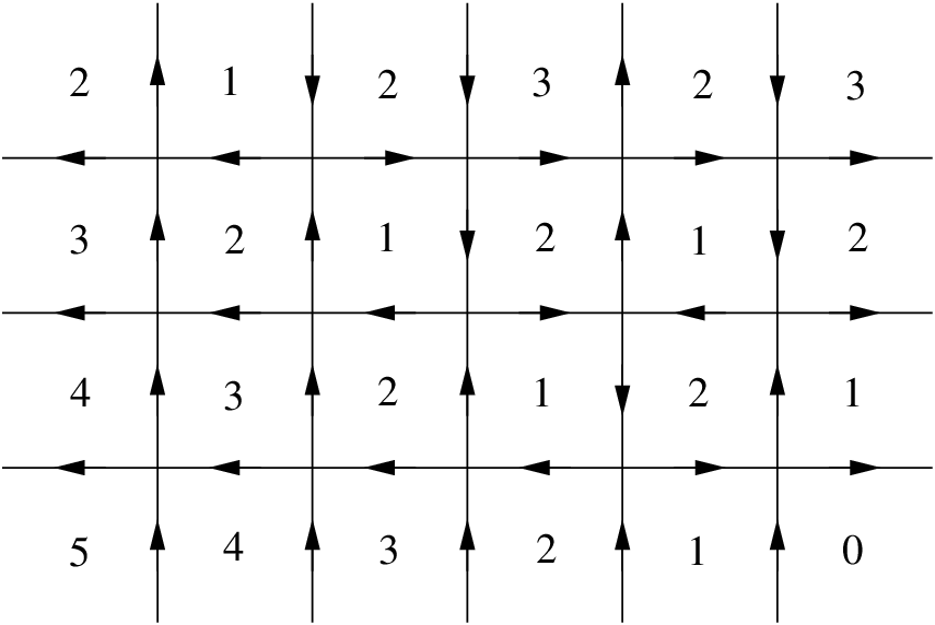
Figure 4. The height function.

To prove the last equation in (1.3), fix a configuration σ\sigma and consider the corresponding height function h⁡(v)h(v) defined on the faces of the lattice (or on the vertices of the dual lattice V′V^{\prime}) by the condition that for any two neighboring faces v,wv,w,

h⁡(w)−h⁡(v)=(−1)s,h(w)-h(v)=(-1)^{s}, (A.1)

where s=0s=0 if the arrow σe\sigma_{e} on the edge e∈Ee\in E, crossing the segment [v,w][v,w], is oriented in such a way that it points from left to right with respect to the vector v​w→\vec{vw} , and s=1s=1 if σe\sigma_{e} is oriented from right to left with respect to v​w→\vec{vw}. The ice-rule ensures that the height function h=hσh=h_{\sigma} exists for any configuration σ\sigma. An example of a configuration and its corresponding height function is given in Figure 4. The height function is defined up to an additive constant, and we fixed it by assigning 0 to the face in the right lower corner. Observe that due to the partial domain wall boundary conditions, on the boundary the height function is linear on the left and right sides, and on the lower boundary. Introduce the coordinates on the dual lattice such that the origin is at the right lower corner, and the xx-axis going left and the yy-axis going up. Then on the left and right sides, and on the lower boundary,

h(0,k)=k,0≤k≤n−m,\displaystyle h(0,k)=k,\quad 0\leq k\leq n-m, (A.2)
h(j,0)=j,0≤j≤n,\displaystyle h(j,0)=j,\quad 0\leq j\leq n,
h(n,k)=n−k,0≤k≤n−m.\displaystyle h(n,k)=n-k,\quad 0\leq k\leq n-m.

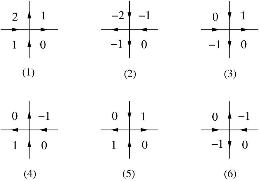
The height function can be used to calculate the differences N2​(σ)−N1​(σ)N_{2}(\sigma)-N_{1}(\sigma) and N4​(σ)−N3​(σ)N_{4}(\sigma)-N_{3}(\sigma). Consider any line LL on the dual lattice parallel to the diagonal y=xy=x. Then along this line the height function jumps by 2 on any vertex configuration of type 1 and by (−2)(-2) on any vertex configuration of type 2. The height function does not change on any vertex configuration of types 3, 4, 5, 6 (See Figure 5).
Refer to caption
Figure 5. The height function on vertex arrow configurations.

Let v1,…,vkv_{1},\ldots,v_{k} be the vertices of the dual lattice V′V^{\prime} along the line LL. Then

h⁡(vk)−h⁡(v1)=2​N1​(σ,L)−2​N2​(σ,L),h(v_{k})-h(v_{1})=2N_{1}(\sigma,L)-2N_{2}(\sigma,L), (A.3)

where Ni​(σ,L)N_{i}(\sigma;L) is the number of vertex states of type ii in σ\sigma on the line LL. By summing up over all possible lines LL, we obtain that

H−S=2​N1​(σ)−2​N2​(σ),H-S=2N_{1}(\sigma)-2N_{2}(\sigma), (A.4)

where HH is the sum of the heights h⁡(v)h(v) along the top row,

H=h⁡(1,n−m)+h⁡(2,n−m)+⋯+h⁡(n−1,n−m).H=h(1,n-m)+h(2,n-m)+\cdots+h(n-1,n-m). (A.5)

and

S\displaystyle S =[1+⋯+(n−m−1)]+[1+⋯+(m−1)]\displaystyle=[1+\cdots+(n-m-1)]+[1+\cdots+(m-1)] (A.6)
=(n−m−1)​(n−m)2+(m−1)​m2.\displaystyle=\frac{(n-m-1)(n-m)}{2}+\frac{(m-1)m}{2}\,.

Similarly, summing up along the lines parallel to the diagonal y=−xy=-x, we obtain that

H−T=2​N3​(σ)−2​N4​(σ),H-T=2N_{3}(\sigma)-2N_{4}(\sigma), (A.7)

where

T\displaystyle T =[(m+1)+⋯+n]+[(n−1)+⋯+(n−m+1)]\displaystyle=[(m+1)+\cdots+n]+[(n-1)+\cdots+(n-m+1)] (A.8)
=(n−m)​(n+m+1)2+(m−1)​(2​n−m)2.\displaystyle=\frac{(n-m)(n+m+1)}{2}+\frac{(m-1)(2n-m)}{2}\,.

Since

T−S=2​m​(n−m),T-S=2m(n-m), (A.9)

we obtain from (A.4) and (A.7) that

[N1​(σ)−N2​(σ)]−[N3​(σ)−N4​(σ)]=T−S2=m⁡(n−m).[N_{1}(\sigma)-N_{2}(\sigma)]-[N_{3}(\sigma)-N_{4}(\sigma)]=\frac{T-S}{2}=m(n-m). (A.10)

This proves the last equation in (1.3).

Appendix B Proof of proposition 2.1

We begin with a partially inhomogeneous six-vertex model with DWBC. That is, consider the n×nn\times n square lattice with parameters (λ1,…,λn)(\lambda_{1},\dots,\lambda_{n}) assigned to horizontal lines from top to bottom, see Fig. 6.

Refer to caption
Figure 6. The n×nn\times n square lattice with spectral parameters (λ1,…,λn)(\lambda_{1},\dots,\lambda_{n}).

We label the six vertex types as in Fig. 1, and use different weights in each row:

wj={a−​(λj):⁣=e−γ​a​(λj)if vertex in row ​j​ is of type 1a+​(λj):⁣=eγ​a​(λj)if vertex in row ​j​ is of type 2b−​(λj):⁣=e−γ​b​(λj)if vertex in row ​j​ is of type 3b+​(λj):⁣=eγ​b​(λj)if vertex in row ​j​ is of type 4c⁡(λj):⁣=sinh⁡(2​γ)if vertex in row ​j​ is of type 5 or 6,w_{j}=\left\{\begin{aligned} &a_{-}(\lambda_{j})&:=&e^{-\gamma}a(\lambda_{j})\qquad&\textrm{if vertex in row }j\textrm{ is of type 1}\\ &a_{+}(\lambda_{j})&:=&e^{\gamma}a(\lambda_{j})\qquad&\textrm{if vertex in row }j\textrm{ is of type 2}\\ &b_{-}(\lambda_{j})&:=&e^{-\gamma}b(\lambda_{j})\qquad&\textrm{if vertex in row }j\textrm{ is of type 3}\\ &b_{+}(\lambda_{j})&:=&e^{\gamma}b(\lambda_{j})\qquad&\textrm{if vertex in row }j\textrm{ is of type 4}\\ &c(\lambda_{j})&:=&\sinh(2\gamma)\qquad&\textrm{if vertex in row }j\textrm{ is of type 5 or 6}\,,\end{aligned}\right. (B.1)

where

a⁡(λ)=sinh⁡(λ−γ),b⁡(λ)=sinh⁡(λ+γ),c⁡(λ)≡c=sinh⁡(2​γ).a(\lambda)=\sinh(\lambda-\gamma)\,,\qquad b(\lambda)=\sinh(\lambda+\gamma)\,,\qquad c(\lambda)\equiv c=\sinh(2\gamma). (B.2)

Introduce the notations

φ⁡(λ):\displaystyle\varphi(\lambda): =a⁡(λ)​b​(λ)=sinh⁡(λ−γ)​sinh⁡(λ+γ),\displaystyle=a(\lambda)b(\lambda)=\sinh(\lambda-\gamma)\sinh(\lambda+\gamma)\,, (B.3)
ϕ⁡(λ):\displaystyle\phi(\lambda): =sinh⁡(2​γ)sinh⁡(λ−γ)​sinh⁡(λ+γ).\displaystyle=\frac{\sinh(2\gamma)}{\sinh(\lambda-\gamma)\sinh(\lambda+\gamma)}.

The Izergin-Korepin formula for the partially inhomogeneous partition function is [6], [7]

Zninh=(−1)n⁡(n−1)/2​∏j=1nφ​(λj)n∏j=0n−1j!​∏1≤j<k≤nsinh⁡(λj−λk)​det(ϕ(k−1)​(λj))j,k=1n,Z_{n}^{\textrm{inh}}=\frac{(-1)^{n(n-1)/2}\prod_{j=1}^{n}\varphi(\lambda_{j})^{n}}{\prod_{j=0}^{n-1}j!\prod_{1\leq j<k\leq n}\sinh(\lambda_{j}-\lambda_{k})}\det\big(\phi^{(k-1)}(\lambda_{j})\big)_{j,k=1}^{n}, (B.4)

where ϕ(k)\phi^{(k)} is the kkth derivative of ϕ\phi. Observe that the factor (−1)n⁡(n−1)/2(-1)^{n(n-1)/2} comes from our ordering of sinh⁡(λj−λk)\sinh(\lambda_{j}-\lambda_{k}) in the denominator.

Now introduce the following notations. Let Zn−m,ninhZ_{n-m,n}^{\textrm{inh}} be the partition function for the six-vertex model on the (n−m)×n(n-m)\times n lattice with the parameters (λm+1,…,λn)(\lambda_{m+1},\dots,\lambda_{n}), with arrows pointing out on the left and right boundaries, in on the bottom boundary, and the top boundary free. On the top boundary, there are exactly mm arrows pointing up, and n−mn-m arrows pointing down. For an mm-tuple of integers 1≤k1<k2<⋯<km≤n1\leq k_{1}<k_{2}<\dots<k_{m}\leq n, consider the partially inhomogeneous six-vertex model on the (n−m)×n(n-m)\times n lattice with the following fixed boundary conditions: arrows on left and right boundaries point out, arrows on bottom boundary point in, and the up-pointing arrows on the top boundary are placed k1k_{1}th, k2k_{2}th, …, and kmk_{m}th location from the right. We denote the partition function of this model with parameters (λm+1,…,λn)(\lambda_{m+1},\dots,\lambda_{n}) by Zn−m,ninh​(k1,k2,…,km)Z_{n-m,n}^{\textrm{inh}(k_{1},k_{2},\dots,k_{m})} Clearly then we have

Zn−m,ninh=∑1≤k1<k2<⋯<km≤nZn−m,ninh​(k1,k2,…,km).Z_{n-m,n}^{\textrm{inh}}=\sum_{1\leq k_{1}<k_{2}<\cdots<k_{m}\leq n}Z_{n-m,n}^{\textrm{inh}(k_{1},k_{2},\dots,k_{m})}\,. (B.5)

For what follows, we set Zn,ninh=ZninhZ_{n,n}^{\textrm{inh}}=Z_{n}^{\textrm{inh}}.

Introduce the notation

fr​(γ)=e2​γ​r+e2​γ​(r−2)+e2​γ​(r−4)+⋯+e−2​γ​r=e2​γ​(r+1)−e−2​γ​(r+1)e2​γ−e−2​γ.f_{r}(\gamma)=e^{2\gamma r}+e^{2\gamma(r-2)}+e^{2\gamma(r-4)}+\cdots+e^{-2\gamma r}=\frac{e^{2\gamma(r+1)}-e^{-2\gamma(r+1)}}{e^{2\gamma}-e^{-2\gamma}}\,. (B.6)

The formula for Zn−m,ninhZ_{n-m,n}^{\textrm{inh}} follows from the following inductive lemma.

Lemma B.1.

The partition function Zn−m−1,ninhZ_{n-m-1,n}^{\textrm{inh}} is obtained from Zn−m,ninhZ_{n-m,n}^{\textrm{inh}} via the limit,

Zn−m−1,ninh=2n−1c​fm​(γ)​limλm+1→∞e−(n−1)​λm+1​Zn−m,ninh.Z_{n-m-1,n}^{\textrm{inh}}=\frac{2^{n-1}}{cf_{m}(\gamma)}\lim_{\lambda_{m+1}\to\infty}e^{-(n-1)\lambda_{m+1}}Z_{n-m,n}^{\textrm{inh}}\,. (B.7)
Proof.

For a configuration on the (n−m)×n(n-m)\times n lattice, let us consider the weight of the first row when there is exactly one cc-type vertex in that row. This can happen when there is an up-pointing arrow in the second row of arrows directly below each up-pointing arrow in the first row. The remaining up-pointing arrow in the second row of arrows may be placed anywhere else, and gives the cc-type vertex in the first row of vertices. Counting the weight of the first row of vertices we find

Zn−m,ninh​(k1,k2,…,km)=\displaystyle Z_{n-m,n}^{\textrm{inh}(k_{1},k_{2},\dots,k_{m})}= c[∑1≤l<k1b−(λm+1)l−1a+(λm+1)n−l−mb+(λm+1)mZn−m−1,ninh​(l,k1,k2,…,km)\displaystyle c\,\bigg[\sum_{1\leq l<k_{1}}b_{-}(\lambda_{m+1})^{l-1}a_{+}(\lambda_{m+1})^{n-l-m}b_{+}(\lambda_{m+1})^{m}Z_{n-m-1,n}^{\textrm{inh}(l,k_{1},k_{2},\dots,k_{m})} (B.8)
+∑k1<l<k2b−(λm+1)l−2a−(λm+1)a+(λm+1)n−l−m+1b+(λm+1)m−1Zn−m−1,ninh​(k1,l,k2,…,km)\displaystyle+\sum_{k_{1}<l<k_{2}}b_{-}(\lambda_{m+1})^{l-2}a_{-}(\lambda_{m+1})a_{+}(\lambda_{m+1})^{n-l-m+1}b_{+}(\lambda_{m+1})^{m-1}Z_{n-m-1,n}^{\textrm{inh}(k_{1},l,k_{2},\dots,k_{m})}
+∑k2<l<k3b−(λm+1)l−3a−(λm+1)2a+(λm+1)n−l−m+2b+(λm+1)m−2Zn−m−1,ninh​(k1,k2,l,k3​…,km)\displaystyle+\sum_{k_{2}<l<k_{3}}b_{-}(\lambda_{m+1})^{l-3}a_{-}(\lambda_{m+1})^{2}a_{+}(\lambda_{m+1})^{n-l-m+2}b_{+}(\lambda_{m+1})^{m-2}Z_{n-m-1,n}^{\textrm{inh}(k_{1},k_{2},l,k_{3}\dots,k_{m})}
⋮\displaystyle\vdots
+∑km−1<l<kmb−(λm+1)l−ma−(λm+1)m−1a+(λm+1)n−l−1b+(λm+1)Zn−m−1,ninh​(k1,…,km−1,l,km)\displaystyle+\sum_{k_{m-1}<l<k_{m}}b_{-}(\lambda_{m+1})^{l-m}a_{-}(\lambda_{m+1})^{m-1}a_{+}(\lambda_{m+1})^{n-l-1}b_{+}(\lambda_{m+1})Z_{n-m-1,n}^{\textrm{inh}(k_{1},\dots,k_{m-1},l,k_{m})}
+∑km<l≤nb−(λm+1)l−m−1a−(λm+1)ma+(λm+1)n−lZn−m−1,ninh​(k1,k2,…,km,l)]\displaystyle+\sum_{k_{m}<l\leq n}b_{-}(\lambda_{m+1})^{l-m-1}a_{-}(\lambda_{m+1})^{m}a_{+}(\lambda_{m+1})^{n-l}Z_{n-m-1,n}^{\textrm{inh}(k_{1},k_{2},\dots,k_{m},l)}\bigg]
+weights of configurations with more than one ​c​-type vertex in first row.\displaystyle+\textrm{weights of configurations with more than one }c\textrm{-type vertex in first row}\,.

Now consider the limit as λm+1→+∞\lambda_{m+1}\to+\infty. In this limit we have

a+(λm+1)=eλm+12(1+𝒪(e−2​λm+1)),a−(λm+1)=eλm+1​e−2​γ2(1+𝒪(e−2​λm+1)),\displaystyle a_{+}(\lambda_{m+1})=\frac{e^{\lambda_{m+1}}}{2}\left(1+{\mathcal{O}}(e^{-2\lambda_{m+1}})\right)\,,\quad a_{-}(\lambda_{m+1})=\frac{e^{\lambda_{m+1}}e^{-2\gamma}}{2}\left(1+{\mathcal{O}}(e^{-2\lambda_{m+1}})\right)\,, (B.9)
b+(λm+1)=eλm+1​e2​γ2(1+𝒪(e−2​λm+1)),b−(λm+1)=eλm+12(1+𝒪(e−2​λm+1)),\displaystyle b_{+}(\lambda_{m+1})=\frac{e^{\lambda_{m+1}}e^{2\gamma}}{2}\left(1+{\mathcal{O}}\left(e^{-2\lambda_{m+1}}\right)\right)\,,\quad b_{-}(\lambda_{m+1})=\frac{e^{\lambda_{m+1}}}{2}\left(1+{\mathcal{O}}\left(e^{-2\lambda_{m+1}}\right)\right)\,,

and configurations with more than one cc-type vertex in the first row are 𝒪⁡(e(n−2)​λm+1){\mathcal{O}}(e^{(n-2)\lambda_{m+1}}). We therefore find

Zn−m,ninh​(k1,k2,…,km)\displaystyle Z_{n-m,n}^{\textrm{inh}(k_{1},k_{2},\dots,k_{m})} =e(n−1)​λm+1​c2n−1[e2​m​γ∑1≤l<k1Zn−m−1,ninh​(l,k1,k2,…,km)\displaystyle=\frac{e^{(n-1)\lambda_{m+1}}\,c}{2^{n-1}}\bigg[e^{2m\gamma}\sum_{1\leq l<k_{1}}Z_{n-m-1,n}^{\textrm{inh}(l,k_{1},k_{2},\dots,k_{m})} (B.10)
+e2​(m−2)​γ∑k1<l<k2Zn−m−1,ninh​(k1,l,k2,…,km)+…\displaystyle+e^{2(m-2)\gamma}\sum_{k_{1}<l<k_{2}}Z_{n-m-1,n}^{\textrm{inh}(k_{1},l,k_{2},\dots,k_{m})}+\quad\dots
+e−2​(m−2)​γ∑km−1<l<kmZn−m−1,ninh​(k1,k2,…,km−1,l,km)\displaystyle+e^{-2(m-2)\gamma}\sum_{k_{m-1}<l<k_{m}}Z_{n-m-1,n}^{\textrm{inh}(k_{1},k_{2},\dots,k_{m-1},l,k_{m})}
+e−2​m​γ∑km<l≤nZn−m−1,ninh​(k1,k2,…,km−1,km,l)](1+𝒪(e−λm+1)).\displaystyle+e^{-2m\gamma}\sum_{k_{m}<l\leq n}Z_{n-m-1,n}^{\textrm{inh}(k_{1},k_{2},\dots,k_{m-1},k_{m},l)}\bigg](1+{\mathcal{O}}(e^{-\lambda_{m+1}}))\,.

Taking the sum over all ordered mm-tuples 1≤k1<k2<⋯<km≤n1\leq k_{1}<k_{2}<\dots<k_{m}\leq n, we find

∑1≤k1<k2<⋯<km≤nZn−m,ninh​(k1,k2,…,km)=e(n−1)​λm+1​c2n−1\displaystyle\sum_{1\leq k_{1}<k_{2}<\cdots<k_{m}\leq n}Z_{n-m,n}^{\textrm{inh}(k_{1},k_{2},\dots,k_{m})}=\frac{e^{(n-1)\lambda_{m+1}}\,c}{2^{n-1}} (B.11)
×[e2​m​γ∑1≤k1<k2<⋯<km≤n∑1≤l<k1Zn−m−1,ninh​(l,k1,k2,…,km)\displaystyle\times\bigg[e^{2m\gamma}\sum_{1\leq k_{1}<k_{2}<\cdots<k_{m}\leq n}\;\sum_{1\leq l<k_{1}}Z_{n-m-1,n}^{\textrm{inh}(l,k_{1},k_{2},\dots,k_{m})}
+e2​(m−2)​γ∑1≤k1<k2<⋯<km≤n∑k1<l<k2Zn−m−1,ninh​(k1,l,k2,…,km)+…\displaystyle+e^{2(m-2)\gamma}\sum_{1\leq k_{1}<k_{2}<\cdots<k_{m}\leq n}\;\sum_{k_{1}<l<k_{2}}Z_{n-m-1,n}^{\textrm{inh}(k_{1},l,k_{2},\dots,k_{m})}+\quad\dots
+e−2​(m−2)​γ∑1≤k1<k2<⋯<km≤n∑km−1<l<kmZn−m−1,ninh​(k1,k2,…,km−1,l,km)\displaystyle+e^{-2(m-2)\gamma}\sum_{1\leq k_{1}<k_{2}<\cdots<k_{m}\leq n}\;\sum_{k_{m-1}<l<k_{m}}Z_{n-m-1,n}^{\textrm{inh}(k_{1},k_{2},\dots,k_{m-1},l,k_{m})}
+e−2​m​γ∑1≤k1<k2<⋯<km≤n∑km<l≤nZn−m−1,ninh​(k1,k2,…,km−1,km,l)](1+𝒪(e−λm+1)).\displaystyle+e^{-2m\gamma}\sum_{1\leq k_{1}<k_{2}<\cdots<k_{m}\leq n}\;\sum_{k_{m}<l\leq n}Z_{n-m-1,n}^{\textrm{inh}(k_{1},k_{2},\dots,k_{m-1},k_{m},l)}\bigg](1+{\mathcal{O}}(e^{-\lambda_{m+1}}))\,.

By (B.5), the left-hand side of the latter equation is equal to Zn−m,ninhZ_{n-m,n}^{\textrm{inh}}. Also, by (B.5),

∑1≤k1<k2<⋯<km≤n∑1≤l<k1Zn−m−1,ninh​(l,k1,k2,…,km)\displaystyle\sum_{1\leq k_{1}<k_{2}<\cdots<k_{m}\leq n}\;\sum_{1\leq l<k_{1}}Z_{n-m-1,n}^{\textrm{inh}(l,k_{1},k_{2},\dots,k_{m})} (B.12)
=∑1≤k1<k2<⋯<km≤n∑k1<l<k2Zn−m−1,ninh​(k1,l,k2,…,km)=…\displaystyle=\sum_{1\leq k_{1}<k_{2}<\cdots<k_{m}\leq n}\;\sum_{k_{1}<l<k_{2}}Z_{n-m-1,n}^{\textrm{inh}(k_{1},l,k_{2},\dots,k_{m})}=\ldots
=∑1≤k1<k2<⋯<km≤n∑km−1<l<kmZn−m−1,ninh​(k1,k2,…,km−1,l,km)\displaystyle=\sum_{1\leq k_{1}<k_{2}<\cdots<k_{m}\leq n}\;\sum_{k_{m-1}<l<k_{m}}Z_{n-m-1,n}^{\textrm{inh}(k_{1},k_{2},\dots,k_{m-1},l,k_{m})}
=∑1≤k1<k2<⋯<km≤n∑km<l≤nZn−m−1,ninh​(k1,k2,…,km−1,km,l)=Zn−m−1,ninh,\displaystyle=\sum_{1\leq k_{1}<k_{2}<\cdots<k_{m}\leq n}\;\sum_{k_{m}<l\leq n}Z_{n-m-1,n}^{\textrm{inh}(k_{1},k_{2},\dots,k_{m-1},k_{m},l)}=Z_{n-m-1,n}^{\textrm{inh}},

hence from (B.11) we obtain that

Zn−m,ninh=e(n−1)​λm+1​c2n−1​Zn−m−1,ninh​fm​(γ)​(1+𝒪⁡(e−λm+1)),Z_{n-m,n}^{\textrm{inh}}=\frac{e^{(n-1)\lambda_{m+1}}\,c}{2^{n-1}}Z_{n-m-1,n}^{\textrm{inh}}f_{m}(\gamma)(1+{\mathcal{O}}(e^{-\lambda_{m+1}}))\,, (B.13)

Taking the limit as λm+1→∞\lambda_{m+1}\to\infty, we obtain (B.7), and lemma B.1 is proved. ∎

Remark: Notice that the coefficient of each of the fixed-boundary partition functions on the right-hand side of (B.10) does not depend on ll, even though the analogous coefficients in (B.8) (before taking λm+1→∞\lambda_{m+1}\to\infty) do depend on ll. This is a consequence of the particular asymptotics (B.9), which in turn follow from the particular choice of weights (B.1). If we let a±​(λj)=a⁡(λj)​e±ηa_{\pm}(\lambda_{j})=a(\lambda_{j})e^{\pm\eta} and b±​(λj)=b⁡(λj)​e±ηb_{\pm}(\lambda_{j})=b(\lambda_{j})e^{\pm\eta} for η≠γ\eta\neq\gamma (see (1.12)), then the ll-dependence of these coefficients persists in (B.10). In this case the multi-sums on the right-hand side of (B.11) do not yield the pDWBC partition function.

We can apply this lemma inductively, starting from

Zn,ninh≡Zninh=(−1)n⁡(n−1)/2​∏j=1nφ​(λj)n∏j=0n−1j!​∏1≤j<k≤nsinh⁡(λj−λk)​det(ϕ(k−1)​(λj))j,k=1n.Z_{n,n}^{\textrm{inh}}\equiv Z_{n}^{\textrm{inh}}=\frac{(-1)^{n(n-1)/2}\prod_{j=1}^{n}\varphi(\lambda_{j})^{n}}{\prod_{j=0}^{n-1}j!\prod_{1\leq j<k\leq n}\sinh(\lambda_{j}-\lambda_{k})}\det\big(\phi^{(k-1)}(\lambda_{j})\big)_{j,k=1}^{n}\,. (B.14)

Namely, we have the following proposition:

Proposition B.2.

The partition function Zn−m,ninhZ_{n-m,n}^{\textrm{inh}} is given by

Zn−m,ninh=\displaystyle Z_{n-m,n}^{\textrm{inh}}= (−1)n⁡(n−1)/2​∏j=m+1n[em​λj​φ​(λj)n]2m⁡(m−1)/2​∏j=0n−1j!​∏m+1≤j<k≤nsinh⁡(λj−λk)\displaystyle\frac{(-1)^{n(n-1)/2}\prod_{j=m+1}^{n}\big[e^{m\lambda_{j}}\varphi(\lambda_{j})^{n}\big]}{2^{m(m-1)/2}\prod_{j=0}^{n-1}j!\prod_{m+1\leq j<k\leq n}\sinh(\lambda_{j}-\lambda_{k})} (B.15)
×det(1(−2)(−2)2…(−2)n−1⋱1(−2​m)(−2​m)2…(−2​m)n−1ϕ⁡(λm+1)ϕ′​(λm+1)ϕ′′​(λm+1)…ϕ(n−1)​(λm+1)⋱ϕ⁡(λn)ϕ′​(λn)ϕ′′​(λn)…ϕ(n−1)​(λn)).\displaystyle\times\det\begin{pmatrix}1&(-2)&(-2)^{2}&\dots&(-2)^{n-1}\\ \vdots&\vdots&\vdots&\ddots&\vdots\\ 1&(-2m)&(-2m)^{2}&\dots&(-2m)^{n-1}\\ \phi(\lambda_{m+1})&\phi^{\prime}(\lambda_{m+1})&\phi^{\prime\prime}(\lambda_{m+1})&\dots&\phi^{(n-1)}(\lambda_{m+1})\\ \vdots&\vdots&\vdots&\ddots&\vdots\\ \phi(\lambda_{n})&\phi^{\prime}(\lambda_{n})&\phi^{\prime\prime}(\lambda_{n})&\dots&\phi^{(n-1)}(\lambda_{n})\end{pmatrix}.
Proof.

From (B.14),

limλ1→∞e−(n−1)​λ1​Zn,ninh\displaystyle\lim_{\lambda_{1}\to\infty}e^{-(n-1)\lambda_{1}}Z_{n,n}^{\textrm{inh}} =limλ1→∞(−1)n⁡(n−1)/2​e−(n−1)​λ1​∏j=1nφ​(λj)n∏j=0n−1j!​∏1≤j<k≤nsinh⁡(λj−λk)\displaystyle=\lim_{\lambda_{1}\to\infty}\frac{(-1)^{n(n-1)/2}e^{-(n-1)\lambda_{1}}\prod_{j=1}^{n}\varphi(\lambda_{j})^{n}}{\prod_{j=0}^{n-1}j!\prod_{1\leq j<k\leq n}\sinh(\lambda_{j}-\lambda_{k})} (B.16)
×det(ϕ⁡(λ1)ϕ′​(λ1)ϕ′′​(λ1)…ϕ(n−1)​(λ1)ϕ⁡(λ2)ϕ′​(λ2)ϕ′′​(λ2)…ϕ(n−1)​(λ2)⋱ϕ⁡(λn)ϕ′​(λn)ϕ′′​(λn)…ϕ(n−1)​(λn)).\displaystyle\times\det\begin{pmatrix}\phi(\lambda_{1})&\phi^{\prime}(\lambda_{1})&\phi^{\prime\prime}(\lambda_{1})&\dots&\phi^{(n-1)}(\lambda_{1})\\ \phi(\lambda_{2})&\phi^{\prime}(\lambda_{2})&\phi^{\prime\prime}(\lambda_{2})&\dots&\phi^{(n-1)}(\lambda_{2})\\ \vdots&\vdots&\vdots&\ddots&\vdots\\ \phi(\lambda_{n})&\phi^{\prime}(\lambda_{n})&\phi^{\prime\prime}(\lambda_{n})&\dots&\phi^{(n-1)}(\lambda_{n})\end{pmatrix}.

Notice that as λj→∞\lambda_{j}\to\infty,

φ⁡(λj)=sinh⁡(λj−γ)​sinh⁡(λj+γ)=e2​λj4​(1+𝒪⁡(e−2​λj)),\displaystyle\varphi(\lambda_{j})=\sinh(\lambda_{j}-\gamma)\sinh(\lambda_{j}+\gamma)=\frac{e^{2\lambda_{j}}}{4}\left(1+{\mathcal{O}}(e^{-2\lambda_{j}})\right)\,, (B.17)
sinh⁡(λj−λk)=eλj−λk2​(1+𝒪⁡(e−2​λj)).\displaystyle\sinh(\lambda_{j}-\lambda_{k})=\frac{e^{\lambda_{j}-\lambda_{k}}}{2}\left(1+{\mathcal{O}}(e^{-2\lambda_{j}})\right).

Consider now

ϕ⁡(λj)\displaystyle\phi(\lambda_{j}) =sinh⁡(2​γ)sinh⁡(λj−γ)​sinh⁡(λj+γ)=4​sinh⁡(2​γ)(eλj−γ−e−λj+γ)​(eλj+γ−e−λj−γ)\displaystyle=\frac{\sinh(2\gamma)}{\sinh(\lambda_{j}-\gamma)\sinh(\lambda_{j}+\gamma)}=\frac{4\sinh(2\gamma)}{\big(e^{\lambda_{j}-\gamma}-e^{-\lambda_{j}+\gamma}\big)\big(e^{\lambda_{j}+\gamma}-e^{-\lambda_{j}-\gamma}\big)} (B.18)
=4​sinh⁡(2​γ)e2​λj​(e−2​γ−e−2​λj)​(e2​γ−e−2​λj)\displaystyle=\frac{4\sinh(2\gamma)}{e^{2\lambda_{j}}\big(e^{-2\gamma}-e^{-2\lambda_{j}}\big)\big(e^{2\gamma}-e^{-2\lambda_{j}}\big)}
=4​sinh⁡(2​γ)e2​λj​(e2​γ−e−2​γ)​(1e−2​γ−e−2​λj−1e2​γ−e−2​λj)\displaystyle=\frac{4\sinh(2\gamma)}{e^{2\lambda_{j}}\big(e^{2\gamma}-e^{-2\gamma}\big)}\left(\frac{1}{e^{-2\gamma}-e^{-2\lambda_{j}}}-\frac{1}{e^{2\gamma}-e^{-2\lambda_{j}}}\right)
=4​sinh⁡(2​γ)(e2​γ−e−2​γ)​∑q=1∞(e2​q​γ−e−2​q​γ)​e−2​q​λj=4​sinh⁡(2​γ)​∑r=0∞fr​(γ)​e−2​(r+1)​λj,\displaystyle=\frac{4\sinh(2\gamma)}{\big(e^{2\gamma}-e^{-2\gamma}\big)}\sum_{q=1}^{\infty}\left(e^{2q\gamma}-e^{-2q\gamma}\right)e^{-2q\lambda_{j}}=4\sinh(2\gamma)\sum_{r=0}^{\infty}f_{r}(\gamma)e^{-2(r+1)\lambda_{j}},

where fr​(γ)f_{r}(\gamma) is defined in (B.6) (we set q=r+1q=r+1 in the last line). Differentiating kk times, we obtain that

ϕ(k)​(λj)\displaystyle\phi^{(k)}(\lambda_{j}) =4​sinh⁡(2​γ)​∑r=0∞fr​(γ)​[−2​(r+1)]k​e−2​(r+1)​λj,\displaystyle=4\sinh(2\gamma)\sum_{r=0}^{\infty}f_{r}(\gamma)[-2(r+1)]^{k}e^{-2(r+1)\lambda_{j}}, (B.19)

Keeping the term r=0r=0 only and taking j=1j=1, we have that

ϕ(k)​(λ1)\displaystyle\phi^{(k)}(\lambda_{1}) =4​sinh⁡(2​γ)​f0​(γ)​(−2)k​e−2​λ1+𝒪⁡(e−4​λ1).\displaystyle=4\sinh(2\gamma)f_{0}(\gamma)(-2)^{k}e^{-2\lambda_{1}}+{\mathcal{O}}(e^{-4\lambda_{1}}). (B.20)

Substituting the latter formula into (B.16), we obtain that

limλ1→∞e−(n−1)​λ1​Zninh\displaystyle\lim_{\lambda_{1}\to\infty}e^{-(n-1)\lambda_{1}}Z_{n}^{\textrm{inh}} =limλ1→∞(−1)n⁡(n−1)/2​4​sinh⁡(2​γ)​f0​(γ)​e−(n+1)​λ1​∏j=1nφ​(λj)n∏j=0n−1j!​∏1≤j<k≤nsinh⁡(λj−λk)\displaystyle=\lim_{\lambda_{1}\to\infty}\frac{(-1)^{n(n-1)/2}4\sinh(2\gamma)f_{0}(\gamma)\,e^{-(n+1)\lambda_{1}}\prod_{j=1}^{n}\varphi(\lambda_{j})^{n}}{\prod_{j=0}^{n-1}j!\prod_{1\leq j<k\leq n}\sinh(\lambda_{j}-\lambda_{k})} (B.21)
×det(1(−2)(−2)2…(−2)n−1ϕ⁡(λ2)ϕ′​(λ2)ϕ′′​(λ2)…ϕ(n−1)​(λ2)⋱ϕ⁡(λn)ϕ′​(λn)ϕ′′​(λn)…ϕ(n−1)​(λn)).\displaystyle\times\det\begin{pmatrix}1&(-2)&(-2)^{2}&\dots&(-2)^{n-1}\\ \phi(\lambda_{2})&\phi^{\prime}(\lambda_{2})&\phi^{\prime\prime}(\lambda_{2})&\dots&\phi^{(n-1)}(\lambda_{2})\\ \vdots&\vdots&\vdots&\ddots&\vdots\\ \phi(\lambda_{n})&\phi^{\prime}(\lambda_{n})&\phi^{\prime\prime}(\lambda_{n})&\dots&\phi^{(n-1)}(\lambda_{n})\end{pmatrix}.

Now, from (B.17) we find that

limλ1→∞e−(n+1)​λ1​φ​(λ1)n∏k=2nsinh⁡(λ1−λk)\displaystyle\lim_{\lambda_{1}\to\infty}\frac{e^{-(n+1)\lambda_{1}}\varphi(\lambda_{1})^{n}}{\prod_{k=2}^{n}\sinh(\lambda_{1}-\lambda_{k})} =limλ1→∞e−(n+1)​λ1​(e2​λ14)n∏k=2neλ1−λk2=12n+1​∏k=2neλk,\displaystyle=\lim_{\lambda_{1}\to\infty}\frac{e^{-(n+1)\lambda_{1}}\left(\frac{e^{2\lambda_{1}}}{4}\right)^{n}}{\prod_{k=2}^{n}\frac{e^{\lambda_{1}-\lambda_{k}}}{2}}=\frac{1}{2^{n+1}}\,\prod_{k=2}^{n}e^{\lambda_{k}}, (B.22)

hence

limλ1→∞e−(n−1)​λ1​Zninh\displaystyle\lim_{\lambda_{1}\to\infty}e^{-(n-1)\lambda_{1}}Z_{n}^{\textrm{inh}} =(−1)n⁡(n−1)/2​sinh⁡(2​γ)​f0​(γ)​∏j=2n[eλj​φ​(λj)n]2n−1​∏j=0n−1j!​∏2≤j<k≤nsinh⁡(λj−λk)\displaystyle=\frac{(-1)^{n(n-1)/2}\sinh(2\gamma)f_{0}(\gamma)\prod_{j=2}^{n}\left[e^{\lambda_{j}}\varphi(\lambda_{j})^{n}\right]}{2^{n-1}\prod_{j=0}^{n-1}j!\prod_{2\leq j<k\leq n}\sinh(\lambda_{j}-\lambda_{k})} (B.23)
×det(1(−2)(−2)2…(−2)n−1ϕ⁡(λ2)ϕ′​(λ2)ϕ′′​(λ2)…ϕ(n−1)​(λ2)⋱ϕ⁡(λn)ϕ′​(λn)ϕ′′​(λn)…ϕ(n−1)​(λn)).\displaystyle\times\det\begin{pmatrix}1&(-2)&(-2)^{2}&\dots&(-2)^{n-1}\\ \phi(\lambda_{2})&\phi^{\prime}(\lambda_{2})&\phi^{\prime\prime}(\lambda_{2})&\dots&\phi^{(n-1)}(\lambda_{2})\\ \vdots&\vdots&\vdots&\ddots&\vdots\\ \phi(\lambda_{n})&\phi^{\prime}(\lambda_{n})&\phi^{\prime\prime}(\lambda_{n})&\dots&\phi^{(n-1)}(\lambda_{n})\end{pmatrix}.

Thus, by (B.7) [remind that c=sinh⁡(2​γ)c=\sinh(2\gamma)],

Zn−1,ninh\displaystyle Z_{n-1,n}^{\textrm{inh}} =2n−1c​f0​(γ)​limλ1→∞e−(n−1)​λ1​Zninh=(−1)n⁡(n−1)/2​∏j=2n[eλj​φ​(λj)n]∏j=0n−1j!​∏2≤j<k≤nsinh⁡(λj−λk)\displaystyle=\frac{2^{n-1}}{cf_{0}(\gamma)}\lim_{\lambda_{1}\to\infty}e^{-(n-1)\lambda_{1}}Z_{n}^{\textrm{inh}}=\frac{(-1)^{n(n-1)/2}\prod_{j=2}^{n}\left[e^{\lambda_{j}}\varphi(\lambda_{j})^{n}\right]}{\prod_{j=0}^{n-1}j!\prod_{2\leq j<k\leq n}\sinh(\lambda_{j}-\lambda_{k})} (B.24)
×det(1(−2)(−2)2…(−2)n−1ϕ⁡(λ2)ϕ′​(λ2)ϕ′′​(λ2)…ϕ(n−1)​(λ2)⋱ϕ⁡(λn)ϕ′​(λn)ϕ′′​(λn)…ϕ(n−1)​(λn)).\displaystyle\times\det\begin{pmatrix}1&(-2)&(-2)^{2}&\dots&(-2)^{n-1}\\ \phi(\lambda_{2})&\phi^{\prime}(\lambda_{2})&\phi^{\prime\prime}(\lambda_{2})&\dots&\phi^{(n-1)}(\lambda_{2})\\ \vdots&\vdots&\vdots&\ddots&\vdots\\ \phi(\lambda_{n})&\phi^{\prime}(\lambda_{n})&\phi^{\prime\prime}(\lambda_{n})&\dots&\phi^{(n-1)}(\lambda_{n})\end{pmatrix}.

We now consider the limit of e−(n−1)​λ2​Zn−1,ninhe^{-(n-1)\lambda_{2}}Z_{n-1,n}^{\textrm{inh}} as λ2→∞\lambda_{2}\to\infty. To that end, we keep in (B.19) terms with r=0r=0 and r=1r=1:

ϕ(k)​(λ2)\displaystyle\phi^{(k)}(\lambda_{2}) =4​sinh⁡(2​γ)​[(−2)k​e−2​λ2+f1​(γ)​(−4)k​e−4​λ2]+𝒪⁡(e−6​λ2).\displaystyle=4\sinh(2\gamma)\left[(-2)^{k}e^{-2\lambda_{2}}+f_{1}(\gamma)(-4)^{k}e^{-4\lambda_{2}}\right]+{\mathcal{O}}(e^{-6\lambda_{2}}). (B.25)

Substituting this into the second row of the determinant in (B.24) and taking a linear combination with the first row, we obtain that

limλ2→∞e−(n−1)​λ2\displaystyle\lim_{\lambda_{2}\to\infty}e^{-(n-1)\lambda_{2}} Zn−1,ninh=limλ2→∞(−1)n⁡(n−1)/2​4​sinh⁡(2​γ)​f1​(γ)​e−(n+3)​λ2​∏j=2n[eλj​φ​(λj)n]∏j=0n−1j!​∏2≤j<k≤nsinh⁡(λj−λk)\displaystyle Z_{n-1,n}^{\textrm{inh}}=\lim_{\lambda_{2}\to\infty}\frac{(-1)^{n(n-1)/2}4\sinh(2\gamma)f_{1}(\gamma)e^{-(n+3)\lambda_{2}}\prod_{j=2}^{n}\left[e^{\lambda_{j}}\varphi(\lambda_{j})^{n}\right]}{\prod_{j=0}^{n-1}j!\prod_{2\leq j<k\leq n}\sinh(\lambda_{j}-\lambda_{k})} (B.26)
×det(1(−2)(−2)2…(−2)n−11(−4)(−4)2…(−4)n−1ϕ⁡(λ3)ϕ′​(λ3)ϕ′′​(λ3)…ϕ(n−1)​(λ3)⋱ϕ⁡(λn)ϕ′​(λn)ϕ′′​(λn)…ϕ(n−1)​(λn)).\displaystyle\times\det\begin{pmatrix}1&(-2)&(-2)^{2}&\dots&(-2)^{n-1}\\ 1&(-4)&(-4)^{2}&\dots&(-4)^{n-1}\\ \phi(\lambda_{3})&\phi^{\prime}(\lambda_{3})&\phi^{\prime\prime}(\lambda_{3})&\dots&\phi^{(n-1)}(\lambda_{3})\\ \vdots&\vdots&\vdots&\ddots&\vdots\\ \phi(\lambda_{n})&\phi^{\prime}(\lambda_{n})&\phi^{\prime\prime}(\lambda_{n})&\dots&\phi^{(n-1)}(\lambda_{n})\end{pmatrix}.

Now,

limλ2→∞e−(n+3)​λ2​[eλ2​φ​(λ2)n]∏k=3nsinh⁡(λ2−λk)\displaystyle\lim_{\lambda_{2}\to\infty}\frac{e^{-(n+3)\lambda_{2}}\left[e^{\lambda_{2}}\varphi(\lambda_{2})^{n}\right]}{\prod_{k=3}^{n}\sinh(\lambda_{2}-\lambda_{k})} =limλ2→∞e−(n+2)​λ2​(e2​λ24)n∏k=3neλ2−λk2=12n+2​∏k=3neλk,\displaystyle=\lim_{\lambda_{2}\to\infty}\frac{e^{-(n+2)\lambda_{2}}\left(\frac{e^{2\lambda_{2}}}{4}\right)^{n}}{\prod_{k=3}^{n}\frac{e^{\lambda_{2}-\lambda_{k}}}{2}}=\frac{1}{2^{n+2}}\,\prod_{k=3}^{n}e^{\lambda_{k}}, (B.27)

hence

limλ2→∞e−(n−1)​λ2\displaystyle\lim_{\lambda_{2}\to\infty}e^{-(n-1)\lambda_{2}} Zn−1,ninh=(−1)n⁡(n−1)/2​sinh⁡(2​γ)​f1​(γ)​∏j=3n[e2​λj​φ​(λj)n]2n​∏j=0n−1j!​∏3≤j<k≤nsinh⁡(λj−λk)\displaystyle Z_{n-1,n}^{\textrm{inh}}=\frac{(-1)^{n(n-1)/2}\sinh(2\gamma)f_{1}(\gamma)\prod_{j=3}^{n}\left[e^{2\lambda_{j}}\varphi(\lambda_{j})^{n}\right]}{2^{n}\prod_{j=0}^{n-1}j!\prod_{3\leq j<k\leq n}\sinh(\lambda_{j}-\lambda_{k})} (B.28)
×det(1(−2)(−2)2…(−2)n−11(−4)(−4)2…(−4)n−1ϕ⁡(λ3)ϕ′​(λ3)ϕ′′​(λ3)…ϕ(n−1)​(λ3)⋱ϕ⁡(λn)ϕ′​(λn)ϕ′′​(λn)…ϕ(n−1)​(λn)).\displaystyle\times\det\begin{pmatrix}1&(-2)&(-2)^{2}&\dots&(-2)^{n-1}\\ 1&(-4)&(-4)^{2}&\dots&(-4)^{n-1}\\ \phi(\lambda_{3})&\phi^{\prime}(\lambda_{3})&\phi^{\prime\prime}(\lambda_{3})&\dots&\phi^{(n-1)}(\lambda_{3})\\ \vdots&\vdots&\vdots&\ddots&\vdots\\ \phi(\lambda_{n})&\phi^{\prime}(\lambda_{n})&\phi^{\prime\prime}(\lambda_{n})&\dots&\phi^{(n-1)}(\lambda_{n})\end{pmatrix}.

Thus,

Zn−2,ninh\displaystyle Z_{n-2,n}^{\textrm{inh}} =2n−1c​f1​(γ)​limλ2→∞e−(n−1)​λ1​Zn−1,ninh=(−1)n⁡(n−1)/2​∏j=3n[e2​λj​φ​(λj)n]2​∏j=0n−1j!​∏3≤j<k≤nsinh⁡(λj−λk)\displaystyle=\frac{2^{n-1}}{cf_{1}(\gamma)}\lim_{\lambda_{2}\to\infty}e^{-(n-1)\lambda_{1}}Z_{n-1,n}^{\textrm{inh}}=\frac{(-1)^{n(n-1)/2}\prod_{j=3}^{n}\left[e^{2\lambda_{j}}\varphi(\lambda_{j})^{n}\right]}{2\prod_{j=0}^{n-1}j!\prod_{3\leq j<k\leq n}\sinh(\lambda_{j}-\lambda_{k})} (B.29)
×det(1(−2)(−2)2…(−2)n−11(−4)(−4)2…(−4)n−1ϕ⁡(λ3)ϕ′​(λ3)ϕ′′​(λ3)…ϕ(n−1)​(λ3)⋱ϕ⁡(λn)ϕ′​(λn)ϕ′′​(λn)…ϕ(n−1)​(λn)).\displaystyle\times\det\begin{pmatrix}1&(-2)&(-2)^{2}&\dots&(-2)^{n-1}\\ 1&(-4)&(-4)^{2}&\dots&(-4)^{n-1}\\ \phi(\lambda_{3})&\phi^{\prime}(\lambda_{3})&\phi^{\prime\prime}(\lambda_{3})&\dots&\phi^{(n-1)}(\lambda_{3})\\ \vdots&\vdots&\vdots&\ddots&\vdots\\ \phi(\lambda_{n})&\phi^{\prime}(\lambda_{n})&\phi^{\prime\prime}(\lambda_{n})&\dots&\phi^{(n-1)}(\lambda_{n})\end{pmatrix}.

Continuing in this manner mm times, we arrive at the formula

Zn−m,ninh=\displaystyle Z_{n-m,n}^{\textrm{inh}}= (−1)n⁡(n−1)/2​∏j=m+1n[em​λj​φ​(λj)n]21+2+⋯+(m−1)​∏j=0n−1j!​∏m+1≤j<k≤nsinh⁡(λj−λk)\displaystyle\frac{(-1)^{n(n-1)/2}\prod_{j=m+1}^{n}\big[e^{m\lambda_{j}}\varphi(\lambda_{j})^{n}\big]}{2^{1+2+\cdots+(m-1)}\prod_{j=0}^{n-1}j!\prod_{m+1\leq j<k\leq n}\sinh(\lambda_{j}-\lambda_{k})} (B.30)
×det(1(−2)(−2)2…(−2)n−1⋱1(−2​m)(−2​m)2…(−2​m)n−1ϕ⁡(λm+1)ϕ′​(λm+1)ϕ′′​(λm+1)…ϕ(n−1)​(λm+1)⋱ϕ⁡(λn)ϕ′​(λn)ϕ′′​(λn)…ϕ(n−1)​(λn)),\displaystyle\times\det\begin{pmatrix}1&(-2)&(-2)^{2}&\dots&(-2)^{n-1}\\ \vdots&\vdots&\vdots&\ddots&\vdots\\ 1&(-2m)&(-2m)^{2}&\dots&(-2m)^{n-1}\\ \phi(\lambda_{m+1})&\phi^{\prime}(\lambda_{m+1})&\phi^{\prime\prime}(\lambda_{m+1})&\dots&\phi^{(n-1)}(\lambda_{m+1})\\ \vdots&\vdots&\vdots&\ddots&\vdots\\ \phi(\lambda_{n})&\phi^{\prime}(\lambda_{n})&\phi^{\prime\prime}(\lambda_{n})&\dots&\phi^{(n-1)}(\lambda_{n})\end{pmatrix},

which proves Proposition B.2. ∎

References

  • [1] J. Baik, T. Kriecherbauer, K. T.-R. McLaughlin, and P. D. Miller. Discrete orthogonal polynomials, volume 164 of Annals of Mathematics Studies. Princeton University Press, Princeton, NJ, 2007. Asymptotics and applications.
  • [2] Pavel Bleher and Karl Liechty. Exact solution of the six-vertex model with domain wall boundary conditions. Ferroelectric phase. Comm. Math. Phys., 286(2):777–801, 2009.
  • [3] Pavel Bleher and Karl Liechty. Random matrices and the six-vertex model, volume 32 of CRM Monograph Series. American Mathematical Society, Providence, RI, 2014.
  • [4] Alexei Borodin and Dmitriy Boyarchenko. Distribution of the first particle in discrete orthogonal polynomial ensembles. Comm. Math. Phys., 234(2):287–338, 2003.
  • [5] O. Foda and M. Wheeler. Partial domain wall partition functions. J. High Energy Phys., (7):186, front matter+35, 2012.
  • [6] A. G. Izergin. Partition function of a six-vertex model in a finite volume. Dokl. Akad. Nauk SSSR, 297(2):331–333, 1987.
  • [7] A. G. Izergin, D. A. Coker, and V. E. Korepin. Determinant formula for the six-vertex model. J. Phys. A, 25(16):4315–4334, 1992.
  • [8] Kurt Johansson. Shape fluctuations and random matrices. Comm. Math. Phys., 209(2):437–476, 2000.
  • [9] Roelof Koekoek, Peter A. Lesky, and René F. Swarttouw. Hypergeometric orthogonal polynomials and their qq-analogues. Springer Monographs in Mathematics. Springer-Verlag, Berlin, 2010. With a foreword by Tom H. Koornwinder.
  • [10] V. E. Korepin. Calculation of norms of Bethe wave functions. Comm. Math. Phys., 86(3):391–418, 1982.
  • [11] Ivan Kostov and Yutaka Matsuo. Inner products of Bethe states as partial domain wall partition functions. J. High Energy Phys., (10):168, front matter + 14, 2012.
  • [12] X.-S. Wang and R. Wong. Global asymptotics of the Meixner polynomials. Asymptot. Anal., 75(3-4):211–231, 2011.