Sparse Fast Fourier Transform for Exactly and Generally -Sparse Signals by Downsampling and Sparse Recovery
Abstract
Fast Fourier Transform (FFT) is one of the most important tools in digital signal processing. FFT costs for transforming a signal of length . Recently, Sparse Fourier Transform (SFT) has emerged as a critical issue addressing how to compute a compressed Fourier transform of a signal with complexity being related to the sparsity of its spectrum.
In this paper, a new SFT algorithm is proposed for both exactly -sparse signals (with non-zero frequencies) and generally -sparse signals (with significant frequencies), with the assumption that the distribution of the non-zero frequencies is uniform. The nuclear idea is to downsample the input signal at the beginning; then, subsequent processing operates under downsampled signals, where signal lengths are proportional to . Downsampling, however, possibly leads to “aliasing”. By the shift property of DFT, we recast the aliasing problem as complex Bose-Chaudhuri-Hocquenghem (BCH) codes solved by syndrome decoding. The proposed SFT algorithm for exactly -sparse signals recovers frequencies with computational complexity and probability at least under , where is a user-controlled parameter.
For generally -sparse signals, due to the fact that BCH codes are sensitive to noise, we combine a part of syndrome decoding with a compressive sensing-based solver for obtaining significant frequencies. The computational complexity of our algorithm is , where the Big-O constant of is very small and only a simple operation involves . Our simulations reveal that does not dominate the computational cost of sFFT-DT.
In this paper, we provide mathematical analyses for recovery performance and computational complexity, and conduct comparisons with known SFT algorithms in both aspects of theoretical derivations and simulation results. In particular, our algorithms for both exactly and generally -sparse signals are easy to implement.
Index Terms:
Compressed Sensing, Downsampling, FFT, Sparse FFT, Sparsity.I Introduction
I-A Background and Related Work
Fast Fourier transform (FFT) is one of the most important approaches for fast computing discrete Fourier transform (DFT) of a signal with time complexity , where is the signal length. FFT has been used widely in the communities of signal processing and communications. How to outperform FFT, however, remains a challenge and persistently receives attention.
Sparsity is inherent in signals and has been exploited to speed up FFT in the literature. A signal of length is called exactly -sparse if there are non-zero frequencies with . On the other hand, a signal is called generally -sparse if all frequencies are non-zero but we are only interested in keeping the first -largest (significant) frequencies in terms of magnitudes and ignore the remainder. Instead of computing all frequencies, Sparse Fourier Transform (SFT) has emerged as a critical topic and aim to compute a compressed DFT, where the time complexity is proportional to .
A. C. Gilbert [1] et al. propose an overview of SFT and summarize a common three-stage approach: 1) identify locations of non-zero or significant frequencies; 2) estimate the values of the identified frequencies; and 3) subtract the contribution of the partial Fourier representation computed from the first two stages from the signal and go back to stage 1. Some prior works are briefly described as follows.
M. A. Iwen [2] proposes a sublinear-time SFT algorithm based on Chinese Remainder Theorem (CRT) with computational complexities (a) with a non-uniform failure probability per signal and (b) with a deterministic recovery guarantee. Iwen’s algorithm can work for general with the help of interpolation. Although the algorithm offers strong theoretical analysis, the empirical experiments show that it suffers Big-O constants. For example, in Fig. 5 of [2], it shows to outperform FFTW under and . The approximation error bounds in [2] are further improved in [3].
H. Hassanieh et al. propose so-called Sparse Fast Fourier Transform (sFFT) [4][5]. The idea behind sFFT is to subsample fewer frequencies (proportional to ) since most of frequencies are zero or insignificant. Nevertheless, the difficulty is which frequencies should be subsampled as the locations and values of the non-zero frequencies are unknown. To cope with this difficulty, sFFT utilizes the strategies of filtering and permutation introduced in [6], which can increase the probability of capturing useful information from subsampled frequencies. For exactly -sparse and general -sparse signals, sFFT costs and , respectively. In their simulations, sFFT is faster than FFTW [7] (a very fast C subroutine library for computing FFT) for exactly -sparse signals with .
Even though sFFT [4][5] is outstanding, there are some limitations, summarized as follows: 1) Filtering and permutation are operated on the input signal. These operations are related to . Thus, the complexity of sFFT still involves and cannot achieve the theoretical ideal complexity . 2) sFFT only guarantees that it succeeds with a constant probability (e.g., ). 3) The implementation of sFFT for generally -sparse signals is very complicated as it involves too many parameters that are difficult to set.11 1 In fact, according to our private communication with the authors of [4][5], they would not recommend implementing this code since it is not trivial. The authors also suggest that it is not easy to clearly illustrate which setting will work best because of the constants in the Big-O functions and because of the dependency on the implementation. The authors themselves did not implement it since they believed that the constants would be large and that it would not realize much improvement over FFTW.
Ghazi et al. [8] propose another algorithm based on Prony’s method for exactly -sparse signals. The basic idea is similar to our previous work [9]. The key difference is that Ghazi et al.’s method recovers all non-zero frequencies once, while we propose a top-down strategy to solve non-zero frequencies iteratively. Furthermore, due to different parameter settings and root finding algorithms, Ghazi’s SFT costs along with different big-O constants. The comparison between these two methods in terms of computational complexity and recovery performance will be discussed later in Sec. II-C.
S. Heider et al.’s method [10] combines Prony-like methods with quasi random sampling and band pass filtering. Compared with our method, they estimate the positions and values of non-zero frequencies in each band based on the ESPRIT method instead of syndrome decoding. ESPRIT requires more computational cost resulting in the total complexity being . Their proof also shows that is more strict than in our case for exactly- sparse signal.
Pawar and Ramchandran [11] propose an algorithm, called FFAST (Fast Fourier Aliasing-based Sparse Transform), which focuses on exactly -sparse signals. Their approach is based on filterless downsampling of the input signal using a constant number of co-prime downsampling factors guided by CRT. These aliasing patterns of different downsampled signals are formulated as parity-check constraints of good erasure-correcting sparse-graph codes. FFAST costs but relies on the constraint that co-prime downsampling factors must divide . Moreover, the smallest downsampling factor bounds FFAST’s computational cost. For example, if and , the smallest downsampling factor is . In this case, the computational cost of calculating FFT of a downsampled signal with length is higher than . Actually, these limitations are possibly harsh.
We summarize and compare the SFT algorithms reviewed above in Table I in terms of the number of samples, computational complexity, and assumption regarding sparsity. More specifically, the number of samples decides how much information SFT algorithms require in order to reconstruct -sparse signals. It is especially important for some applications, including Analog-to-Digital converter, which are benefited by low sampling rates. Moreover, the assumption of a certain range of sparsity guarantees that SFT algorithms can have high quality of reconstruction. We can find from Table I that our algorithms have the lowest computational complexity, the lowest number of samples, and the best range of sparsity for exactly -sparse signals. Although the sparsity constraint seems to be more tough for generally -sparse signals in our method, for a (very) sparse signal we still can solve it by assuming that its sparsity is higher than the true one with more computational cost. In the simulations, we show that the Big-O constants for both exactly -sparse and generally -sparse signals are actually small, implying the practicability of our proposed approaches for real implementation.
I-B Our Contributions
In our previous work [9], we propose a SFT algorithm, called sFFT-DT, based on filterless downsampling with time complexity of only for exactly -sparse signals. The idea behind sFFT-DT is to downsample the input signal in the time domain before directly conducting all subsequent operations on the downsampled signals. By choosing an appropriate downsampling factor to make the length of a downsampled signal be , no operations related to are required in sFFT-DT. Downsampling, however, possibly leads to “aliasing,” where different frequencies become indistinguishable in terms of their locations and values. To overcome this problem, the locations and values of these non-zero entries are considered as unknown variables and the “aliasing problem” is reformulated as “Moment Preserving Problem (MPP)”. Furthermore, sFFT-DT is conducted in a manner of a top-down iterative strategy under different downsampling factors, which can efficiently reduce the computational cost. In comparison with other CRT-based approaches [10][11] that require multiple co-prime integers dividing , our method only needs the downsampling factor to divide but does not suffer the co-prime constraint, implying that sFFT-DT has more freedom for .
In this paper, we further examine the accurate computational cost and theoretical performance of sFFT-DT for exactly -sparse signals. We derive the Big-O constants of computational complexity of sFFT-DT and show that they are smaller than those of Ghazi et al.’s sFFT [8]. In addition, sFFT-DT is efficient due to , which makes it useful whatever the sparsity is. Finally, all operations of sFFT-DT are solved via analytical solutions but those of Ghazi et al.’s sFFT involve a numerical root finding algorithm, which is more complicated in terms of hardware implementation.
In the context of SFT, sparsity plays an important role. The performance and computational complexity of previous SFT algorithms [4][5][8][11] have been analyzed based on the assumption that sparsity is known in advance. In practice, however, is unknown and is an input parameter decided by the user. If is not guessed correctly, the performance is degraded and/or the computational overhead is higher than expected because the choice of some parameters depends on . In this paper, we propose a simple solution to address this problem and relax this impractical assumption. We show that the cost for deciding is the same as that required for sFFT-DT with known .
In addition to conducting more advanced theoretical analyses, we also study sFFT-DT for generally -sparse signals in this paper. For generally -sparse signals, since all frequencies are non-zero, each frequency of a downsampled signal is composed of significant and insignificant frequencies due to aliasing. To extract significant components from each frequency, the concept of sparse signal recovered from fewer samples, originating from compressive sensing (CS) [12], is employed since significant entries are “sparse”. A pruning strategy is further used to exclude locations of insignificant terms. We prove the sufficient conditions of robust recovery, which means reconstruction error is bounded, with time complexity under . The empirical experiments show that the Big-O constant of sFFT-DT is small and outperforms FFT when and .
Finally, we conclude that our methods are easy to implement and are demonstrated to outperform the state-of-the-art in terms of theoretical analyses and simulation results.
I-C Organization of This Paper
II sFFT-DT for Exactly -Sparse Signals
We describe the proposed method for exactly -sparse signals and provide analyses for parameter setting, computational complexity, and recovery performance. The proposed method contains three steps.
- 1.
Downsample the original signal in the time domain.
- 2.
Calculate Discrete Fourier Transform (DFT) of the downsampled signal by FFT.
- 3.
Use the DFT of the downsampled signal to locate and estimate non-zero frequencies..
Steps 1 and 2 are simple and straightforward. Thus, we focus on Step 3 here.
Throughout the paper, common notations are defined as follows. Let be the input signal in the time domain, and let be DFT of . is the DFT matrix such that with and .
II-A Problem Formulation
Let be the signal downsampled from an original signal , where , , and integer is a downsampling factor. The length of the downsampled signal is Let be DFT of , where
| (1) |
The objective here is to locate and estimate non-zero frequencies of from .
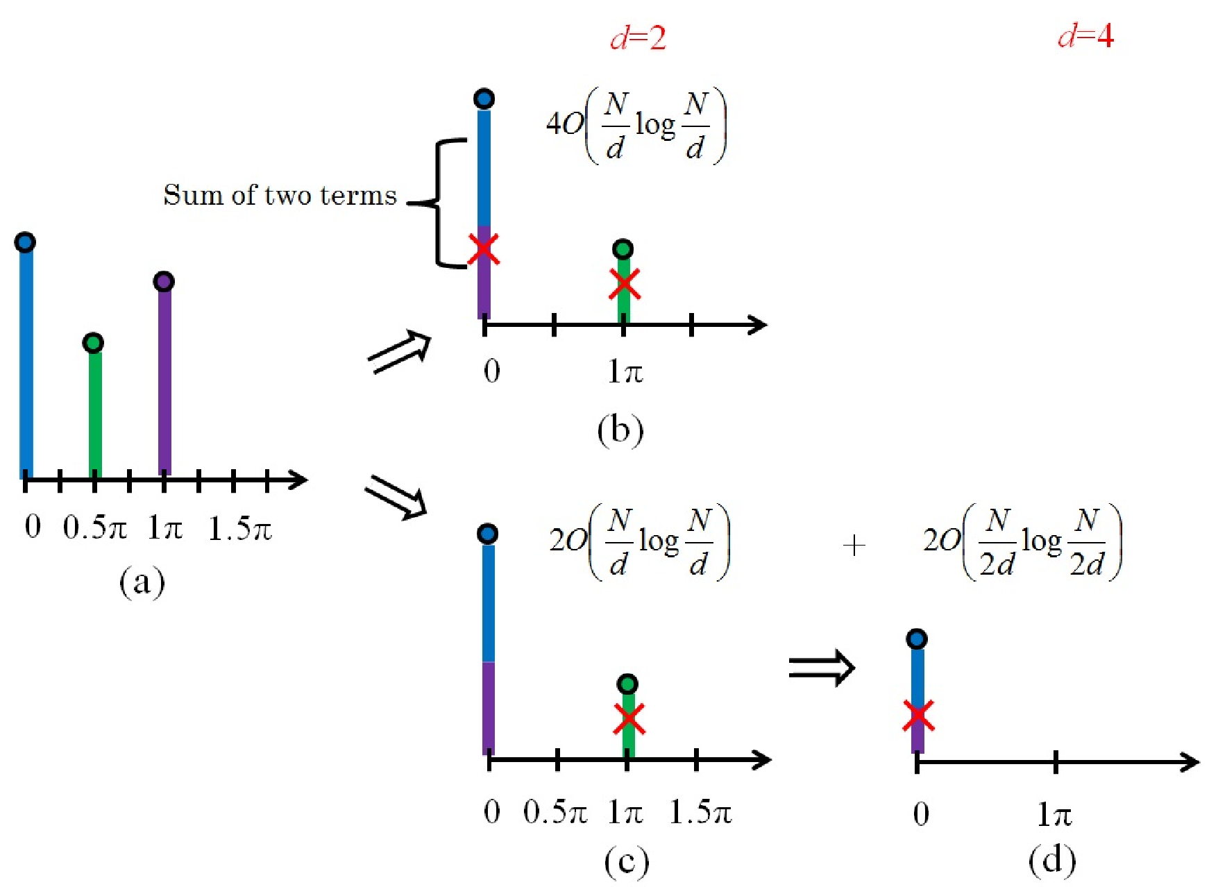
Note that each frequency of is a sum of terms of . When more than two terms of are non-zero, “aliasing” occurs, as illustrated in Fig. 1. Fig. 1(a) shows an original signal in the frequency domain, where only three frequencies are non-zero (appearing at normalized frequencies = , , and ). Fig. 1(b) shows the downsampled signal in the frequency domain when , where the downsampled frequency at incurs aliasing; i.e., the frequency of at collides with the one at . In Fig. 1(b), we solve all non-zero downsampled frequencies once, no matter whether aliasing occurs or not. This procedure is called non-iterative sFFT-DT and will be discussed in detail later. Instead of solving all of the downsampled frequencies once, Fig. 1(c) illustrates an example of iteratively solving frequencies. At the first iteration, the downsampled frequency without aliasing at is solved. This makes the remaining downsampled frequencies more sparse. Then, the signal is downsampled again with . At the second iteration, we solve the downsampled frequency with aliasing at . This procedure, called iterative sFFT-DT, will be discussed further in Sec. II-D.
In the following, we describe how to solve the aliasing problem by introducing the shift property of DFT. Let , where denotes the shift factor. Each frequency of is denoted as:
| (2) |
Thus, Eq. (2) degenerates to Eq. (1) when . In practice, all we can obtain are ’s for different ’s.
For each downsampling factor , there will be no more than terms on the right side of Eq. (2), where each term contains two unknown variables, and . Let , , denote the number of terms on the right side of Eq. (2). Therefore, we need equations to solve these variables, and is within the range of . By taking the above into consideration, the problem of solving the unknown variables on the right side of Eq. (2) can be formulated22 2 In the previous version [9], it is interpreted as a moment preserving problem (MPP). Specifically, solving MPP is equivalent to solving complex BCH codes, where the syndromes produced by partial Fourier transform are consistent with moments. via BCH codes as:
| (3) | ||||
where is known and denoted as while and represent unknown and , respectively, for and . To simplify the notation, we let and .
It is trivial that no aliasing occurs if , irrespective of the downsampling factor. Under this circumstance, we have , , , and , according to Eq. (3). We obtain that and . After some derivations, we can solve and assign at the position . The above solver only works under a non-aliasing environment with . Nevertheless, when aliasing appears (i.e., ), it fails.
II-B Syndrome Decoding
Note that Eq. (3) is nonlinear and cannot be solved by simple linear matrix operations.
On the contrary, we have to solve ’s first, such that Eq. (3) becomes linear.
Then, ’s can be solved by matrix inversion.
Thus, the main difficulty is how to solve ’s given known syndromes.
According to [14], given the unique syndromes with , , …, , there must exist the corresponding orthogonal polynomial equation, , with roots ’s for .
That is, ’s can be obtained as the roots of .
The steps for syndrome decoding are as follows.
Step (i): Let the orthogonal polynomial equation be:
| (4) |
The relationship between and the syndromes is as follows:
| (5) | ||||
Eq. (5) can be formulated as , where , , and .
Thus, Eq. (5) can be solved by matrix inversion to obtain ’s.
Step (ii): Find the roots of in Eq. (4).
These roots are the solutions of , ,…, respectively.
Step (iii): Substitute all ’s into Eq. (3), and solve the resulting equations to obtain ’s.
Tsai [15] showed a complete analytical solution composed of the aforementioned three steps for , based on the constraint that . Nevertheless, for the aliasing problem considered here, the constraint is , as indicated in Eq. (2). We have also derived the complete analytical solution accordingly for . Please see Appendix in Sec. VI. The analytical solutions for a univariate polynomial with cost operations. Since there are frequencies, the computational cost of syndrome decoding is . For , Step (i) still costs , according to the Berlekamp-Massey algorithm [16], which is well-known in Reed-Solomon decoding [13]. In addition, Step (iii) is designed to calculate the inverse matrix of a Vandermonde matrix and costs [17]. There is, however, no analytical solution of Step (ii) for . Thus, numerical methods of root finding algorithms with finite precision are required. A fast algorithm proposed by Pan [18] can approximate all of the roots with , where the detailed proof was shown in [8]. If , Step (ii) will dominate the cost of syndrome decoding.
It is noted that the actual number of collisions for each frequency, (), is unknown in advance. In practice, we choose a maximum number of collision and expect for all downsampled frequencies. Under the circumstance, syndromes are required for syndrome decoding. If ’s of all downsampled frequencies are smaller than or equal to , the syndrome decoding perfectly recovers all of the frequencies; i.e., it resolves all non-zero values and locations of . Otherwise, the non-zero entries of cannot be recovered due to insufficient information. Although a larger guarantees better recovery performance, it also means that more syndromes and higher computational cost are required.
In sum, the cost of syndrome decoding consists of two parts. Since the size of a downsampled signal is , the cost of generating the required syndromes via FFT is , which is called the “P1 cost of syndrome decoding” hereafter. Second, as previously mentioned, solving the aforementioned Steps (i), (ii), and (iii) will cost for and cost for , where either of which is defined as the “P2 cost of syndrome decoding”. Lemma 1 summarizes the computational cost of syndrome decoding.
Lemma 1.
Give and , sFFT-DT, including generating syndromes by FFTs and syndrome decoding, totally costs for and for .
So far, our method of solving all downsampled frequencies is based on fixing downsampling factor (and ), as an example illustrated in Fig. 1 (b). In this case, we call this approach, non-iterative sFFT-DT. Its iterative counterpart, iterative sFFT-DT, will be described later in Sec. II-D and Sec. II-E.
II-C Analysis
In this section, we first will study the relationship between and , and analyze the probability of a downsampled frequency with number of collisions larger than . Second, we will discuss computational complexity and recovery performance of our non-iterative sFFT-DT. Third, we will compare non-iterative sFFT-DT with Ghazi et al.’s sFFT [8]. In addition, the Big-O constant of complexity is induced in order to highlight the computational simplicity of non-iterative sFFT-DT. Finally, we will conclude by presenting an iterative sFFT-DT approach to reduce computational cost further.
II-C1 Relationship between Maximum Number of Collisions and Downsampling Factor
Now, we consider the relationship between and . If is set to , then we always can recover any without errors but the computational cost will be larger than that of FFT. Thus, it is preferable to set smaller , which is still feasible when is uniformly distributed. For each frequency, the number of collisions, , will be small with higher probability if is small enough, as Lemma 2 illustrates
Lemma 2.
Suppose non-zero entries distribute uniformly (i.e., with probability ) in . Let denote the probability that there is at least a downsampled frequency with number of collisions when the downsampling factor is . Then, , where is Euler’s. And non-iterative sFFT-DT obtains perfect recovery with probability at least .
Proof.
For each downsampled frequency, the probability of is , which is smaller than . Under this circumstance, the probability of at least a downsampled frequency with is bounded by . Thus, we can derive:
| (6) | ||||
The probability that can be perfectly reconstructed using sFFT-DT is since results in the fact that the syndrome decoding cannot attain the correct values and locations in the frequency domain. Furthermore, since is controlled by , , and , it can be very low based on an appropriate setting. Let denote the ratio of the length () of a downsampled signal to . Our empirical observations, shown in Fig. 2, indicate the probability of collisions at different ’s. For , the probability of collisions is very close to .

II-C2 Computational Cost and Recovery Performance
According to computational cost in Lemma 1 and probability for perfect recovery in Lemma 2, we have Theorem 1.
Theorem 1.
If non-zero frequencies of distribute uniformly, given and , sFFT-DT perfectly recovers with the probability at least and the computational cost for and for .
Based on different parameter settings in Theorem 1, we can further distinguish our sFFT-DT from Ghazi et al.’s sFFT [8] in terms of recovery performance and computational cost as follows.
(sFFT-DT): Set and .
We have the probability of perfect recovery, , and computational cost, .
(Ghazi et al.’s sFFT): Set and .
We have and computational cost .
Furthermore, Ghazi et al.’s sFFT aims to maximize the performance without the constraint of .
Thus, it requires to use an extra root finding algorithm [18] with complexity being related to the signal length .
On the contrary, sFFT-DT achieves the ideal computational cost, which is independent of , but with the lower bound of successful probability degrading to for large . Under this circumstance, sFFT-DT is seemingly unstable. Nevertheless, if we consider the recovery performance in terms of energy, sFFT-DT can guarantee that most of frequencies are estimated correctly, as Theorem 2 indicates. To prove this, we first define some parameters here. Let , where is the user-defined parameter, and let with representing the proportion of frequencies that cannot be successfully recovered.
Theorem 2.
If non-zero frequencies of distribute uniformly, given and , sFFT-DT recovers at least frequencies of with the probability at least , and computational cost for and for .
Proof.
We extend derived in Lemma 2 as to represent the probability that at least frequencies with is derived as:
| (7) | ||||
Let and plug it in Eq. (7). We obtain the result that at least frequencies of cannot be solved with probability . In other words, there are at most frequencies of that cannot be solved with probability . We complete this proof.
By choosing appropriate and , sFFT-DT performs better with successful probability converging to when increases, implying that it can work for . For example, by setting and , where is , we have . In this case, let and it means that sFFT-DT correctly recovers at least frequencies with probability at least , which converges to when is large enough.
In addition, we further analyze the practical cost of additions and multiplications in detail along with the Big-O constants of computational complexity and find that the Big-O constants in Ghazi’s sFFT are larger than those in sFFT-DT. More specifically, recall that the computational cost of sFFT-DT is composed of two parts: performing FFTs for obtaining syndromes (P1 cost) and solving Steps (i), (ii), and (iii) of syndrome decoding (P2 cost). Since was set in our simulations, the Big-O constants for FFT are for addition and for multiplication33 3 Recall that the P1 cost is . Under the situation that is and , the Big-O constant is , where comes from the constant of additions of FFT [19].. Since the P2 cost in sFFT-DT is relatively smaller than the P1 cost, it is ignored.
In contrast to sFFT-DT, the Big-O constants of the P1 cost in Ghazi’s sFFT [8] are about for addition and for multiplication ( must be larger than or equal to ; otherwise Ghazi et al.’s sFFT cannot work). Nevertheless, the Big-O constants of one of the Steps (i) and (iii) within the P2 cost need about for addition and for multiplication (the detailed cost analysis is based on [17]). Even though we do not take Step (ii) into account due to the lack of detailed analysis, the Big-O constants for multiplication in sFFT-DT are far smaller than those of Ghazi et al.’s sFFT, especially for multiplications. In addition, for hardware implementation, Ghazi et al.’s sFFT is more complex than sFFT-DT (due to its analytical solution) because an extra numerical procedure for root finding is required and the computational cost involves . We conclude that there are two main advantages in sFFT-DT, compared to Ghazi’s sFFT [8]. First, the Big-O constants of sFFT-DT are smaller than those of Ghazi et al.’s sFFT. Second, our analytical solution is hardware-friendly in terms of implementation.
On the other hand, when the signal is not so sparse with approaching (e.g., and ), the cost of FFTs in a downsampled signal is almost equivalent to that of one FFT in the original signal. To further reduce the cost, a top-down iterative strategy is proposed in Sec. II-D.
It also should be noted that the above discussions (and prior works) are based on the assumption that is known. In practice, is unknown in advance. Unfortunately, how to automatically determine K is ignored in the literature. Instead of skipping this problem, in this paper, we present a simple but effective strategy in Sec. II-G to address this issue.
II-D Top-Down Iterative Strategy for Iterative sFFT-DT
In this section, an iterative strategy is proposed to solve the aliasing problem with an iterative increase of the downsampling factor according to our empirical observations that the probability of aliasing decreases fast with the increase of and the fact that when is increased, is increased as well. The idea is to solve downsampled frequencies from to iteratively. During each iteration, the solved frequencies are subtracted from to make more sparse. Under this circumstance, subsequently is set to be larger values to reduce computational cost without sacrificing the recovery performance. Fig 1 illustrates such an example. In Fig. 1(b), if we try to solve all aliasing problems in the first iteration, FFTs are required, since the maximum value of is . On the other hand, if we first solve the downsampled frequencies with (at normalized frequency = ), it costs FFTs, as shown in Fig. 1(c). Since FFTs are insufficient for solving the aliasing problem completely under , extra FFTs are required to solve a more “sparse” signal.
The key is how to calculate the extra FFTs in the above example with lower cost. Since a more sparse signal is generated by subtracting the solved frequencies from , can be set to be larger to further decrease the cost of FFT. As shown in Fig. 1(d), extra FFTs can be done quickly with a larger (=) to solve the downsampled frequency (at normalized frequency = ) with . Consequently, is doubled iteratively in our method and the total cost is dominated by that required at the first iteration.
The proposed method with the top-down iterative strategy is called iterative sFFT-DT.
II-E Iterative sFFT-DT: Algorithm for Exactly K-Sparse Signals
In this section, our method, iterative sFFT-DT, is developed and is depicted in Algorithm 1, which is composed of three functions, main, SubFreq, and SynDec. Basically, iterative sFFT-DT solves downsampled frequencies from to with an iterative increase of . Note that, its variation, non-iterative sFFT-DT, solves all downsampled frequencies with and fixed .
At the initialization stage, the sets and , recording the positions of solved and unsolved frequencies, respectively, are set to be empty. and are initialized. The algorithmic steps are explained in detail as follows.
Function main, which is executed in a top-down manner by doubling the downsampling factor iteratively, is depicted from Line 1 to Line 16. In Lines 3-4, the input signal is represented by two shift factors and . Then they are used to perform FFT to obtain and in Lines 5-6. In Line 7, the function SubFreq, depicted between Line 17 and Line 22, is executed to remove frequencies from and that were solved in previous iterations. The goal of function SubFreq is to make the resulting signal more sparse.
Line 9 in function main is used to judge if there are still unsolved frequencies. In particular, the condition , initially defined in Eq. (2), may imply: 1) ’s for all are zero, meaning that there is no unsolved frequency and 2) ’s are non-zero but their sum is zero, meaning that there exist unsolved frequencies. To distinguish both, for is a sufficient condition. More specifically, if is less than or equal to , it is enough to distinguish both by checking whether any one of the equations is not equal to . If yes, it implies that at least a frequency grid is non-zero; otherwise, all ’s are definitely zero. Moreover, Line 9 is equivalent to checking equations at the ’th iteration. At , two equations ( and ) are verified to ensure that all frequencies with are distinguished. At , if , it is confirmed that ’s are non-zero at the previous iteration. On the contrary, if , extra 2 equations ( and ) are added to ensure that all frequencies with are distinguished. Thus, at the ’th iteration, there are in total equations checked.
In Line 11, the function SynDec, depicted in Lines 23-35 (which was described in detail in Sec. II-B), solves frequencies when aliasing occurs. sFFT-DT iteratively solves downsampled frequencies from to . Nevertheless, we do not know ’s in advance. For example, it is possible that some downsampled frequencies with are solved in the first three iterations, and these solutions definitely fail. In this case, the solved locations do not belong to (defined in Sec. II-A). On the contrary, if the downsampled frequency is solved correctly, the locations must belong to . Thus, by checking whether or not the solution satisfies the condition, for all (Line 30), we can guarantee that all downsampled frequencies are solved under correct ’s. Finally, the downsampling factor is doubled, as indicated in Line 14, to solve the unsolved frequencies in an iterative manner. This means that the downsampled signal in the next iteration will become shorter and can be dealt faster than that in the previous iterations.
| Input: , ; Output: ; |
| Initialization: , , , , ; |
| 01. function main() |
| 02. for to |
| 03. for ; |
| 04. for ; |
| 05. ; |
| 06. ; |
| 07. ; |
| 08. for to |
| 09. if ( or or ) |
| 10. for ; |
| 11. ; |
| 12. end if |
| 13. end for |
| 14. ; |
| 15. All elements in modulo . |
| 16. end for |
| 17. function SubFreq |
| 18. for |
| 19. mod ; |
| 20. ; |
| 21. ; |
| 22. end for |
| 23. function SynDec |
| 24. if |
| 25. ; ; |
| 26. else |
| 27. Solve the aliasing problem with by |
| syndrome decoding, described in Sec. II-B. |
| 28. end if |
| 29. for all ; |
| 30. if () for all |
| 31. ; |
| 32. for all ; |
| 33. else |
| 34. ; |
| 35. end if |
II-F Performance and Computational Complexity of Iterative sFFT-DT
We first discuss the complexity of iterative sFFT-DT. The cost of the outer loop in function main (Steps 5 and 6) is bounded by two FFTs. As mentioned in Theorem 2, is set to be , the dimensions of and are , and FFT costs in the first iteration. Since is doubled iteratively, the total cost of iterations is still bounded by . In addition, the function SubFreq costs operations due to .
The inner loop of the function main totally runs times, which is not related to the outer loop, since at most frequencies must be solved. The cost at each iteration is bounded by the function SynDec. Recall that the P2 cost, as described in Sec. II-B, requires . More specifically, since is doubled iteratively, can be derived to depend on from the initial setting . Therefore, SynDec at the ’th iteration costs and requires in total. That is, the inner loop (Steps 813) costs , given an initial downsampling factor of and .
In sum, the proposed algorithm, iterative sFFT-DT, is dominated by “FFT” and costs operations. Now, we discuss Big-O constants for operations of addition and multiplication, respectively. Since is doubled iteratively, the P1 cost of syndrome decoding gradually is reduced in the later iterations. The total cost is , where . Due to the fact that iterative sFFT-DT possibly recovers with less than iterations, the benefit in reducing the computational cost depends on the number of iterations. In the worst case, the cost is about under . Recall that the P1 cost of syndrome decoding in non-iterative sFFT-DT is . With , the Big-O constants in non-iterative sFFT-DT are two times larger than those in iterative sFFT-DT. Similarly, in the best case (i.e., ’s of all frequencies are ), the former is about times larger than the latter. Thus, it is easy to further infer Big-O constants of iterative sFFT-DT. For instance, since the Big-O constant of addition for non-iterative sFFT-DT is , the Big-O constants for iterative sFFT-DT addition range from (the best case) to (the worst case) and those for multiplication range from to .
As for recovery performance in iterative sFFT-DT, since the downsampling factor is doubled along with the increase of iterations, a question, which naturally arises, is if a larger downsampling factor leads to more new aliasing artifacts. If yes, these newly generated collisions possibly degrade the performance of iterative sFFT-DT. If no, the iterative style is good since it reduces computational cost and maintains recovery performance.
In Lemma 3, we prove that the probability of producing new aliasing artifacts after a sufficient number of iterations will approach zero.
Lemma 3.
Suppose non-zero entries of distribute uniformly (, with probability ). Let be the probability that new aliasing artifacts are produced at the ’th iteration in iterative sFFT-DT. Let be the number of frequencies with at the ’th iteration (, ). If , we have .
Proof.
According to Algorithm 1, after the first iteration (), all downsampled frequencies with only aliasing term are solved. Thus, we focus on discussing the probability of producing new aliasing artifacts under . By the same idea of Lemma 2, we can define to be the probability that there is a downsampled frequency with aliasing terms. In the second iteration. , however, some non-zero frequencies have been solved in previous iterations. Thus, the number of remaining non-zero frequencies are no longer and and should be modified. In other words, the number of downsampled frequencies with must be less than for and becomes the upper bound of the probability that there exists a downsampled frequency of producing new aliasing artifacts.
According to our iterative sFFT-DT algorithm, let for . We can derive:
| (8) |
Eq. (8) converges to when . By initializing properly, almost frequencies can be solved in the first few iterations. This makes easy to be satisfied. Under this circumstance, would be a good choice. By replacing with , we can derive . When increases to be large enough, the probability of will be small since .
Lemma 3 indicates the probability of producing new aliasing artifacts in an asymptotic manner. This provides us the information that the probability of producing new aliasing finally converges to zero. In our simulations, we actually observe that the exact probability with new aliasing is very low under , implying that the iterative approach can reduce the computational cost and maintain the recovery performance effectively.
II-G A Simple Strategy for Estimating Unknown Sparsity
As previously described, the sparsity of a signal is important in deciding the downsampling factor . Nevertheless, is, in general, unknown. In this section, we provide a simple bottom-up strategy to address this issue.
First, we set a large downsampling factor , and then run sFFT-DT. If there is any downsampled frequency that cannot be solved, then is halved and sFFT-DT is applied to solve again. When is halved iteratively until the condition in either Theorem 1 or Theorem 2 is satisfied, sFFT-DT guarantees one to stop with the probability indicated in either Theorem 1 or Theorem 2. This strategy needs the same computational complexity required in sFFT-DT with known because the cost with is and the total cost is . Thus, sFFT-DT with the strategy of automatically determining costs double the one with known .
II-H Simulation Results for Exactly K-Sparse Signals
Our method44 4 Our code is now available in http://www.iis.sinica.edu.tw/pages/lcs/publications_en.html (by searching “Others”)., iterative sFFT-DT, was verified and compared with FFTW (using the plan of FFTW_ESTIMATE (http://www.fftw.org/)), sFFT-v3 [4] (its code was downloaded from http://spiral.net/software/sfft.html), GFFT (using the plan of GFFT-Fast-Rand, which is an implementation of [2] and is discussed in [20] in detail (its code was downloaded from http://sourceforge.net/projects/gopherfft/)), and Ghazi et al.’s sFFT [8] for exactly -sparse signals. The simulations for sFFT-DT, FFTW, GFFT, and Ghazi et al.’s sFFT were conducted with an Intel CPU Q6600 and GB RAM under Win 7. sFFT-v3 was run in Linux because the source code was released in Linux’s platform. The signal in time domain was produced as follows: 1) Generate a -sparse signal and 2) is obtained by inverse FFT of .
For sFFT-DT, the initial is set according to , based on Theorem 2. For sFFT-v3, was automatically assigned, according to the source code. For Ghazi et al.’s sFFT, and , where is involved to enforce being an integer. If is an integer, .
The comparison of computational time is illustrated in Fig. 3. Fig. 3(a) shows the results of computational time versus sparsity under . For , our algorithm outperforms FFTW. Moreover, sFFT-v3 [4][5] is only faster than FFTW when and is comparable to Ghazi et al.’s sFFT. We can also observe from Fig. 3(a) that Ghazi et al.’s sFFT is slower than iterative sFFT-DT because the P2 cost of syndrome decoding in Ghazi et al.’s sFFT dominates the computation. Compared to sFFT-v3 and Ghazi et al.’s sFFT, our method, iterative sFFT-DT, is able to deal with FFT of signals with large . GFFT demonstrates the worst results as it crashes when under . Fig. 3(b) shows the results of computational time versus signal dimension under fixed . It is observed that the computational time of iterative sFFT and Ghazi et al.’s sFFT is invariant to , but our method is the fastest.

(a)

(b)
Moreover, according to Theorem 1, the performance of non-iterative sFFT-DT seems to be inferior to that of Ghazi et al.’s sFFT. Nevertheless, the successful probability described in Theorem 1 is merely a lower bound. In our simulations, we compare the recovery performance among three approaches: non-iterative sFFT-DT, iterative sFFT-DT, and Ghazi et al.’s sFFT [8]. The parameters for both proposed approaches and Ghazi et al.’s sFFT were set based on Theorem 1.
We have the following observations from Fig. 4, where signal length is . First, although the theoretical result derived in Theorem 1 indicates that the performance decreases along with the increase of , it is often better than Ghazi et al.’s sFFT [8]. In fact, it is observed that the performance of Ghazi et al.’s sFFT oscillates. The oscillation is due to the fact that the floor operation in (from ) acts like a discontinuous function and leads to large variations of setting . The recovery performance would benefit by setting small at the expense of requiring greater computational cost. Second, iterative sFFT-DT degrades the recovery performance gradually as increases while, at the same time, the number of collisions () decreases as well. That is the reason the performance returns to when under the case that .

III (Non-Iterative) sFFT-DT for Generally -Sparse Signals
For sparse FFT of a generally -sparse signal , the goal is to compute an approximate transform satisfying:
| (9) |
where is exactly -sparse and is generally -sparse. Without loss of generality, we assume that all frequencies in are non-zero. Similar to exactly -sparse signals, we assume that significant frequencies (with the first largest magnitudes) of distribute uniformly.
Due to generally -sparsity of , the right-hand side of Eq. (1) will contain terms. When solving syndrome decoding, the remaining insignificant terms will perturb the coefficients of polynomial in Eq. (4). In addition, how to estimate the roots for perturbed polynomial is an ill-conditioned problem (i.e., Wilkinson’s polynomial [21]). Thus, instead of directly estimating roots by syndrome decoding, we reformulate the aliasing problem in terms of an emerging methodology, called Compressive Sensing (CS) [12][22], that has been received much attention recently.
Compressive sensing (CS) is originally proposed for sampling signals under the well-known Nyquist rate. If the signal follows the assumption that it is sparse in some transformed domain, CS shows that the signal can be recovered from fewer samples, even though the signal is interfered by noises. The model of CS is formulated as:
| (10) |
where is a sparse signal, is a sensing matrix, is the samples (also called measurements), is a signal noise, and is a measurement noise. It should be noted that must satisfy either the restricted isometry property (RIP) [23][24] or mutual incoherence property (MIP) [25][26] for successful recovery with high probability. It has been shown that Gaussian random matrix and partial Fourier matrix [27] are good candidates to be .
For sFFT-DT of a generally -sparse signal, we formulate the aliasing problem as the CS problem shown in Eq. (10). The strategy based on CS is motivated by the following facts: 1) The magnitudes of significant terms must be larger than those of insignificant terms. 2) The number of significant terms is less than that of insignificant terms. Thus, estimating the locations and values of significant terms is consistent with the basic assumption in the context of CS.
Unlike iterative sFFT-DT for exactly -sparse signals, the iterative approach cannot work for generally -sparse signals since one cannot guarantee that an exact solution can be attained at each iteration without propagating recovery errors for subsequent iterations. Therefore, we only study non-iterative sFFT-DT for generally -sparse signals.
In this section, how to formulate the aliasing problem as the CS problem is described in Sec. III-A. We discuss CS-based performance along with the sufficient conditions for CS successful recovery in Sec. III-B. In Sec. III-C, we propose a pruning strategy along with proofs to improve the recovery performance and reduce the computational cost. The detailed algorithm is described in Sec. III-D. The computational time analysis and simulations are, respectively, described in Sec. III-E and Sec. III-F.
III-A Problem Formulation
Recall the BCH codes in Eq. (3), where the locations () and values () as variables. Since all candidate locations are known and belong to , instead of considering both and as variables in Eq. (3), only are thought of as unknown variables here. Then, we reformulate the aliasing problem in terms of the CS model as:
| (11) |
where is the value at ()’th frequency for and is the shift factor for . Let the left-hand side in Eq. (11) be as in Eq. (10) and let the right-hand side be with . It should be noted that is composed of (significant terms with non-zero frequencies) and (insignificant terms with non-zero frequencies). Therefore, , , and and . In fact, Eq. (11) can degenerate to Eq. (3). For example, Eq. (3) is expressed as , where and is a matrix in which ’th entry is . If is the matrix by pruning the columns of corresponding to insignificant terms, then .
To solve given , Eq. (11) have infinite solutions since . Conventionally, two strategies [12], -minimization and greedy approaches, are popularly used for sparse signal recovery in CS. Among them, Subspace Pursuit (SP) [28] is one of the greedy algorithms and requires for solving Eq. (11). SP runs at most times, leading to the total cost of SP being . Similar to exactly -sparse signal, we choose as the maximum number of collisions for all downsampled frequencies. Thus, the maximum cost of solving SP is . Since can be chosen as a constant to ensure that most of downsampled frequencies satisfy by tuning an appropriate shown in Theorem 2, the cost of SP finally is simplified into .
The next step is how to set , which is very important and related to computational complexity and recovery performance. In fact, is directly related to the sampling rate in CS. Candes and Wakin [22] pointed out that must satisfy to recover given and . If , then . In other words, is also a parameter that impacts the size of . This will make the cost of solving Eq. (11) related to and lead to massive computational overhead, which is unacceptable as sFFT-DT must be faster than FFT. Thus, in sFFT-DT, is forced to be and the total cost of SP becomes . In other words, we generate at most syndromes for solving Eq. (11). Since is fixed, it is expected to degrade performance when becomes large. We will discuss the recovery performance in Sec. III-B under this setting.
Finally, we discuss the relationship between shift factors ’s and , in which both affect the recovery performance in CS. From the theory of CS, the performance also depends on mutual coherence of , which is defined as:
| (12) |
In this case, the phase difference between and is , as defined in Eq. (11). Recall (). If we set , the maximum shift is encountered and the phase difference between and still approaches with (). Under this circumstance, and perfect sparse recovery will become impossible. Thus, ’s are uniformly drawn from . This makes , in fact, be a partial Fourier random matrix and its mutual coherence will be small, as shown in [27].
In sum, sFFT-DT for generally -sparse signals first performs FFTs of downsampled signals with random shift factors and then for each downsampled frequency, the aliasing problem is reformulated in terms of CS model solved by subspace pursuit.
III-B Analysis of CS-based Approach
In this section, we describe the recovery performance and computational cost based on the CS model-based solver, indicated in Eq. (11). For subsequent discussions, we let , where and represent vectors keeping significant and insignificant terms, respectively.
First, we introduce the definition of Restricted Isometric Property (RIP) for performance analysis as:
Definition 1.
Let and . Suppose there exists a restricted isometry constant (RIC) of a matrix such that for each submatrix of and for every we have:
The matrix is said to satisfy the -restricted isometry property.
Theorem 3.
Let be generally -sparse and let . Suppose that the sampling matrix satisfies RIP with parameter . Then,
| (13) |
where is the output of SP and is an -sparse vector minimizing .
It should be noted that, in our case, we formulate the aliasing problem at each downsampled frequency as CS problem solved by SP. Thus, Theorem 3 is applied to analyze reconstruction error at each downsampled frequency. By summing the errors with respect to all downsampled frequencies, we show the total error is still bounded.
Theorem 4.
Let be generally -sparse. Given , , , and is the output of sFFT-DT. If in Eq. (11) satisfies RIP with parameter , then we obtain recovery error
where
with probability at least and computational complexity by solving the aliasing problem in sFFT-DT with SP.
Proof.
First, we relax the term in Eq. (13) as . Let , , and represent the significant terms, insignificant terms, and number of collisions at ’th downsampled frequency, respectively. Thus, is the reconstruction error at ’th downsampled frequency. It should be noted that, in our case, for all downsampled frequencies. The total error is derived as:
| (14) |
For each downsampled frequency labeled , we have (1) if , then and (2) if , then , where is a soft-thresholding operator keeping the first largest entries in magnitude and setting the others to zero. Based on the above conditions, we can derive
| (15) | ||||
The last inequality is due to the fact that is the vector keeping the insignificant terms such that . In addition, for with , it contains at most significant frequencies in the worst case. Thus, leaves significant frequencies and always holds.
On the other hand, when Theorem 2 holds, it implies at most downsampled frequencies with number of collisions larger than . Then, the cardinality of is and .
Finally, the computational cost consists of the costs of generating the required syndromes and running SP. In similar to exactly- sparse case, given and , FFTs for downsampled signals totally cost and the computational cost of SP discussed in Sec. III-A is . Thus, we complete this proof.
It is important to check if the sufficient condition holds. How to compute RIC for a matrix, however, is a NP-hard problem. But we can know that RIC is actually related to , , and . When fixing , must satisfy such that holds with high probability, implying that sFFT-DT works well under . The term, , in Theorem 4 also reveals that results in better performance. To further improve this result in Theorem 4, we propose a pruning strategy to prune into , which benefits the recovery performance and computational cost. Specifically, we are able to reduce recovery errors and easily achieve the sufficient condition if is replaced by and reduce the computational cost of SP to become .
III-C Pruning Strategy
One can observe from Eq. (11) that the ’th column of corresponds to the location and the root . The basic idea of pruning is to prune as many locations/roots corresponding to insignificant terms as possible. Here, the pruning strategy contains three steps:
- 1.
Estimate the number of collisions, , for each downsampled frequency by singular value decomposition (SVD) for the matrix presented in Eq. (5).
- 2.
Form the polynomial presented in Step (ii) of syndrome decoding, and substitute all roots in into the polynomial and reserve the locations with the first smallest errors in .
- 3.
According to reserved locations, prune to yield .
III-C1 Step 1 of Pruning
In Step 1 of the pruning strategy, we estimate ’s for all downsampled frequencies. By doing SVD for the matrix in Eq. (5), there are singular values for each downsampled frequency. Collect all singular values from all downsampled frequencies and index each singular value according to which downsampled frequency it is from. The first largest singular values will vote which downsampled frequency includes the significant term.
Now, we show why the strategy is effective. We redefine the problem in Eq. (5) for generally -sparse signals. Let be a set containing all indices of significant terms and let be the one defined for insignificant terms, where , , and . Thus, the syndrome in Eq. (3) can be rewritten as , where and . Now, the matrix in Eq. (5) can be rewritten as:
| (16) |
where acts like a “noise” matrix produced by insignificant components and comes from significant terms. can also be expressed as:
| (17) |
where is a column vector, as defined in Eq. (3).
It is worth noting that Eq. (17) is similar to SVD. Nevertheless, there are some differences between them: (1) ’s are complex but not real and ’s are not normalized; (2) ’s are not orthogonal vectors; and (3) The actual SVD of is , where denotes a conjugate transpose.
To alleviate the difference (1), Eq. (17) is rewritten as:
| (18) |
where and for . Thus, we have . As for the difference (3), it can be solved by symmetric SVD (SSVD) [29] instead of SVD. However, the singular values of SSVD have been proven to be the same as those of SVD for the same matrix. Thus, Eq. (18) can directly use SVD for matrix to obtain singular values.
On the other hand, the difference (2) is inevitable since ’s are not orthogonal, leading to the fact that the singular values of are not directly equal to the magnitudes of frequencies ’s. However, they are actually related. In [30], Takos and Hadjicostis actually explore the relationship between the eigenvalues of and signal values. But their proofs are based on real BCH codes, implying is a Hermitian matrix. It is not appropriate for our case because is, in fact, a complex symmetric matrix. Thus, we develop another theorem illustrating the relationship between singular value and signal values. First, Lemma 4 in [31] illustrates the singular values of sum of matrices.
Lemma 4.
For any matrices and , let and let be a function returning the ’th largest singular value with . Then,
| (19) |
holds for .
Second, for both matrices and given in Eq. (17), we explore the upper bound of singular values of and the lower bound of singular values of , where both bounds are used as the sufficient condition of correctly determining the number of collisions in aliasing. Specifically, Lemma 4 is used to derive the upper bound of singular values of whatever is. But the lower bound of singular values of is non-trivial only when because it becomes 0 for .
Lemma 5.
For any , the singular values of satisfy
where . In addition, for , the singular values of satisfy
where .
Proof.
Since , we have
| (20) | ||||
Similarity, for , with . Then, . We complete this proof.
Theorem 5.
If and all downsampled frequencies satisfy , then sFFT-DT correctly decides the number of collisions.
Proof.
For all downsampled frequencies satisfying , Lemma 4 and Lemma 5 induce the fact:
In addition, for all downsampled frequencies with ,
As a result, if , it implies that sFFT-DT can correctly determine the number of collisions, (i.e., distinguish the downsampled frequencies with and those with , by finding the first largest singular values).
Remark: It should be noted that Theorem 5 only holds for all downsampled frequencies with . The probability that there is no downsampled frequency with shown in Lemma 2 is at most . By setting larger, it means that Theorem 5 holds with higher probability as .
In fact, Theorem 5 also reveals that fact that it is more difficult to satisfy when becomes large enough. In other words, one needs to force such that in order to correctly determine .
III-C2 Step 2 of Pruning
After determining ’s for all downsampled frequencies, Step 2 of the pruning strategy runs the following procedure to know which locations should be pruned:
- (a).
Solve .
- (b).
Let
- (c).
is the set of collecting all with the first smallest .
This procedure is similar to syndrome decoding except that Step (ii) in Sec. II-B is changed. As mentioned above, due to the ill-conditioned problem such as Wilkinson’s polynomial, the problem of approximating the roots, given the coefficients with noisy perturbation, is ill-conditioned. Instead of finding roots by solving the polynomial, since the set including all candidate roots, , is finite, we substitute all candidate roots in into the polynomial and store the roots with the first smallest errors in the set , as also adopted in [30].
III-C3 Step 3 of Pruning
By feeding into Step 3 of the pruning strategy, we can decide which columns of should be pruned according to the following criterion. If the root belongs to , its corresponding column is preserved; otherwise, it is pruned. Finally, let be the outcome after pruning and let it be used to replace in Eq. (11).
III-D Non-iterative sFFT-DT: Algorithm for Generally K-Sparse Signals
For generally -sparse signals, sFFT-DT solves the aliasing problem once, as shown in Algorithm 2, which integrates the pruning strategy and CS-based approach. The function main contains four parts. For clarity, Fig. 5 illustrates the flowchart of sFFT-DT for generally -sparse signals and we describe each part as follows. Part 1: In Lines 2-9, several downsampled signals are generated for performing FFTs with different shift factors. Specifically, the downsampled signals in Lines 2-5 are prepared for the pruning strategy and those in Lines 6-9 are used for CS recovery problem. To distinguish between these two, the signals for Lines 2-5 are represented by and those for Lines 6-9 are represented by . Part 2: Lines 11-21 run the Step 1 of the pruning strategy and decide the number of significant terms in the downsampled frequencies. is a set used to save all singular values of ’s (defined in Eq. (16)) corresponding to frequencies. Part 3: Lines 23-25 run the Step 2 and Step 3 of the pruning strategy, where collects the roots corresponding to insignificant terms. According to , we can prune and output . Part 4: Given , Lines 26-28 solve the CS recovery problem by Subspace Pursuit, as mentioned in Sec. III-A.

| Input: , ; Output: ; |
| Initialization: , , , , ; |
| 01. function main() |
| 02. for to |
| 03. for ; |
| 04. for ; |
| 05. end for |
| 06. Generate in Sec. III-A; |
| 07. for to |
| 08. for ; |
| 09. end for |
| 10. Do FFT of all ’s, ’s to obtain ’s and ’s. |
| 11. for to |
| 12. for ; |
| 13. Use ’s to form defined in Sec. III-C; |
| 14. Do SVD of and put singular values into |
| the set ; |
| 15. end for |
| 16. Find the first largest singular values from |
| and save them as . |
| 17. for to |
| 18. if ( originates from the ’th frequency) |
| 19. of the ’th frequency increases by 1; |
| 20. end if |
| 21. end for |
| 22. for to |
| 23. for ; |
| 24. Run Step 2 and 3 of pruning strategy in Sec. III-C; |
| 25. and output . |
| 26. for ; |
| 27. Solve Eq. (11) given by SP and assign |
| 28. for . |
| 29. end for |
| 30. end function |
| oK | |||||||||||||
|---|---|---|---|---|---|---|---|---|---|---|---|---|---|
| Time Cost without Pruning (Sec) | 5.731 | 4.287 | 3.315 | 3.813 | 4.459 | 8.681 | 15.10 | 23.61 | 50.27 | 101.22 | 217.28 | 463.21 | 989.41 |
| Time Cost with Pruning (Sec) | 0.021 | 0.022 | 0.033 | 0.053 | 0.101 | 0.211 | 0.321 | 0.674 | 1.237 | 2.524 | 5.138 | 9.918 | 19.539 |
| without Pruning (dB) | -66.1 | -51.9 | -36.4 | -24.6 | -13.9 | -2.37 | 11.34 | 21.6 | 28.7 | 29.3 | 29.7 | 29.9 | 29.9 |
| with Pruning (dB) | 4.67 | 10.1 | 14.8 | 20.1 | 23.1 | 24.9 | 27.7 | 29.7 | 29.9 | 29.9 | 29.9 | 29.9 | 29.9 |
| oK | |||||||||||||
|---|---|---|---|---|---|---|---|---|---|---|---|---|---|
| Time Cost without Pruning (Sec) | 5.693 | 4.436 | 3.761 | 3.903 | 4.634 | 8.511 | 16.20 | 31.61 | 51.92 | 108.49 | 229.31 | 492.01 | 1032.94 |
| Time Cost with Pruning (Sec) | 0.021 | 0.023 | 0.031 | 0.056 | 0.097 | 0.187 | 0.335 | 0.622 | 1.343 | 2.724 | 5.605 | 10.492 | 20.034 |
| without Pruning (dB) | -66.4 | -53.3 | -40.4 | -28.2 | -15.9 | -4.97 | 9.19 | 19.3 | 19.9 | 19.9 | 19.9 | 19.9 | 19.9 |
| with Pruning (dB) | 0.04 | 1.56 | 6.78 | 12.1 | 16.4 | 18.1 | 19.3 | 19.7 | 19.9 | 19.9 | 19.9 | 19.9 | 19.9 |
| oK | |||||||||||||
|---|---|---|---|---|---|---|---|---|---|---|---|---|---|
| Time Cost without Pruning (Sec) | 5.611 | 4.627 | 3.802 | 3.892 | 4.561 | 8.639 | 16.39 | 30.32 | 59.14 | 124.12 | 273.21 | 522.52 | 1095.42 |
| Time Cost with Pruning (Sec) | 0.023 | 0.029 | 0.038 | 0.052 | 0.125 | 0.212 | 0.326 | 0.644 | 1.227 | 2.321 | 4.732 | 9.327 | 19.394 |
| without Pruning (dB) | -73.1 | -60.6 | -48.5 | -36.3 | -24.3 | -11.6 | 2.27 | 9.53 | 9.97 | 9.98 | 9.99 | 9.99 | 9.99 |
| with Pruning (dB) | -1.19 | -0.41 | 0.85 | 2.59 | 6.03 | 8.83 | 9.69 | 9.94 | 9.98 | 9.99 | 9.99 | 9.99 | 9.99 |

(a)

(b)
III-E Computational Complexity of sFFT-DT for Generally -Sparse Signals
In this section, we analyze the computational cost of sFFT-DT for generally K-sparse signals based on Theorem 2 for the four parts of the Main function.
Part 1 is to do FFT for downsampled signals, and it costs . Part 2 solves SVD of for each downsampled frequency. Since SVD will totally run times, Part 2 will cost , according to [29]. Part 3 costs for computing coefficients of polynomial and for estimating for all in Sec. III-C. Finally, CS recovery problem in Part 4 depends on the cost of SP. With the pruning strategy, SP costs . Thus, the total cost in Part 4 is since SP runs times, as described in Sec. III-A. Thus, the total computational cost of sFFT-DT is bounded by .
Consequently, the computational cost of sFFT-DT for generally -sparse signals still is impacted by and as in the exactly- sparse case. If significant frequencies distribute uniformly, both and can be set based on Theorem 2. In this case, since is a constant, the computational cost is bounded by Part 1 and Part 3, which is . It should be noted that the Big-O constant of is very small because only Step 2 of pruning in Line 24 involves and the operation of estimating for all is simple. Thus, as shown in our experimental results, does not dominate the computational cost of sFFT-DT. But the Big-O constants of the generally -sparse case are still larger than those of the exactly -sparse case because the former needs more syndromes.
III-F Simulation Results for Generally -Sparse Signals
The simulation environment is similar to the one described in Sec. II-H. We only compare sFFT-DT with FFTW because sFFT [4][5] does not release the code and the code of sFFT for the generally -sparse case is difficult to implement (as mentioned in the footnote on Page 3). Therefore, no experimental results for generally -sparse signals were shown in their papers or websites.
Here, the test signals were generated from the mixture Gaussian model as:
| (21) |
where is the active probability that decides which Gaussian model is used and . For each test signal, its significant terms is defined as , as described in Sec. III, and is the output signal obtained from sFFT-DT. We also define as:
| (22) |
where is the function of calculating the mean squared error. If , then means the signal-to-noise ratio between significant terms and insignificant terms. In our simulations, the parameter setting was , , and ranges from to dB.
Tables II, III, and IV show the efficiency of pruning. We can see that sFFT-DT with pruning outperforms its counterpart without pruning in terms of computational cost and recovery performance. The performance degrades when becomes larger as predicted in Theorem 4. Moreover, we can observe from Table II Table IV that no matter is, the condition for achieving perfect approximation in sFFT-DT, i.e., , is always . The phenomenon is consistent with the reconstruction error bound in Theorem 4. Specifically, the reconstruction error bound, , is affected by and . However, when is small, and thus is equal to . In other words, the reconstruction error bound is linear to . This is a good property as the reconstruction quality of sFFT-DT is inversely proportional to the energy of insignificant terms, .
The comparison of computational time between sFFT-DT and FFTW is depicted in Fig. 6. Fig. 6(a) shows the results of computational time versus signal sparsity under fixed . It is observed that sFFT-DT is remarkably faster than FFTW, except for the cases with . Fig. 6(b) shows the results of computational time versus signal dimension under fixed . It is apparent that the computational time of sFFT-DT is not related to .
IV Conclusions
We have presented new sparse Fast Fourier Transform methods based on downsampling in the time domain (sFFT-DT) for both exactly -sparse and generally -sparse signals in this paper. The accurate computational cost and theoretical performance lower bound of sFFT-DT are proven for exactly -sparse signals. We also derive the Big-O constants of computational complexity of sFFT-DT and show that they are smaller than those of MIT’s methods [4][5][8]. In addition, sFFT-DT is more hardware-friendly, compared with other algorithms, since all operations of sFFT-DT are linear and involved in an analytical solution. On the other hand, previous works, such as [4][5][8], are based on the assumption that sparsity is known in advance. To address this issue, we proposed a simple solution to estimate and relax this impractical assumption. We show that the extra cost for deciding is the same as that required for sFFT-DT with known . Moreover, we extend sFFT-DT to generally -sparse signals in this paper. To solve the interference from insignificant frequencies in aliasing, we first reformulate the aliasing problem as CS-based model solved by subspace pursuit and present a pruning strategy to further improve the recovery performance and computational cost.
Overall, theoretical complexity analyses and simulation results demonstrate that our sFFT-DT outperforms the state-of-the-art.
V Acknowledgment
This work was supported by National Science Council under grants NSC 100-2628-E-001-005-MY2 and NSC 102-2221-E-001-022-MY2.
VI Appendix
The analytical solution of solving Step (ii) in syndrome decoding with is
| (23) | ||||
Similarly, the solution with is
| (24) | ||||
Then, the solution with is
| (25) | ||||
References
- [1] A. C. Gilbert, P. Indyk, M. Iwen, and L. Schmidt, “Recent developments in the sparse fourier transform: A compressed fourier transform for big data,” IEEE Signal Processing Magazine, vol. 31, pp. 91–100, 2014.
- [2] M. A. Iwen, “Combinatorial sublinear-time fourier algorithms,” Foundations of Computational Mathematics, vol. 10, pp. 303–338, 2010.
- [3] M. A. Iwen, “Improved approximation guarantees for sublinear-time fourier algorithms,” Applied and Computational Harmonic Analysis, vol. 34, pp. 57–82, 2013.
- [4] H. Hassanieh, P. Indyk, D Katabi, and Eric Price, “Nearly optimal sparse fourier transform,” STOC, 2012.
- [5] H. Hassanieh, P. Indyk, D Katabi, and Eric Price, “Simple and practical algorithm for sparse fourier transform,” SODA, 2012.
- [6] A. Gilbert, M. Muthukrishnan, and M. Straussn, “Improved time bounds for near-optimal space fourier representations,” in SPIE Conference, Wavelets, 2005.
- [7] M. Frigo and S. G. Johnson, “The design and implementation of fftw3,” in Proceedings of the IEEE, 2005, pp. 216–231.
- [8] B. Ghazi, H. Hassanieh, P. Indyk, D. Katabi, E. Price, and Lixin Shi, “Sample-optimal average-case sparse fourier transform in two dimensions,” Allerton, 2013.
- [9] S.-H. Hsieh, C.-S. Lu, and S.-C. Pei, “Sparse fast fourier transform by downsampling,” in IEEE International Conference on Acoustics, Speech and Signal Processing, 2013, pp. 5637–5641.
- [10] S. Heider, S. Kunis, D. Potts, and M. Veit, “A sparse prony fft,” Proceedings of the 10th International Conference on Sampling Theory and Applications, pp. 572–575, 2013.
- [11] S. Pawar and K. Ramchandran, “Computing a k-sparse n-length discrete fourier transform using at most 4k samples and o(klogk) complexity,” arXiv, 2013.
- [12] D.L. Donoho, “Compressed sensing,” IEEE Transactions on Information Theory, vol. 52, no. 4, pp. 1289–1306, 2006.
- [13] F. J. MacWilliams and N. J. A. Sloane, The Theory of Error-Correcting Codes, North-Holland Mathematical Library, 1977.
- [14] G. Szego, Orthogonal Polynomials, Amer. Math. Sot., 1975.
- [15] W. H. Tsai, “Moment-preserving thresholding,” Comput. Vision, Graphics, Image Processing, vol. 29, pp. 377–393, 1985.
- [16] J. Massey, “Shift-register synthesis and bch decoding,” IEEE Transactions on Information Theory, vol. 15, pp. 122–127, 1963.
- [17] N. Chen and Z. Yan, “Complexity analysis of reed-solomon decoding over gf(2m) without using syndromes,” EURASIP J. Wirel. Commun. Netw., vol. 2008, no. 16, pp. 1–11, 2008.
- [18] V. Y. Pan, “Univariate polynomials: Nearly optimal algorithms for numerical factorization and root-fnding,” Journal of Symbolic Computation, vol. 33, no. 5, pp. 701–733, 2002.
- [19] A. Saidi, “Decimation-in-time-frequency fft algorithm,” in IEEE International Conference on Acoustics, Speech, and Signal Processing, 1994.
- [20] B. Segal and M. A. Iwen, “Improved sparse fourier approximation results: Faster implementations and stronger guarantees,” Numerical Algorithms, vol. 631, pp. 239–263, 2012.
- [21] J. H. Wilkinson, “The evaluation of the zeros of ill-conditioned polynomials,” Numerische Mathematik, vol. 1, pp. 167–180, 1959.
- [22] E.J. Candes and M.B. Wakin, “An introduction to compressive sampling,” IEEE Signal Processing Magazine, vol. 25, no. 2, pp. 21–30, 2008.
- [23] E. J. Candes, J. Romberg, and T. Tao, “Stable signal recovery from incomplete and inaccurate measurements,” Comm. Pure Appl. Math., vol. 59, pp. 1207–1223, 2005.
- [24] L. Gan, C. Ling, T. T. Do, and T. D. Tran, “Analysis of the statistical restricted isometry property for deterministic sensing matrices using stein’s method,” Preprint, 2009.
- [25] D. L. Donoho and X. Huo, “Uncertainty principles and ideal atomic decomposition,” IEEE Transactions on Information Theory, vol. 47, no. 7, pp. 2845 – 2862, 2001.
- [26] L. Welch, “Lower bounds on the maximum cross correlation of signals,” IEEE Transactions on Information Theory, vol. 20, pp. 397–399, 1974.
- [27] E. J. Candes, J. Romberg, and T. Tao, “Robust uncertainty principles: Exact signal reconstruction from highly incomplete frequency information,” IEEE Transactions on Information Theory, vol. 52, no. 2, pp. 489–509, 2006.
- [28] W. Dai, “Subspace pursuit for compressive sensing signal reconstruction,” IEEE Transactions on Information Theory, vol. 55, no. 5, pp. 2230–2249, 2009.
- [29] B.-G. Angelika and B. G. William, “Singular value decompositions of complex symmetric matrices,” Journal of Computational and Applied Mathematics, vol. 21, pp. 41–54, 1988.
- [30] G. Takos and C. N. Hadjicostis, “Determination of the number of errors in dft codes subject to low-level quantization noise,” IEEE Transactions on Signal Processing, vol. 56, no. 3, pp. 1043–1054, 2008.
- [31] L. Hogben, “Handbook of linear algebra,” in Discrete Mathematics and its Applications. Chapman & Hall / CRC Press, Boca Raton, 2007.