Majorana Fermions Signatures in Macroscopic Quantum Tunneling
Abstract
Thermodynamic measurements of the magnetic flux and I-V characteristics in SQUIDs offer promising paths to the characterization of topological superconducting phases.Through a simplified model, we consider the effects of topological superconducting phases on the macroscopic quantum behavior of an rf-SQUID. We show that the topological order shifts the tunneling rates and quantum levels, both in the parity conserving and fluctuating cases. The latter case is argued to actually enhance the signatures in the slowly fluctuating limit, which is expected to take place in the quantum regime of the circuit. In view of recent advances, we also discuss how our results affect a -junction loop.
pacs
74.50.+r,73.20.-r,71.10.PmI Introduction
Global symmetries have important consequences in the characterization of phases of matter. Topological superconductors (TSC), for example, are systems in which a global particle-hole symmetry protects robust edge states which are predicted to be Majorana fermions, particles known for being their own anti-particles. These predictions, however, still lack some experimental evidence and, despite the recent efforts of the condensed matter community [1, 2], no conclusion has been reached so far.
Majorana bound states (MBS) are immune to electromagnetic influences and this, along with their braiding properties and the possibility of forming non-local complex fermions, make them perfect candidates to be used in quantum computation platforms[3]. The immunity to electromagnetic probing and the fragility of the TSC phase, however, make the experimental unveiling of these particles rather difficult.
Typical approaches in the search for evidence of Majorana fermions involve transport experiments and the probing of zero-bias peaks. These are, on the other hand, typically plagued by ambiguities in the interpretation of the results. A complementary approach to these, based in thermodynamical measurements, is desirable, avoiding the aforementioned ambiguities.
Macroscopic quantum phenomena may provide such an alternative process. In particular, mesoscopic rf-SQUIDs have been shown to possess a quantum regime [4, 5] in which the flux through the SQUID ring (generated by a macroscopic current) fluctuates quantum mechanically. The reading of this flux is exactly such a thermodynamic type of measurement which avoids transport phenomena. It is our main goal in this work to describe a scenario in which MBS physics and macroscopic quantum phenomena are connected. We discuss imprints of MBS in the macroscopic quantum tunneling (MQT) behavior of the magnetic flux in a TSC loop in its quantum regime.
Besides the difficulties with experimental signatures, the very realization of TSC is, by itself, a challenge. Up to date, no superconducting (SC) material is known to develop naturally its topological regime. Analogous phases which behave, in all aspects, as TSCs have been proposed and realized like the 5/2 state in fractional quantum Hall effect[6, 7]. Strategies proposed for realizing TSC involve the use of proximity effects between trivial s-wave SCs and other strong spin-orbit coupled materials. Promising approaches are the coupling of s-wave SCs to the helical modes along the edges of quantum spin-Hall insulators (QSHI) [8, 9] and the coupling of s-wave SCs to quasi-1D nanowires of semiconductors with strong spin-orbit (SO) coupling [10, 11, 12]
We depict in Fig.1a the simplified model on which we focus in this work. Imagine a Josephson junction (JJ) consisting of a strongly spin-orbit (SO) interacting wire (red) lying over a s-wave SC broken ring (beige). We call the latter the ”parent” SC, responsible to induce p-wave pairing and TSC in the SO wire.
In the presence of a magnetic field, the wire effectively develops topological superconductivity and may be described as a Kitaev chain [13]. MBSs arise at the edges of a Kitaev wire and induce the so-called periodic topological Josephson effect when two wires are allowed to couple [2, 14, 8, 13]. In our setup, we imagine the parent SC touching the wire along the whole of its length and acting as grounding for the chain. In such an example, we expect the periodicity to develop in the wire’s JJ, even if it is a single one. Our particular choice of device, nevertheless, is not fundamental and, as we will discuss later on in this manuscript, similar physics would arise in other situations, as in the SC-QSHI-SC junction.
The periodicity has striking consequences in macroscopic quantum phenomena. Majorana particles mediate tunneling only between even quantum flux states. This picture is to be contrasted with the trivial JJ situation which allows for tunneling between states of any integer number of flux quanta. This means that the tunneling barrier in the topological case is much wider than that for the non-topological one. Probing the topological phase transition then may be done comparing the changes in the tunneling rate of the device. In our device, however, the coupling between the topological wire and the parent SC introduces a dominant “trivial” Josephson energy to the periodic one and we must study the interplay between these.
A possible issue concerning our signatures is that the pair of MBSs at the junction define a two-level system characterized by its occupancy through a fermionic parity observable. In real systems this parity conservation is frequently broken. Defects and leads are sources for stray quasi-particles that may couple to the edge modes and change their fermionic parity state. These phenomena, generally dubbed quasi-particle poisoning, have been discussed in the past and are usually blamed for being responsible for washing away the periodic signatures. These effects, however, have been shown to induce other signatures like telegraph noise[8] and multiple critical currents[15] in open wire geometries.
As a first approach, we focus ourselves on the treatment of the parity conserving limit pointing out how MQT and spectroscopy experiments may uncover the TSC phase. It is impossible, however to leave the quasi-particle poisoning issue without any comment. The characteristic time scales of fluctuations and tunneling have to be considered carefully. We adopt then an heuristic point of view and address what are the expected effects of parity fluctuations in the MQT signatures. We argue that the latter are expected to be quite robust against the quasi-particle poisoning and may even be enhanced, as long as the fluctuations are slower than the tunneling processes.
The paper is organized as follows. We start in Section II with a short review of how the subject arises in the context of flux dynamics in rf-SQUIDs. In Section III we introduce, justify and thoroughly explain the phenomenological model. In SectionIV we describe the predicted signatures in tunneling and resonance experiments and show our main results. We discuss the effects of parity fluctuations and quasi-particle poisoning in Section V. We save Section VI to address briefly the -junction limit and show how the main results of the previous sections would change. We close in Section VII with our conclusions.
II rf-SQUID and MQT
We start with a brief review of the rf-SQUID and MQT phenomenology, which may be skipped by readers familiar with the subject.
An rf-SQUID consists of a SC loop ring interrupted by a narrower region or insulating barrier, which gives rise to a JJ. This is depicted in Fig.1a as the beige ring. The physics of the whole device is very successfully modeled by an RLC circuit with a JJ circuit element [16, 17] as in Fig.1b. This is known as the resistor-capacitor shunted junction (RCSJ) model.
This model describes the interplay of the capacitive (kinetic), resistive (from leads and normal current components present around the loop,) (self-)inductive and JJ current contributions to the flux piercing the ring. Current conservation through the circuit and Faraday’s law results in the equation of motion
| (1) |
where is the capacitance of the junction, is its resistance in the normal state, is the junction critical current, and is a fluctuating current represented by a delta correlated thermal noise. We have also considered the possibility of adding an externally controlled flux through the ring. The phase difference across the junction may be related to the magnetic flux in the closed geometry by the usual flux quantization rule. For a broken SC loop it gives[18]
| (2) |
as long as the SC is thicker than the London penetration depth.
In this way, the equation of motion reduces to
| (3) |
which is a Langevin equation of motion for a classical dissipative particle (with coordinate ) in a conservative potential given by
| (4) |
where , and with (here and henceforth) measured in units of .
As a first approach, we neglect dissipation (and noise) and focus on the conservative part of the system in this work. The potential is depicted in Fig.2 for some arbitrary values of and . As long as the Josephson energy (i.e. ) is comparable to the inductive energy, ripples develop in the parabolic potential, giving rise to local metastable minima.
For high enough temperatures, the flux may be thermally excited and will slip to lower minima. Each minimum defines an oscillation frequency
| (5) |
from which a characteristic temperature may be defined as
| (6) |
Parameters like F, H lead to K (these parameters also lock to A). This means that if the system is set at temperatures lower than , it may resolve the discrete energy levels within the metastable wells. In this case, even if temperatures are much lower than the barrier height, the flux may still escape to lower energy wells, now due to quantum tunneling. This is the macroscopic quantum tunneling phenomenon. [19, 20]
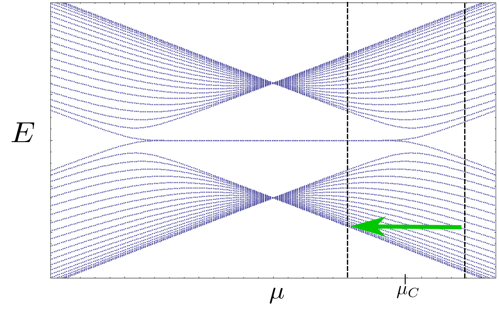
III MBS signatures in MQT
To model the coupled topological and trivial SQUIDs, we start assuming fermionic parity conservation. The wire in a topological phase allows for the introduction of a topological JJ term in addition to the usual Josephson current. The wire is assumed to be much thinner than the SC ring, so that the capacitance and inductance of the device are predominantly defined by the corresponding values from the parent SC and do not depend much on the chemical potential of the wire. We also assume the linear dimensions of the parent SC to be longer than the SC penetration depth in such a way that the SQUID flux “quantization” condition is not changed. Finite-size effects of the ring are not taken into account.
The coupling between the wire and parent SC serves as grounding for the wire and allows for the parity anomaly. The full potential energy thus has and periodic contributions which compete for making (close to) an arbitrary or even-only integer. We consider then a new JJ element to the RCSJ model. The conditions of thin wire guarantee that the phase across the topological JJ is also controlled by the phase across the parent SC junction. The new potential energy of the problem becomes
| (7) | |||||
Here, is a parameter given by the ratio between the critical currents of the parent s-wave junction and the topological one. Its magnitude is roughly controlled by the ratio between the magnitudes of the parent SC gap and the induced p-wave gap in the wire. It will depend on the strength of the proximity effect and on the parent SC 2D density of states. For high chemical potentials, the 1D wire is in a trivial SC phase, whereas for low chemical potentials it enters the topological regime [12].
A subtlety concerns the sign of . It is determined by which parity sector the system is in [12], and, as we assumed the fermionic parity to be conserved, is fixed to a given value along a complete tunneling process.We will come back to this point and address the possibility of fluctuations of this occupancy of the non-local two-level system generated by the MBSs.
Taking all that in consideration, we treat phenomenologically. Assuming that, through gating, we may tune the chemical potential, changes from zero to a saturated value as the chemical potential moves from the trivial to the topological regime. This general behavior is depicted in Fig.3. As the chemical potential goes from smaller to larger values, the Majorana edge modes penetrate the bulk of the wire and, when in the trivial phase, end up coupling and generating a complex fermion which annihilates the topological contribution. In the trivial regime the wire may give a small contribution to the Josephson energy. We neglect these effects assuming that whatever periodic contribution there may be, it is already included in .
This potential also assumes a short junction. In the long junction limit, more bound states develop at the junction and the physics becomes more complicated [8, 9].
Since the wire is much thinner than the s-wave SC and since the p-wave pairing induced in the wire depends on the proximity coupling, it is reasonable to assume that the saturated value of is not very large and we will focus our quantitative discussions on this case. On the other hand, by adding to the the JJ of the parent SC a secondary loop, we may actually control the value of [4], and as such, of , thus allowing for some control on this parameter.
At this point we are ready to discuss qualitatively the consequences of this proposal. We look mainly at two possible signatures, namely, changes in the tunneling rates and shifts in the harmonic oscillator levels. The former might be probed in actual tunneling experiments while the latter may be studied in spectroscopy or coherent tunneling experiments. Fig.4 illustrates the two phenomena and summarizes our main ideas.
One sees how the competition between arbitrary integer and even integer flux takes place. The well becomes shallower while the one is deepened in comparison with the trivial situation (this actually depends on the sign of , whose subtleties will be discussed further ahead, and, for now, we keep in mind that the opposite sign would only bring an opposite scenario).
We may exploit many different schemes to study the consequences of the topological regime. Fig.5 gives some possibilities. In all cases we take a physical value of and shift around the symmetric value for the non-topological regime . For the sake of clearly describing the different situations we take a value of . We note, however, that its actual physical value might be much smaller.
In Figs.5a and 5b we see how situations of enhancing and suppressing the tunneling in the well may be exchanged, just by tilting the potential monitoring from to . These plots also make clear that the suppression or enhancement are actually not symmetric around .
The last two cases of 5c and 5d present very interesting possible applications. In Fig.5c, we see that starting with a symmetric potential, in a Schrödinger’s cat state, we may transform the qubit into a simple classical bit or tune the quantum state into a preferred value of the flux, just as a function of the chemical potential. In Fig.5d we see how to create an adiabatic pump from the unit flux to zero flux and back by lowering the chemical potential into the topological regime and raising it back to the trivial situation.
IV Quantitative results
Now we discuss quantitatively the consequences of our proposals. In order to keep ourselves on safe physical grounds, we use real parameters and units taken from [4]. Namely, we have F, H and keep in mind that experiments are done at temperatures of the order of K. We consider shallow potentials, as tunneling signatures are our main goals. For comparison, we take the same values for the flux bias and parameters when calculating frequencies and tunneling rates. Note however that, if resonance experiments are in mind, deeper wells should be preferred, as many oscillation levels may develop in this case. With all these in mind, we may calculate the frequency and tunneling rate shifts as functions of .
For the frequency we locate numerically the minima of the potential as a function of and evaluate equation (5). In Fig.6 we plot the corresponding results, for both positive and negative values of and for (in red) and (in blue).
The results show that if we have a ratio of about 5% between the Majorana critical current and the parent SQUID critical current, we may achieve a frequency shift of 1 GHz. Different values of shift the curves and, for small , the slopes have small deviations. It should be noted, however, that smaller values of actually also enhance , since this is a ratio of the critical currents.

For the tunneling rate the calculation is slightly more involved. In the non-dissipative limit it may be simply calculated from Callan and Coleman’s instanton calculation scheme [21]. In summary, it resumes to a saddle point approximation in the path integral approach, considering paths in an inverted potential starting and ending at the equilibrium point. The result reduces to
| (8) |
where
| (9) | |||||
| (10) |
and
| (11) |
Here is the classical “bounce” solution in the saddle point approximation and we used the equations of motion and energy conservation to write independently from the exact solution . The prime in the denominator determinant in means that the zero eigenvalue should be omitted. The parameter is the width of the barrier the particle has to tunnel through and is again the small oscillations frequency around the metastable minimum.
Instead of evaluating all the factors from the complicated potential (7), we follow the standard procedure and approximate it by a “quadratic-plus-cubic” potential,
| (12) |
This is a very reasonable approximation [22] and allows us to write the tunneling rate in terms of dimensionless integrals as
| (13) |
The factor is dimensionless by definition and in the non-dissipative limit that we are considering is given by [22, 23].
Considering these, we may calculate numerically the minima and maxima from the original potential, from which we can extract . The results are shown in Fig.7. Again, for different values of , the slopes of the curves change. In particular, again for (5% ratio between critical currents), the tunneling rate presents variations of Hz.

Figures 6 and 7 are our main results. As mentioned before, some care must be taken regarding the depth of the wells, when thinking of tunneling or resonance signatures. Frequencies must always be kept at small values, such that we avoid exciting undesirable quasi-particles in resonance experiments. Also, in tunneling experiments small tunneling rates demand too large coherence times to observe the tunneling. It is remarkable that, nevertheless, the expected signatures manifest themselves in such a way that one can hope to actually measure them.
V Parity fluctuations and robustness
Now we turn to the problem of parity fluctuations. As discussed beforehand, in this section we adopt a more heuristic point of view, discussing the consequences more qualitatively and leaving a proper treatment of the issue for future work. We will show that not only MQT measurements are robust against parity fluctuations, but also that these fluctuations enhance the differences in the tunneling rates.
The issue of fluctuations actually enriches the problem. We must now be careful with the different time scales present, as discussed in Ref.[8]. The first time scale we need to think about is the one which controls the parity fluctuation. The second time scale is the one related to the evolution of the phase difference across the JJ.
Two main sources of fermions are responsible for fluctuations, namely, thermal excitation of quasiparticles or hopping from localized states in the bulk. These mechanisms are exponentially suppressed at low temperatures. In the case when this process happens much faster than the evolution of the SC phase (or the magnetic flux in our case), one has to be careful and consider a proper thermal average of the current [24]. A rigorous way to take this situation into account is to model phenomenologically the parity fluctuation through a Fokker-Planck equation and consider all possible combinations of tunneling processes [15].
We argue that this situation is improbable as follows. As long as the phase is away from , as in the two potential wells of our potential, the different parity branches are far away from each other. The gap separating them is large (of the order of the induced p-wave gap magnitude) and the low temperatures, necessary for the macroscopic quantum behavior of the device to manifest itself, should be enough to suppress fluctuations [15]. In an adiabatic evolution of the phase through , however, the system may access the crossing point and even the lowest temperatures may introduce corrections.
It turns out that quantum tunneling do not describe adiabatic evolutions of the phase. In a thermally activated phase slip, one might describe the time within which the process take place by dividing the total “distance” traveled by the “particle” by its speed. In our case, the situation is mode subtle. Tunneling rates describe the lifetime of a metastable state but the transition itself is much faster. Since the phase/flux behaves quantum mechanically as a “position operator”, defining how long the system spends at a given transition is not necessarily straightforward. The problem of the tunneling time is controversial and has been explored extensively [25]. A characteristic time for this process is given by
| (14) |
where is the imaginary momentum under the barrier,
| (15) |
and is the height of the barrier. In the mechanical picture, this is the same as , where the mass of the particle and the width of the potential barrier. In our case,
| (16) | |||||
| (17) |
but it has been argued that it is not always that this time has physical significance [25].
A safe claim is that, for sure, the time evolution of the phase across the junction is not adiabatic in a tunneling experiment and we focus our attention now onto the picture that parity fluctuations are slower than the tunneling process. In this case, the parity symmetry breaking will allow for the coupling and gapping of the two parity eigenstates. The simple way to model this is to consider the low energy projected Hamiltonian as
where the are the Majorana modes at the wire’s ends, defining a two-level system given by the complex fermions
| (19) |
This Hamiltonian is to be regarded as a mean-level description of the Hamiltonian in [8], which describes inelastic processes responsible for parity flipping events. We just want to study the qualitative features of this system and, as such, capture them into the parameters , which are normalized by . Clearly, for , this Hamiltonian does not conserve the fermionic parity and a gap opens up in the Andreev bound states spectrum as illustrated in Fig.8a.
For non-vanishing , a gap is opened at the two different parity states, restoring the periodicity to the energy levels. The new potential for the SQUID is then given by
| (20) | |||||
In this case, a gap of order opens up in the Andreev states spectrum. This situation actually leads to two consequences. Firstly, lifts the degeneracy of the trivial potential at . This slight raising or lowering of the potential barrier has little consequences for tunneling rates. This can be understood by noticing that the coefficient depends linearly on the frequency and quadratically on . The raising/lowering of the barrier height by mainly affects the frequency, leaving the width intact and generating very small corrections to the tunneling rate.


There is, however, a second important point. Figures 8a and 8b summarizes the situation. The spectrum has no periodicity anymore. One sees, in a closer analysis, that effectively the new potential interpolates between the two parity states, exchanging to opposite parities as crosses . Consider for definiteness that the system is prepared in the positive state. The tunneling barrier width now has become wider and this clearly gives a substantial deviation to the tunneling rate. The opposite would happen if one started from the red curve, with a shrinking of but still a substantial deviation to the tunneling rate from the trivial case would take place. In many realizations one would have to average over the two possibilities.

Clearly, at , if we have an enhancement of the tunneling rate as compared to . This shows that a slow parity fluctuation acts in favor of the tunneling signatures for detecting TSC in rf-SQUIDs. One notices, on the other hand, that the flux pumps described in Fig.5d and the “transmutation” of a qubit into a classical bit from 5c are not possible in this situation.
VI -junction
We now briefly extend the discussion of the previous sections to the case of - junctions. We have been considering the total phase across the junction to be totally controlled by the flux through the loop. Now we assume that the SC also builds a phase across the junction.
The idea follows from the discussion in[26], where the Andreev spectrum of the Kitaev wire is studied thoroughly. This discussion encompasses several cases, including open and closed wires and finite size effects. It is seen that both open and closed limits may be made symmetric under proper conditions, such that the potential becomes sinusoidal.
The flux dynamics is then described by the following potential,
| (21) | |||||
Competition between even and odd minima now is absent. Both wells are lifted or lowered, depending on the parity eigenstate, as illustrated in Fig.10. This is however, different from the parity broken case discussed in the last section, as the topological part of the potential is clearly periodic. Tunneling between different branches in this situation seems to give smaller differences than those in our original case.

Similarly to the parity broken situation, this case is not so interesting as the open wire in the sense that we cannot engineer flux pumps and qubits that may be tuned into simple bits as in the discussion of Fig.5. The typical behavior of the signatures in frequency and tunneling rates are quite remarkable in this case, since they are the opposite from the case of the open wire. As one can see in Fig.11, the roles of positive and negative parity are now inverted.


One might use this in the parity conserving limit to distinguish between the physics of closed or open wire. When parity conservation is broken, the differences between the two cases may disappear.
VII Conclusions
We have studied topological rf-SQUIDs and analyzed the consequences of the topological phase in MQT experiments. The resonance phenomena proposed are expected to give valuable evidence of the existence of the superconducting topological phase. These proposals have the additional advantage of avoiding some of the difficulties that arise in the interpretation of transport experiments.
From a phenomenological model, we show that the crossover between trivial and topological phases may be probed by looking at shifts in the tunneling rates and oscillation frequencies of SQUIDs in the macroscopic quantum regime. The limit of small critical currents ratio is analyzed, although one may hope to have some control over its magnitude. The introduction of a second loop in the parent SC, for example, allows for tuning [4] and, as such, . Moreover, the topological part of the critical current itself depends on the junction length, as well as on the strength of the pairing [2, 8].
Parity breaking is found to work in favor of the detection of the topological phase, as long as the fluctuations are slower than the phase evolution. As we argued, due to the non-adiabatic nature of the flux tunneling process, it is reasonable to expect this to be the general case. This is in accordance with the quantitative results in the limit of fast phase slipping in the context of SC-QSHI-SC biased junctions from[15]. In the latter, the authors also propose to detect the TSC phase in a SC-QSHI-SC junction by addressing the consequences of strong parity fluctuations in thermally activated phase slipping. The authors claim, on the other hand, that in the zero temperature limit, telegraph noise (from parity fluctuation events) averages the voltage across the device to zero at low external currents. Quantum tunneling implies that a drift will actually remain, even in the very low temperature limit, and a finite voltage should develop even for very small bias currents.
The setup in which we described our ideas requires fine tuning of the device to achieve topological superconductivity, as well as means for tuning into and out of the topological phase. For simplicity, we restricted ourselves to a toy model based on the SC coupled to strong SO wire device of [10, 11]. Our ideas, however, do not rely much on the geometry of the device. Corbino geometries like described in Fu and Kane [8] or, as discussed, open SC-QSHI-SC current biased junctions are most likely the proper systems in which this physics should be studied. These junctions are very promising systems for the realization of the TSC phase, among other reasons, for avoiding the necessity of chemical potential fine tuning.
Tuning between phases in these situations is also easily achieved by the application of in-plane magnetic fields. These devices are, however, characterized by larger Majorana contributions to the critical currents as compared to the periodic one, that is, these systems work in the regime of large . In this case, MQT between even integer flux states may be achieved, with small shifts from the expected rates due to the non-topological currents. Parity fluctuations will likely spoil the periodicity of the potential again, restoring the tunneling barrier width to a much smaller value corresponding to non-topological regime.
Acknowledgments
The authors acknowledge fruitful discussions with S. Ryu, T. Hughes and S.-P. Lee. The authors are particularly indebted with and grateful for enlightening discussions with J. C. Y. Teo. This work was supported by FAPESP under grants 2009/18336-0 and 2012/03210-3. VS acknowledges financial support from DOE DE-FG02-07ER46453. AOC is supported by Instituto Nacional de Ciência e Tecnologia de Informação Quântica (INCT-IQ) under grants CNPq - 610020/2009-9 and FAPESP - 2008/57856-6.
References
- [1] C. W. J. Beenakker, Annu. Rev. Con. Mat. 4, 113 (2013).
- [2] J. Alicea, Rep. Prog. Phys. 75, 076501 (2012).
- [3] S. B. Bravyi and A. Y. Kitaev, Ann. of Phys. 298, 210 (2002).
- [4] J. R. Friedman, V. Patel, W. Chen, S. K. Tolpygo, and J. E. Lukens, Nature 406, 43 (2000).
- [5] Y. Makhlin, G. Schön, and A. Shnirman, Rev. Mod. Phys. 73, 357 (2001).
- [6] M. Greiter, X.-G. Wen, and F. Wilczek, Nucl. Phys. B 374, 567 (1992).
- [7] R. L. Willett, L. N. Pfeiffer, and K. W. West, Proceedings of the National Academy of Sciences 106, 8853 (2009) .
- [8] L. Fu and C. L. Kane, Phys. Rev. B 79, 161408 (2009).
- [9] C. W. J. Beenakker, D. I. Pikulin, T. Hyart, H. Schomerus, and J. P. Dahlhaus, Phys. Rev. Lett. 110, 017003 (2013).
- [10] R. M. Lutchyn, J. D. Sau, and S. Das Sarma, Phys. Rev. Lett. 105, 077001 (2010).
- [11] Y. Oreg, G. Refael, and F. von Oppen, Phys. Rev. Lett. 105, 177002 (2010).
- [12] J. Alicea, Y. Oreg, G. Refael, F. von Oppen, and M. P. A. Fisher, Nat Phys 7, 412 (2011).
- [13] A. Kitaev, arXiv:quant-ph/9707021v1 (1997).
- [14] B. van Heck, F. Hassler, A. R. Akhmerov, and C. W. J. Beenakker, Phys. Rev. B 84, 180502 (2011).
- [15] S.-P. Lee, K. Michaeli, J. Alicea, and A. Yacoby, arXiv: 1403.2747v1 (2014) cond-mat 1403.2747v1 .
- [16] K. K. Likharev, Dynamics of Josephson Junctions and Circuits (Gordon and Breach, 1986).
- [17] M. Tinkham, Introduction to Superconductivity (McGraw-Hill, 1996).
- [18] Caldeira, An Introduction to Macroscopic Quantum Phenomena and Quantum Dissipation (Cambridge University Press, 2014).
- [19] A. O. Caldeira and A. J. Leggett, Annals of Physics 149, 374 (1983).
- [20] A. J. Leggett, J. Phys.: Condens. Matter 14, R415 (2002).
- [21] C. G. Callan and S. Coleman, Phys. Rev. D 16, 1762 (1977).
- [22] L.-D. Chang and S. Chakravarty, Phys. Rev. B 29, 130 (1984).
- [23] J. Langer, Annals of Physics 41, 108 (1967).
- [24] H.-J. Kwon, V. M. Yakovenko, and K. Sengupta, Low Temperature Physics 30, 613 (2004).
- [25] R. Landauer and T. Martin, Rev. Mod. Phys. 66, 217 (1994).
- [26] P. Lucignano, F. Tafuri, and A. Tagliacozzo, arXiv e-prints 1302.5242v2 (2013) cond-mat .
- [27] Y. Kim, J. Cano, and C. Nayak, Phys. Rev. B 86, 235429 (2012).
- [28] S. Takei, B. M. Fregoso, V. Galitski, and S. Das Sarma, Phys. Rev. B 87, 014504 (2013).