Bayesian Probabilistic Matrix Factorization: A User Frequency Analysis

[7] considers a constrained version of PMF with an offset on the user feature vectors depending on the movies the user watched. For each movie $k\in\{1,\ldots,M\}$, introduce a $d$ dimensional latent vector $W_{k}$, and modify the expectation of the rating in equation (2.1) as

Where we have defined $n_{i}=\sum_{k^{\prime}=1}^{M}I_{i,k^{\prime}}$ the number of items observed by user $i$, and $S_{i}=\delta_{U}U_{i}+\delta_{W}\sum_{k=1}^{M}I_{i,k}W_{k}/n_{i}$ the combined user / side feature contribution by user $i$.. This ensures the user offset is on the same scale for all users, independent of the number of items observed. Equation (2.4) explicitly includes delta functions $\delta_{U},\delta_{W}\in\{0,1\}$ to emphasize this as an extension to the vanilla PMF model. When $\delta_{W}=0$, the model includes only user-specific latent features in the user offset, reducing to Equation (2.1). If $\delta_{U}=0$, then the model does not consider user features.

To highlight the contribution of this extension, note that users with few or no ratings will have a posterior for $U_{i}$ that is close to the prior. Hence, $U_{i}^{\top}V_{j}$ will be close to the overall average, with the inner product between the $W_{k}$ and $V_{j}$ shifting the rating based on the ratings of other users who also rated the same item.

To make this abstract, constrained PMF introduces a new set of features $W_{k},k=1,\ldots,M$ for each column of the rating matrix $R$. The prediction for the value of entry $(i,u)$ in this matrix is the inner product of the feature associated with the row $U_{i}$ and the feature associated with the column $V_{j}$, plus the inner produce of the column feature $V_{j}$ and the average of these additional feature $W_{k}$ that are associated with observed entries in this row. This abstraction highlights the symmetric nature of these latent side features. The most reliable inference on these additional side features $W_{k}$ will be obtained when they are associated with the dimension of the matrix with less sparsity (row-wise or column-wise).

A similar constraint can be placed on the items by transposing the user-item matrix. The model without side features is invariant to this transposition. For the model with side features, the transposition modifies the expectation of the rating to be

Where we have defined $m_{j}=\sum_{\ell=1}^{N}I_{\ell,j}$ to number of observed ratings for item $j$.

When the side features $W_{k}$ offset the user features $U_{i}$, the contribution from each user to the inner product is affected. Similarly, when the side features $W_{k}$ offset the item features $V_{j}$ as in Equation (2.5), the contribution from each item to the inner product is affected. Since both the user and item features $U_{i},V_{j}$ can be close to the prior from lack of data in the respective rows / columns of the matrix, overall performance will be improved when the side features $W_{k}$ are introduced to shift either the user or item contribution away from the prior.

Learning for PMF is performed by maximizing the log-posterior over the parameters $(U,V,\gamma,\eta)$ given the data

Maximizing this posterior with respect to the parameters is equivalent to minimizing the sum of squared error function with quadratic regularization terms on the parameters:

In practice, we find learning is improved by learning the parameters in stages. In the first stage, we fix the features $U,V$ to zero and learn the biases $\gamma,\eta$ by minimizing

Once estimates for $\gamma_{1:N},\eta_{1:M}$ are obtained, we then learn $U,V$ by minimizing

Batch gradient descent with momentum was used to find an approximate MAP estimate for these parameters. To reduce the number of tuning parameters, a common penalty and learning rate was assumed for all features. The final MAP estimate was selected by stopping gradient descent when error on the validation set increased.

The choice of conjugate prior distributions yields tractable posterior distributions that are easy to sample from. In particular, the user, item and side features are multivariate Gaussian distributions. They are similar to the form derived in [6], with two exceptions. Our derivation includes the scaling from the precision factors $\alpha_{i},\beta_{j}$, and also the shifting effect from the side features $W_{k}$. The posterior for the user features is

The full derivation of these is given in Appendices F, G, and summarized in Tables H.1–H.2 in Appendix H.

The conditional distribution for the feature hyper-parameters is unaffected by the addition of the precision factors and the side features. The symmetry in the probabilistic formulation of the model means the form is identical. The posterior for the user hyper-parameters is

The posterior for the hyper-parameters of the item and side features is analogous.

The precisions have the same Gamma conditional posterior as in [4],

In the case of truncated precisions, Gibbs sampling can still be achieved through the introduction of a latent variable [1].

Samples of the features $(U_{i},V_{j},W_{k})$, the precisions $(\alpha_{i},\beta_{j},\tau)$, the hyper-parameters $(\mu_{U},\Lambda_{U})$, $(\mu_{V},\Lambda_{V})$, $(\mu_{K},\Lambda_{K})$, and the biases $(\gamma_{i},\eta_{j})$ are obtained by running a Markov Chain with stationary distribution equal to the true posterior distribution over the parameters. The Gibbs algorithm is Algorithm 1 in the Appendix.

After iteration $t$, we have samples for the features $(U^{(t)}_{i},V^{(t)}_{j},W^{(t)}_{k})$, the precisions $(\alpha^{(t)}_{i},\beta^{(t)}_{j},\tau^{(t)})$, the hyper-parameters $(\mu^{(t)}_{U},\Lambda^{(t)}_{U})$, $(\mu^{(t)}_{V},\Lambda^{(t)}_{V})$, $(\mu^{(t)}_{K},\Lambda^{(t)}_{K})$, and the biases $(\gamma^{(t)}_{i},\eta^{(t)}_{j})$. We estimate the ratings via:

The prediction after $T$ runs of the Gibbs sampler is the average:

Rather than attempting to make inference on the true posterior distribution $p(\theta\;|\;R)$, Variational methods makes dependence assumptions on the parameters $\theta$, formalizes them as an unknown joint distribution $Q(\theta)$, and infers the distribution and choice of parameters on $Q(\theta)$ to make it a good approximation to $p(\theta\;|\;R)$. There are two decisions to be made: the form of the approximation, and how to measure “close”.

To measure the distance between the approximation $Q$ and the truth $p$, we use Kullback-Leibler (KL) divergence,

The values of $\theta$ are selected to minimize the KL divergence,

The KL divergence in equation (6.6) can be rewritten as

Rearranging, we express the log probability of the data, $\log p(R)$ in terms of two quantities involving the variational distribution: the KL divergence and the entropy $\mathcal{H}(Q)=\mathrm{E}_{Q}[\log p(Q)]$.

Since $\log p(R)$ is fixed, minimizing the KL is equivalent to jointly maximizing the second and third terms, corresponding to the expected complete log likelihood and the entropy. This expression is known as the variational lower bound. We derive this in Appendix I. To make the optimization tractable, a mean field approximation is frequently chosen, where the parameters $\theta$ are independent in the approximation $Q$. This leads to Equation (6.6) factorizing with respect to $\theta$,

Optimization can then be performed sequentially over parameters until convergence is achieved, as measure by the variational lower bound. Optimizing Equation (6.9), or the factorized equivalent in Equation (6.10), with respect to $\theta$ imposes assumptions on the distribution of $\theta$

Our approximation follows the standard structured mean field approximation in the literature [4],

This approximation assumes pairwise independence between the user, item, and side features, while allowing for structure in the latent feature hyper-parameters.

Under this mean field approximation, it can be shown that $Q(\alpha_{i}),Q(\beta_{j}),Q(\tau)$ are Gamma distributions, possibly truncated depending on the model chosen for $p(\theta,R)$ (see Appendix). Inference for the optimal parameters follows immediately as the MAP estimate is still available in a closed form as,

This is just the unbounded MAP estimate, with barriers at the truncation endpoints.

The variational algorithm is described in pseudo-code in Algorithm 2 in the Appendix. The prediction after $T$ full updates of the parameters under the variational algorithm is the prediction given the current variational approximation:

A starting point for the Gibbs sampler and variational algorithm was obtained through a multi-step MAP estimation phase. In the first step, we learned the user and item offsets, $\gamma_{i},\eta_{j}$ through batch gradient descent on the sum-of-squares errors term with prediction $\hat{r}_{i,j}=\gamma_{i}+\eta_{j}$ with quadratic regularizers for the biases,

By learning $\gamma_{i},\eta_{j}$ prior to learning the user and item feature vectors, we ensure that the user and item biases are accounted for in these parameters, and not absorbed as constants in the feature vectors. This is crucial as it prevents singularity issues with the variational algorithm. Learning in this stage is terminated when the training prediction error converges.

With these offsets, we learn the user, item, and side feature vectors using batch gradient descent on the sum-of-squares errors term with quadratic regularizers for the features,

Again, a common penalty and learning rate was assumed for all feature vectors to reduce the number of tuning parameters. 20-dimensional vectors were estimated to facilitate comparison with previous work in the literature [4].

Finally, for the precision models, we set $\alpha_{i},\beta_{j},\tau$ to the maximum likelihood estimates based on the learned user / item parameters

These estimates are coupled, and we iterate through the set of precisions until convergence. Note that learning the precisions after learning the features does not change the actual prediction.

We first consider the performance of the variational algorithm on the model with no side features, no precision factors, and with the default choice of hyper-parameters. Under this setup, the variational lower bound monotonically increases and converges within the first 10 full updates of the parameter set. Despite this, there is overfitting in both the training and test set. The model is unable to improve upon the MAP estimate, see Figure 8.1 (left column).

Further investigation shows that the MAP estimate obtained is probabilistically unlikely under the prior selected, specifically the hyper-parameters of the Gaussian-Wishart priors. The MAP values do not suggest a Wishart scale matrix set to the identity. We rerun variational inference using a modified set of hyper-parameters. Letting $U^{(0)}_{i}$ and $V^{(0)}_{j}$ denote the features obtained in the map estimate, we set

For our map estimate, this creates a scale matrix $W_{0}$ with diagonal elements ranging from $38-82$. We refer to this modified choice of prior as the “MAP-driven” prior.

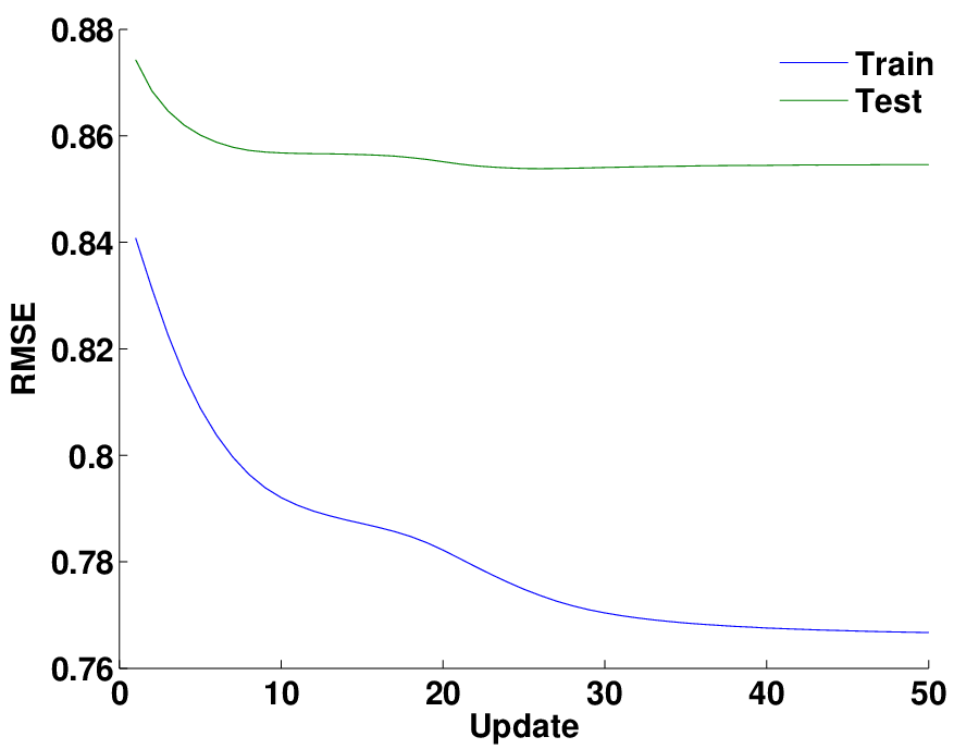
This choice of hyper-parameters allows the variational algorithm to improve on the RMSE obtained by the MAP estimate, but is prone to overfitting on the test set prior to the convergence of the variational lower bound, see Figure 8.1 (middle column). The training lower bound starts to converge after approximately 50 full updates of the variables, while the test error reaches a minimum of 0.8538 after 26 updates. By the time the lower bound has converged, this has increased to 0.8546.

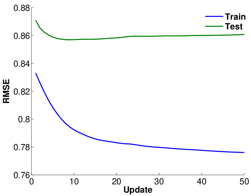
Assessing the convergence of the robust precision model, in practice, is more difficult. The inclusion of user and item multiplicative precision factors allows the variational model to arbitrarily weight the contribution to the complete log-likelihood from different rows and columns in accordance with the predictive accuracy of the model. We discuss this further when we compare the variational algorithm to the Gibbs sampler in Section 8.4. The training lower bound increases almost linearly, with the training error smoothly dropping. The test error reaches a minimum of 0.8570 after nine updates, while the lower bound on the test set continues to decrease for 13 updates, Figure 8.1 (right column). This means that the lower bound on the test set cannot be used to assess convergence, as this happens after overfitting has started.

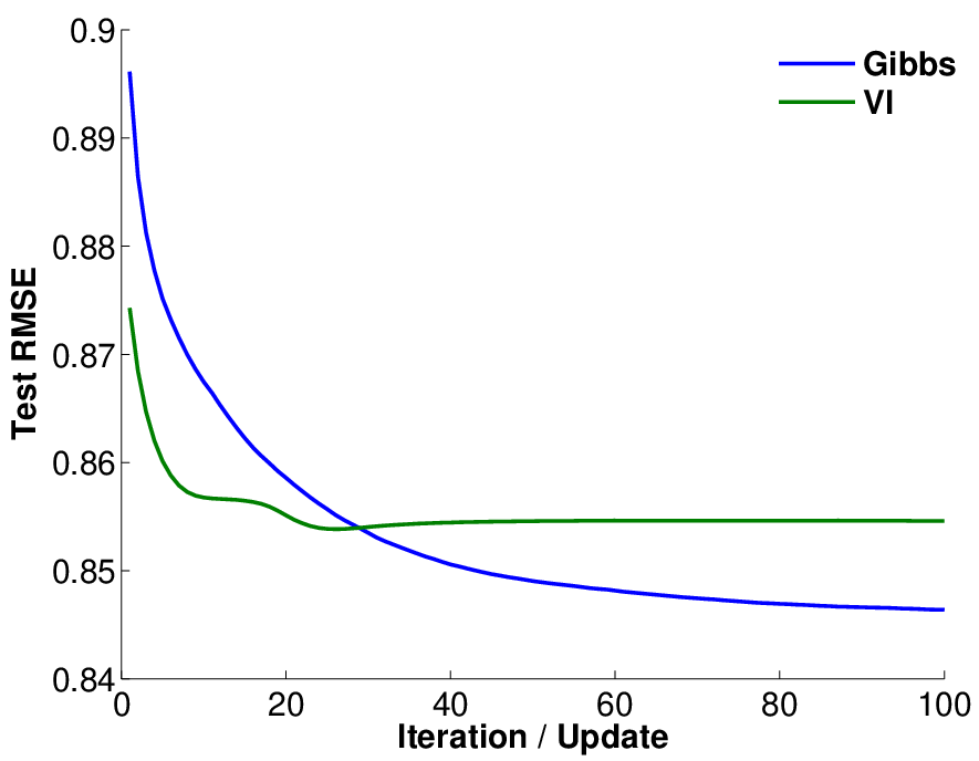
With a fixed choice model (defined by a set of latent features and precision), inference via Gibbs sampling outperforms the Variational mean field approximation. This comparison is trivial when we consider the default choice for the Wishart scale matrix of $W_{0}=\mathbf{I}_{d\times d}$. For a more interesting comparison, we consider the performance of the Gibbs sampler with the default prior and the variational algorithm with the “MAP-driven” prior. For simplicity, we focus our discussion on the basic model without precisions and without side features. We select the Gibbs iteration and Variational update for which the overall test errors are near equal. From Figure 8.2 (a), this is the 29^th update of the parameters under variational inference, and the 29^th iteration of the Gibbs sampler.

With $W_{0}$ driven by the MAP estimate, the variational algorithm outperforms the Gibbs sampler in overall test error for approximately the first 30 iterations. This performance gain is motivated by drops in the first five iterations. After the first five iterations, the variational algorithm experiences diminishing returns. However, the Gibbs sampler continues to drop at a similar rate beyond this point.

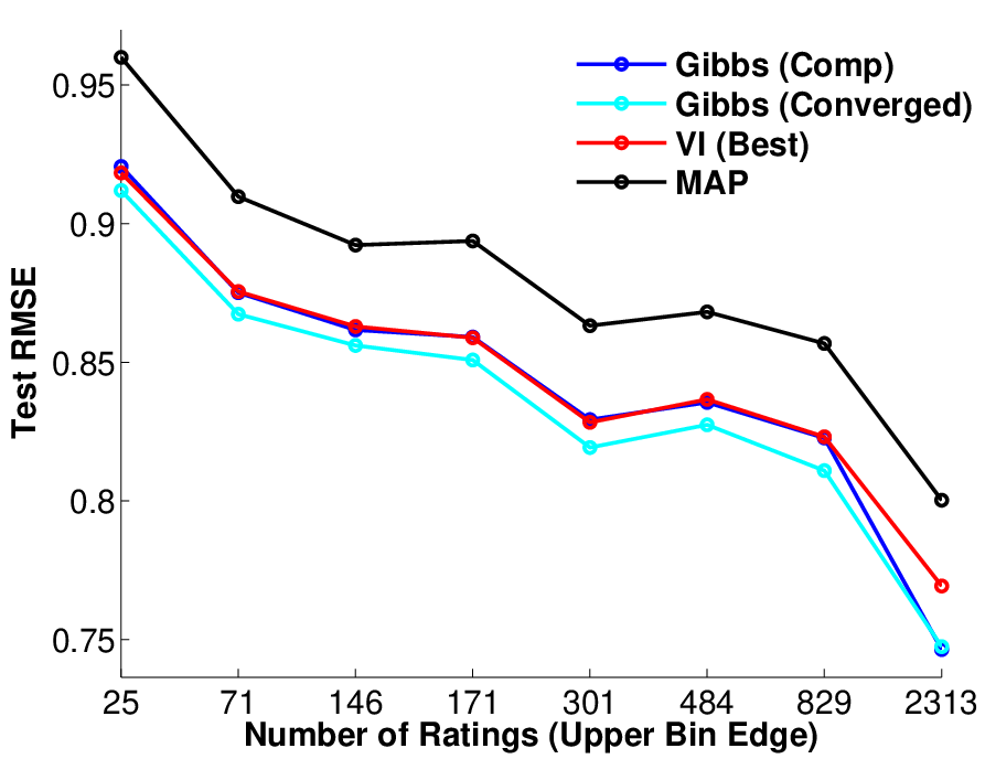
The two algorithms have approximately the same overall error rate on the test set, to within $0.0001$, after the 29th iteration / update. Figure 8.2 (b) illustrates the error of the two inference methods at this point with respect to user frequency. The difference in the performance of the two algorithms is on the order of $0.001$ or less, except for the most frequent bin. This bin corresponds to the $10\%$ most frequent users, and the Gibbs sampler outperforms the variational algorithm.

The performance gap between the Gibbs sampler and the Variational approximation for the most frequent users suggests that the sampling distribution of the user feature vectors has noticeable variability. Figure 8.2 (c) illustrates this by plotting the maximum variance of the $d$-dimensional user feature against the number of ratings the user has in the training set. These are representative values for both inference algorithms after convergence. This space between the plot for the Gibbs sampler and the Variational approximation indicates that the variational approximation tends to produce smaller estimates of the variance than the Gibbs sampler. The vertical line represents users with 829 ratings in the training set, which is the value above which users are included in the last bin in Figure 8.2 (b). The persistent significant difference between these two beyond this point means that there is still variability in the distribution of the user features that the Gibbs sampler is exploiting.

We hope to determine if modelling precisions tends to improve performance for users of a given frequency (cold start, rare, frequent, etc.). To determine this, we examine the final converged error rate on a user frequency basis for a model with and without precisions, holding all else equal. For this comparison, we select the model with side features, and look at the error under Gibbs sampling. The numerical results are in Table 8.2.

While there are some minor departures from equality for moderately frequent users (the third and fourth bin), they are in the fourth decimal place of the error, representing less than a 1% relative change in predictive performance. The largest difference occurs for the most frequent users. This is a relative gain of $0.42\%$. However, these users have predictions that are already well calibrated relative to the rest of the population. Based on these results, we conclude that modelling precisions does not tend to significantly favour users of any given frequency in the test set.

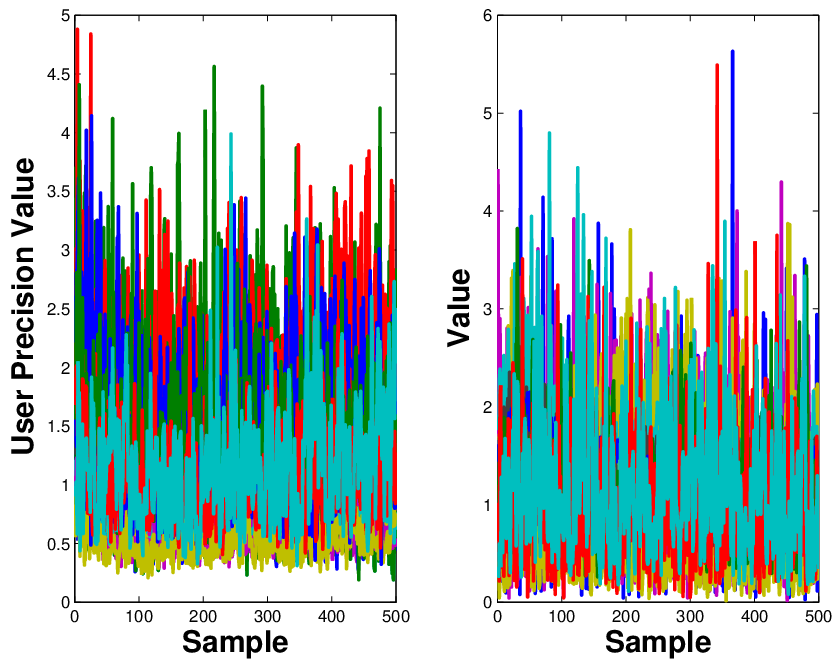
The near equality of both the constant and robust precision models could be a result of a near-constant posterior for the precisions. To check this, we examine traceplots for the user and item precisions, as well as the histogram of the precisions for a sample at convergence. The distribution of both the user and item precisions was clearly non-constant and right skewed. Figure 8.3 (a) displays histograms of the user and item precisions from a Gibbs sampler after convergence, indicating this skewness. Figure 8.3 (b) displays traceplots for a sample of the user and item precisions, showing the sampler mixed well over a range of values. Both of these indicate that the sampler was exploiting the robust precision model. Therefore, the near equality in predictive performance is not a result of model degeneracy.

It has been noted in Section 8.2 that the introduction of precisions prompts the variational algorithm to drive some precisions arbitrarily small and arbitrarily large. The histograms in Figure 8.3 (a) and traceplots in Figure 8.3 (b) indicates that the Gibbs sampler does not suffer from this limitation. For comparison, empirical CDF curves are plotted in Figure 8.3 (c) for the user and item precisions under the variational algorithm (left panel) and the Gibbs sampler (right panel) after convergence. The two panels are similar, though the CDFs for the Variational algorithm have been plotted on a log scale. In other words, the converged values of the precisions under Variational inference are exponentially larger.

It was noted in Section 8.2 that the introduction of precision lead to pathological results with variational inference. We explored if bounding the precisions would alleviate this issue. Using the truncated approach discussed in Section 5, we ran experiments bounding the precisions to values sensible for a scale constrained to the interval $[1,5]$. Some of the initial precision values from the converged values of Equations (8.3) are outside this region. As is appropriate based on our discussion of the MAP estimate for the truncated model, we set such values to the closest boundary point.

We found that bounds of $(1/2,2)$ produced results for MovieLens that outperformed both the constant and robust precision model. These values also delayed the overfitting in the variational approximation for several updates. Overfitting for this model only starts after 20 full updates of the parameters.

Figure 8.4 (a) shows the overall test error of the variational algorithm under the constant, robust, and truncated precision model with the bounds of $(1/2,2)$. These three models have similar behaviour in the initial set of parameter updates. Differences start to appear after the eighth update. At this point, the algorithm overfits on the robust precision model, and continues to drop on the truncated precision model for 3-4 additional iterations. The rate of increase for the two is approximately the same until nearly the 40th parameter update, at which point the truncated precision model tends to increase at a faster rates.

Figure 8.4 (b) shows the test error by user frequency for the algorithm under the two models after 50 full parameter updates. This is the point that the algorithm has begun to overfit in the truncated and the robust model, and has appeared to stabilize for the constant precision model. This graph shows the most significant difference is in the most frequent users. The constant precision model outperforms either heteroskedastic model by a difference of at least 0.1 in test RMSE, a relative improvement in RMSE of $12\%$. The error rates are approximately the same in other user bins, with the constant precision model performing slightly worse for moderately frequent users.

With bounds of the form $(\ell,u)=(1/n,n)$, the truncated model has limiting cases of the constant model as $n\rightarrow 1$ and the robust model as $n\rightarrow\infty$. This leads to the question of how inference on the truncated precision model perform as $n$ changes? Figure 8.4 (c) plots the test error of the variational algorithm for several values of $n$ along with the constant and robust precision model. As expected, larger values of $n$ are similar to the robust precision curve, while smaller values are similar to the constant precision curve. What is surprising is the curve for $n=2$, corresponding to the precision bounds $(1/2,2)$. The variational model obtains a significantly lower error rate under these bounds than the others choices of $n$, or the constant precision model. The consistent tendency for the truncated model to overfit early in learning for larger values of $n$ suggests that the truncation value has little influence on performance after a certain point. However, the improvement for the $n=2$ case over the constant precision model does indicate there is value in allowing for heteroskedastic precision among different users and different items.

The updates for the precision parameters are inversely proportional to the error for that user or item, scaled by the other values of the precisions. In particular, recall that

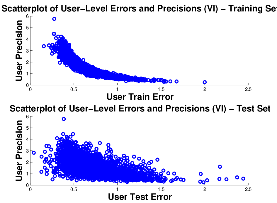
A scatterplot of user precisions versus user training error will show this inverse relationship, similar for items. A good test of generalization is to see if this inverse relationship holds on the test set. Figure 8.5 (a) shows scatterplots of the user and item level errors and precisions for the training (top) and test (bottom) after the third full parameter update. The inverse relationship is clear in the training set, but weak in the test set.

Log transforming Equation (8.5) yields:

Equation (8.6) suggests there should be strong linear correlation between the set of log precisions and log error rates on a user / item level basis for both the training and test set. We compute these for the set of users and items in both the training and test sets, and plot these correlations over iterations in Figure 8.5 (b). The correlations computed on the training set are typically large and stable over iterations. The user correlation is consistently above $0.94$, while the item correlation is consistently above $0.70$. They are not exactly 1 since the updates are sequential, while the correlations are computed after a full parameter update.

When the same values are computed for the user and item errors in the test set, significantly smaller values are obtained, and they decrease monotonically over parameter updates. By the the point the model overfits in the ninth full parameter update, the correlation in the test set for the items has dropped from $0.3440$ to $0.2422$, while the correlation in the test set for the users has dropped from $0.6391$ to $0.5965$. The large difference between the training and test set, both in initial values and in the magnitude of the drop over iterations, shows that the robust model is overfitting and not generalizing to the test set.

We ran similar experiments with truncated precisions with the Gibbs sampler. We did not find that inference with the Gibbs sampler was consistently improved by using truncated precisions. This is not unexpected given that the histograms and traceplots of the precisions in Figure 8.3 (a)-(b) indicate the precisions remain at sensible values under the Gibbs sample.

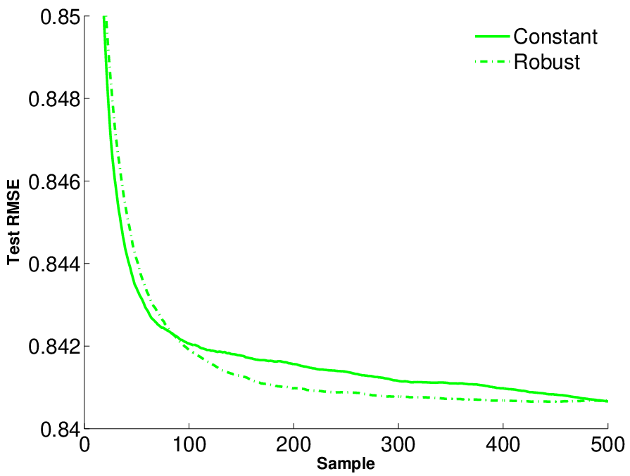
When side features are included in the model, the incremental gain from using a robust precision model is lost, see Table 8.1. The Gibbs sampler converges to the same RMSE value for both the constant and robust precision model.

A closer examination of the test error over iterations show subtle differences in how the common converged value is obtained. In Figure 8.6, we observe the constant model sees a more substantial drop in the first 50 iterations, after which the incremental gain is minor. The robust model takes longer to converge, outperforming the constant model after approximately 80 iterations.

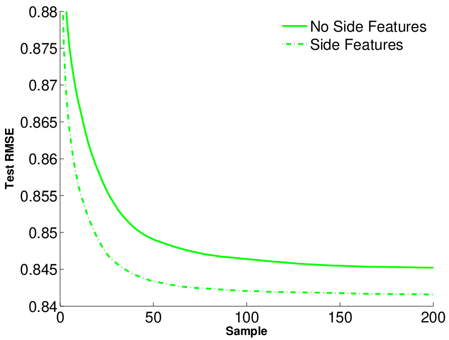
Finally, we consider the effect on predictive gain when including the side features in the model. Table 8.3 tabulates the converged prediction error for the sampler in the model with only user and item features (“No Side”) and the model with user, item, and side features (“Side”) with respect to user frequency. For extremely common users (over 800 ratings), there is no predictive gain. As expected, there is a predictive gain for the least common users (with number or ratings on the order of 20-30). However, it is interesting to note that there is still a noticeable gain in test performance for moderately frequent users, those with several hundred ratings. This gain can be attributed to the side features modelling the correlational influence in the rating structure [3].

Comparing to Table 8.2, we see that the largest relative improvement of $0.42\%$ by the precisions for the top $10\%$ of users is comparable to the gains made by the inclusion of side features for the first five bins, corresponding to half of the MovieLens test set. This highlights the importance of a model to make accurate predictions for rare users. Significant gains overall may be the result of gains for a small selection of users, as is the case for the precision model.

References

• [1] Damien, P. and S. Walker (2001). Sampling truncated normal, beta, and gamma densities. Journal of Computational and Graphical Statistics 10(2), 206–215.
• [2] Fraley, C. and A. E. Raftery (2005). Bayesian Regularization for Normal Mixture Estimation and Model-Based Clustering. Technical Report 486, Department of Statistics.
• [3] Jamali, S. (2013). Probabilistic Models for Recommendation in Social Networks. Ph. D. thesis, Applied Sciences: School of Computing Science.
• [4] Lakshminarayanan, B., G. Bouchard, and C. Archambeau (2011). Robust Bayesian Matrix Factorisation. Journal of Machine Learning Research 15.
• [5] Nadarajah, S. and S. Kotz (2006). R Programs for Computing Truncated Distributions. Journal of Statistical Software 16(Code Snippet 2).
• [6] Salakhutdinov, R. and A. Mnih (2008a). Bayesian probabilistic matrix factorization using Markov chain Monte Carlo. In W. W. Cohen, A. McCallum, and S. T. Roweis (Eds.), ICML, Volume 307 of ACM International Conference Proceeding Series, pp. 880–887. ACM.
• [7] Salakhutdinov, R. and A. Mnih (2008b). Probabilistic Matrix Factorization. In Advances in Neural Information Processing Systems, Volume 20.
Appendix A Appendix
In this section, we provide a series of derivations and ancillary results needed to derive the given results. Primarily, they are needed to obtain the variational lower bound and the conditionals for the variables of interest
Appendix B Algorithms
We provide pseudo-code versions of the Gibbs sampler as Algorithm 1 and the Variational algorithm as Algorithm 2. As discussed previously, the primary difference between the two is with respect the to the feature hyper-parameters. The mean and precision matrix are marginally updated in the Gibbs sampler, but jointly updated in the Variational approximation.
Algorithm 1 Gibbs sampler for Probabilistic Matrix Factorization and the extensions discussed.
for Sample t≥1t\geq 1 do
Sample hyper-parameters
ΛU(t)∼𝒲⁡(ΛU|ν~U,W~U)\Lambda_{U}^{(t)}\sim\mathcal{W}(\Lambda_{U}|\tilde{\nu}_{U},\tilde{W}_{U}) defined by Equation (H.8)
(μU(t)|ΛU(t))∼𝒩⁡(μU|μ~U​β~U​ΛU(t))(\mu_{U}^{(t)}|\Lambda_{U}^{(t)})\sim\mathcal{N}(\mu_{U}|\tilde{\mu}_{U}\tilde{\beta}_{U}\Lambda_{U}^{(t)}) defined by Equation (H.8)
ΛV(t)∼𝒲⁡(ΛV|ν~V,W~V)\Lambda_{V}^{(t)}\sim\mathcal{W}(\Lambda_{V}|\tilde{\nu}_{V},\tilde{W}_{V}) defined analogously to Equation (H.8)
(μV(t)|ΛV(t))∼𝒩⁡(μV|μ~V​β~V​ΛV(t))(\mu_{V}^{(t)}|\Lambda_{V}^{(t)})\sim\mathcal{N}(\mu_{V}|\tilde{\mu}_{V}\tilde{\beta}_{V}\Lambda_{V}^{(t)}) defined analogously to Equation (H.8)
ΛW(t)∼𝒲⁡(ΛW|ν~W,W~W)\Lambda_{W}^{(t)}\sim\mathcal{W}(\Lambda_{W}|\tilde{\nu}_{W},\tilde{W}_{W}) defined analogously to Equation (H.8)
(μW(t)|ΛW(t))∼𝒩⁡(μW|μ~W​β~W​ΛW(t))(\mu_{W}^{(t)}|\Lambda_{W}^{(t)})\sim\mathcal{N}(\mu_{W}|\tilde{\mu}_{W}\tilde{\beta}_{W}\Lambda_{W}^{(t)}) defined analogously to Equation (H.8)
for Each user i=1:Ni=1:N do
Sample user feature Ui(t)∼𝒩⁡(Ui(t)|μUi,ΛUi)U_{i}^{(t)}\sim\mathcal{N}(U_{i}^{(t)}|\mu_{U_{i}},\Lambda_{U_{i}}) defined by Equation (H.1)
Sample user bias γi(t)∼𝒩⁡(γi(t)|μγi,λγi)\gamma_{i}^{(t)}\sim\mathcal{N}(\gamma_{i}^{(t)}|\mu_{\gamma_{i}},\lambda_{\gamma_{i}}) defined by Equation (H.7)
Sample user precision αi(t)∼𝒢⁡(αi(t)|aUi,bUi)\alpha_{i}^{(t)}\sim\mathcal{G}(\alpha_{i}^{(t)}|a_{U_{i}},b_{U_{i}}) defined by Equation (H.4)
end for
for Each item j=1:Mj=1:M do
Sample item feature Vj(t)∼𝒩⁡(Vj(t)|μVj,ΛVj)V_{j}^{(t)}\sim\mathcal{N}(V_{j}^{(t)}|\mu_{V_{j}},\Lambda_{V_{j}}) defined by Equation (H.2)
Sample item bias ηj(t)∼𝒩⁡(ηj(t)|μηj,ληj)\eta_{j}^{(t)}\sim\mathcal{N}(\eta_{j}^{(t)}|\mu_{\eta_{j}},\lambda_{\eta_{j}}) defined analogously to Equation (H.7)
Sample item precision βj(t)∼𝒢⁡(βj(t)|aVj,bVj)\beta_{j}^{(t)}\sim\mathcal{G}(\beta_{j}^{(t)}|a_{V_{j}},b_{V_{j}}) defined analogously to Equation (H.4)
for Each item k=1:Mk=1:M do
Sample side feature Wk(t)∼𝒩⁡(Wk(t)|μWk,ΛWk)W_{k}^{(t)}\sim\mathcal{N}(W_{k}^{(t)}|\mu_{W_{k}},\Lambda_{W_{k}}) defined by Equation (H.3)
Sample global precision τ(t)∼𝒢⁡(τ(t)|aτ,bτ)\tau^{(t)}\sim\mathcal{G}(\tau^{(t)}|a_{\tau},b_{\tau}) defined analogously to Equation (H.4)
Predict test set ratings r^i,j(t)\hat{r}^{(t)}_{i,j} according to Equation (6.4)
Algorithm 2 Variational Algorithm for Probabilistic Matrix Factorization and the extensions discussed.
for Update t≥1t\geq 1 do
Jointly update hyper-parameters
(μU(t),ΛU(t))∼𝒩⁡(μU|μ~U​β~U​ΛU)⋅𝒲⁡(ΛU|ν~U,W~U)(\mu_{U}^{(t)},\Lambda_{U}^{(t)})\sim\mathcal{N}(\mu_{U}|\tilde{\mu}_{U}\tilde{\beta}_{U}\Lambda_{U})\cdot\mathcal{W}(\Lambda_{U}|\tilde{\nu}_{U},\tilde{W}_{U}) defined by Equation (H.8)
(μV(t),ΛV(t))∼𝒩⁡(μV|μ~V​β~V​ΛV)⋅𝒲⁡(ΛV|ν~V,W~V)(\mu_{V}^{(t)},\Lambda_{V}^{(t)})\sim\mathcal{N}(\mu_{V}|\tilde{\mu}_{V}\tilde{\beta}_{V}\Lambda_{V})\cdot\mathcal{W}(\Lambda_{V}|\tilde{\nu}_{V},\tilde{W}_{V}) defined analogously to Equation (H.8)
(μW(t),ΛW(t))∼𝒩⁡(μW|μ~W​β~W​ΛW)⋅𝒲⁡(ΛW|ν~W,W~W)(\mu_{W}^{(t)},\Lambda_{W}^{(t)})\sim\mathcal{N}(\mu_{W}|\tilde{\mu}_{W}\tilde{\beta}_{W}\Lambda_{W})\cdot\mathcal{W}(\Lambda_{W}|\tilde{\nu}_{W},\tilde{W}_{W}) defined analogously to Equation (H.8)
Update user feature Ui(t)∼𝒩⁡(Ui(t)|μUi,ΛUi)U_{i}^{(t)}\sim\mathcal{N}(U_{i}^{(t)}|\mu_{U_{i}},\Lambda_{U_{i}}) defined by Equation (H.1)
Update user bias γi(t)∼𝒩⁡(γi(t)|μγi,λγi)\gamma_{i}^{(t)}\sim\mathcal{N}(\gamma_{i}^{(t)}|\mu_{\gamma_{i}},\lambda_{\gamma_{i}}) defined by Equation (H.7)
Update user precision αi(t)∼𝒢⁡(αi(t)|aUi,bUi)\alpha_{i}^{(t)}\sim\mathcal{G}(\alpha_{i}^{(t)}|a_{U_{i}},b_{U_{i}}) defined by Equation (H.4)
Update item feature Vj(t)∼𝒩⁡(Vj(t)|μVj,ΛVj)V_{j}^{(t)}\sim\mathcal{N}(V_{j}^{(t)}|\mu_{V_{j}},\Lambda_{V_{j}}) defined by Equation (H.2)
Update item bias ηj(t)∼𝒩⁡(ηj(t)|μηj,ληj)\eta_{j}^{(t)}\sim\mathcal{N}(\eta_{j}^{(t)}|\mu_{\eta_{j}},\lambda_{\eta_{j}}) defined analogously to Equation (H.7)
Update item precision βj(t)∼𝒢⁡(βj(t)|aVj,bVj)\beta_{j}^{(t)}\sim\mathcal{G}(\beta_{j}^{(t)}|a_{V_{j}},b_{V_{j}}) defined analogously to Equation (H.4)
Update side feature Wk(t)∼𝒩⁡(Wk(t)|μWk,ΛWk)W_{k}^{(t)}\sim\mathcal{N}(W_{k}^{(t)}|\mu_{W_{k}},\Lambda_{W_{k}}) defined by Equation (H.3)
Update global precision τ(t)∼𝒢⁡(τ(t)|aτ,bτ)\tau^{(t)}\sim\mathcal{G}(\tau^{(t)}|a_{\tau},b_{\tau}) defined analogously to Equation (H.4)
Predict test set ratings r^i,j(t)\hat{r}^{(t)}_{i,j} according to Equation (6.13)
Appendix C Squared Error Term
In the derivation of the conditionals of the feature vectors, it was necessary to expand the squared error term (ri,j−r^i,j)2(r_{i,j}-\hat{r}_{i,j})^{2} and rewrite as constants plus a quadratic in terms of Ui,VjU_{i},V_{j}, and WkW_{k}. We give these three derivations here. For notational convenience, we suppress the bias terms, absorbing both γi\gamma_{i} and ηj\eta_{j} into ri,jr_{i,j}.
C.0.1 Quadratic with Respect to User Features
In terms of the user feature vectors
(ri,j−r^i,j)2\displaystyle(r_{i,j}-\hat{r}_{i,j})^{2} (C.1)
=\displaystyle= [ri,j−(δU​Ui+δWni​∑k=1MIi,k​Wk)⊤​Vj]⊤⋅[ri,j−(δU​Ui+δWni​∑k=1MIi,k​Wk)⊤​Vj]\displaystyle\left[r_{i,j}-\left(\delta_{U}U_{i}+\frac{\delta_{W}}{n_{i}}\sum_{k=1}^{M}I_{i,k}W_{k}\right)^{\top}V_{j}\right]^{\top}\cdot\left[r_{i,j}-\left(\delta_{U}U_{i}+\frac{\delta_{W}}{n_{i}}\sum_{k=1}^{M}I_{i,k}W_{k}\right)^{\top}V_{j}\right]
=\displaystyle= [(ri,j−δWni​∑k=1MIi,k​Wk⊤​Vj)−δU​Ui⊤​Vj]⊤⋅[(ri,j−δWni​∑k=1MIi,k​Wk⊤​Vj)−δU​Ui⊤​Vj]\displaystyle\left[\left(r_{i,j}-\frac{\delta_{W}}{n_{i}}\sum_{k=1}^{M}I_{i,k}W_{k}^{\top}V_{j}\right)-\delta_{U}U_{i}^{\top}V_{j}\right]^{\top}\cdot\left[\left(r_{i,j}-\frac{\delta_{W}}{n_{i}}\sum_{k=1}^{M}I_{i,k}W_{k}^{\top}V_{j}\right)-\delta_{U}U_{i}^{\top}V_{j}\right]
=\displaystyle= [(ri,j−δWni​∑k=1MIi,k​Wk⊤​Vj)⊤−δU​Vj⊤​Ui]⋅[(ri,j−δWni​∑k=1MIi,k​Wk⊤​Vj)−δU​Ui⊤​Vj]\displaystyle\left[\left(r_{i,j}-\frac{\delta_{W}}{n_{i}}\sum_{k=1}^{M}I_{i,k}W_{k}^{\top}V_{j}\right)^{\top}-\delta_{U}V_{j}^{\top}U_{i}\right]\cdot\left[\left(r_{i,j}-\frac{\delta_{W}}{n_{i}}\sum_{k=1}^{M}I_{i,k}W_{k}^{\top}V_{j}\right)-\delta_{U}U_{i}^{\top}V_{j}\right]
=\displaystyle= (ri,j−δWni​∑k=1MIi,k​Wk⊤​Vj)⊤​(ri,j−δWni​∑k=1MIi,k​Wk⊤​Vj)\displaystyle\left(r_{i,j}-\frac{\delta_{W}}{n_{i}}\sum_{k=1}^{M}I_{i,k}W_{k}^{\top}V_{j}\right)^{\top}\left(r_{i,j}-\frac{\delta_{W}}{n_{i}}\sum_{k=1}^{M}I_{i,k}W_{k}^{\top}V_{j}\right)
−2​δU​(ri,j−δWni​∑k=1MIi,k​Wk⊤​Vj)⊤​Vj⊤​Ui+δU2​Ui⊤​Vj​Vj⊤​Ui\displaystyle-2\delta_{U}\left(r_{i,j}-\frac{\delta_{W}}{n_{i}}\sum_{k=1}^{M}I_{i,k}W_{k}^{\top}V_{j}\right)^{\top}V_{j}^{\top}U_{i}+\delta_{U}^{2}U_{i}^{\top}V_{j}V_{j}^{\top}U_{i}
Where the last line follows as Vj⊤​Ui​Ui⊤​Vj=Ui⊤​Vj​Vj⊤​UiV_{j}^{\top}U_{i}U_{i}^{\top}V_{j}=U_{i}^{\top}V_{j}V_{j}^{\top}U_{i}.
C.0.2 Quadratic with Respect to Item Features
In terms of the item feature vectors
(ri,j−r^i,j)2\displaystyle(r_{i,j}-\hat{r}_{i,j})^{2} (C.2)
=\displaystyle= ri,j2−2​ri,j​(δU​Ui+δWni​∑k=1MIi,k​Wk)⊤​Vj\displaystyle r_{i,j}^{2}-2r_{i,j}\left(\delta_{U}U_{i}+\frac{\delta_{W}}{n_{i}}\sum_{k=1}^{M}I_{i,k}W_{k}\right)^{\top}V_{j}
+Vj⊤​(δU​Ui+δWni​∑k=1MIi,k​Wk)​(δU​Ui+δWni​∑k=1MIi,k​Wk)⊤​Vj\displaystyle+V_{j}^{\top}\left(\delta_{U}U_{i}+\frac{\delta_{W}}{n_{i}}\sum_{k=1}^{M}I_{i,k}W_{k}\right)\left(\delta_{U}U_{i}+\frac{\delta_{W}}{n_{i}}\sum_{k=1}^{M}I_{i,k}W_{k}\right)^{\top}V_{j}
C.0.3 Quadratic with Respect to Side Features
Finally, in terms of the side feature vector WkW_{k}, we have
(ri,j−r^i,j)2\displaystyle(r_{i,j}-\hat{r}_{i,j})^{2} (C.3)
=\displaystyle= [(ri,j−(δU​Ui+δWni​∑k≠mIi,k​Wk)⊤​Vj)−δWni​Ii,m​Wm⊤​Vj]⊤\displaystyle\left[\left(r_{i,j}-\left(\delta_{U}U_{i}+\frac{\delta_{W}}{n_{i}}\sum_{k\neq m}I_{i,k}W_{k}\right)^{\top}V_{j}\right)-\frac{\delta_{W}}{n_{i}}I_{i,m}W_{m}^{\top}V_{j}\right]^{\top}
⋅[(ri,j−(δU​Ui+δWni​∑k≠mIi,k​Wk)⊤​Vj)−δWni​Ii,m​Wm⊤​Vj]\displaystyle\cdot\left[\left(r_{i,j}-\left(\delta_{U}U_{i}+\frac{\delta_{W}}{n_{i}}\sum_{k\neq m}I_{i,k}W_{k}\right)^{\top}V_{j}\right)-\frac{\delta_{W}}{n_{i}}I_{i,m}W_{m}^{\top}V_{j}\right]
Let r^i,j,−Wm=(δU​Ui+δWni​∑k≠mIi,k​Wk)⊤​Vj\hat{r}_{i,j,-W_{m}}=\left(\delta_{U}U_{i}+\frac{\delta_{W}}{n_{i}}\sum_{k\neq m}I_{i,k}W_{k}\right)^{\top}V_{j} denote the prediction made without WmW_{m}. Then,
(ri,j−r^i,j)2\displaystyle(r_{i,j}-\hat{r}_{i,j})^{2} (C.4)
=\displaystyle= [(ri,j−r^i,j,−Wm)−δWni​Ii,m​Wm⊤​Vj]⊤⋅[(ri,j−r^i,j,−Wm)−δWni​Ii,m​Wm⊤​Vj]\displaystyle\left[\left(r_{i,j}-\hat{r}_{i,j,-W_{m}}\right)-\frac{\delta_{W}}{n_{i}}I_{i,m}W_{m}^{\top}V_{j}\right]^{\top}\cdot\left[\left(r_{i,j}-\hat{r}_{i,j,-W_{m}}\right)-\frac{\delta_{W}}{n_{i}}I_{i,m}W_{m}^{\top}V_{j}\right]
=\displaystyle= (ri,j−r^i,j,−Wm)⊤​(ri,j−r^i,j,−Wm)−2​δWni​Ii,m​(ri,j−r^i,j,−Wm)​Vj⊤​Wm\displaystyle\left(r_{i,j}-\hat{r}_{i,j,-W_{m}}\right)^{\top}\left(r_{i,j}-\hat{r}_{i,j,-W_{m}}\right)-2\frac{\delta_{W}}{n_{i}}I_{i,m}\left(r_{i,j}-\hat{r}_{i,j,-W_{m}}\right)V_{j}^{\top}W_{m}
+δW2ni2​Wm⊤​Vj​Vj⊤​Wm\displaystyle+\frac{\delta_{W}^{2}}{n_{i}^{2}}W_{m}^{\top}V_{j}V_{j}^{\top}W_{m}
Appendix D Expectation of Forms
D.1 Expectation of Quadratic Forms
Let xx be a random vector with mean μ\mu and covariance matrix Σ\Sigma, and let Λ\Lambda be a symmetric matrix. Then
E⁡[x⊤​Λ​x]=\displaystyle\mathrm{E}[x^{\top}\Lambda x]= tr⁡(Λ​Σ)+μ⊤​Λ​μ\displaystyle\mathrm{tr}\left(\Lambda\Sigma\right)+\mu^{\top}\Lambda\mu (D.1)
Combined with iterated expectation, this is used to find some expectations in the variational lower bound. An alternative is to expand the quadratic, which we give an example of below using the user feature quadratic form.
D.2 User Quadratic Form
In computing the variational lower bound, we need to consider the expectation of quadratic forms such as
EQ​[(Ui−μU)⊤​ΛU​(Ui−μU)]\displaystyle\mathrm{E}_{Q}[(U_{i}-\mu_{U})^{\top}\Lambda_{U}(U_{i}-\mu_{U})] (D.2)
=\displaystyle= EQ​[Ui⊤​ΛU​Ui]−2​EQ​[Ui⊤​ΛU​μu]+EQ​[μU⊤​ΛU​μU]\displaystyle\mathrm{E}_{Q}[U_{i}^{\top}\Lambda_{U}U_{i}]-2\mathrm{E}_{Q}[U_{i}^{\top}\Lambda_{U}\mu_{u}]+\mathrm{E}_{Q}[\mu_{U}^{\top}\Lambda_{U}\mu_{U}]
Which appear from the prior placed on the user, item, and side features. We compute the expectation term by term.
For the first term
EQ​[Ui⊤​ΛU​Ui]=\displaystyle\mathrm{E}_{Q}[U_{i}^{\top}\Lambda_{U}U_{i}]= EQ​[EQ​[Ui⊤​ΛU​Ui|ΛU]]\displaystyle\mathrm{E}_{Q}[\mathrm{E}_{Q}[U_{i}^{\top}\Lambda_{U}U_{i}|\Lambda_{U}]]
=\displaystyle= EQ​[tr⁡(ΛU​ΛUi−1)+μUi⊤​ΛU​μUi]\displaystyle\mathrm{E}_{Q}[\mathrm{tr}\left(\Lambda_{U}\Lambda_{U_{i}}^{-1}\right)+\mu_{U_{i}}^{\top}\Lambda_{U}\mu_{U_{i}}]
=\displaystyle= tr⁡(EQ​[ΛU]​ΛUi−1)+μUi⊤​EQ​[ΛU]​μUi\displaystyle\mathrm{tr}\left(\mathrm{E}_{Q}[\Lambda_{U}]\Lambda_{U_{i}}^{-1}\right)+\mu_{U_{i}}^{\top}\mathrm{E}_{Q}[\Lambda_{U}]\mu_{U_{i}}
=\displaystyle= ν~U​tr​(W~U​ΛUi−1)+ν~U​μUi⊤​W~U​μUi\displaystyle\tilde{\nu}_{U}\mathrm{tr}\left(\tilde{W}_{U}\Lambda_{U_{i}}^{-1}\right)+\tilde{\nu}_{U}\mu_{U_{i}}^{\top}\tilde{W}_{U}\mu_{U_{i}}
For the second term
EQ​[Ui⊤​ΛU​μU]=\displaystyle\mathrm{E}_{Q}[U_{i}^{\top}\Lambda_{U}\mu_{U}]= EQ[EQ[Ui⊤ΛUμU|ΛU,μU]]\displaystyle\mathrm{E}_{Q}[\mathrm{E}_{Q}[U_{i}^{\top}\Lambda_{U}\mu_{U}|\Lambda_{U},\mu_{U}]]
=\displaystyle= EQ​[EQ​[Ui]⊤​ΛU​μU]\displaystyle\mathrm{E}_{Q}[\mathrm{E}_{Q}[U_{i}]^{\top}\Lambda_{U}\mu_{U}]
=\displaystyle= μUi⊤​EQ​[EQ​[ΛU​μU|ΛU]]\displaystyle\mu_{U_{i}}^{\top}\mathrm{E}_{Q}[\mathrm{E}_{Q}[\Lambda_{U}\mu_{U}|\Lambda_{U}]]
=\displaystyle= μUi⊤​EQ​[ΛU]​μ~U\displaystyle\mu_{U_{i}}^{\top}\mathrm{E}_{Q}[\Lambda_{U}]\tilde{\mu}_{U}
=\displaystyle= ν~U​μUi⊤​W~U​μ~U\displaystyle\tilde{\nu}_{U}\mu_{U_{i}}^{\top}\tilde{W}_{U}\tilde{\mu}_{U}
For the final term,
EQ​[μU⊤​ΛU​μU]\displaystyle\mathrm{E}_{Q}[\mu_{U}^{\top}\Lambda_{U}\mu_{U}]
=\displaystyle= EQ[EQ[μU⊤ΛUμU]|ΛU]]\displaystyle\mathrm{E}_{Q}[\mathrm{E}_{Q}[\mu_{U}^{\top}\Lambda_{U}\mu_{U}]|\Lambda_{U}]]
=\displaystyle= EQ​[tr⁡(ΛU​Λ~U−1)+μ~U⊤​ΛU​μ~U]\displaystyle\mathrm{E}_{Q}[\mathrm{tr}\left(\Lambda_{U}\tilde{\Lambda}_{U}^{-1}\right)+\tilde{\mu}_{U}^{\top}\Lambda_{U}\tilde{\mu}_{U}]
=\displaystyle= tr⁡(EQ​[ΛU]​Λ~U−1)+μ~U⊤​EQ​[ΛU]​μ~U\displaystyle\mathrm{tr}\left(\mathrm{E}_{Q}[\Lambda_{U}]\tilde{\Lambda}_{U}^{-1}\right)+\tilde{\mu}_{U}^{\top}\mathrm{E}_{Q}[\Lambda_{U}]\tilde{\mu}_{U}
=\displaystyle= ν~U​tr​(W~U​Λ~U−1)+ν~U​μ~U⊤​W~U​μ~U\displaystyle\tilde{\nu}_{U}\mathrm{tr}\left(\tilde{W}_{U}\tilde{\Lambda}_{U}^{-1}\right)+\tilde{\nu}_{U}\tilde{\mu}_{U}^{\top}\tilde{W}_{U}\tilde{\mu}_{U}
Together, the three terms give,
EQ​[(Ui−μU)⊤​ΛU​(Ui−μU)]\displaystyle\mathrm{E}_{Q}[(U_{i}-\mu_{U})^{\top}\Lambda_{U}(U_{i}-\mu_{U})] (D.3)
−2​ν~U​μUi⊤​W~U​μ~U\displaystyle-2\tilde{\nu}_{U}\mu_{U_{i}}^{\top}\tilde{W}_{U}\tilde{\mu}_{U}
+ν~U​tr​(W~U​Λ~U−1)+ν~U​μ~U⊤​W~U​μ~U\displaystyle+\tilde{\nu}_{U}\mathrm{tr}\left(\tilde{W}_{U}\tilde{\Lambda}_{U}^{-1}\right)+\tilde{\nu}_{U}\tilde{\mu}_{U}^{\top}\tilde{W}_{U}\tilde{\mu}_{U}
=\displaystyle= ν~U​[(μUi−μ~U)⊤​W~U​(μUi−μ~U)+tr⁡(W~U​(ΛUi−1+Λ~U−1))]\displaystyle\tilde{\nu}_{U}\left[(\mu_{U_{i}}-\tilde{\mu}_{U})^{\top}\tilde{W}_{U}(\mu_{U_{i}}-\tilde{\mu}_{U})+\mathrm{tr}\left(\tilde{W}_{U}(\Lambda_{U_{i}}^{-1}+\tilde{\Lambda}_{U}^{-1})\right)\right]
Similar expressions hold for the items and the side features.
D.3 Gamma Random Variable Expectation
If X∼𝒢⁡(α,β)X\sim\mathcal{G}(\alpha,\beta), with probability density function fX​(x|α,β)∝xα−1​e−β​xf_{X}(x|\alpha,\beta)\propto x^{\alpha-1}e^{-\beta x}.
E⁡[log⁡X]=\displaystyle\mathrm{E}[\log X]= −log⁡(β)+ψ⁡(α)\displaystyle-\log(\beta)+\psi(\alpha)
Where ψ⁡(⋅)=dd⋅​log⁡Γ​(⋅)\psi(\cdot)=\frac{d}{d\cdot}\log\Gamma(\cdot). This result important in computing the contribution to the variational lower bound from the user, item, and global precisions.
D.4 Wishart Random Variable Expectation
If 𝐗∼𝒲⁡(n,𝐕)\mathbf{X}\sim\mathcal{W}(n,\mathbf{V}), with probability density function f𝐗(𝐗|n,𝐕)∝|𝐗|(n−p−1)/2e−tr(𝐕−1𝐗)/2f_{\mathbf{X}}(\mathbf{X}|n,\mathbf{V})\propto|\mathbf{X}|^{(n-p-1)/2}e^{-\mathrm{tr}\left(\mathbf{V}^{-1}\mathbf{X}\right)/2}
E⁡[log⁡|X|]=\displaystyle\mathrm{E}[\log|X|]= ∑i=1pψ⁡(n+1−i2)+2​log⁡2+log⁡|𝐕|\displaystyle\sum_{i=1}^{p}\psi\left(\frac{n+1-i}{2}\right)+2\log 2+\log|\mathbf{V}|
Like the last result, this is necessary to compute the variational lower bound, as it appears from the conjugate Normal-Wishart priors.
Appendix E Constrained PMF
In this section, we derive the conditional distribution of the features given the observed rating data with the presence of side information. The inclusion of side information into the model shifts the mean of the user features, and is also re-derived. The conditional for the item features follows by substituting the combination of user and side features for the user features in the original derivation from [6].
For notational convenience, we suppress the offsets, absorbing γi\gamma_{i} and ηj\eta_{j} into ri,jr_{i,j}.
E.1 Conditional Posterior for Side Feature
The inclusion of the the side information WmW_{m} complicates the log likelihood contribution to the log posterior. The square in the exponent of the Gaussian for ri,jr_{i,j} becomes:
log⁡p⁡(ri,j|⋯)=\displaystyle\log p(r_{i,j}|\cdots)= ∑i=1N∑j=1M−Ii,j​αi​βj​τ2[ri,j−(δUUi+δW1ni∑k=1mIi,kWk)⊤Vj]⊤\displaystyle\sum_{i=1}^{N}\sum_{j=1}^{M}-\frac{I_{i,j}\alpha_{i}\beta_{j}\tau}{2}[r_{i,j}-(\delta_{U}U_{i}+\delta_{W}\frac{1}{n_{i}}\sum_{k=1}^{m}I_{i,k}W_{k})^{\top}V_{j}]^{\top} (E.1)
×[ri,j−(δU​Ui+δW​1ni​∑k=1mIi,k​Wk)⊤​Vj],\displaystyle\times[r_{i,j}-(\delta_{U}U_{i}+\delta_{W}\frac{1}{n_{i}}\sum_{k=1}^{m}I_{i,k}W_{k})^{\top}V_{j}],
Where ni=∑k=1MIi,kn_{i}=\sum_{k=1}^{M}I_{i,k}. Using the properties of the transpose and expanding the square yields
∑i=1N∑j=1M−Ii,j​αi​βj​τ2[ri,j−Vj⊤(δUUi+δW1ni∑k=1mIi,kWk)]\displaystyle\sum_{i=1}^{N}\sum_{j=1}^{M}-\frac{I_{i,j}\alpha_{i}\beta_{j}\tau}{2}[r_{i,j}-V_{j}^{\top}(\delta_{U}U_{i}+\delta_{W}\frac{1}{n_{i}}\sum_{k=1}^{m}I_{i,k}W_{k})] (E.2)
×[ri,j−(δU​Ui+δW​1ni​∑k=1mIi,k​Wk)⊤​Vj]\displaystyle\times[r_{i,j}-(\delta_{U}U_{i}+\delta_{W}\frac{1}{n_{i}}\sum_{k=1}^{m}I_{i,k}W_{k})^{\top}V_{j}]
=\displaystyle= ∑i=1N∑j=1M−Ii,j​αi​βj​τ2[ri,j2−2ri,jVj⊤(δUUi+δW1ni∑k=1mIi,kWk)\displaystyle\sum_{i=1}^{N}\sum_{j=1}^{M}-\frac{I_{i,j}\alpha_{i}\beta_{j}\tau}{2}[r_{i,j}^{2}-2r_{i,j}V_{j}^{\top}(\delta_{U}U_{i}+\delta_{W}\frac{1}{n_{i}}\sum_{k=1}^{m}I_{i,k}W_{k})
+Vj⊤(δUUi+δWni∑k=1mIi,kWk)(δUUi+δWni∑k=1mIi,kWk)⊤Vj]\displaystyle+V_{j}^{\top}(\delta_{U}U_{i}+\frac{\delta_{W}}{n_{i}}\sum_{k=1}^{m}I_{i,k}W_{k})(\delta_{U}U_{i}+\frac{\delta_{W}}{n_{i}}\sum_{k=1}^{m}I_{i,k}W_{k})^{\top}V_{j}]
Expanding the quadratic in the final term and dropping terms independent of WmW_{m}, we obtain,
∑i=1N∑j=1M−Ii,j​αi​βj​τ2[−2ri,jVj⊤δWIi,mniWm+2δUδWVj⊤(UiIi,mniWm⊤)Vj\displaystyle\sum_{i=1}^{N}\sum_{j=1}^{M}-\frac{I_{i,j}\alpha_{i}\beta_{j}\tau}{2}[-2r_{i,j}V_{j}^{\top}\delta_{W}\frac{I_{i,m}}{n_{i}}W_{m}+2\delta_{U}\delta_{W}V_{j}^{\top}(U_{i}\frac{I_{i,m}}{n_{i}}W_{m}^{\top})V_{j} (E.3)
OPEN+δW2​Vj⊤​(Ii,m​Wmni+∑k≠mIi,k​Wkni)​(Ii,m​Wmni+∑k≠mIi,k​Wkni)⊤)​Vj\displaystyle+\delta_{W}^{2}V_{j}^{\top}(\frac{I_{i,m}W_{m}}{n_{i}}+\frac{\sum_{k\neq m}I_{i,k}W_{k}}{n_{i}})(\frac{I_{i,m}W_{m}}{n_{i}}+\frac{\sum_{k\neq m}I_{i,k}W_{k}}{n_{i}})^{\top})V_{j}
Note the sum over WkW_{k} has been separated into the term involving WmW_{m} and the sum over the other Wk,k≠mW_{k},k\neq m.
Rearranging vectors to place it in the form μw⊤​Λw​Wm\mu_{w}^{\top}\Lambda_{w}W_{m},
∑i=1N∑j=1M−Ii,j​αi​βj​τ2[−2δWri,jVj⊤Ii,mniWm+2δUδWUi⊤(VjVj⊤)Ii,mniWm\displaystyle\sum_{i=1}^{N}\sum_{j=1}^{M}-\frac{I_{i,j}\alpha_{i}\beta_{j}\tau}{2}[-2\delta_{W}r_{i,j}V_{j}^{\top}\frac{I_{i,m}}{n_{i}}W_{m}+2\delta_{U}\delta_{W}U_{i}^{\top}(V_{j}V_{j}^{\top})\frac{I_{i,m}}{n_{i}}W_{m} (E.4)
+δW2​Wm⊤​(Ii,mni)2​Vj​Vj⊤​Wm+2​δW2​Ii,mni​(∑k≠mIi,k​Wkni)⊤​Vj​Vj⊤​Wm\displaystyle+\delta_{W}^{2}W_{m}^{\top}(\frac{I_{i,m}}{n_{i}})^{2}V_{j}V_{j}^{\top}W_{m}+2\delta_{W}^{2}\frac{I_{i,m}}{n_{i}}(\frac{\sum_{k\neq m}I_{i,k}W_{k}}{n_{i}})^{\top}V_{j}V_{j}^{\top}W_{m}
Adding the log prior (Wm−μw)⊤​Λw​(Wm−μw)/2(W_{m}-\mu_{w})^{\top}\Lambda_{w}(W_{m}-\mu_{w})/2 and grouping terms linear in WmW_{m} and quadratic in WmW_{m}, we obtain the system
ΛWm=\displaystyle\Lambda_{W_{m}}= Λw+δW2​τ​∑i=1N∑j=1MIi,j​Ii,m​αi​βjni2​Vj​Vj⊤\displaystyle\Lambda_{w}+\delta_{W}^{2}\tau\sum_{i=1}^{N}\sum_{j=1}^{M}\frac{I_{i,j}I_{i,m}\alpha_{i}\beta_{j}}{n_{i}^{2}}V_{j}V_{j}^{\top} (E.5)
μWm=\displaystyle\mu_{W_{m}}= ΛWm−1[Λwμw\displaystyle\Lambda_{W_{m}}^{-1}\bigg[\Lambda_{w}\mu_{w}
+τ∑i=1N∑j=1MIi,jαiβj(ri,jVjδWIi,mni−δUδW(VjVj⊤)UiIi,mni\displaystyle+\tau\sum_{i=1}^{N}\sum_{j=1}^{M}I_{i,j}\alpha_{i}\beta_{j}\bigg(r_{i,j}V_{j}\delta_{W}\frac{I_{i,m}}{n_{i}}-\delta_{U}\delta_{W}(V_{j}V_{j}^{\top})U_{i}\frac{I_{i,m}}{n_{i}}
−δW2VjVj⊤Ii,mni2(∑k≠mIi,kWk))]\displaystyle-\delta_{W}^{2}V_{j}V_{j}^{\top}\frac{I_{i,m}}{n_{i}^{2}}(\sum_{k\neq m}I_{i,k}W_{k})\bigg)\bigg]
Rewriting,
μWm=\displaystyle\mu_{W_{m}}= ΛWm−1[Λwμw+(1−u)τ∑(i,j):Ii,j​Ii,m=1αi​βjniVj((ri,j−δUVj⊤Ui)−δWVj⊤∑k≠mIi,k​Wkni)]\displaystyle\Lambda_{W_{m}}^{-1}\bigg[\Lambda_{w}\mu_{w}+(1-u)\tau\sum_{\begin{subarray}{c}(i,j):\\ I_{i,j}I_{i,m}=1\end{subarray}}\frac{\alpha_{i}\beta_{j}}{n_{i}}V_{j}\bigg((r_{i,j}-\delta_{U}V_{j}^{\top}U_{i})-\delta_{W}V_{j}^{\top}\frac{\sum_{k\neq m}I_{i,k}W_{k}}{n_{i}}\bigg)\bigg] (E.6)
This can be re-expressed in a more compact form by defining the prediction made without WmW_{m} as
r^i,j,−Wm=(δU​Ui+δWni​∑k≠mIi,k​Wk)⊤​Vj\displaystyle\hat{r}_{i,j,-W_{m}}=\left(\delta_{U}U_{i}+\frac{\delta_{W}}{n_{i}}\sum_{k\neq m}I_{i,k}W_{k}\right)^{\top}V_{j}
μWm=\displaystyle\mu_{W_{m}}= ΛWm−1[Λwμw+δWτ∑(i,j):Ii,j​Ii,m=1αi​βjniVj(ri,j−r^i,j,−Wm))]\displaystyle\Lambda_{W_{m}}^{-1}\left[\Lambda_{w}\mu_{w}+\delta_{W}\tau\sum_{\begin{subarray}{c}(i,j):\\ I_{i,j}I_{i,m}=1\end{subarray}}\frac{\alpha_{i}\beta_{j}}{n_{i}}V_{j}\left(r_{i,j}-\hat{r}_{i,j,-W_{m}}\right))\right] (E.7)
Which can be interpreted as the inner product between the jthj^{\text{th}} feature vector and the error made by all feature vectors with the mthm^{\text{th}} side feature omitted.
E.2 Conditional Posterior for User Feature
With the inclusion of side features WkW_{k}, the log posterior for UiU_{i} becomes
log⁡p⁡(Ui|⋯)=\displaystyle\log p(U_{i}|\cdots)= τ​αi2​∑j=1MIi,j​βj​(ri,j−r^i,j)2+(Ui−μU)​ΛU​(Ui−μU)\displaystyle\frac{\tau\alpha_{i}}{2}\sum_{j=1}^{M}I_{i,j}\beta_{j}(r_{i,j}-\hat{r}_{i,j})^{2}+(U_{i}-\mu_{U})\Lambda_{U}(U_{i}-\mu_{U}) (E.8)
Expanding the squared term yields,
(ri,j−r^i,j)2\displaystyle(r_{i,j}-\hat{r}_{i,j})^{2} (E.9)
−2​u​(ri,j−δWni​∑k=1MIi,k​Wk⊤​Vj)⊤​Vj⊤​Ui+δU2​Ui⊤​Vj​Vj⊤​Ui\displaystyle-2u\left(r_{i,j}-\frac{\delta_{W}}{n_{i}}\sum_{k=1}^{M}I_{i,k}W_{k}^{\top}V_{j}\right)^{\top}V_{j}^{\top}U_{i}+\delta_{U}^{2}U_{i}^{\top}V_{j}V_{j}^{\top}U_{i}
Plugging into equation E.8 and dropping terms not involving UiU_{i} yields,
log⁡p⁡(Ui|⋯)=\displaystyle\log p(U_{i}|\cdots)= τ​αi2​∑j=1MIi,j​βj​[−2​u​(ri,j−δWni​∑k=1MIi,k​Wk⊤​Vj)⊤​Vj⊤​Ui+δU2​Ui⊤​Vj​Vj⊤​Ui]\displaystyle\frac{\tau\alpha_{i}}{2}\sum_{j=1}^{M}I_{i,j}\beta_{j}\left[-2u\left(r_{i,j}-\frac{\delta_{W}}{n_{i}}\sum_{k=1}^{M}I_{i,k}W_{k}^{\top}V_{j}\right)^{\top}V_{j}^{\top}U_{i}+\delta_{U}^{2}U_{i}^{\top}V_{j}V_{j}^{\top}U_{i}\right] (E.10)
+(Ui−μU)​ΛU​(Ui−μU)\displaystyle+(U_{i}-\mu_{U})\Lambda_{U}(U_{i}-\mu_{U})
Which shows that the conditional posterior for UiU_{i} is Gaussian with parameters
ΛUi=\displaystyle\Lambda_{U_{i}}= ΛU+δU​τ​αi​∑j=1MIi,j​βj​Vj​Vj⊤\displaystyle\Lambda_{U}+\delta_{U}\tau\alpha_{i}\sum_{j=1}^{M}I_{i,j}\beta_{j}V_{j}V_{j}^{\top} (E.11)
μUi=\displaystyle\mu_{U_{i}}= ΛUi−1​[ΛU​μU+δU​τ​αi​∑j=1MIi,j​βj​Vj​(ri,j−δW​Vj⊤​(∑k=1MIi,k​Wkni))]\displaystyle\Lambda_{U_{i}}^{-1}\left[\Lambda_{U}\mu_{U}+\delta_{U}\tau\alpha_{i}\sum_{j=1}^{M}I_{i,j}\beta_{j}V_{j}\left(r_{i,j}-\delta_{W}V_{j}^{\top}\left(\frac{\sum_{k=1}^{M}I_{i,k}W_{k}}{n_{i}}\right)\right)\right]
Note that the inclusion of side information affects only the mean, not the precision.
Appendix F Optimal Variational Distributions
In this section, we derive the optimal variational distribution under the mean field approximation of equation (6.11). The subsections are as follows:
• •
In Subsection F.1, we derive the optimal variational distribution for the user features;
In Subsection F.3, we derive the optimal variational distribution for the item features;
In Subsection F.4, we derive the optimal variational distribution for the side features;
In Subsection F.5, we derive the optimal variational distribution for the user, item, and global precisions;
In Subsection F.6, we derive the optimal variational distribution for the user hyper-parameters. By symmetry, the results for item and side hyper-parameters follow immediately.
F.1 User Feature Vectors
For the user feature vectors, the terms involving UiU_{i} are the conditional expectation for the rating ri,jr_{i,j} and the prior for the feature vector UiU_{i}. We then have
∑j=1MIi,jlogp(ri,j|Ui,Vj,W1:m,αi,βj,τ)+logp(Ui|μU,ΛU)\displaystyle\sum_{j=1}^{M}I_{i,j}\log p(r_{i,j}|U_{i},V_{j},W_{1:m},\alpha_{i},\beta_{j},\tau)+\log p(U_{i}|\mu_{U},\Lambda_{U}) (F.1)
=\displaystyle= −Ii,j2ταi∑j=1Mβj(ri,j−r^i,j)2+12log|ΛU|−12(Ui−μU)⊤ΛU(Ui−μU)\displaystyle-\frac{I_{i,j}}{2}\tau\alpha_{i}\sum_{j=1}^{M}\beta_{j}(r_{i,j}-\hat{r}_{i,j})^{2}+\frac{1}{2}\log|\Lambda_{U}|-\frac{1}{2}(U_{i}-\mu_{U})^{\top}\Lambda_{U}(U_{i}-\mu_{U})
=\displaystyle= −Ii,j2ταi∑j=1Mβj(−2δU(ri,j−δWni∑k=1MIi,kWk⊤Vj)Vj⊤Ui+δUUi⊤VjVj⊤Ui)\displaystyle-\frac{I_{i,j}}{2}\tau\alpha_{i}\sum_{j=1}^{M}\beta_{j}\left(-2\delta_{U}\left(r_{i,j}-\frac{\delta_{W}}{n_{i}}\sum_{k=1}^{M}I_{i,k}W_{k}^{\top}V_{j}\right)V_{j}^{\top}U_{i}+\delta_{U}U_{i}^{\top}V_{j}V_{j}^{\top}U_{i}\right)
−12​(Ui−μU)⊤​ΛU​(Ui−μU)\displaystyle-\frac{1}{2}(U_{i}-\mu_{U})^{\top}\Lambda_{U}(U_{i}-\mu_{U})
Which shows the variational distribution for UiU_{i} is Gaussian, with parameters
μUi=\displaystyle\mu_{U_{i}}= ΛUi−1​[ΛU​μU+δU​τ​αi​∑j=1MIi,j​βj​Vj​(ri,j−δW​Vj⊤​(∑k=1MIi,k​Wkni))]\displaystyle\Lambda_{U_{i}}^{-1}\left[\Lambda_{U}\mu_{U}+\delta_{U}\tau\alpha_{i}\sum_{j=1}^{M}I_{i,j}\beta_{j}V_{j}\left(r_{i,j}-\delta_{W}V_{j}^{\top}\left(\frac{\sum_{k=1}^{M}I_{i,k}W_{k}}{n_{i}}\right)\right)\right] (F.2)
ΛUi=\displaystyle\Lambda_{U_{i}}= ΛU+δU​τ​αi​∑j=1MIi,j​βj​Vj​Vj⊤\displaystyle\Lambda_{U}+\delta_{U}\tau\alpha_{i}\sum_{j=1}^{M}I_{i,j}\beta_{j}V_{j}V_{j}^{\top}
F.2 User Offset
If we include a user offset γi\gamma_{i}, then the relevant terms are
\displaystyle ∑j=1MIi,j​log⁡p⁡(ri,j|⋯)+log⁡p⁡(γi|μγ,λγ)\displaystyle\sum_{j=1}^{M}I_{i,j}\log p(r_{i,j}|\cdots)+\log p(\gamma_{i}|\mu_{\gamma},\lambda_{\gamma}) (F.3)
∑j=1MIi,j2​log⁡|ΛU|−Ii,j2​τ​αi​∑j=1M(ri,j−r^i,j)2+12​log⁡λγ−λγ2​(γi−μγ)2\displaystyle\sum_{j=1}^{M}\frac{I_{i,j}}{2}\log|\Lambda_{U}|-\frac{I_{i,j}}{2}\tau\alpha_{i}\sum_{j=1}^{M}(r_{i,j}-\hat{r}_{i,j})^{2}+\frac{1}{2}\log\lambda_{\gamma}-\frac{\lambda_{\gamma}}{2}(\gamma_{i}-\mu_{\gamma})^{2}
The quadratic (ri,j−r^i,j)2(r_{i,j}-\hat{r}_{i,j})^{2} can be rewritten as
(ri,j−r^i,j)2=\displaystyle(r_{i,j}-\hat{r}_{i,j})^{2}= (ri,j−γi−ηj−Si⊤​Vj)2\displaystyle(r_{i,j}-\gamma_{i}-\eta_{j}-S_{i}^{\top}V_{j})^{2}
=\displaystyle= γi2−2​γi​(ri,j−ηj−Si⊤​Vj)+(ri,j−ηj−Si⊤​Vj)2\displaystyle\gamma_{i}^{2}-2\gamma_{i}(r_{i,j}-\eta_{j}-S_{i}^{\top}V_{j})+(r_{i,j}-\eta_{j}-S_{i}^{\top}V_{j})^{2}
Inserting into Equation F.3, taking expectations, and retaining terms involving γi\gamma_{i} only, we get that the optimal distribution for γi\gamma_{i} is univariate Gaussian, with parameters
λ~γi=\displaystyle\tilde{\lambda}_{\gamma_{i}}= τ​αi​∑j=1MIi,j​βj+λγ\displaystyle\tau\alpha_{i}\sum_{j=1}^{M}I_{i,j}\beta_{j}+\lambda_{\gamma} (F.4)
μ~γi=\displaystyle\tilde{\mu}_{\gamma_{i}}= λ~γi−1​(λγ​μγ+τ​αi​∑j=1MIi,j​βj​(ri,j−ηj−Si⊤​Vj))\displaystyle\tilde{\lambda}_{\gamma_{i}}^{-1}\left(\lambda_{\gamma}\mu_{\gamma}+\tau\alpha_{i}\sum_{j=1}^{M}I_{i,j}\beta_{j}(r_{i,j}-\eta_{j}-S_{i}^{\top}V_{j})\right)
F.3 Item Feature Vectors
By symmetry, the terms involving VjV_{j} are
∑i=1NIi,jlogp(ri,j|Ui,Vj,W1:m,αi,βj,τ)+logp(Vj|μV,ΛV)\displaystyle\sum_{i=1}^{N}I_{i,j}\log p(r_{i,j}|U_{i},V_{j},W_{1:m},\alpha_{i},\beta_{j},\tau)+\log p(V_{j}|\mu_{V},\Lambda_{V}) (F.5)
=\displaystyle= −Ii,j2βjτ∑i=1Nαi(ri,j−r^i,j)2+12log|ΛV|−12(Vj−μV)⊤ΛV(Vj−μV)\displaystyle-\frac{I_{i,j}}{2}\beta_{j}\tau\sum_{i=1}^{N}\alpha_{i}(r_{i,j}-\hat{r}_{i,j})^{2}+\frac{1}{2}\log|\Lambda_{V}|-\frac{1}{2}(V_{j}-\mu_{V})^{\top}\Lambda_{V}(V_{j}-\mu_{V})
=\displaystyle= −Ii,j2βjτ∑i=1Nαi(−2ri,j(δUUi+δWni∑k=1MIi,kWk)⊤Vj)\displaystyle-\frac{I_{i,j}}{2}\beta_{j}\tau\sum_{i=1}^{N}\alpha_{i}\left(-2r_{i,j}\left(\delta_{U}U_{i}+\frac{\delta_{W}}{n_{i}}\sum_{k=1}^{M}I_{i,k}W_{k}\right)^{\top}V_{j}\right)
−12​(Vj−μV)⊤​ΛV​(Vj−μV)\displaystyle-\frac{1}{2}(V_{j}-\mu_{V})^{\top}\Lambda_{V}(V_{j}-\mu_{V})
Which shows the variational distribution for VjV_{j} is Gaussian, with parameters
μVj=\displaystyle\mu_{V_{j}}= ΛVj−1​[ΛV​μV+τ​βj​∑i=1NIi,j​αi​(ri,j−(δU​Ui+δWni​∑k=1MIi,k​Wk)⊤​Vj)]\displaystyle\Lambda_{V_{j}}^{-1}\left[\Lambda_{V}\mu_{V}+\tau\beta_{j}\sum_{i=1}^{N}I_{i,j}\alpha_{i}(r_{i,j}-(\delta_{U}U_{i}+\frac{\delta_{W}}{n_{i}}\sum_{k=1}^{M}I_{i,k}W_{k})^{\top}V_{j})\right] (F.6)
ΛVj=\displaystyle\Lambda_{V_{j}}= ΛV+τ​βj​∑i=1NIi,j​αi​(δU​Ui+δWni​∑k=1MIi,k​Wk)​(δU​Ui+δWni​∑k=1MIi,k​Wk)⊤\displaystyle\Lambda_{V}+\tau\beta_{j}\sum_{i=1}^{N}I_{i,j}\alpha_{i}(\delta_{U}U_{i}+\frac{\delta_{W}}{n_{i}}\sum_{k=1}^{M}I_{i,k}W_{k})(\delta_{U}U_{i}+\frac{\delta_{W}}{n_{i}}\sum_{k=1}^{M}I_{i,k}W_{k})^{\top}
F.4 Side Feature Vectors
The terms involving WmW_{m} are
∑i=1N∑j=1MIi,jlogp(ri,j|Ui,Vj,W1:m,αi,βj,τ)+logp(Wm|μW,ΛW)\displaystyle\sum_{i=1}^{N}\sum_{j=1}^{M}I_{i,j}\log p(r_{i,j}|U_{i},V_{j},W_{1:m},\alpha_{i},\beta_{j},\tau)+\log p(W_{m}|\mu_{W},\Lambda_{W}) (F.7)
=\displaystyle= τ2​∑i=1N∑j=1MIi,j​αi​βj​(ri,j−r^i,j)2−12​(Wm−μW)⊤​ΛW​(Wm−μW)\displaystyle\frac{\tau}{2}\sum_{i=1}^{N}\sum_{j=1}^{M}I_{i,j}\alpha_{i}\beta_{j}(r_{i,j}-\hat{r}_{i,j})^{2}-\frac{1}{2}(W_{m}-\mu_{W})^{\top}\Lambda_{W}(W_{m}-\mu_{W})
=\displaystyle= −τ2∑i=1N∑j=1MIi,jαiβj(−2δWniIi,m(ri,j−r^i,j,−Wm)Vj⊤Wm+δWni2Wm⊤VjVj⊤Wm)\displaystyle-\frac{\tau}{2}\sum_{i=1}^{N}\sum_{j=1}^{M}I_{i,j}\alpha_{i}\beta_{j}\left(-2\frac{\delta_{W}}{n_{i}}I_{i,m}(r_{i,j}-\hat{r}_{i,j,-W_{m}})V_{j}^{\top}W_{m}+\frac{\delta_{W}}{n_{i}^{2}}W_{m}^{\top}V_{j}V_{j}^{\top}W_{m}\right)
−12​(Wm−μW)⊤​ΛW​(Wm−μW)\displaystyle-\frac{1}{2}(W_{m}-\mu_{W})^{\top}\Lambda_{W}(W_{m}-\mu_{W})
Where r^i,j,−Wm=(δU​Ui+δWni​∑k≠mIi,k​Wk)⊤​Vj\hat{r}_{i,j,-W_{m}}=\left(\delta_{U}U_{i}+\frac{\delta_{W}}{n_{i}}\sum_{k\neq m}I_{i,k}W_{k}\right)^{\top}V_{j} denotes the prediction made without WmW_{m}. This shows the variational distribution for WmW_{m} is Gaussian with parameters
μWm=\displaystyle\mu_{W_{m}}= ΛWm−1[Λwμw+δWτ∑(i,j):Ii,j​Ii,m=1αi​βjniVj(ri,j−r^i,j,−Wm)]\displaystyle\Lambda_{W_{m}}^{-1}\left[\Lambda_{w}\mu_{w}+\delta_{W}\tau\sum_{\begin{subarray}{c}(i,j):\\ I_{i,j}I_{i,m}=1\end{subarray}}\frac{\alpha_{i}\beta_{j}}{n_{i}}V_{j}\left(r_{i,j}-\hat{r}_{i,j,-W_{m}}\right)\right] (F.8)
ΛWm=\displaystyle\Lambda_{W_{m}}= ΛW+δWτ∑(i,j):Ii,j​Ii,m=1αi​βjni2VjVj⊤\displaystyle\Lambda_{W}+\delta_{W}\tau\sum_{\begin{subarray}{c}(i,j):\\ I_{i,j}I_{i,m}=1\end{subarray}}\frac{\alpha_{i}\beta_{j}}{n_{i}^{2}}V_{j}V_{j}^{\top}
Note the product of the two indicators Ii,j​Ii,mI_{i,j}I_{i,m}. The side information sum only considers those users who rated this item, and then considers those items these users rated.
F.5 Precisions
The terms involving αi\alpha_{i} are
∑j=1MIi,jlogp(ri,j|Ui,Vj,W1:m,αi,βj,τ)+logp(αi|aU,bU)\displaystyle\sum_{j=1}^{M}I_{i,j}\log p(r_{i,j}|U_{i},V_{j},W_{1:m},\alpha_{i},\beta_{j},\tau)+\log p(\alpha_{i}|a_{U},b_{U}) (F.9)
=\displaystyle= ∑j=1MIi,j2​log⁡αi−τ2​∑j=1MIi,j​βj​(ri,j−r^i,j)2+(aU−1)​log⁡αi−bU​αi\displaystyle\sum_{j=1}^{M}\frac{I_{i,j}}{2}\log\alpha_{i}-\frac{\tau}{2}\sum_{j=1}^{M}I_{i,j}\beta_{j}(r_{i,j}-\hat{r}_{i,j})^{2}+(a_{U}-1)\log\alpha_{i}-b_{U}\alpha_{i}
Which shows the variational distribution for αi\alpha_{i} is Gamma, with parameters
a~Ui=\displaystyle\tilde{a}_{U_{i}}= aU+12​∑j=1MIi,j\displaystyle a_{U}+\frac{1}{2}\sum_{j=1}^{M}I_{i,j} (F.10)
b~Ui=\displaystyle\tilde{b}_{U_{i}}= bU+τ2​∑j=1MIi,j​βj​(ri,j−r^i,j)2\displaystyle b_{U}+\frac{\tau}{2}\sum_{j=1}^{M}I_{i,j}\beta_{j}(r_{i,j}-\hat{r}_{i,j})^{2}
Identical derivations show the variational distributions for βj\beta_{j} and τ\tau are Gamma, with parameters
a~Vj=\displaystyle\tilde{a}_{V_{j}}= aV+12​∑i=1NIi,j\displaystyle a_{V}+\frac{1}{2}\sum_{i=1}^{N}I_{i,j} (F.11)
b~Vj=\displaystyle\tilde{b}_{V_{j}}= bV+τ2​∑i=1NIi,j​αi​(ri,j−r^i,j)2\displaystyle b_{V}+\frac{\tau}{2}\sum_{i=1}^{N}I_{i,j}\alpha_{i}(r_{i,j}-\hat{r}_{i,j})^{2}
a~τ=\displaystyle\tilde{a}_{\tau}= aτ+12​∑i=1N∑j=1MIi,j\displaystyle a_{\tau}+\frac{1}{2}\sum_{i=1}^{N}\sum_{j=1}^{M}I_{i,j}
b~τ=\displaystyle\tilde{b}_{\tau}= bτ+12​∑i=1N∑j=1MIi,j​αi​βj​(ri,j−r^i,j)2\displaystyle b_{\tau}+\frac{1}{2}\sum_{i=1}^{N}\sum_{j=1}^{M}I_{i,j}\alpha_{i}\beta_{j}(r_{i,j}-\hat{r}_{i,j})^{2}
F.6 User / Item / Side Feature Hyper-parameters
The terms involving the user hyper-parameters μU,ΛU\mu_{U},\Lambda_{U} are
∑i=1Nlog⁡p⁡(Ui|μU,ΛU)+log⁡p⁡(μU|μ0,β0​ΛU)+log⁡(ΛU|ν0,W0)\displaystyle\sum_{i=1}^{N}\log p(U_{i}|\mu_{U},\Lambda_{U})+\log p(\mu_{U}|\mu_{0},\beta_{0}\Lambda_{U})+\log(\Lambda_{U}|\nu_{0},W_{0}) (F.12)
=\displaystyle= N2​log⁡|ΛU|−12​∑i=1N(Ui−μU)⊤​ΛU​(Ui−μU)\displaystyle\frac{N}{2}\log|\Lambda_{U}|-\frac{1}{2}\sum_{i=1}^{N}(U_{i}-\mu_{U})^{\top}\Lambda_{U}(U_{i}-\mu_{U})
+12​log⁡ΛU−β02​(μU−μ0)⊤​ΛU​(μU−μ0)\displaystyle+\frac{1}{2}\log\Lambda_{U}-\frac{\beta_{0}}{2}(\mu_{U}-\mu_{0})^{\top}\Lambda_{U}(\mu_{U}-\mu_{0})
+ν0−d−12​log⁡|ΛU|−12​tr​(W0−1​ΛU)\displaystyle+\frac{\nu_{0}-d-1}{2}\log|\Lambda_{U}|-\frac{1}{2}\mathrm{tr}\left(W_{0}^{-1}\Lambda_{U}\right)
Using derivations involving the completion of the square, see ex: [2], the quadratic terms can be rearranged as
∑i=1N(Ui−μU)⊤​ΛU​(Ui−μU)+β0​(μU−μ0)⊤​ΛU​(μU−μ0)\displaystyle\sum_{i=1}^{N}(U_{i}-\mu_{U})^{\top}\Lambda_{U}(U_{i}-\mu_{U})+\beta_{0}(\mu_{U}-\mu_{0})^{\top}\Lambda_{U}(\mu_{U}-\mu_{0}) (F.13)
=\displaystyle= tr⁡([∑i=1N(Ui−μU)​(Ui−μU)⊤+β0​(μU−μ0)​(μU−μ0)⊤]​ΛU)\displaystyle\mathrm{tr}\left(\left[\sum_{i=1}^{N}(U_{i}-\mu_{U})(U_{i}-\mu_{U})^{\top}+\beta_{0}(\mu_{U}-\mu_{0})(\mu_{U}-\mu_{0})^{\top}\right]\Lambda_{U}\right)
=\displaystyle= tr⁡([N⁡(U¯−μU)​(U¯−μU)⊤+∑i=1N(Ui−U¯)​(Ui−U¯)⊤+β0​(μU−μ0)​(μU−μ0)]​ΛU)\displaystyle\mathrm{tr}\left(\left[N(\overline{U}-\mu_{U})(\overline{U}-\mu_{U})^{\top}+\sum_{i=1}^{N}(U_{i}-\overline{U})(U_{i}-\overline{U})^{\top}+\beta_{0}(\mu_{U}-\mu_{0})(\mu_{U}-\mu_{0})\right]\Lambda_{U}\right)
=\displaystyle= tr⁡([(N+β0)​(μU−μ~U)​(μU−μ~U)⊤+N​β0N+β0​(U¯−μ0)​(U¯−μ0)⊤+∑i=1N(Ui−U¯)​(Ui−U¯)⊤]​ΛU)\displaystyle\mathrm{tr}\left(\left[(N+\beta_{0})(\mu_{U}-\tilde{\mu}_{U})(\mu_{U}-\tilde{\mu}_{U})^{\top}+\frac{N\beta_{0}}{N+\beta_{0}}(\overline{U}-\mu_{0})(\overline{U}-\mu_{0})^{\top}+\sum_{i=1}^{N}(U_{i}-\overline{U})(U_{i}-\overline{U})^{\top}\right]\Lambda_{U}\right)
Where we have defined
μ~U=\displaystyle\tilde{\mu}_{U}= N​U¯+β0​μ0N+β0\displaystyle\frac{N\overline{U}+\beta_{0}\mu_{0}}{N+\beta_{0}} (F.14)
We can now write the μU,ΛU\mu_{U},\Lambda_{U} terms as
∑i=1Nlog⁡p⁡(Ui|μU,ΛU)+log⁡p⁡(μU|μ0,β0​ΛU)+log⁡(ΛU|ν0,W0)\displaystyle\sum_{i=1}^{N}\log p(U_{i}|\mu_{U},\Lambda_{U})+\log p(\mu_{U}|\mu_{0},\beta_{0}\Lambda_{U})+\log(\Lambda_{U}|\nu_{0},W_{0}) (F.15)
=\displaystyle= 12​log⁡|ΛU|−12​(μU−μ~U)⊤​[(N+β0)​ΛU]​(μU−μ~U)\displaystyle\frac{1}{2}\log|\Lambda_{U}|-\frac{1}{2}(\mu_{U}-\tilde{\mu}_{U})^{\top}[(N+\beta_{0})\Lambda_{U}](\mu_{U}-\tilde{\mu}_{U})
+N+ν0−d−12​log⁡|ΛU|\displaystyle+\frac{N+\nu_{0}-d-1}{2}\log|\Lambda_{U}|
−12​tr​(W0−1+[N​β0N+β0​(U¯−μ0)​(U¯−μ0)⊤+∑i=1N(Ui−U¯)​(Ui−U¯)⊤]​ΛU)\displaystyle-\frac{1}{2}\mathrm{tr}\left(W_{0}^{-1}+\left[\frac{N\beta_{0}}{N+\beta_{0}}(\overline{U}-\mu_{0})(\overline{U}-\mu_{0})^{\top}+\sum_{i=1}^{N}(U_{i}-\overline{U})(U_{i}-\overline{U})^{\top}\right]\Lambda_{U}\right)
Which shows the variational distribution for (μU,ΛU)(\mu_{U},\Lambda_{U}) is a Normal-Wishart with parameters
μ~U=\displaystyle\tilde{\mu}_{U}= N​U¯+β0​μ0N+β0\displaystyle\frac{N\overline{U}+\beta_{0}\mu_{0}}{N+\beta_{0}} (F.16)
Λ~U=\displaystyle\tilde{\Lambda}_{U}= (N+β0)​ΛU\displaystyle(N+\beta_{0})\Lambda_{U}
ν~U=\displaystyle\tilde{\nu}_{U}= N+ν0\displaystyle N+\nu_{0}
W~U−1=\displaystyle\tilde{W}_{U}^{-1}= W0−1+N​β0N+β0​(U¯−μ0)​(U¯−μ0)⊤+∑i=1N(Ui−U¯)​(Ui−U¯)⊤\displaystyle W_{0}^{-1}+\frac{N\beta_{0}}{N+\beta_{0}}(\overline{U}-\mu_{0})(\overline{U}-\mu_{0})^{\top}+\sum_{i=1}^{N}(U_{i}-\overline{U})(U_{i}-\overline{U})^{\top}
Analogous statements (with the appropriate sample size, feature averages, etc.) hold for the item and side feature vectors.
Appendix G Gibbs Distributions
Many of the conditional posteriors for all the parameters of interest match those derived for variational inference by the independence assumptions. The exception is for the feature hyper-parameters, as the variational approximation was a joint distribution over these. Here, we derive the conditional posterior for the user feature hyper-parameters. The others follow by symmetry.
The log posterior distribution for (μU,ΛU)(\mu_{U},\Lambda_{U}) has been shown to the take the form of a Gaussian Wishart Distribution, with parameters given in Equation F.16. The conditional for ΛU\Lambda_{U} takes the form
log⁡p⁡(ΛU|μU,⋯)=\displaystyle\log p(\Lambda_{U}|\mu_{U},\cdots)= +12​log⁡|ΛU|+ν~U−d−12​log|ΛU|−12​tr​(W~U−1​ΛU)\displaystyle+\frac{1}{2}\log|\Lambda_{U}|+\frac{\tilde{\nu}_{U}-d-1}{2}\log|\Lambda_{U}|-\frac{1}{2}\mathrm{tr}\left(\tilde{W}_{U}^{-1}\Lambda_{U}\right) (G.1)
=\displaystyle= ν~−d2​log⁡|ΛU|−12​tr​(W~U−1​ΛU)\displaystyle\frac{\tilde{\nu}-d}{2}\log|\Lambda_{U}|-\frac{1}{2}\mathrm{tr}\left(\tilde{W}_{U}^{-1}\Lambda_{U}\right)
So the Gibbs distribution for ΛU\Lambda_{U} is Wishart with ν~+1=ν0+N+1\tilde{\nu}+1=\nu_{0}+N+1 degrees of freedom. The scale matrix is unchanged.
For the mean μU\mu_{U}, it follows immediately that,
log⁡p⁡(μU|ΛU,⋯)=\displaystyle\log p(\mu_{U}|\Lambda_{U},\cdots)= −12​(μU−μ~U)⊤​[(N+β0)​ΛU]​(μU−μ~U)\displaystyle-\frac{1}{2}(\mu_{U}-\tilde{\mu}_{U})^{\top}[(N+\beta_{0})\Lambda_{U}](\mu_{U}-\tilde{\mu}_{U}) (G.2)
So the Gibbs distribution for μU\mu_{U} is the Gaussian with mean μ~U\tilde{\mu}_{U} and precision (N+β0)​ΛU(N+\beta_{0})\Lambda_{U}.
Appendix H Summary of Derived Distribution
The tables below summarize the distributions for the
Table H.1: Form of the variational distributions for the feature vectors.
Q⁡(Ui)∼\displaystyle Q(U_{i})\sim 𝒩⁡(Ui|μUi,ΛUi)\displaystyle\mathcal{N}(U_{i}|\mu_{U_{i}},\Lambda_{U_{i}}) (H.1) μUi=\displaystyle\mu_{U_{i}}= ΛUi−1​[ΛU​μU+δU​τ​αi​∑j=1MIi,j​βj​Vj​(ri,j−δWni​Vj⊤​(∑k=1MIi,k​Wk))]\displaystyle\Lambda_{U_{i}}^{-1}\bigg[\Lambda_{U}\mu_{U}+\delta_{U}\tau\alpha_{i}\sum_{j=1}^{M}I_{i,j}\beta_{j}V_{j}\left(r_{i,j}-\frac{\delta_{W}}{n_{i}}V_{j}^{\top}\left(\sum_{k=1}^{M}I_{i,k}W_{k}\right)\right)\bigg] (H.1) ΛUi=\displaystyle\Lambda_{U_{i}}= ΛU+δU​τ​αi​∑j=1MIi,j​βj​Vj​Vj⊤\displaystyle\Lambda_{U}+\delta_{U}\tau\alpha_{i}\sum_{j=1}^{M}I_{i,j}\beta_{j}V_{j}V_{j}^{\top} (H.1) Q⁡(Ui)Q(U_{i}) for the variational algorithm agrees with p⁡(Ui|⋯)p(U_{i}|\cdots) for the Gibbs sampler
Q⁡(Vj)∼\displaystyle Q(V_{j})\sim 𝒩⁡(Vj|μVj,ΛVj)\displaystyle\mathcal{N}(V_{j}|\mu_{V_{j}},\Lambda_{V_{j}}) (H.2) μVj=\displaystyle\mu_{V_{j}}= ΛVj−1​[ΛV​μV+τ​βj​∑i=1NIi,j​αi​ri,j​Si]\displaystyle\Lambda_{V_{j}}^{-1}\left[\Lambda_{V}\mu_{V}+\tau\beta_{j}\sum_{i=1}^{N}I_{i,j}\alpha_{i}r_{i,j}S_{i}\right] (H.2) ΛVj=\displaystyle\Lambda_{V_{j}}= ΛV+τ​βj​∑i=1NIi,j​αi​Si​Si⊤\displaystyle\Lambda_{V}+\tau\beta_{j}\sum_{i=1}^{N}I_{i,j}\alpha_{i}S_{i}S_{i}^{\top} (H.2) Si=\displaystyle S_{i}= δU​Ui+δWni​∑k=1MIi,k​Wk\displaystyle\delta_{U}U_{i}+\frac{\delta_{W}}{n_{i}}\sum_{k=1}^{M}I_{i,k}W_{k} (H.2) ni=\displaystyle n_{i}= ∑j=1MIi,j\displaystyle\sum_{j=1}^{M}I_{i,j} (H.2) Q⁡(Vj)Q(V_{j}) for the variational algorithm agrees with p⁡(Vj|⋯)p(V_{j}|\cdots) for the Gibbs sampler
Q⁡(Wk)∼\displaystyle Q(W_{k})\sim 𝒩⁡(Wk|μWk,ΛWk)\displaystyle\mathcal{N}(W_{k}|\mu_{W_{k}},\Lambda_{W_{k}}) (H.3) μWk=\displaystyle\mu_{W_{k}}= ΛWk−1[Λwμw\displaystyle\Lambda_{W_{k}}^{-1}\bigg[\Lambda_{w}\mu_{w} (H.3) +δWτ∑(i,j):Ii,j​Ii,m=1αi​βjniVj(ri,j−r^i,j,−Wk)]\displaystyle+\delta_{W}\tau\sum_{\begin{subarray}{c}(i,j):\\ I_{i,j}I_{i,m}=1\end{subarray}}\frac{\alpha_{i}\beta_{j}}{n_{i}}V_{j}\left(r_{i,j}-\hat{r}_{i,j,-W_{k}}\right)\bigg] (H.3) ΛWk=\displaystyle\Lambda_{W_{k}}= ΛW+δWτ∑(i,j):Ii,j​Ii,k=1αi​βjni2VjVj⊤\displaystyle\Lambda_{W}+\delta_{W}\tau\sum_{\begin{subarray}{c}(i,j):\\ I_{i,j}I_{i,k}=1\end{subarray}}\frac{\alpha_{i}\beta_{j}}{n_{i}^{2}}V_{j}V_{j}^{\top} (H.3) Q⁡(Wk)Q(W_{k}) for the variational algorithm agrees with p⁡(Wk|⋯)p(W_{k}|\cdots) for the Gibbs sampler
Table H.2: Form of the variational distributions for the biases, precisions, and hyper-parameters. Note these agree completely with the Gibbs samplers, except as noted for the hyper-parameters.
Q⁡(αi)∼\displaystyle Q(\alpha_{i})\sim 𝒢⁡(αi|a~Ui,b~Ui)\displaystyle\mathcal{G}(\alpha_{i}|\tilde{a}_{U_{i}},\tilde{b}_{U_{i}}) (H.4) a~Ui=\displaystyle\tilde{a}_{U_{i}}= aU+12​∑j=1MIi,j\displaystyle a_{U}+\frac{1}{2}\sum_{j=1}^{M}I_{i,j} (H.4) b~Ui=\displaystyle\tilde{b}_{U_{i}}= bU+τ2​∑j=1MIi,j​βj​(ri,j−r^i,j)2\displaystyle b_{U}+\frac{\tau}{2}\sum_{j=1}^{M}I_{i,j}\beta_{j}(r_{i,j}-\hat{r}_{i,j})^{2} (H.4) Q⁡(αi)Q(\alpha_{i}) for the variational algorithm agrees with p⁡(αi|⋯)p(\alpha_{i}|\cdots) for the Gibbs sampler
(γi)∼\displaystyle(\gamma_{i})\sim 𝒩⁡(γi|μ~γi,λ~γi)\displaystyle\mathcal{N}(\gamma_{i}|\tilde{\mu}_{\gamma_{i}},\tilde{\lambda}_{\gamma_{i}}) (H.7) λ~γi=\displaystyle\tilde{\lambda}_{\gamma_{i}}= τ​αi​∑j=1MIi,j​βj+λγ\displaystyle\tau\alpha_{i}\sum_{j=1}^{M}I_{i,j}\beta_{j}+\lambda_{\gamma} (H.7) μ~γi=\displaystyle\tilde{\mu}_{\gamma_{i}}= λ~γi−1​(λγ​μγ+τ​αi​∑j=1MIi,j​βj​(ri,j−ηj−Si⊤​Vj))\displaystyle\tilde{\lambda}_{\gamma_{i}}^{-1}\left(\lambda_{\gamma}\mu_{\gamma}+\tau\alpha_{i}\sum_{j=1}^{M}I_{i,j}\beta_{j}(r_{i,j}-\eta_{j}-S_{i}^{\top}V_{j})\right) (H.7) Q⁡(γi)Q(\gamma_{i}) for the variational algorithm agrees with p⁡(γi|⋯)p(\gamma_{i}|\cdots) for the Gibbs sampler
Q⁡(μU,ΛU)∼\displaystyle Q(\mu_{U},\Lambda_{U})\sim 𝒩⁡(μU|μ~U,Λ~U)×𝒲⁡(ΛU|ν~U,W~U)\displaystyle\mathcal{N}(\mu_{U}|\tilde{\mu}_{U},\tilde{\Lambda}_{U})\times\mathcal{W}(\Lambda_{U}|\tilde{\nu}_{U},\tilde{W}_{U}) (H.8) For the Gibbs sampler, the conditional posteriors take the form\displaystyle\text{For the Gibbs sampler, the conditional posteriors take the form} (H.8) ΛU∼\displaystyle\Lambda_{U}\sim 𝒲⁡(ΛU|ν~U,W~U)\displaystyle\mathcal{W}(\Lambda_{U}|\tilde{\nu}_{U},\tilde{W}_{U}) (H.8) (μU|ΛU)∼\displaystyle(\mu_{U}|\Lambda_{U})\sim 𝒩⁡(μU|μ~U,(N+β0)​ΛU)\displaystyle\mathcal{N}(\mu_{U}|\tilde{\mu}_{U},(N+\beta_{0})\Lambda_{U}) (H.8) μ~U=\displaystyle\tilde{\mu}_{U}= N​U¯+β0​μ0N+β0\displaystyle\frac{N\overline{U}+\beta_{0}\mu_{0}}{N+\beta_{0}} (H.8) U¯=\displaystyle\overline{U}= 1N​∑i=1NUi\displaystyle\frac{1}{N}\sum_{i=1}^{N}U_{i} (H.8) Λ~U=\displaystyle\tilde{\Lambda}_{U}= (N+β0)​ΛU,\displaystyle(N+\beta_{0})\Lambda_{U}, (H.8) ν~U=\displaystyle\tilde{\nu}_{U}= N+ν0\displaystyle N+\nu_{0} (H.8) W~U−1=\displaystyle\tilde{W}_{U}^{-1}= W0−1+N​β0N+β0​(U¯−μ0)​(U¯−μ0)⊤+∑i=1N(Ui−U¯)​(Ui−U¯)⊤\displaystyle W_{0}^{-1}+\frac{N\beta_{0}}{N+\beta_{0}}(\overline{U}-\mu_{0})(\overline{U}-\mu_{0})^{\top}+\sum_{i=1}^{N}(U_{i}-\overline{U})(U_{i}-\overline{U})^{\top} (H.8)
Appendix I Variational Lower Bound
In this section, we derive the variational lower bound for scaled BPMF. From Section 6.2, the lower bound takes the form
\displaystyle ∫Q⁡(θ)​log⁡P⁡(θ,R)Q⁡(θ)​𝑑θ\displaystyle\int Q(\theta)\log\frac{P(\theta,R)}{Q(\theta)}\;\mathrm{d}{\theta} (I.1)
=\displaystyle= EQ​[log⁡p⁡(θ,R)]−EQ​[log⁡Q⁡(θ)]\displaystyle\mathrm{E}_{Q}[\log p(\theta,R)]-\mathrm{E}_{Q}[\log Q(\theta)]
the expected complete log likelihood of the model and entropy of the variational distribution.
In Section I.1, we derive the expected complete log likelihood term. The entropy is done in Section I.2.
I.1 Expected Complete Log Likelihood
The expected complete log likelihood is:
\displaystyle EQ​[log⁡P⁡(R,θ)]\displaystyle\mathrm{E}_{Q}\left[\log P(R,\theta)\right] (I.2)
=\displaystyle= ∑i=1N∑j=1MEQ[Ii,jlogp(ri,j|r−(i,j),Ui,Vj,W1:m,αi,βj,τ]\displaystyle\sum_{i=1}^{N}\sum_{j=1}^{M}\mathrm{E}_{Q}\left[I_{i,j}\log p(r_{i,j}|r_{-(i,j)},U_{i},V_{j},W_{1:m},\alpha_{i},\beta_{j},\tau\right]
+∑i=1NEQ[logp(Ui|μU,ΛU)]+∑i=1NEQ[logp(αi|aU,bU)]+∑i=1NEQ[logp(γi|μγ,λγ)]\displaystyle+\sum_{i=1}^{N}\mathrm{E}_{Q}\left[\log p(U_{i}|\mu_{U},\Lambda_{U})\right]+\sum_{i=1}^{N}\mathrm{E}_{Q}\left[\log p(\alpha_{i}|a_{U},b_{U})\right]+\sum_{i=1}^{N}\mathrm{E}_{Q}\left[\log p(\gamma_{i}|\mu_{\gamma},\lambda_{\gamma})\right]
+∑j=1MEQ[logp(Vj|μV,ΛV)]+∑j=1MEQ[logp(βj|aV,bV)]+∑j=1MEQ[logp(ηj|μη,λη)]\displaystyle+\sum_{j=1}^{M}\mathrm{E}_{Q}\left[\log p(V_{j}|\mu_{V},\Lambda_{V})\right]+\sum_{j=1}^{M}\mathrm{E}_{Q}\left[\log p(\beta_{j}|a_{V},b_{V})\right]+\sum_{j=1}^{M}\mathrm{E}_{Q}\left[\log p(\eta_{j}|\mu_{\eta},\lambda_{\eta})\right]
+∑k=1MEQ[logp(Wk|μW,ΛW)]\displaystyle+\sum_{k=1}^{M}\mathrm{E}_{Q}\left[\log p(W_{k}|\mu_{W},\Lambda_{W})\right]
+EQ​[log⁡p⁡(τ|aτ,bτ)]\displaystyle+\mathrm{E}_{Q}\left[\log p(\tau|a_{\tau},b_{\tau})\right]
+EQ​[log⁡p⁡(μU|μ0,β0​ΛU)]+EQ​[log⁡p⁡(ΛU|W0,ν0)]\displaystyle+\mathrm{E}_{Q}\left[\log p(\mu_{U}|\mu_{0},\beta_{0}\Lambda_{U})\right]+\mathrm{E}_{Q}\left[\log p(\Lambda_{U}|W_{0},\nu_{0})\right]
+EQ​[log⁡p⁡(μV|μ0,β0​ΛV)]+EQ​[log⁡p⁡(ΛV|W0,ν0)]\displaystyle+\mathrm{E}_{Q}\left[\log p(\mu_{V}|\mu_{0},\beta_{0}\Lambda_{V})\right]+\mathrm{E}_{Q}\left[\log p(\Lambda_{V}|W_{0},\nu_{0})\right]
+EQ​[log⁡p⁡(μW|μ0,β0​ΛW)]+EQ​[log⁡p⁡(ΛW|W0,ν0)]\displaystyle+\mathrm{E}_{Q}\left[\log p(\mu_{W}|\mu_{0},\beta_{0}\Lambda_{W})\right]+\mathrm{E}_{Q}\left[\log p(\Lambda_{W}|W_{0},\nu_{0})\right]
Where again, the expectations are with respect to the unknown latent feature vectors, precision, and hyper-parameters.
The outline is as follows:
In Section I.1.1, we derive the contribution from the conditional density for the rating, EQ[Ii,jlogp(ri,j|Ui,Vj,W1:m,αi,βj,τ]\mathrm{E}_{Q}\left[I_{i,j}\log p(r_{i,j}|U_{i},V_{j},W_{1:m},\alpha_{i},\beta_{j},\tau\right]. The final expression for this factor is Equation (I.11);
In Section I.1.2, we derive the contribution from the user feature vector, EQ​[log⁡p⁡(Ui|μU,ΛU)]\mathrm{E}_{Q}\left[\log p(U_{i}|\mu_{U},\Lambda_{U})\right]. The final expression for this factor is Equation (I.19);
In Section I.1.3, we derive the contribution from the user precision, EQ​[log⁡p⁡(αi|aU,bU)]\mathrm{E}_{Q}\left[\log p(\alpha_{i}|a_{U},b_{U})\right]. The final expression for this factor is Equation (I.20);
In Section I.1.4, we derive the contribution from the user bias, EQ​[log⁡p⁡(γi|μγ,λγ)]\mathrm{E}_{Q}\left[\log p(\gamma_{i}|\mu_{\gamma},\lambda_{\gamma})\right]. The final expression for this factor is Equation (I.21);
In Section I.1.5, we derive the contribution from the user feature hyper-parameters,
EQ​[log⁡p⁡(μU|μ0,β0​ΛU)]+EQ​[log⁡p⁡(ΛU|W0,ν0)]\mathrm{E}_{Q}\left[\log p(\mu_{U}|\mu_{0},\beta_{0}\Lambda_{U})\right]+\mathrm{E}_{Q}\left[\log p(\Lambda_{U}|W_{0},\nu_{0})\right]. The final expression is for this factor is Equation (I.26).
The item and side feature terms are analogous, and are not explicitly derived.
In what follows, we drop constants with respect to the parameters for simplicity.
I.1.1 Conditional Density for the Rating
For the conditional density of the rating,
\displaystyle EQ[Ii,jlogP(ri,j|r−(i,j),Ui,Vj,W1:m,αi,βj,τ]\displaystyle\mathrm{E}_{Q}\left[I_{i,j}\log P(r_{i,j}|r_{-(i,j)},U_{i},V_{j},W_{1:m},\alpha_{i},\beta_{j},\tau\right] (I.3)
=\displaystyle= Ii,j2​EQ​[log⁡αi+log⁡βj+log⁡τ−τ​αi​βj​(ri,j−r^i,j)2]\displaystyle\frac{I_{i,j}}{2}\mathrm{E}_{Q}\left[\log\alpha_{i}+\log\beta_{j}+\log\tau-\tau\alpha_{i}\beta_{j}(r_{i,j}-\hat{r}_{i,j})^{2}\right]
=\displaystyle= Ii,j2​(EQ​[log⁡αi]+EQ​[log⁡βj]+EQ​[log⁡τ]CLOSE\displaystyle\frac{I_{i,j}}{2}\bigg(\mathrm{E}_{Q}[\log\alpha_{i}]+\mathrm{E}_{Q}[\log\beta_{j}]+\mathrm{E}_{Q}[\log\tau]
−EQ[τ]EQ[αi]EQ[βj][EQ[(ri,j−r^i,j)2])\displaystyle-\mathrm{E}_{Q}[\tau]\mathrm{E}_{Q}[\alpha_{i}]\mathrm{E}_{Q}[\beta_{j}]\left[\mathrm{E}_{Q}[(r_{i,j}-\hat{r}_{i,j})^{2}\right]\bigg)
Expanding the quadratic
EQ​[(ri,j−r^i,j)2]=\displaystyle\mathrm{E}_{Q}[(r_{i,j}-\hat{r}_{i,j})^{2}]= EQ​[ri,j2−2​ri,j​r^i,j+r^i,j2]\displaystyle\mathrm{E}_{Q}[r_{i,j}^{2}-2r_{i,j}\hat{r}_{i,j}+\hat{r}_{i,j}^{2}] (I.4)
=\displaystyle= ri,j2−2​ri,j​EQ​[r^i,j]+EQ​[r^i,j2]\displaystyle r_{i,j}^{2}-2r_{i,j}\mathrm{E}_{Q}[\hat{r}_{i,j}]+\mathrm{E}_{Q}[\hat{r}_{i,j}^{2}]
Linearity of expectation and the independence assumption from the variational approximation gives a simple result for the second term,
−2​ri,j​EQ​[r^i,j]=\displaystyle-2r_{i,j}\mathrm{E}_{Q}[\hat{r}_{i,j}]= −2​ri,j​EQ​[(δU​Ui+δW​∑k=1MIi,k​Wkni)⊤​Vj]\displaystyle-2r_{i,j}\mathrm{E}_{Q}\left[\left(\delta_{U}U_{i}+\delta_{W}\frac{\sum_{k=1}^{M}I_{i,k}W_{k}}{n_{i}}\right)^{\top}V_{j}\right] (I.5)
=\displaystyle= −2​ri,j​(δU​EQ​[Ui⊤​Vj]+δWni​∑k=1MIi,k​EQ​[Wk⊤​Vj])\displaystyle-2r_{i,j}\left(\delta_{U}\mathrm{E}_{Q}[U_{i}^{\top}V_{j}]+\frac{\delta_{W}}{n_{i}}\sum_{k=1}^{M}I_{i,k}\mathrm{E}_{Q}\left[W_{k}^{\top}V_{j}\right]\right)
=\displaystyle= −2​ri,j​(δU​EQ​[Ui]⊤​EQ​[Vj]+δWni​∑k=1MIi,k​EQ​[Wk]⊤​EQ​[Vj])\displaystyle-2r_{i,j}\left(\delta_{U}\mathrm{E}_{Q}[U_{i}]^{\top}\mathrm{E}_{Q}[V_{j}]+\frac{\delta_{W}}{n_{i}}\sum_{k=1}^{M}I_{i,k}\mathrm{E}_{Q}[W_{k}]^{\top}\mathrm{E}_{Q}[V_{j}]\right)
=\displaystyle= −2​ri,j​(δU​μUi⊤​μVj+δWni​∑k=1MIi,k​μWk⊤​μVj)\displaystyle-2r_{i,j}\left(\delta_{U}\mu_{U_{i}}^{\top}\mu_{V_{j}}+\frac{\delta_{W}}{n_{i}}\sum_{k=1}^{M}I_{i,k}\mu_{W_{k}}^{\top}\mu_{V_{j}}\right)
For the second moment, expanding the square leads to three additional terms
EQ​[r^i,j2]=\displaystyle\mathrm{E}_{Q}[\hat{r}_{i,j}^{2}]= δU​EQ​[Vj⊤​Ui​Ui⊤​Vj]\displaystyle\delta_{U}\mathrm{E}_{Q}\left[V_{j}^{\top}U_{i}U_{i}^{\top}V_{j}\right] (I.6)
+2δU​δWni∑k=1MIi,kEQ[Vj⊤UiWk⊤Vj]\displaystyle+2\frac{\delta_{U}\delta_{W}}{n_{i}}\sum_{k=1}^{M}I_{i,k}\mathrm{E}_{Q}[V_{j}^{\top}U_{i}W_{k}^{\top}V_{j}]
+(δWni)2​EQ​[(Vj⊤​∑k=1MIi,k​Wk)​(∑ℓ=1MIi,ℓ​Wℓ⊤​Vj)]\displaystyle+\left(\frac{\delta_{W}}{n_{i}}\right)^{2}\mathrm{E}_{Q}\left[\left(V_{j}^{\top}\sum_{k=1}^{M}I_{i,k}W_{k}\right)\left(\sum_{\ell=1}^{M}I_{i,\ell}W_{\ell}^{\top}V_{j}\right)\right]
For the first involving only user and items,
\displaystyle δU​EQ​[Vj⊤​Ui​Ui⊤​Vj]\displaystyle\delta_{U}\mathrm{E}_{Q}\left[V_{j}^{\top}U_{i}U_{i}^{\top}V_{j}\right] (I.7)
=\displaystyle= δU​tr​(EQ​[Vj​Vj⊤​[Ui​Ui⊤]])\displaystyle\delta_{U}\mathrm{tr}\left(\mathrm{E}_{Q}\left[V_{j}V_{j}^{\top}[U_{i}U_{i}^{\top}]\right]\right)
=\displaystyle= δU​tr​(EQ​[Vj​Vj⊤]​EQ​[Ui​Ui⊤])\displaystyle\delta_{U}\mathrm{tr}\left(\mathrm{E}_{Q}[V_{j}V_{j}^{\top}]\mathrm{E}_{Q}[U_{i}U_{i}^{\top}]\right)
=\displaystyle= δU​tr​((VarQ​[Vj]+EQ​[Vj]​EQ​[Vj]⊤)​(VarQ​[Ui]+EQ​[Ui]​EQ​[Ui]⊤))\displaystyle\delta_{U}\mathrm{tr}\left((\mathrm{Var}_{Q}[V_{j}]+\mathrm{E}_{Q}[V_{j}]\mathrm{E}_{Q}[V_{j}]^{\top})(\mathrm{Var}_{Q}[U_{i}]+\mathrm{E}_{Q}[U_{i}]\mathrm{E}_{Q}[U_{i}]^{\top})\right)
=\displaystyle= δU​tr​((ΛVj−1+μVj​μVj⊤)​(ΛUi−1+μUi​μUi⊤))\displaystyle\delta_{U}\mathrm{tr}\left((\Lambda^{-1}_{V_{j}}+\mu_{V_{j}}\mu_{V_{j}}^{\top})(\Lambda^{-1}_{U_{i}}+\mu_{U_{i}}\mu_{U_{i}}^{\top})\right)
For the term involving user, item and side features,
\displaystyle 2​δU​δWni​∑k=1MIi,k​EQ​[Vj⊤​Ui​Wk⊤​Vj]\displaystyle 2\frac{\delta_{U}\delta_{W}}{n_{i}}\sum_{k=1}^{M}I_{i,k}\mathrm{E}_{Q}[V_{j}^{\top}U_{i}W_{k}^{\top}V_{j}] (I.8)
=\displaystyle= 2​δU​δWni​∑k=1MIi,k​tr​(EQ​[Vj​Vj⊤​Ui​Wk⊤])\displaystyle 2\frac{\delta_{U}\delta_{W}}{n_{i}}\sum_{k=1}^{M}I_{i,k}\mathrm{tr}\left(\mathrm{E}_{Q}[V_{j}V_{j}^{\top}U_{i}W_{k}^{\top}]\right)
=\displaystyle= 2δU​δWni∑k=1MIi,ktr(EQ[VjVj⊤]EQ[Ui]EQ[Wk]⊤])\displaystyle 2\frac{\delta_{U}\delta_{W}}{n_{i}}\sum_{k=1}^{M}I_{i,k}\mathrm{tr}\left(\mathrm{E}_{Q}[V_{j}V_{j}^{\top}]\mathrm{E}_{Q}[U_{i}]\mathrm{E}_{Q}[W_{k}]^{\top}]\right)
=\displaystyle= 2​δU​δWni​∑k=1MIi,k​tr​((ΛVj−1+μVj​μVj⊤)​μUi​μWk⊤)\displaystyle 2\frac{\delta_{U}\delta_{W}}{n_{i}}\sum_{k=1}^{M}I_{i,k}\mathrm{tr}\left((\Lambda^{-1}_{V_{j}}+\mu_{V_{j}}\mu_{V_{j}}^{\top})\mu_{U_{i}}\mu_{W_{k}}^{\top}\right)
For the final term involving only item and side features,
\displaystyle (δWni)2​EQ​[(Vj⊤​∑k=1MIi,k​Wk)​(∑ℓ=1MIi,ℓ​Wℓ⊤​Vj)]\displaystyle\left(\frac{\delta_{W}}{n_{i}}\right)^{2}\mathrm{E}_{Q}[(V_{j}^{\top}\sum_{k=1}^{M}I_{i,k}W_{k})(\sum_{\ell=1}^{M}I_{i,\ell}W_{\ell}^{\top}V_{j})] (I.9)
=\displaystyle= (δWni)2​EQ​[(Vj⊤​(∑k=1MIi,k​Wk​Wk⊤+∑k≠ℓIi,k​Ii,ℓ​Wk​Wℓ⊤)​Vj)]\displaystyle\left(\frac{\delta_{W}}{n_{i}}\right)^{2}\mathrm{E}_{Q}[(V_{j}^{\top}(\sum_{k=1}^{M}I_{i,k}W_{k}W_{k}^{\top}+\sum_{k\neq\ell}I_{i,k}I_{i,\ell}W_{k}W_{\ell}^{\top})V_{j})]
=\displaystyle= (δWni)2​(∑k=1MIi,k​EQ​[Vj⊤​Wk​Wk⊤​Vj]+∑k≠ℓIi,k​Ii,ℓ​EQ​[Vj⊤​Wk​Wℓ⊤​Vj])\displaystyle\left(\frac{\delta_{W}}{n_{i}}\right)^{2}\bigg(\sum_{k=1}^{M}I_{i,k}\mathrm{E}_{Q}[V_{j}^{\top}W_{k}W_{k}^{\top}V_{j}]+\sum_{k\neq\ell}I_{i,k}I_{i,\ell}\mathrm{E}_{Q}[V_{j}^{\top}W_{k}W_{\ell}^{\top}V_{j}]\bigg)
=\displaystyle= (δWni)2​(∑k=1MIi,k​tr​(EQ​[Vj​Vj⊤​Wk​Wk⊤])+∑k≠ℓIi,k​Ii,ℓ​tr​(EQ​[Vj​Vj⊤​Wk​Wℓ⊤]))\displaystyle\left(\frac{\delta_{W}}{n_{i}}\right)^{2}\bigg(\sum_{k=1}^{M}I_{i,k}\mathrm{tr}\left(\mathrm{E}_{Q}[V_{j}V_{j}^{\top}W_{k}W_{k}^{\top}]\right)+\sum_{k\neq\ell}I_{i,k}I_{i,\ell}\mathrm{tr}\left(\mathrm{E}_{Q}[V_{j}V_{j}^{\top}W_{k}W_{\ell}^{\top}]\right)\bigg)
=\displaystyle= (δWni)2​(∑k=1MIi,k​tr​(EQ​[Vj​Vj⊤]​EQ​[Wk​Wk⊤])CLOSE\displaystyle\left(\frac{\delta_{W}}{n_{i}}\right)^{2}\bigg(\sum_{k=1}^{M}I_{i,k}\mathrm{tr}\left(\mathrm{E}_{Q}[V_{j}V_{j}^{\top}]\mathrm{E}_{Q}[W_{k}W_{k}^{\top}]\right)
+∑k≠ℓIi,kIi,ℓtr(EQ[VjVj⊤]EQ[Wk]EQ[Wℓ⊤]))\displaystyle+\sum_{k\neq\ell}I_{i,k}I_{i,\ell}\mathrm{tr}\left(\mathrm{E}_{Q}[V_{j}V_{j}^{\top}]\mathrm{E}_{Q}[W_{k}]\mathrm{E}_{Q}[W_{\ell}^{\top}]\right)\bigg)
=\displaystyle= (δWni)2​(∑k=1MIi,k​tr​((ΛVj−1+μVj​μVj⊤)​(ΛWk−1+μWk​μWk⊤))CLOSE\displaystyle\left(\frac{\delta_{W}}{n_{i}}\right)^{2}\bigg(\sum_{k=1}^{M}I_{i,k}\mathrm{tr}\left((\Lambda^{-1}_{V_{j}}+\mu_{V_{j}}\mu_{V_{j}}^{\top})(\Lambda^{-1}_{W_{k}}+\mu_{W_{k}}\mu_{W_{k}}^{\top})\right)
+∑k≠ℓIi,kIi,ℓtr((Λ−1Vj+μVjμVj⊤)μWkμWℓ⊤))\displaystyle+\sum_{k\neq\ell}I_{i,k}I_{i,\ell}\mathrm{tr}\left((\Lambda^{-1}_{V_{j}}+\mu_{V_{j}}\mu_{V_{j}}^{\top})\mu_{W_{k}}\mu_{W_{\ell}}^{\top}\right)\bigg)
Combining Equations (I.9), (I.7), (I.8) with the first order term in Equation (I.5) yields
EQ​[(ri,j−r^i,j)2]\displaystyle\mathrm{E}_{Q}[(r_{i,j}-\hat{r}_{i,j})^{2}] (I.10)
=\displaystyle= ri,j2\displaystyle r_{i,j}^{2}
−2​ri,j​(δU​μUi⊤​μVj+δWni​∑k=1MIi,k​μWk⊤​μVj)\displaystyle-2r_{i,j}\left(\delta_{U}\mu_{U_{i}}^{\top}\mu_{V_{j}}+\frac{\delta_{W}}{n_{i}}\sum_{k=1}^{M}I_{i,k}\mu_{W_{k}}^{\top}\mu_{V_{j}}\right)
+δU​tr​((ΛVj−1+μVj​μVj⊤)​(ΛUi−1+μUi​μUi⊤))\displaystyle+\delta_{U}\mathrm{tr}\left((\Lambda^{-1}_{V_{j}}+\mu_{V_{j}}\mu_{V_{j}}^{\top})(\Lambda^{-1}_{U_{i}}+\mu_{U_{i}}\mu_{U_{i}}^{\top})\right)
+2δU​δWni∑k=1MIi,ktr((Λ−1Vj+μVjμVj⊤)μUiμWk⊤)\displaystyle+2\frac{\delta_{U}\delta_{W}}{n_{i}}\sum_{k=1}^{M}I_{i,k}\mathrm{tr}\left((\Lambda^{-1}_{V_{j}}+\mu_{V_{j}}\mu_{V_{j}}^{\top})\mu_{U_{i}}\mu_{W_{k}}^{\top}\right)
+(δWni)2[∑k=1MIi,ktr((Λ−1Vj+μVjμVj⊤)(Λ−1Wk+μWkμWk⊤))\displaystyle+\left(\frac{\delta_{W}}{n_{i}}\right)^{2}\bigg[\sum_{k=1}^{M}I_{i,k}\mathrm{tr}\left((\Lambda^{-1}_{V_{j}}+\mu_{V_{j}}\mu_{V_{j}}^{\top})(\Lambda^{-1}_{W_{k}}+\mu_{W_{k}}\mu_{W_{k}}^{\top})\right)
+∑k≠ℓIi,kIi,ℓtr((Λ−1Vj+μVjμVj⊤)μWkμWℓ⊤)]\displaystyle+\sum_{k\neq\ell}I_{i,k}I_{i,\ell}\mathrm{tr}\left((\Lambda^{-1}_{V_{j}}+\mu_{V_{j}}\mu_{V_{j}}^{\top})\mu_{W_{k}}\mu_{W_{\ell}}^{\top}\right)\bigg]
Combining with the precision factors yields Equation (I.3).
\displaystyle EQ[Ii,jlogp(ri,j|r−(i,j),Ui,Vj,W1:m,αi,βj,τ)]\displaystyle\mathrm{E}_{Q}\left[I_{i,j}\log p(r_{i,j}|r_{-(i,j)},U_{i},V_{j},W_{1:m},\alpha_{i},\beta_{j},\tau)\right] (I.11)
=\displaystyle= 12​∑i=1N∑j=1MIi,j​([−log⁡b~Ui+ψ⁡(a~Ui)−log⁡b~Vj+ψ⁡(a~Vj)−log⁡b~τ+ψ⁡(a~τ)]CLOSE\displaystyle\frac{1}{2}\sum_{i=1}^{N}\sum_{j=1}^{M}I_{i,j}\bigg(\left[-\log\tilde{b}_{U_{i}}+\psi(\tilde{a}_{U_{i}})-\log\tilde{b}_{V_{j}}+\psi(\tilde{a}_{V_{j}})-\log\tilde{b}_{\tau}+\psi(\tilde{a}_{\tau})\right]
−a~τb~τa~Uib~Uia~Vjb~Vj[ri,j2−2ri,j(δUμUi⊤μVj+δWni∑k=1MIi,kμWk⊤μVj)\displaystyle-\frac{\tilde{a}_{\tau}}{\tilde{b}_{\tau}}\frac{\tilde{a}_{U_{i}}}{\tilde{b}_{U_{i}}}\frac{\tilde{a}_{V_{j}}}{\tilde{b}_{V_{j}}}\bigg[r_{i,j}^{2}-2r_{i,j}\left(\delta_{U}\mu_{U_{i}}^{\top}\mu_{V_{j}}+\frac{\delta_{W}}{n_{i}}\sum_{k=1}^{M}I_{i,k}\mu_{W_{k}}^{\top}\mu_{V_{j}}\right)
+(δWni)2​(∑k=1MIi,k​tr​((ΛVj−1+μVj​μVj⊤)​(ΛWk−1+μWk​μWk⊤))CLOSE\displaystyle+\left(\frac{\delta_{W}}{n_{i}}\right)^{2}\bigg(\sum_{k=1}^{M}I_{i,k}\mathrm{tr}\left((\Lambda^{-1}_{V_{j}}+\mu_{V_{j}}\mu_{V_{j}}^{\top})(\Lambda^{-1}_{W_{k}}+\mu_{W_{k}}\mu_{W_{k}}^{\top})\right)
+∑k≠ℓIi,kIi,ℓtr((Λ−1Vj+μVjμVj⊤)μWkμWℓ⊤))])\displaystyle+\sum_{k\neq\ell}I_{i,k}I_{i,\ell}\mathrm{tr}\left((\Lambda^{-1}_{V_{j}}+\mu_{V_{j}}\mu_{V_{j}}^{\top})\mu_{W_{k}}\mu_{W_{\ell}}^{\top}\right)\bigg)\bigg]\bigg)
I.1.2 User Latent Features
For the conditional density of the user latent features
EQ​[log⁡p⁡(Ui|μU,ΛU)]\displaystyle\mathrm{E}_{Q}\left[\log p(U_{i}|\mu_{U},\Lambda_{U})\right] (I.12)
=\displaystyle= 12​EQ​[log⁡|ΛU|]−12​EQ​[(Ui−μU)⊤​ΛU​(Ui−μU)]\displaystyle\frac{1}{2}\mathrm{E}_{Q}[\log|\Lambda_{U}|]-\frac{1}{2}\mathrm{E}_{Q}[(U_{i}-\mu_{U})^{\top}\Lambda_{U}(U_{i}-\mu_{U})]
For the quadratic form, we use conditional expectation as (μU,ΛU)(\mu_{U},\Lambda_{U}) is jointly a Normal-Wishart under the variational approximation, hence not independent.
\displaystyle EQ​[(Ui−μU)⊤​ΛU​(Ui−μU)]\displaystyle\mathrm{E}_{Q}[(U_{i}-\mu_{U})^{\top}\Lambda_{U}(U_{i}-\mu_{U})] (I.13)
=\displaystyle= EQ​[Ui⊤​ΛU​Ui−2​Ui⊤​ΛU​μU⊤+μU⊤​ΛU​μU]\displaystyle\mathrm{E}_{Q}[U_{i}^{\top}\Lambda_{U}U_{i}-2U_{i}^{\top}\Lambda_{U}\mu_{U}^{\top}+\mu_{U}^{\top}\Lambda_{U}\mu_{U}]
=\displaystyle= EQ​[Ui⊤​ΛU​Ui]−2​EQ​[Ui]⊤​EQ​[ΛU​μU⊤]+EQ​[μU⊤​ΛU​μU]\displaystyle\mathrm{E}_{Q}[U_{i}^{\top}\Lambda_{U}U_{i}]-2\mathrm{E}_{Q}[U_{i}]^{\top}\mathrm{E}_{Q}[\Lambda_{U}\mu_{U}^{\top}]+\mathrm{E}_{Q}[\mu_{U}^{\top}\Lambda_{U}\mu_{U}]
Using the trace on the first term yields,
EQ​[Ui⊤​ΛU​Ui]=\displaystyle\mathrm{E}_{Q}[U_{i}^{\top}\Lambda_{U}U_{i}]= tr⁡(EQ​[ΛU​Ui​Ui⊤])\displaystyle\mathrm{tr}\left(\mathrm{E}_{Q}[\Lambda_{U}U_{i}U_{i}^{\top}]\right) (I.14)
=\displaystyle= tr⁡(EQ​[EQ​[ΛU​Ui​Ui⊤|ΛU]])\displaystyle\mathrm{tr}\left(\mathrm{E}_{Q}[\mathrm{E}_{Q}[\Lambda_{U}U_{i}U_{i}^{\top}|\Lambda_{U}]]\right)
=\displaystyle= tr⁡(EQ​[ΛU​EQ​[Ui​Ui⊤|ΛU]])\displaystyle\mathrm{tr}\left(\mathrm{E}_{Q}[\Lambda_{U}\mathrm{E}_{Q}[U_{i}U_{i}^{\top}|\Lambda_{U}]]\right)
=\displaystyle= tr⁡(EQ​[ΛU]​(VarQ​[Ui|ΛU]+EQ​[Ui]​EQ​[Ui]⊤))\displaystyle\mathrm{tr}\left(\mathrm{E}_{Q}[\Lambda_{U}]\left(\mathrm{Var}_{Q}[U_{i}|\Lambda_{U}]+\mathrm{E}_{Q}[U_{i}]\mathrm{E}_{Q}[U_{i}]^{\top}\right)\right)
=\displaystyle= tr⁡(ν~U​W~U​(Λ~Ui−1+μUi​μUi⊤))\displaystyle\mathrm{tr}\left(\tilde{\nu}_{U}\tilde{W}_{U}\left(\tilde{\Lambda}_{U_{i}}^{-1}+\mu_{U_{i}}\mu_{U_{i}}^{\top}\right)\right)
Iterated expectation on the second gives
EQ​[Ui]⊤​EQ​[ΛU​μU⊤]=\displaystyle\mathrm{E}_{Q}[U_{i}]^{\top}\mathrm{E}_{Q}[\Lambda_{U}\mu_{U}^{\top}]= EQ​[Ui]⊤​EQ​[EQ​[ΛU​μU⊤|ΛU]]\displaystyle\mathrm{E}_{Q}[U_{i}]^{\top}\mathrm{E}_{Q}[\mathrm{E}_{Q}[\Lambda_{U}\mu_{U}^{\top}|\Lambda_{U}]] (I.15)
=\displaystyle= EQ​[Ui]⊤​EQ​[ΛU]​EQ​[μU|ΛU]⊤\displaystyle\mathrm{E}_{Q}[U_{i}]^{\top}\mathrm{E}_{Q}[\Lambda_{U}]\mathrm{E}_{Q}[\mu_{U}|\Lambda_{U}]^{\top}
=\displaystyle= μUi⊤​ν~0​W~U​μ~U\displaystyle\mu_{U_{i}}^{\top}\tilde{\nu}_{0}\tilde{W}_{U}\tilde{\mu}_{U}
While both techniques applied to the third yields,
EQ​[μU⊤​ΛU​μU]=\displaystyle\mathrm{E}_{Q}[\mu_{U}^{\top}\Lambda_{U}\mu_{U}]= tr⁡(EQ​[ΛU​μU​μU⊤])\displaystyle\mathrm{tr}\left(\mathrm{E}_{Q}[\Lambda_{U}\mu_{U}\mu_{U}^{\top}]\right) (I.16)
=\displaystyle= tr⁡(EQ​[EQ​[ΛU​μU​μU⊤|ΛU]])\displaystyle\mathrm{tr}\left(\mathrm{E}_{Q}[\mathrm{E}_{Q}[\Lambda_{U}\mu_{U}\mu_{U}^{\top}|\Lambda_{U}]]\right)
=\displaystyle= tr⁡(EQ​[ΛU]​EQ​[μU​μU⊤|ΛU])\displaystyle\mathrm{tr}\left(\mathrm{E}_{Q}[\Lambda_{U}]\mathrm{E}_{Q}[\mu_{U}\mu_{U}^{\top}|\Lambda_{U}]\right)
=\displaystyle= tr⁡(EQ​[ΛU]​(VarQ​[μU|ΛU]+EQ​[μU|ΛU]​EQ​[μU|ΛU]⊤))\displaystyle\mathrm{tr}\left(\mathrm{E}_{Q}[\Lambda_{U}]\left(\mathrm{Var}_{Q}[\mu_{U}|\Lambda_{U}]+\mathrm{E}_{Q}[\mu_{U}|\Lambda_{U}]\mathrm{E}_{Q}[\mu_{U}|\Lambda_{U}]^{\top}\right)\right)
=\displaystyle= tr⁡(ν~U​W~U​(Λ~U+μ~U​μ~U⊤))\displaystyle\mathrm{tr}\left(\tilde{\nu}_{U}\tilde{W}_{U}\left(\tilde{\Lambda}_{U}+\tilde{\mu}_{U}\tilde{\mu}_{U}^{\top}\right)\right)
Which simplifies to
EQ​[(Ui−μU)⊤​ΛU​(Ui−μU)]\displaystyle\mathrm{E}_{Q}[(U_{i}-\mu_{U})^{\top}\Lambda_{U}(U_{i}-\mu_{U})] (I.17)
=\displaystyle= ν~U​[(μUi−μ~U)⊤​W~U​(μUi−μ~U)+β0~−1​tr​(W~U​Λ~Ui−1)]\displaystyle\tilde{\nu}_{U}\left[(\mu_{U_{i}}-\tilde{\mu}_{U})^{\top}\tilde{W}_{U}(\mu_{U_{i}}-\tilde{\mu}_{U})+\tilde{\beta_{0}}^{-1}\mathrm{tr}\left(\tilde{W}_{U}\tilde{\Lambda}_{U_{i}}^{-1}\right)\right]
The log-precision expectation gives
EQ​[log⁡|ΛU|]=\displaystyle\mathrm{E}_{Q}[\log|\Lambda_{U}|]= ∑i=1dψ⁡(ν~U+1−i2)+d​log⁡2+log⁡|W~U|\displaystyle\sum_{i=1}^{d}\psi\left(\frac{\tilde{\nu}_{U}+1-i}{2}\right)+d\log 2+\log|\tilde{W}_{U}| (I.18)
Combining Equation (I.13) - (I.18) and dividing by two gives the contribution to the variational lower bound from the user features,
\displaystyle EQ​[log⁡p⁡(Ui|μU,ΛU)]\displaystyle\mathrm{E}_{Q}\left[\log p(U_{i}|\mu_{U},\Lambda_{U})\right] (I.19)
=\displaystyle= 12[∑i=1dψ(ν~U+1−i2)+dlog2+log|W~U|\displaystyle\frac{1}{2}\bigg[\sum_{i=1}^{d}\psi\left(\frac{\tilde{\nu}_{U}+1-i}{2}\right)+d\log 2+\log|\tilde{W}_{U}|
−ν~U​[(μUi−μ~U)⊤​W~U​(μUi−μ~U)+β0~−1​tr​(W~U​Λ~Ui−1)]\displaystyle-\tilde{\nu}_{U}\left[(\mu_{U_{i}}-\tilde{\mu}_{U})^{\top}\tilde{W}_{U}(\mu_{U_{i}}-\tilde{\mu}_{U})+\tilde{\beta_{0}}^{-1}\mathrm{tr}\left(\tilde{W}_{U}\tilde{\Lambda}_{U_{i}}^{-1}\right)\right]
I.1.3 User Precision
For the conditional density of the user precision
\displaystyle EQ​[log⁡p⁡(αi|aU,bU)]\displaystyle\mathrm{E}_{Q}\left[\log p(\alpha_{i}|a_{U},b_{U})\right] (I.20)
=\displaystyle= EQ​[aU​log⁡bU−log⁡Γ⁡(aU)+(aU−1)​log⁡αi−bU​αi]\displaystyle\mathrm{E}_{Q}\left[a_{U}\log b_{U}-\log\Gamma(a_{U})+(a_{U}-1)\log\alpha_{i}-b_{U}\alpha_{i}\right]
=\displaystyle= C+(aU−1)​EQ​[log⁡αi]−bU​E​[αi]\displaystyle C+(a_{U}-1)\mathrm{E}_{Q}\left[\log\alpha_{i}\right]-b_{U}\mathrm{E}\left[\alpha_{i}\right]
=\displaystyle= C+(aU−1)​(−log⁡b~Ui+ψ⁡(a~Ui))−bU​a~Uib~Ui\displaystyle C+(a_{U}-1)(-\log\tilde{b}_{U_{i}}+\psi(\tilde{a}_{U_{i}}))-b_{U}\frac{\tilde{a}_{U_{i}}}{\tilde{b}_{U_{i}}}
Where ψ⁡(⋅)\psi(\cdot) is the Digamma function, ψ⁡(⋅)=dd⋅​log⁡Γ​(⋅)\psi(\cdot)=\frac{d}{d\cdot}\log\Gamma(\cdot).
I.1.4 User Bias
For the user bias γi\gamma_{i}, the contribution to the variational lower bound is
\displaystyle EQ​[log⁡p⁡(γi)]\displaystyle\mathrm{E}_{Q}[\log p(\gamma_{i})] (I.21)
=\displaystyle= 12​EQ​[log⁡λγ]−λγ2​EQ​[(γi−μγ)2]\displaystyle\frac{1}{2}\mathrm{E}_{Q}[\log\lambda_{\gamma}]-\frac{\lambda_{\gamma}}{2}\mathrm{E}_{Q}[(\gamma_{i}-\mu_{\gamma})^{2}]
=\displaystyle= 12​log⁡λγ−λγ2​[VarQ​[γi]+(EQ​[γi]−μγ)2]\displaystyle\frac{1}{2}\log\lambda_{\gamma}-\frac{\lambda_{\gamma}}{2}\left[\mathrm{Var}_{Q}[\gamma_{i}]+\left(\mathrm{E}_{Q}[\gamma_{i}]-\mu_{\gamma}\right)^{2}\right]
=\displaystyle= 12​log⁡λγ−λγ2​[λγi+(μγi−μγ)2]\displaystyle\frac{1}{2}\log\lambda_{\gamma}-\frac{\lambda_{\gamma}}{2}\left[\lambda_{\gamma_{i}}+\left(\mu_{\gamma_{i}}-\mu_{\gamma}\right)^{2}\right]
The item bias contributions are analogous.
I.1.5 User Hyper-parameters
For the conditional density of the user hyper-parameters (μU,ΛU)(\mu_{U},\Lambda_{U}), the contribution to the variational lower bound is
\displaystyle EQ​[log⁡p⁡(μU,ΛU)]\displaystyle\mathrm{E}_{Q}[\log p(\mu_{U},\Lambda_{U})] (I.22)
=\displaystyle= EQ​[log⁡p⁡(μU|μ0,β0​ΛU)]+EQ​[log⁡p⁡(ΛU|ν0,W0)]\displaystyle\mathrm{E}_{Q}[\log p(\mu_{U}|\mu_{0},\beta_{0}\Lambda_{U})]+\mathrm{E}_{Q}[\log p(\Lambda_{U}|\nu_{0},W_{0})]
The first term contains a factor of log⁡|ΛU|\log|\Lambda_{U}|, derived in Equation (I.18), and the quadratic with respect to μU\mu_{U}.
For the quadratic term, we rearrange under the trace to obtain
\displaystyle EQ​[(μU−μ0)⊤​β0​ΛU​(μU−μ0)]\displaystyle\mathrm{E}_{Q}[(\mu_{U}-\mu_{0})^{\top}\beta_{0}\Lambda_{U}(\mu_{U}-\mu_{0})] (I.23)
=\displaystyle= β0​EQ​[tr⁡(ΛU​(μU−μ0)​(μU−μ0)⊤)]\displaystyle\beta_{0}\mathrm{E}_{Q}[\mathrm{tr}\left(\Lambda_{U}(\mu_{U}-\mu_{0})(\mu_{U}-\mu_{0})^{\top}\right)]
=\displaystyle= β0​tr​(EQ​[ΛU]​EQ​[(μU−μ0)​(μU−μ0)⊤])\displaystyle\beta_{0}\mathrm{tr}\left(\mathrm{E}_{Q}[\Lambda_{U}]\mathrm{E}_{Q}[(\mu_{U}-\mu_{0})(\mu_{U}-\mu_{0})^{\top}]\right)
=\displaystyle= β0​tr​(EQ​[ΛU]⋅{VarQ​[μU−μ0]+EQ​[μU−μ0]​EQ​[μU−μ0]⊤})\displaystyle\beta_{0}\mathrm{tr}\left(\mathrm{E}_{Q}[\Lambda_{U}]\cdot\{\mathrm{Var}_{Q}[\mu_{U}-\mu_{0}]+\mathrm{E}_{Q}[\mu_{U}-\mu_{0}]\mathrm{E}_{Q}[\mu_{U}-\mu_{0}]^{\top}\}\right)
=\displaystyle= β0​tr​(EQ​[ΛU]⋅{VarQ​[μU]+(EQ​[μU]−μ0)​(EQ​[μU]−μ0)⊤})\displaystyle\beta_{0}\mathrm{tr}\left(\mathrm{E}_{Q}[\Lambda_{U}]\cdot\{\mathrm{Var}_{Q}[\mu_{U}]+(\mathrm{E}_{Q}[\mu_{U}]-\mu_{0})(\mathrm{E}_{Q}[\mu_{U}]-\mu_{0})^{\top}\}\right)
=\displaystyle= β0​tr​(ν~U​W~U⋅{Λ~U−1+(μ~U−μ0)​(μ~U−μ0)⊤})\displaystyle\beta_{0}\mathrm{tr}\left(\tilde{\nu}_{U}\tilde{W}_{U}\cdot\{\tilde{\Lambda}^{-1}_{U}+(\tilde{\mu}_{U}-\mu_{0})(\tilde{\mu}_{U}-\mu_{0})^{\top}\}\right)
=\displaystyle= ν~U​β0​(tr⁡(W~U​Λ~U−1)+(μ~U−μ0)⊤​W~U​(μ~U−μ0))\displaystyle\tilde{\nu}_{U}\beta_{0}\left(\mathrm{tr}\left(\tilde{W}_{U}\tilde{\Lambda}^{-1}_{U}\right)+(\tilde{\mu}_{U}-\mu_{0})^{\top}\tilde{W}_{U}(\tilde{\mu}_{U}-\mu_{0})\right)
Subtracting Equation (I.23) from Equation (I.18) and dividing by two gives the contribution to the lower bound from the conditional distribution for the user latent feature mean, the first term in Equation (I.22).
\displaystyle EQ​[log⁡p⁡(μU|μ0,β0​ΛU)]\displaystyle\mathrm{E}_{Q}\left[\log p(\mu_{U}|\mu_{0},\beta_{0}\Lambda_{U})\right] (I.24)
−ν~Uβ0(tr(W~UΛ~−1U)+(μ~U−μ0)⊤W~U(μ~U−μ0))]\displaystyle-\tilde{\nu}_{U}\beta_{0}\left(\mathrm{tr}\left(\tilde{W}_{U}\tilde{\Lambda}^{-1}_{U}\right)+(\tilde{\mu}_{U}-\mu_{0})^{\top}\tilde{W}_{U}(\tilde{\mu}_{U}-\mu_{0})\right)\bigg]
For the second term in Equation (I.22), the Wishart on the user precision matrix, we have
\displaystyle EQ​[log⁡p⁡(ΛU|W0,ν0)]\displaystyle\mathrm{E}_{Q}\left[\log p(\Lambda_{U}|W_{0},\nu_{0})\right] (I.25)
=\displaystyle= ν0−d−12​EQ​[log⁡|ΛU|]−12​(tr⁡(EQ​[W0−1​ΛU]))\displaystyle\frac{\nu_{0}-d-1}{2}\mathrm{E}_{Q}\left[\log|\Lambda_{U}|\right]-\frac{1}{2}\left(\mathrm{tr}\left(\mathrm{E}_{Q}[W_{0}^{-1}\Lambda_{U}]\right)\right)
=\displaystyle= ν0−d−12​EQ​[log⁡|ΛU|]−12​tr​(W0−1​EQ​[ΛU])\displaystyle\frac{\nu_{0}-d-1}{2}\mathrm{E}_{Q}\left[\log|\Lambda_{U}|\right]-\frac{1}{2}\mathrm{tr}\left(W_{0}^{-1}\mathrm{E}_{Q}[\Lambda_{U}]\right)
=\displaystyle= ν0−d−12​[∑i=1dψ⁡(ν~U+1−i2)+p​log⁡2+log⁡|W~U|]\displaystyle\frac{\nu_{0}-d-1}{2}\left[\sum_{i=1}^{d}\psi\left(\frac{\tilde{\nu}_{U}+1-i}{2}\right)+p\log 2+\log|\tilde{W}_{U}|\right]
−ν~U2​tr​(W0−1​W~U)\displaystyle-\frac{\tilde{\nu}_{U}}{2}\mathrm{tr}\left(W_{0}^{-1}\tilde{W}_{U}\right)
Combining Equations (I.24) and (I.25) yield the contribution of interest, Equation (I.22), as
\displaystyle EQ[log(p(μU,ΛU)]\displaystyle\mathrm{E}_{Q}[\log(p(\mu_{U},\Lambda_{U})] (I.26)
ν0−d−12​[∑i=1dψ⁡(ν~U+1−i2)+p​log⁡2+log⁡|W~U|]\displaystyle\frac{\nu_{0}-d-1}{2}\left[\sum_{i=1}^{d}\psi\left(\frac{\tilde{\nu}_{U}+1-i}{2}\right)+p\log 2+\log|\tilde{W}_{U}|\right]
I.2 Entropy
From Equation (6.11), the entropy term takes the form
H⁡[Q]=\displaystyle H[Q]= −EQ[logQ(τ,α1:N,β1:M,U1:N,V1:M,W1:M,μU,ΛU,μV,λV,μW,ΛW)]\displaystyle-\mathrm{E}_{Q}[\log Q(\tau,\alpha_{1:N},\beta_{1:M},U_{1:N},V_{1:M},W_{1:M},\mu_{U},\Lambda_{U},\mu_{V},\lambda_{V},\mu_{W},\Lambda_{W})] (I.27)
=\displaystyle= −EQ​[log⁡Q​(τ)]\displaystyle-\mathrm{E}_{Q}\left[\log Q(\tau)\right]
−∑i=1NEQ[logQ(Ui)]−∑i=1NEQ[Q(αi)]\displaystyle-\sum_{i=1}^{N}\mathrm{E}_{Q}\left[\log Q(U_{i})\right]-\sum_{i=1}^{N}\mathrm{E}_{Q}\left[Q(\alpha_{i})\right]
−∑j=1MEQ[logQ(Vj)]−∑i=1MEQ[logQ(βj)]\displaystyle-\sum_{j=1}^{M}\mathrm{E}_{Q}\left[\log Q(V_{j})\right]-\sum_{i=1}^{M}\mathrm{E}_{Q}\left[\log Q(\beta_{j})\right]
−∑k=1MEQ[logQ(Wk)]\displaystyle-\sum_{k=1}^{M}\mathrm{E}_{Q}\left[\log Q(W_{k})\right]
−EQ​[log⁡Q⁡(μU,ΛU)]−EQ​[log⁡Q⁡(μV,ΛV)]−EQ​[log⁡Q⁡(μW,ΛW)]\displaystyle-\mathrm{E}_{Q}\left[\log Q(\mu_{U},\Lambda_{U})\right]-\mathrm{E}_{Q}\left[\log Q(\mu_{V},\Lambda_{V})\right]-\mathrm{E}_{Q}\left[\log Q(\mu_{W},\Lambda_{W})\right]
As we did for the expected complete log likelihood, we derive each factor separately.
In Section I.2.1, we derive the entropy of the user feature vector, EQ​[log⁡Q⁡(Ui)]\mathrm{E}_{Q}\left[\log Q(U_{i})\right]. The final expression for this factor is Equation (I.28);
In Section I.2.2, we derive the entropy of the global precision, EQ​[log⁡Q​(τ)]\mathrm{E}_{Q}\left[\log Q(\tau)\right]. The final expression for this factor is Equation (I.29);
In Section I.2.3, we derive the entropy of the user bias, EQ​[log⁡Q⁡(γi)]\mathrm{E}_{Q}\left[\log Q(\gamma_{i})\right]. The final expression for this factor is Equation (I.30);
In Section I.2.4, we derive the entropy of the user feature hyper-parameters, EQ​[log⁡Q⁡(μU,ΛU)]\mathrm{E}_{Q}\left[\log Q(\mu_{U},\Lambda_{U})\right] The final expression is for this factor is Equation (I.32).
I.2.1 Feature Vectors
We derive the contribution from a single user feature.
\displaystyle EQ​[log⁡Q⁡(Ui)]\displaystyle\mathrm{E}_{Q}[\log Q(U_{i})] (I.28)
=\displaystyle= 12​EQ​[log|Λ~Ui]−12​EQ​[(Ui−μUi)⊤​Λ~Ui​(Ui−μUi)]\displaystyle\frac{1}{2}\mathrm{E}_{Q}[\log|\tilde{\Lambda}_{U_{i}}]-\frac{1}{2}\mathrm{E}_{Q}[(U_{i}-\mu_{U_{i}})^{\top}\tilde{\Lambda}_{U_{i}}(U_{i}-\mu_{U_{i}})]
=\displaystyle= 12​log⁡|Λ~Ui|\displaystyle\frac{1}{2}\log|\tilde{\Lambda}_{U_{i}}|
The first is parameter, hence constant, while the second term is zero as it is an expectation of a quadratic form centered by the mean and scaled by the precision, see Section D.1.
I.2.2 Precision Terms
We derive the contribution from the global precision factor. The other precisions follow analogously.
\displaystyle EQ​[log⁡Q​(τ)]\displaystyle\mathrm{E}_{Q}[\log Q(\tau)] (I.29)
=\displaystyle= a~τ​log⁡b~τ+log⁡Γ⁡(a~τ)+(a~τ−1)​EQ​[log⁡τ]−b~τ​EE​[τ]\displaystyle\tilde{a}_{\tau}\log\tilde{b}_{\tau}+\log\Gamma(\tilde{a}_{\tau})+(\tilde{a}_{\tau}-1)\mathrm{E}_{Q}[\log\tau]-\tilde{b}_{\tau}\mathrm{E}_{E}[\tau]
=\displaystyle= a~τ​log⁡b~τ+log⁡Γ⁡(a~τ)+(a~τ−1)​(−log⁡b~τ+ψ⁡(a~τ))−b~τ​a~τb~τ\displaystyle\tilde{a}_{\tau}\log\tilde{b}_{\tau}+\log\Gamma(\tilde{a}_{\tau})+(\tilde{a}_{\tau}-1)(-\log\tilde{b}_{\tau}+\psi(\tilde{a}_{\tau}))-\tilde{b}_{\tau}\frac{\tilde{a}_{\tau}}{\tilde{b}_{\tau}}
=\displaystyle= a~τ​log⁡b~τ+log⁡Γ⁡(a~τ)+(a~τ−1)​(−log⁡b~τ+ψ⁡(a~τ))−a~τ\displaystyle\tilde{a}_{\tau}\log\tilde{b}_{\tau}+\log\Gamma(\tilde{a}_{\tau})+(\tilde{a}_{\tau}-1)(-\log\tilde{b}_{\tau}+\psi(\tilde{a}_{\tau}))-\tilde{a}_{\tau}
=\displaystyle= −a~τ−log⁡b~τ−log⁡Γ⁡(a~τ)−(a~τ−1)​ψ​(a~τ)\displaystyle-\tilde{a}_{\tau}-\log\tilde{b}_{\tau}-\log\Gamma(\tilde{a}_{\tau})-(\tilde{a}_{\tau}-1)\psi(\tilde{a}_{\tau})
I.2.3 User Bias
For the user bias γi\gamma_{i}, the contribution to the entropy is
\displaystyle EQ​[log⁡Q⁡(γi)]\displaystyle\mathrm{E}_{Q}[\log Q(\gamma_{i})] (I.30)
=\displaystyle= 12​EQ​[log⁡λγi]−λγi2​EQ​[(γi−μγi)2]\displaystyle\frac{1}{2}\mathrm{E}_{Q}[\log\lambda_{\gamma_{i}}]-\frac{\lambda_{\gamma_{i}}}{2}\mathrm{E}_{Q}[(\gamma_{i}-\mu_{\gamma_{i}})^{2}]
=\displaystyle= 12​log⁡λγi−λγi2​VarQ​[γi]\displaystyle\frac{1}{2}\log\lambda_{\gamma_{i}}-\frac{\lambda_{\gamma_{i}}}{2}\mathrm{Var}_{Q}[\gamma_{i}]
=\displaystyle= 12​log⁡λγi−λγi2​1λγi\displaystyle\frac{1}{2}\log\lambda_{\gamma_{i}}-\frac{\lambda_{\gamma_{i}}}{2}\frac{1}{\lambda_{\gamma_{i}}}
=\displaystyle= 12​log⁡λγi−12\displaystyle\frac{1}{2}\log\lambda_{\gamma_{i}}-\frac{1}{2}
I.2.4 Hyper-parameters
We derive the contribution from the user hyper-parameters (μU,ΛU)(\mu_{U},\Lambda_{U}),
EQ​[log⁡Q⁡(μU,ΛU)]\displaystyle\mathrm{E}_{Q}\left[\log Q(\mu_{U},\Lambda_{U})\right] (I.31)
=\displaystyle= EQ​[log⁡Q⁡(μU|ΛU)]+EQ​[log⁡Q⁡(ΛU)]\displaystyle\mathrm{E}_{Q}[\log Q(\mu_{U}|\Lambda_{U})]+\mathrm{E}_{Q}[\log Q(\Lambda_{U})]
=\displaystyle= EQ​[β~02​log⁡|ΛU|−β~02​(μU−μ~U)⊤​ΛU​(μU−μ~U)]\displaystyle\mathrm{E}_{Q}\left[\frac{\tilde{\beta}_{0}}{2}\log|\Lambda_{U}|-\frac{\tilde{\beta}_{0}}{2}(\mu_{U}-\tilde{\mu}_{U})^{\top}\Lambda_{U}(\mu_{U}-\tilde{\mu}_{U})\right]
+EQ​[−ν~U2​log⁡|W~U|+ν~U−d−12​log⁡|ΛU|−12​tr​(W~U−1​ΛU)]\displaystyle+\mathrm{E}_{Q}\left[-\frac{\tilde{\nu}_{U}}{2}\log|\tilde{W}_{U}|+\frac{\tilde{\nu}_{U}-d-1}{2}\log|\Lambda_{U}|-\frac{1}{2}\mathrm{tr}\left(\tilde{W}_{U}^{-1}\Lambda_{U}\right)\right]
=\displaystyle= EQ​[β02​log⁡|ΛU|]−EQ​[β~02​(μU−μ~U)⊤​ΛU​(μU−μ~U)]\displaystyle\mathrm{E}_{Q}\left[\frac{\beta_{0}}{2}\log|\Lambda_{U}|\right]-\mathrm{E}_{Q}\left[\frac{\tilde{\beta}_{0}}{2}(\mu_{U}-\tilde{\mu}_{U})^{\top}\Lambda_{U}(\mu_{U}-\tilde{\mu}_{U})\right]
+EQ​[−ν~U2​log⁡|W~U|]+EQ​[ν~U−d−12​log⁡|ΛU|]−E​Q​[12​tr​(W~U−1​ΛU)]\displaystyle+\mathrm{E}_{Q}\left[-\frac{\tilde{\nu}_{U}}{2}\log|\tilde{W}_{U}|\right]+\mathrm{E}_{Q}\left[\frac{\tilde{\nu}_{U}-d-1}{2}\log|\Lambda_{U}|\right]-\mathrm{E}{Q}\left[\frac{1}{2}\mathrm{tr}\left(\tilde{W}_{U}^{-1}\Lambda_{U}\right)\right]
The second expectation involving the quadratic form is zero, as before, while the third is a constant. The remaining terms contribute,
\displaystyle EQ​[log⁡Q⁡(μU,ΛU)]\displaystyle\mathrm{E}_{Q}\left[\log Q(\mu_{U},\Lambda_{U})\right] (I.32)
=\displaystyle= β~02​[∑i=1dψ⁡(ν~U+1−i2+d​log⁡2)+log⁡|W~U|]−0\displaystyle\frac{\tilde{\beta}_{0}}{2}\left[\sum_{i=1}^{d}\psi\left(\frac{\tilde{\nu}_{U}+1-i}{2}+d\log 2\right)+\log|\tilde{W}_{U}|\right]-0
−ν~U2​log⁡|W~U|+ν~U−d−12​[∑i=1dψ⁡(ν~U+1−i2)+d​log⁡2+log⁡|W~U|]−12​tr​(W~U−1​ν~U​W~U)\displaystyle-\frac{\tilde{\nu}_{U}}{2}\log|\tilde{W}_{U}|+\frac{\tilde{\nu}_{U}-d-1}{2}\left[\sum_{i=1}^{d}\psi\left(\frac{\tilde{\nu}_{U}+1-i}{2}\right)+d\log 2+\log|\tilde{W}_{U}|\right]-\frac{1}{2}\mathrm{tr}\left(\tilde{W}_{U}^{-1}\tilde{\nu}_{U}\tilde{W}_{U}\right)
=\displaystyle= ν~U−d2​[∑i=1dψ⁡(ν~U+1−i2)+d​log⁡2]−d2​log|W~U−1|−ν~U​d2\displaystyle\frac{\tilde{\nu}_{U}-d}{2}\left[\sum_{i=1}^{d}\psi\left(\frac{\tilde{\nu}_{U}+1-i}{2}\right)+d\log 2\right]-\frac{d}{2}\log|\tilde{W}_{U}^{-1}|-\frac{\tilde{\nu}_{U}d}{2}