Molecular hydrogen emission in the interstellar medium of the Large Magellanic Cloud
Abstract
We present the detection and analysis of molecular hydrogen emission toward ten interstellar regions in the Large Magellanic Cloud. We examined low-resolution infrared spectral maps of twelve regions obtained with the Spitzer infrared spectrograph (IRS). The pure rotational 0–0 transitions of H2 at 28.2 and 17.1 are detected in the IRS spectra for ten regions. The higher level transitions are mostly upper limit measurements except for three regions, where a 3 detection threshold is achieved for lines at 12.2 and 8.6. The excitation diagrams of the detected H2 transitions are used to determine the warm H2 gas column density and temperature. The single-temperature fits through the lower transition lines give temperatures in the range . The bulk of the excited H2 gas is found at these temperatures and contributes per cent to the total gas mass. We find a tight correlation of the H2 surface brightness with polycyclic aromatic hydrocarbon and total infrared emission, which is a clear indication of photo-electric heating in photodissociation regions. We find the excitation of H2 by this process is equally efficient in both atomic and molecular dominated regions. We also present the correlation of the warm H2 physical conditions with dust properties. The warm H2 mass fraction and excitation temperature show positive correlations with the average starlight intensity, again supporting H2 excitation in photodissociation regions.
Keywords:
galaxies: Magellanic Cloud, galaxies: ISM, ISM: molecules, infrared: ISM1 Introduction
Molecular hydrogen is a major component of the interstellar medium (ISM) in gas-rich star-forming galaxies. Quantifying the reservoir of molecular gas and its distribution and physical conditions is essential to understanding the process of conversion of gas into stars. The bulk of molecular gas in the form of cold H2 remains undetectable due to the lack of permanent dipole moment of H2. Therefore, to quantify the molecular gas reservoir, we usually rely on the second most abundant molecule, CO, using a CO-to-H2 conversion factor Xco (Bolatto, Wolfire & Leroy, 2013). However, CO can have difficulties in tracing all of the molecular gas under certain conditions, e.g. low extinction, when substantial H2 may exist outside of the CO-emitting region (Wolfire, Hollenbach & McKee, 2010).
The pure rotational 0–0 transitions of H2 due to the molecule’s quadrupole moment are more direct tracers of the H2 gas, although they are only excited at higher temperatures than those prevalent in molecular cloud interiors. These mid-infrared transitions trace the bulk of the warm molecular gas with temperatures between 100 and 1000 K, which is a small but non-negligible fraction of the total molecular gas reservoir.
The major excitation mechanisms of H2 in star-forming galaxies are thought to be the far-ultraviolet (FUV) radiation from massive stars in photodissociation regions (PDRs) (Hollenbach & Tielens, 1997; Tielens et al., 1993) or collisional excitation in shocks (Draine, Roberge & Dalgarno, 1983). PDRs are formed at the edges of molecular clouds where an incident FUV radiation field controls the physical and chemical properties of the gas. The UV photons can dissociate molecules like H2 and CO, and further ionize the atoms, causing a stratified chemical structure with partially ionized hydrogen, neutral hydrogen, molecular hydrogen and CO gas. Moreover, photo-electric heating will occur where electrons ejected from polycyclic aromatic hydrocarbons (PAHs) and dust grains due to incident UV photons collide with the ambient gas, and transfer the excess kinetic energy to the molecules and atoms. Consequently, emission due to warm molecular H2 is expected to arise at the edge of the molecular clouds, at the innermost part of the PDR, adjacent to the region from which the PAH emission arises (Tielens et al., 1993).
Spitzer observations revealed rotational H2 emission in extragalactic objects with various physical mechanisms responsible for the H2 excitation. For example, using the Spitzer Infrared Nearby Galaxy Survey (SINGS; Kennicutt et al. 2003), Roussel et al. (2007) showed that PDRs at the interface between ionized H ii regions and dense molecular clouds are the major source for the H2 emission in normal star-forming galaxies. In addition, the excess H2 emission relative to hydrogen recombination lines and PAH emission observed in spiral galaxies (Beirão et al., 2009), ultraluminous infrared galaxies (Higdon et al., 2006) and active galactic nuclei (Ogle et al., 2010) are known to be shock excited. Ingalls et al. (2011) suggested that mechanical heating via shocks or turbulent dissipation is the dominant H2 excitation source in non-active galaxies. This argument has also been invoked in Beirão et al. (2012) to explain H2 emission in the starburst ring of Seyfert 1 galaxy NGC 1097.
The uncertainty of the amount of H2, physical properties and excitation conditions in galaxies are exacerbated due to the relatively weak detection threshold of H2 (Habart et al., 2005). Hunt et al. (2010) presented global mid-infrared spectra of several nearby low-metallicity dwarf galaxies. They detected an excess (6 per cent) amount of H2 to PAH emission in many dwarf galaxies compared to SINGS normal galaxies. This excess could arise due to PAH deficit in metal-poor galaxies. In metal-poor environments, due to the diminished dust shielding, FUV radiation from hot stars penetrates deeper into the surrounding dense ISM and significantly affects both physical and chemical processes by the photodissociation of most molecules including CO, except molecular hydrogen H2 (H2 survives due to self-shielding) (Madden et al., 1997; Wolfire, Hollenbach & McKee, 2010).
The nearby Large Magellanic Cloud (LMC) galaxy is an excellent site to explore the ISM H2 emission due to its proximity ( ; Pietrzyński et al. 2013) and low extinction along the line of sight. In this paper we present, for the first time, the detection of H2 rotational transitions in the LMC in Spitzer spectra of some selected ISM regions, that were obtained as part of Surveying the Agents of Galaxy Evolution (SAGE-LMC) spectroscopic program (SAGE-spec) (Meixner et al., 2010; Kemper et al., 2010). We quantify the excitation temperature and mass of the warm H2 using excitation diagram analysis and compare the mass estimates with total gas content deduced from CO, H i and H observations. We examine correlations between the warm H2 emission, PAH, mid- and total infrared continuum emission to investigate the nature and dominant excitation mechanism of the warm H2 gas in the LMC. We compare our LMC results to other recent analyses of the warm H2 emission in normal star-forming and dwarf galaxy samples.
2 Observations and data reduction
For our analysis we used photometric and spectroscopic data obtained with the Spitzer and Herschel legacy programs. As part of the SAGE-LMC, photometric images have been taken using IRAC (InfraRed Array Camera; 3.6, 4.5, 5.8, 8.0) and MIPS (Multiband Imaging Photometer for Spitzer; 24, 60, 100 and 160) on board the Spitzer Space Telescope. As a follow up to SAGE-LMC, the spectroscopic survey (SAGE-spec), used the IRS on Spitzer to obtain spectral maps of a total of 20 extended regions, which were grouped into 10 H ii regions and 10 diffuse regions (Kemper et al., 2010). These regions were selected based on their infrared colors and other characteristics with a goal to sample a wide range of physical conditions. Spectra were taken in mapping mode with the low-resolution modules Short Low 2 (SL2), Short Low 1 (SL1), Long Low 2 (LL2) and Long Low 1 (LL1) over a wavelength range . Our analysis included the 10 regions which were grouped into diffuse regions in the SAGE-spec samples (regions 1–10 in Table 1) and two additional atomic regions in the LMC from PID 40031, that were observed in similar way (PI: G. Fazio; regions 11 and 12). Further details of sample selection based on infrared colors can be found in Kemper et al. (2010). When we examined these 12 regions on an H image from the Magellanic Cloud Emission Line Survey (MCELS; Smith & MCELS Team 1998), two regions are found to be right inside H ii regions and another two are placed at the edge of H ii regions. We will discuss the spectra of these regions in section 3. Fig. 1 shows the outlines of the twelve spectral maps on top of cut-outs of the MCELS H image. The coordinates and associated H ii regions are given in Table 1.
| Region | RA (J2000) | Dec (J2000) | H ii regions |
|---|---|---|---|
| 1 | 05h32m02.18s | -68d28m13.6s | N 148 |
| 2 | 05h43m42.01s | -68d15m07.4s | |
| 3 | 05h15m43.64s | -68d03m20.3s | |
| 4 | 04h47m40.85s | -67d12m31.0s | |
| 5 | 05h55m54.19s | -68d11m57.1s | N 75 |
| 6 | 05h47m16.29s | -70d42m55.5s | |
| 7 | 05h35m09.36s | -70d03m24.2s | |
| 8 | 05h26m25.17s | -67d29m08.1s | N 51 |
| 9 | 05h32m10.73s | -68d21m10.8s | |
| 10 | 05h32m22.95s | -66d28m41.5s | N 55 |
| 11 | 05h31m07.10s | -68d19m12.0s | |
| 12 | 05h43m39.65s | -68d46m18.6s |


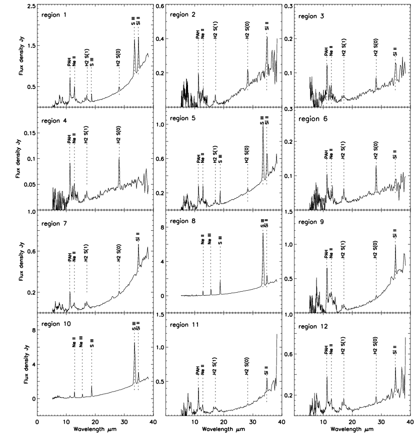
The data reduction pipeline at the Spitzer Science Center was used to reduce and process the raw data products. The details of data reduction method, background subtraction, bad pixel masking and spectral extraction can be found in Kemper et al. (2010). Using the IDL package CUBISM (Smith et al., 2007) the individual spectral orders were combined into spectral cubes and custom software (Sandstrom et al., 2009) was used to merge those spectral cubes. The individual extracted single order spectra (6 for IRS) were merged into a single spectrum using a combination of the overlap regions. The overlap regions in wavelength were used to adjust the flux levels of the spectral orders, except in cases where the S/N of the spectra did not allow for an accurate measurement of the offset in the overlap regions. The background subtraction was made using the dedicated observations of the off-LMC background region. As can be seen in Fig. 1, the area of overlap between SL and LL slits covers a region of 11 arcmin2. The orientation of SL and LL slit apertures is marked on MCELS H image in Fig. 1. The merged spectra were spatially integrated over a circle of radius 30 arcsec within the overlapping area of 11 arcmin2. The overall level of the IRS spectrum in SL and LL was scaled to the photometric fluxes obtained from IRAC 8.0 and MIPS 24, respectively. The photometry was extracted from the latest set of full SAGE-LMC mosaics using the same apertures as were used for the spectroscopy (subtracting the off-LMC background region where appropriate). In general, the MIPS 24 was used to set the overall level of the merged IRS spectrum, supplemented with the IRAC 8.0 data point when it did not impose too strong an offset between the SL and LL orders. A S/N of 10 was achieved for the integrated spectra of each region. The integrated spectra of all twelve regions are shown in Fig. 2.
To study the associated dust properties of these regions, we supplement the analysis with the SAGE-LMC and the Herschel Inventory of The Agents of Galaxy Evolution (HERITAGE) photometric data (Meixner et al., 2013). For the HERITAGE project, the LMC has been surveyed using the Photodetector Array Camera and Spectrometer (PACS; 100 and 160) and the Spectral and Photometric Imaging Receiver (SPIRE; 250, 350, and 500). The details of the observations, data reduction and data processing can be found in Meixner et al. (2010). To extract fluxes we carried out aperture photometry using the aperture photometry tool (APT) and compared the results with the APER routine in IDL. The APT tool performs photometry by summing all pixels within a circular or elliptical aperture. We used a circular aperture of radius 30 arcsec for all twelve sample regions. A background flux of the same aperture size was determined from an off-LMC region, since we want to avoid any contamination of the emission to the background noise. The error on the flux densities comes from source aperture measurements which include background noise obtained by standard deviation of pixels within the sky aperture, and flux calibration errors. To determine the overall uncertainty on the flux density, we quadratically added the flux extraction error and flux calibration errors which are 5 per cent for MIPS, 15 per cent for PACS and 7 per cent for SPIRE data (Meixner et al., 2013).


3 Spectral features
The integrated spectra were decomposed using IDL package PAHFIT (Smith et al., 2007) which can be used to simultaneously fit the PAH features, dust continuum, molecular lines, and fine structure lines. The default PAHFIT package returns only the formal statistical uncertainties for fitted parameters using the given flux uncertainties obtained from the IRS pipeline. We applied a random perturbation method to the existing PAHFIT package to treat better uncertainties for line strengths. We randomly perturbed the flux at each wavelength in a spectrum for a user-specified number of times (100) taking a Gaussian distribution for given standard deviation (). Here, is taken as quadratic sum of flux uncertainties obtained from IRS pipeline and standard deviation () to the continuum. is determined by fitting a polynomial to a user specified region of continuum where no lines are present. We finally applied PAHFIT to each of these perturbed spectra to obtain the distribution of best-fit parameters.
The low-resolution IRS spectra allow us to detect the rotational transition lines of H2, the aromatic band features due to PAH and the fine structure lines of [Ne ii] (12.8), [S iii] (18.7, 33.4) and [Si ii] (34.9). Ten out of the twelve regions showed strong H2 S(0) (=0-0, J=2-0, 28.2) and S(1) (=0-0, J=3-1, 17.0) lines. These lines are detected with a 5 amplitude sensitivity. At shorter wavelengths (5-13) the upper level transitions S(2), S(3), S(4), S(5), S(6) and S(7) (S(2): =0-0, J=4-2, 12.2, S(3): =0-0, J=5-3, 9.6, S(4): =0-0, J=6-4, 8.0, S(5): =0-0, J=7-5, 6.9, S(6): =0-0, J=8-6, 6.1, S(7): =0-0, J=9-7, 5.5) are highly contaminated by aromatic band features of PAHs at 6.2, 7.7, 8.6, 11.3 and 12.6. Fig. 3, 4 and 5 show the best line fits for all detected H2 lines. In regions 3 and 4 the S(2) transition and in region 7 the S(3) transition are strong enough to measure the equivalent widths. These lines are detected with a line strengths of 3. These line fits are also shown in Fig. 3. A 2 upper limit to the integrated intensity was estimated for all remaining non-detected H2 lines. To determine the upper limit intensity, we first subtracted the fit to all PAH features and dust continuum from the observed spectrum. Then we calculated, the root mean square of the residual spectrum at the line within a wavelength range FWHMλ, and the integrated intensity (Ingalls et al., 2011). The measured line intensities of detected H2 lines and upper limits of non-detections are given in Table 2.
The integrated IRS spectra of regions 1, 5, 8 and 10 show strong ionic lines due to [S iii] 18.7, and 33.4, whereas these lines are not detectable in the remaining eight regions. The [Ne iii] 15.1 line is detected in regions 8 and 10 while there is no detection of H2 rotational transitions in these regions. These strong ionic lines indicate the presence of associated H ii regions, hence we examined the environments of those regions using the H map obtained from MCELS which has an angular resolution 3 arcsec. Region 1 is located at the inner edge of northern lobe of H ii region N 148 C in the supergiant shell LMC 3 (Book, Chu & Gruendl, 2008) which is at the northwest of 30 Doradus. Region 5 is located at the northern edge of H ii region N 75 and region 8 is inside N 51 (Bica et al., 1999). Region 10 is located inside the southernmost lobe of H ii region N 55 in the supergiant shell LMC 4 (Dopita, Mathewson & Ford, 1985; Book, Chu & Gruendl, 2008) which is at the northern edge of the LMC. All remaining eight regions appear to be isolated ISM regions in the H image, where [Ne iii] and [S iii] lines are not detected, while the [Si ii] 34.2 and [Ne ii] 12.8 are detected in all the 12 regions.
Our analysis of the regions using H2 rotational lines, H i, H, and CO data will allow us to find out whether these are either molecular or atomic dominated regions or ionized regions. A detailed analysis of spatial distribution of ionic and molecular species of some of these regions along with PDR analysis will be presented in a future paper. In this paper we focus on the properties of H2 emissions detected toward ten regions (Regions 1–7, 9, 11 and 12) discussed above. We have not included regions 8 and 10 in rest of our analysis. In sections 6 and 7 we will also discuss the molecular, atomic and ionized gas contents and physical parameters of dust in these regions. We discuss the analysis of these regions with notations as numbers shown in Fig. 2 and Table 1.

4 H2 column density and excitation temperature
The excitation diagram of H2 rotational emission can be used to derive the level populations and thus excitation temperature of warm molecular hydrogen gas. Using the measured line intensities of each transition we derived the H2 column densities from the following formula:
| (1) |
where are the Einstein coefficients. We assume that the lines are optically thin, the radiation is isotropic and rotational levels of H2 are thermalized. Under these assumptions the level population follow the Boltzmann distribution law at a given temperature and the total H2 column densities can be determined in the Local Thermodynamic Equilibrium (LTE) condition using the formula:
| (2) |
where is the partition function (Herbst et al., 1996).
This function defines a straight line in the excitation diagram with a slope , ie. the upper level column densities normalized with the statistical weight in logarithmic scale as a function of the upper level energy (Goldsmith & Langer, 1999). The statistical weight is , with spin number for even j and for odd j (Rosenthal, Bertoldi & Drapatz, 2000; Roussel et al., 2007). In the LTE condition with gas temperature greater than 300 K, an equilibrium ortho-to-para ratio of 3 is usually assumed. However, for our analysis we adopt an ortho-to-para ratio of 1.7 which is appropriate for gas temperature less than 200 K (Sternberg & Neufeld, 1999). Subsequently, the total column density and temperature are determined by fitting single- or two-temperature models to the excitation diagram. In a two-temperature fit, the first component is used to constrain the column density and temperaure of warm gas and the second component is for hotter gas.
Since we only have two line detections (S(0) and S(1)) for regions 1, 2, 5, 6, 9, 11, 12, and three (S(0), S(1), S(2) or S(3)) for regions 3, 4 and 7 we apply a single-temperature fit to the observed column densities (which is normalized to statistical weight , ) of H2 S(0) and S(1) transitions to constrain the total column density and temperature. We performed a least-square fit to determine the parameters, excitation temperature (from a single-temperature fit) and excited H2 total column density ). The single-temperature fits are shown in solid black lines in the excitation diagrams, Fig. 6, and the derived parameters and ) are given in Table 4. The excitation temperatures () from the single-temperature fits range from . This temperature range corresponds to the ortho-to-para ratio in the range (Fig. 1 in Sternberg & Neufeld 1999), which is consistent with our initial assumption of 1.7.
In reality the ISM is made of gas with a distribution of temperatures. It is very clear from the excitation diagram plot for regions 3, 4 and 7 in Fig. 6 that a single component fit does not pass through the S(2) or S(3) points. This indicates that in general a multiple-temperature fit is needed for characterizing the excitation diagrams. It should also be noted that introducing a second temperature in the fit may lower the excitation temprature of cooler component relative to the single-temperature fit. Since the determination of the total column density is very sensitive to the excitation temperature, we might underestimate the total column density in a single-temperature fit. In order to check these discrepancies we performed a two-temperature model fit to regions 3, 4 and 7. Although we have a measurement of third transition for these three regions, in order to approximate a two-temperature fit we need measurements for at least four transitions. Nevertheless, using these three detections and upper limit measurements for higher transitions we constrained the hot gas column densities and temperature by fitting a two-temperature model for these three regions. The two-temperature model fits in regions 3, 4 and 7 give the temperature for hot gas as 750, 1100 and 630 K respectively. These fits are shown as dotted black lines in the excitation diagrams of regions 3, 4 and 7 in Fig. 6 and the derived parameters two,1 (low temperature component from two-temperature fit), two,2 (high temperature component from two-temperature fit), are shown in Table 4. Note that the excitation temperature two,1 derived from two-component fit is slightly lowered compared with single-temperature fit. As we have not detected any S(2) or S(3) lines for regions 1, 2, 5, 6, 9, 11 and 12, and the two-temperature fit through upper limit measurements only helps us to constrain an upperlimit excitation temperature of a possible warmer component we use the column densities, ), determined from single-temperature fit to estimate gas masses. Moreover, the second component contributes a negligible fraction to the total column density. The derived masses are given in Table. 4. Note that we may underestimate the mass if a second components is required, because inclusion of second component can increase the final column densities. In order to estimate this discrepancy, we compared the masses derived from single-temperature and two-temperature fits for regions 3, 4 and 7. The two-temperature fit increases the mass by a factor of 25 per cent compared to the single-temperature fit.
5 Comparison of warm H2 with PAH and IR emission

In order to quantify the importance of warm H2 gas and thereby to constrain possible excitation mechanism, we compare the power emitted in H2 with the dust emission traced in the form of PAH (traced by IRAC 8.0 band emission), 24 and total infrared (TIR) surface brightness. The TIR surface brightness is determined by combining the IRAC 8.0, MIPS 24, 70 and 160 flux densities using equation11 1 TIR (22) in Draine & Li (2007). Perhaps, the scattered light from stellar emission could make a significant contribution to the 8.0 fluxes. According to J. Seok (private communication), the contribution of scattered starlight in the 8.0 band in the H ii region of the LMC is 10 per cent. Hence, we assume that the contribution of starlight to the 8.0 band emission is less than 10 per cent for our sample regions.
In Fig. 7 we examine the relation between power emitted in the sum of H2 S(0) and S(1) lines with the power emitted at IRAC 8.0 band, which traces the PAH 7.9 emission in the ISM. For comparison we show the SINGS galaxy samples (Roussel et al., 2007) and Galactic translucent clouds (Ingalls et al., 2011) along with our ten LMC regions. The ratio of the H2 S(0) and S(1) lines to the 7.9 PAH emission shows very little deviation for all ten LMC regions, and agrees well with the SINGS normal galaxy samples. In Fig. 7 a we demonstrate that the relation between H2 and PAH emission can be fitted with the function log log with a correlation coefficient of R0.96, following the strong correlation between H2 and PAH emission in SINGS normal galaxies earlier reported by Roussel et al. (2007). In Fig. 7 the LMC samples are located along with the dwarf galaxies and these line-up with the star-forming galaxies. If both H2 and PAHs are excited in PDRs, such a tight correlation between H2 and PAH emission is expected (Rigopoulou et al., 2002). In PDRs, the PAHs are significant contributors to the photo-electric heating and H2 emission is expected at the edge of the PDR. In the classic PDR of the Orion Bar, it has been found that the H2 emission is spatially adjacent to the PAH emission (Tielens et al., 1993). In our observations, we do not resolve the PDR layers; however, we expect the H2 and PAH emission to be correlated if the H2 emission arises from a PDR. It should also be noted here that, PDRs can be formed in any neutral medium illuminated by FUV radiation where the radiation field is low, compared to the intense radiation in star-forming regions. In such regions, this kind of tight correlation between H2 and PAH emission is expected, even though the radiation field intensity is much lower (Roussel et al., 2007).
Ingalls et al. (2011) have found excess H2 emission compared to PAHs in Galactic translucent clouds. They conclude that H2 emission is dominated by mechanical heating even in non-active galaxies. This kind of excess H2 emission has also been reported in various other objects, such as active galactic nuclei and ultraluminous infrared galaxies (Ogle et al., 2010; Higdon et al., 2006). They argue that an additional excitation mechanism, possibly shock or gas heating by X-ray, might be responsible for the excess emission of H2. Such a heating mechanism can produce a relatively larger enhancement of the warm H2 compared to the UV excitation in PDRs. In contrast, we argue that H2 in the observed ISM of the LMC is dominated by FUV photo-processes.

In Fig. 8 b we plot the ratio of power emitted in the sum of S(0) and S(1) lines to TIR power. Roussel et al. (2007) reported that the H2/TIR ratio is remarkably constant for their sample of normal galaxies, and also in good agreement with the prediction from PDR models by Kaufman, Wolfire & Hollenbach (2006). Again, the LMC regions are shown along with the SINGS dwarf galaxies and star-forming galaxies for comparison. As in Fig. 7, the LMC sources have a similar trend as the SINGS galaxies, but larger scatter. The ratio of H2/TIR power ranges over 0.0001 to 0.001. It is noted that the LMC points are offset towards higher H2/TIR ratios relative to the dwarf galaxies, whereas they are consistent with the H2/PAH ratios (Fig. 7). In Fig. 8 a we show that the relation between H2 and TIR can be fitted to a funtion log log with a correlation coefficient 0.92. In PDRs, the FUV radiation from young stars heats the dust grains and give rise to infrared continuum radiation or mid-infrared cooling lines such as H2 rotational or fine structure lines; hence we expect a strong tendency to increase in H2 emission with increase in total infrared flux. The ratio of fine structure line [O i] flux to TIR flux, [O i]/TIR, has been used as a diagnostic for the photo-electric heating efficiency in a variety of environments of the LMC and SMC by van Loon et al. (2010a); van Loon et al. (2010b).
In order to investigate the relation of H2 emission with the 24 continuum emission, we plot the power ratio H2/24 as a function of 24 power in Fig. 9 a. In star-forming galaxies, the H2 luminosity correlates with the 24 emission that traces the amount of star formation (Roussel et al., 2007). The H2/24 ratio decreases with increase in 24 emission, with a large scatter, in Fig. 9 a. Note that here we compare the H2 and 24 emission of ten different regions of the LMC with those in SINGS galaxies. This anti-correlation may indicate that globally, the 24 emission traces a significantly different, mostly uncorrelated medium from the warm H2 gas, in contrast to the PAH 7.9 emission (see Fig. 7). In order to better understand this relation, in Fig. 9 b we plot the power ratio 7.9/24 as a function of 24 power. This plot clearly shows an anti-correlation dependency of PAH emission with 24 emission. This trend could be due to the increased starlight intensities in regions where the 24 emission is higher (Draine & Li, 2007), or even combined with the preferential destruction of small PAHs in these regions (Draine & Li, 2001). If the starlight intensity is sufficiently high, the dust (i.e., nano dust) which emits at 24 is no longer in the regime of single-photon heating. Therefore increases with , while the 7.9 emitter (PAHs) is still in the regime of single-photon heating. Hence does not vary with (see Fig. 13 b of Draine & Li 2007), and intends to decrease with and . Furthermore, we cannot rule out the possibility that the 7.9 emitter may be partly destroyed at higher , which would also lead to a decrease of power ratio 7.9/24 with 24 power. If PAHs are partly destroyed one would expect a decreased photo-electric heating of H2 and thus a decrease of power ratio H2/24 with 24 power and .

6 Warm H2, cold H2, H i and H: phases of the ISM
We can compare the amount of gas contained in the warm component with the major phases of hydrogen: cold molecular H2, atomic H i, and ionized H+. The cold H2 gas mass is derived using CO (J=1-0) line observations (Wong et al., 2011) obtained with the Magellanic Mopra Assessment (MAGMA) and the NANTEN surveys (Fukui et al., 2008). As part of MAGMA project the LMC has been surveyed in CO (J=1-0) line with the 22 m Mopra telescope of the Australian Telescope National Facility (Wong et al., 2011). This observation achieved a 45 arcsec angular resolution with a sensitivity nearly 0.4. At this angular resolution, the Mopra CO intensity map is sufficient for our analysis. However, the MAGMA survey does not cover the whole LMC, as it was a targeted follow-up survey of the LMC regions where significant CO emission is detected in the previous NANTEN CO(J=1-0) survey with angular resolution 2.6 arcmin. Hence, we have to use the NANTEN CO intensities for at least five regions where no MAGMA observations exist. The CO integrated intensities were extracted over a 30 arcsec radius aperture size. These integrated intensities () were then converted to H2 (cold) column densities assuming the Galactic CO-to-H2 conversion factor of 210 (Bolatto, Wolfire & Leroy, 2013).
The atomic gas is traced by line emission observations by the Australia Telescope Compact Array (ATCA) and Parkes single dish telescope spanning 11.1 12.4 deg2 on the sky at a spatial resolution 1 arcmin (Kim et al., 2003). The construction of a H i intensity map from the H i data cube and further conversion to column density is discussed by Bernard et al. (2008). We integrated the H i column densities within an aperture radius 30 arcsec. The derived H i column densities and masses are given in Table 5.
The ionized gas is traced by the H emission observed in the Southern H-Alpha Sky Survey Atlas (SHASSA; Gaustad et al. (2001)) carried out at the Cerro Tololo Inter-American Observatory in Chile. The angular resolution of that image is 0.8 arcmin with a sensitivity level of 2 Rayleighs, where 1 Rayleigh = for Te= (Dickinson, Davies & Davis, 2003), corresponding to erg s-1cm-2 sr-1. In order to determine the H+ column density, we first calculated the electron density using the formula EM=L (Dickinson, Davies & Davis, 2003), where EM is the emission measure and L is the path length in parsec. We assume here the width of emission feature is the same as the emitting path length along the line of sight. Consequently, the H+ column density is calculated from the H intensity and electron density of each region using equation22 2 (3) (6) reported by Bernard et al. (2008).
Our main purpose here is to estimate what fraction of warm H2 takes up the total gas, compared to the other phases of the ISM represented by cold H2, H i and H+. Mass fractions in atomic, ionic, warm H2 and cold H2 form are given in Table 5 and a histogram is shown in Fig. 10. The warm H2 mass fraction varies slightly from region to region with a significant contribution per cent to the total gas mass. The histogram in Fig. 10 compares the fraction of H i, warm H2 and cold H2 in ten regions where H2 excitation is detected. Region 5 shows the largest amount of warm H2, 17 per cent of the total gas mass (see Table 5), with atomic gas and cold H2 masses at nearly 31 per cent and 50 per cent respectively. Warm H2 is per cent of the total gas mass in regions 1, 2, 7, 9 and 12. The H2 traced by NANTEN CO is very negligible and the atomic gas is per cent of the total gas (see Table 5) in regions 7, 9, 11 and 12. In particular, regions 1, 2, 7, 9, 11 and 12 are diffuse atomic, where H i is the dominant ISM component, while regions 3, 4, 5 and 6 are molecular dominated. The amount of warm H2 is equally important in both atomic and molecular dominated regions. In most regions only two lines are detected, hence the mass of warm H2 could be underestimated. In fact, a large uncertainty is expected in the determination of cold H2 mass from CO. The first dominant uncertainty comes from matching the size of the region over which the IRS spectrum was integrated with two different beam sizes for CO observations obtained from Mopra and NANTEN telescopes. Since, the CO luminosity for regions 2, 9, 11 and 12 were extracted from NANTEN CO map with angular resolution 2.6 arcmin, we expect a large uncertainty in the cold H2 mass for those regions. Another source of uncertainty comes from the CO-to-H2 conversion factor for which we used a Galactic value of 210 according to Bolatto, Wolfire & Leroy (2013). Note that the CO-to-H2 conversion factor strongly depends on metallicity which we assumed uniform over the regions and the applicability of the Galactic value is debated.


7 Comparison of warm H2 with dust
An important ISM component that is closely linked to the formation of H2 is dust. Hence, for a first approximation here we try to determine the physical parameters of dust by fitting modified blackbody curves to the far-infrared spectral energy distributions (SEDs). We determine the temperature and mass of the dust by fitting a single-temperature modified blackbody curve to the far-infrared SED obtained from Herschel photometric observations. PACS (100 and 160 ) and SPIRE (250, 350 and 500 ) fluxes are fitted with the modified blackbody curve, following the method outlined in Gordon et al. (2010). We restrict our SED fitting above 70 as we assume the dust grains are in thermal equilibrium with the radiation field. In our fitting method, the emissivity is allowed to vary between 1 2.5 (Gordon et al., 2014). The uncertainties in mass and temperature come from SED fitting, where quadratic sum of uncertainties in flux extraction from photometric images and absolute error in flux calibration are adopted (Meixner et al., 2013). The fluxes are randomly perturbed within a Gaussian distribution of uncertainties and chi-square fits are used to determine dust mass and temperature. The measurements are given in Table. 5. The dust shows a range in mass 15M90 M⊙ within the 1 arcmin integrated region and in temperature 1528.
In the far-infrared domain, the emission is dominated by cold large grains which are in thermal equilibrium with the radiation field. Therefore the spectrum can be approximated with a modified blackbody curve. This is not well constrained for mid-infrared continuum, where the emission is dominated by small grains and PAHs. Moreover, the modified blackbody fits are known to underestimate the dust by a factor of nearly 0.7 in most regions of the LMC (Galliano et al., 2011). Hence, in order to constrain the total dust mass with better uncertainties, we fitted the SEDs in the wavelength range from 8.0 to 500 (combining the IRAC, MIPS and Herschel SPIRE bands) with the Galliano et al. (2011) model using a least-square approach and Monte-carlo error propagation. More details of fitting and dust parameter determination can be found in Galliano et al. (2011). The derived total dust masses M are given in Table 5 for comparison with the dust mass derived from single-temperature blackbody fits. It should be noted that, error bars on dust mass derived from this method are highly asymmetric (Table 5). In addition, we derive the average starlight intensity using equation (9) of Galliano et al. (2011): this parameter is on first approximation related to the grain equilibrium temperature by .
In Fig. 11 we examine the relation of warm H2 with the dust parameters derived by different methods explained above. No clear relation is noticed for the warm H2 mass with dust mass derived by fitting a blackbody curve to far-infrared SED (Fig. 11 a). The warm H2 mass fraction (in terms of the total H2 mass) is found to be positively correlated (R0.76) with the dust equilibrium temperature (Fig. 11 b). Fig. 11 c and d show that the H2 mass fraction and excitation temperature are positively correlated (R0.80) with the average starlight intensity , which is a measure of dominant input energy for dust heating in the medium. These correlation tests confirm that photo-electric heating in the PDR is efficient to excite H2 in both atomic and molecular dominated diffuse regions. In Fig. 11 e, the warm H2 mass shows a moderate positive correlation (R0.70) with the total dust mass, derived by fitting infrared SED with the Galliano et al. (2011) model. Since we compare dust mass with the H2 mass, we attempt to remove the dust associated with H i from the total dust mass. Hence, we subtract a factor ZdM(H i) from dust mass where Zd is dust-to-gas ratio and M(H i) is total H i gas mass.
| Region | S (0) | S(1) | S(2) | S(3) | S(4) | S(5) | S(6) | S(7) | 7.9 | 24 | TIR |
|---|---|---|---|---|---|---|---|---|---|---|---|
| 10-09 | 10-09 | 10-09 | 10-09 | 10-09 | 10-09 | 10-09 | 10-09 | 10-07 | 10-08 | 10-06 | |
| 1 | 2.2(0.3) | 2.5(0.3) | 7.54(2.5) | 13.6(0.01) | 9.92(0.2) | ||||||
| 2 | 1.9(0.8) | 1.3(0.7) | 4.01(0.2) | 3.43(0.01) | 3.02(0.06) | ||||||
| 3 | 0.62(0.2) | 0.18(0.1) | 0.15(0.03) | 2.32(0.4) | 2.70(0.005) | 2.33(0.3) | |||||
| 4 | 0.80(0.4) | 0.30(0.03) | 0.60(0.5) | 1.78(0.8) | 1.60(0.005) | 1.60(0.3) | |||||
| 5 | 1.3(0.7) | 1.3(0.5) | 3.98(0.6) | 6.25(0.002) | 4.63(0.6) | ||||||
| 6 | 1.2(0.2) | 0.72(0.2) | 2.69(0.7) | 1.90(0.006) | 2.43(0.03) | ||||||
| 7 | 0.62(0.1) | 0.9(0.3) | 1.4(0.08) | 4.16(0.5) | 5.11(0.01) | 5.29(0.06) | |||||
| 9 | 0.73(0.3) | 1.5(0.3) | 5.48(2.5) | 5.64((0.007) | 8.01(0.08) | ||||||
| 11 | 0.51(0.2) | 0.58(0.3) | 4.12(1.5) | 5.92(0.01) | 5.03(0.06) | ||||||
| 12 | 1.2(0.3) | 1.3(0.4) | 3.16(0.5) | 3.86(0.006) | 3.70(0.1) |
| Region | S (0) | S(1) | S(2) | S(3) | S(4) | S(5) | S(6) | S(7) |
| 1019 | 1017 | 1016 | 1016 | 1015 | 1015 | 1015 | 1015 | |
| 1 | 1.4(0.15) | 6.7(0.5) | ||||||
| 2 | 1.2(0.5) | 3.1(1.7) | ||||||
| 3 | 0.38(0.09) | 0.42(0.3) | 0.42(0.07) | |||||
| 4 | 0.47(0.22) | 0.67(0.06) | 1.6(1.4) | |||||
| 5 | 0.80(0.4) | 3.0(1.1) | ||||||
| 6 | 0.96(0.13) | 0.92(0.2) | ||||||
| 7 | 0.38(0.08) | 2.2(0.6) | 0.87(0.05) | |||||
| 9 | 0.45(0.2) | 3.5(0.7) | ||||||
| 11 | 0.31(0.13) | 1.3(0.6) | ||||||
| 12 | 0.78(0.19) | 2.9(0.98) |
| Reg | M(H | ||||
|---|---|---|---|---|---|
| M⊙ | |||||
| K | K | K | 1020 | 103 | |
| 1 | |||||
| 2 | |||||
| 3 | |||||
| 4 | |||||
| 5 | |||||
| 6 | |||||
| 7 | |||||
| 9 | |||||
| 11 | |||||
| 12 | |||||
| Reg | 1M | 2M | (H i) | M(H i) | 3 | M(H | 4Mtot | f(H i) | f(H+) | f(H | f(H) | |
|---|---|---|---|---|---|---|---|---|---|---|---|---|
| 1021 | 103 | 1021 | 103 | 103 | ||||||||
| K | M⊙ | M⊙ | M⊙ | M⊙ | M⊙ | |||||||
| 1 | 148 | 4.8 | 6.4 | 1.6 | 12.0 | 0.53 | 0.004 | 0.11 | 0.36 | |||
| 2 | 40 | 3.7 | 5.0 | 8.7 | 0.57 | 0.002 | 0.14 | 0.29 | ||||
| 3 | 40 | 2.1 | 2.8 | 2.3 | 9.7 | 0.30 | 0.08 | 0.63 | ||||
| 4 | 99 | 2.1 | 2.8 | 2.6 | 10.5 | 0.27 | 0.08 | 0.65 | ||||
| 5 | 66 | 1.5 | 2.0 | 1.2 | 6.5 | 0.31 | 0.01 | 0.17 | 0.50 | |||
| 6 | 44 | 3.2 | 4.3 | 1.9 | 10.3 | 0.41 | 0.09 | 0.50 | ||||
| 7 | 22 | 4.1 | 5.5 | 6.0 | 0.92 | 0.002 | 0.08 | |||||
| 9 | 54 | 4.6 | 6.2 | 6.8 | 0.90 | 0.004 | 0.08 | 0.02 | ||||
| 11 | 66 | 6.4 | 8.6 | 9.2 | 0.93 | 0.002 | 0.05 | 0.02 | ||||
| 12 | 49 | 2.9 | 4.0 | 4.8 | 0.81 | 0.005 | 0.15 | 0.03 |
1: Dust mass determined by fitting single-temperature modified blackbody curve. 2: Dust mass determined by fitting the infrared SEDs with Galliano et al. (2011) model. 3: Cold molecular hydrogen column density calculated for Galactic X factor, Xco,20 = . 4: Total gas mass which is the sum of H i, H+, warm H2 and cold H2 gas masses. 5: From NANTEN CO observations.
8 Summary
We report molecular hydrogen emission toward ten ISM regions in the LMC, observed with the Spitzer IRS as part of the SAGE-spec project. For our analysis, the low-resolution infrared spectra of 12 regions were extracted from IRS spectral cubes and integrated over a circular region with radius 30 arcsec. All these twelve regions are either isolated diffuse regions or associated with H ii regions in the LMC (see Fig. 1). The pure rotational 0–0 transitions of H2 were detected in the spectra toward ten regions. The excitation diagram analysis of the detected H2 transitions gives constraints on the warm H2 gas mass and temperature. We have only two line detections for most of the regions, hence we performed single-temperature fit to the excitation diagram. For three regions a third H2 line is detected, allowing for a two-temperature fit. In addition to mass and excitation temperature of the warm H2, we derived mass (within the 30 arcsec circular region) of H+ from H emission; and mass of H i and cold H2 from ancillary H i and CO data respectively. These measurements allow us to distinguish the regions which are diffuse atomic and molecular. We have also determined the dust temperature and mass from infrared SED fitting, in order to compare with the warm H2 gas parameters.
- •
Our analysis shows that six regions (regions 1, 2, 7, 9, 11, 12) are diffuse atomic in nature where H i is the dominant ISM component 50 per cent while four other regions (regions 3, 4, 5 and 6) are diffuse molecular, where H2 is dominant (50 per cent; see Fig. 10). In both cases, warm H2 contributes a significant fraction to the total ISM gas, with a mass of per cent of the total gas mass and excitation temperature . Interestingly, the amount of warm H2 is found to be equally significant in both atomic and molecular dominated environments, regardless of the nature of the region.
- •
For all ten LMC regions where clear H2 excitation is detected, a tight correlation between the H2 and 7.9 PAH emission is found (R0.96). This indicates a PDR excitation, caused by photo-electrons ejected from PAHs by UV radiation. The surface brightness ratio H2/PAH shows very little deviation () which agrees with the SINGS normal galaxy samples (Roussel et al., 2007).
- •
The surface brightness ratio H2/TIR shows relatively larger scatter compared with the SINGS galaxy samples, but a strong correlation is observed between H2 and TIR power with a correlation coefficient of 0.92. Since the TIR flux is an approximate measure of the input energy into the medium, this relation may represent more efficient photo-electric heating in the environment where H2 is excited.
- •
The ratio H2/24 is found to decrease with an increase in 24 power. A similar anti-correlation is also found for PAH emission. The ratio 7.9/24 decreases with the 24 power. This could be due to the increased starlight intensity or to the preferential destruction of PAHs at higher 24 emission. On the other hand, it may also be possible that the 24 and H2 emission arise from physically unrelated regions.
- •
We examined various tests for correlation of warm H2 mass and excitation temperature with the ISM dust parameters (see Fig. 11). There is a moderate positive correlation for the H2 mass with the cold dust mass. The warm H2 mass fraction tends to positively correlate with the cold dust equilibrium temperature or average starlight intensity .
9 Acknowledgement
F.K acknowledges funding from Taiwan’s Ministry of Science and Technology (MoST) under grants NSC100-2112-M-001-023-MY3 and MOST ISO-2112-M-001-033. We thank the referee for fruitful comments.
References
- Beirão et al. (2009) Beirão P., Appleton P. N., Brandl B. R., Seibert M., Jarrett T., Houck J. R., 2009, ApJ, 693, 1650
- Beirão et al. (2012) Beirão P. et al., 2012, ApJ, 751, 144
- Bernard et al. (2008) Bernard J.-P., Reach W. T., Paradis D., Meixner M., Paladini R. e. a., 2008, AJ, 136, 919
- Bica et al. (1999) Bica E. L. D., Schmitt H. R., Dutra C. M., Oliveira H. L., 1999, AJ, 117, 238
- Bolatto, Wolfire & Leroy (2013) Bolatto A. D., Wolfire M., Leroy A. K., 2013, ARAA, 51, 207
- Book, Chu & Gruendl (2008) Book L. G., Chu Y.-H., Gruendl R. A., 2008, ApJS, 175, 165
- Dickinson, Davies & Davis (2003) Dickinson C., Davies R. D., Davis R. J., 2003, MNRAS, 341, 369
- Dopita, Mathewson & Ford (1985) Dopita M. A., Mathewson D. S., Ford V. L., 1985, ApJ, 297, 599
- Draine & Li (2001) Draine B. T., Li A., 2001, ApJ, 551, 807
- Draine & Li (2007) Draine B. T., Li A., 2007, ApJ, 657, 810
- Draine, Roberge & Dalgarno (1983) Draine B. T., Roberge W. G., Dalgarno A., 1983, ApJ, 264, 485
- Fukui et al. (2008) Fukui Y. et al., 2008, ApJS, 178, 56
- Galliano et al. (2011) Galliano F. et al., 2011, A&A, 536, A88
- Gaustad et al. (2001) Gaustad J. E., McCullough P. R., Rosing W., Van Buren D., 2001, PASP, 113, 1326
- Goldsmith & Langer (1999) Goldsmith P. F., Langer W. D., 1999, ApJ, 517, 209
- Gordon et al. (2010) Gordon K. D. et al., 2010, A&A, 518, L89
- Gordon et al. (2014) Gordon K. D. et al., 2014, ArXiv e-prints
- Habart et al. (2005) Habart E., Walmsley M., Verstraete L., Cazaux S., Maiolino R., Cox P., Boulanger F., Pineau des Forêts G., 2005, SSR, 119, 71
- Herbst et al. (1996) Herbst T. M., Beckwith S. V. W., Glindemann A., Tacconi-Garman L. E., Kroker H., Krabbe A., 1996, AJ, 111, 2403
- Higdon et al. (2006) Higdon S. J. U., Armus L., Higdon J. L., Soifer B. T., Spoon H. W. W., 2006, ApJ, 648, 323
- Hollenbach & Tielens (1997) Hollenbach D. J., Tielens A. G. G. M., 1997, ARAA, 35, 179
- Hunt et al. (2010) Hunt L. K., Thuan T. X., Izotov Y. I., Sauvage M., 2010, ApJ, 712, 164
- Ingalls et al. (2011) Ingalls J. G., Bania T. M., Boulanger F., Draine B. T., Falgarone E., Hily-Blant P., 2011, ApJ, 743, 174
- Kaufman, Wolfire & Hollenbach (2006) Kaufman M. J., Wolfire M. G., Hollenbach D. J., 2006, ApJ, 644, 283
- Kemper et al. (2010) Kemper F. et al., 2010, PASP, 122, 683
- Kennicutt et al. (2003) Kennicutt, Jr. R. C. et al., 2003, PASP, 115, 928
- Kim et al. (2003) Kim S., Staveley-Smith L., Dopita M. A., Sault R. J., Freeman K. C., Lee Y., Chu Y.-H., 2003, ApJS, 148, 473
- Madden et al. (1997) Madden S. C., Poglitsch A., Geis N., Stacey G. J., Townes C. H., 1997, ApJ, 483, 200
- Meixner et al. (2010) Meixner M. et al., 2010, A&A, 518, L71
- Meixner et al. (2013) Meixner M. et al., 2013, AJ, 146, 62
- Ogle et al. (2010) Ogle P., Boulanger F., Guillard P., Evans D. A., Antonucci R., Appleton P. N., Nesvadba N., Leipski C., 2010, ApJ, 724, 1193
- Pietrzyński et al. (2013) Pietrzyński G., Graczyk D., Gieren W., Thompson I. B., Pilecki B., Udalski A., Soszyński I., 2013, Nature, 495, 76
- Rigopoulou et al. (2002) Rigopoulou D., Kunze D., Lutz D., Genzel R., Moorwood A. F. M., 2002, A&A, 389, 374
- Rosenthal, Bertoldi & Drapatz (2000) Rosenthal D., Bertoldi F., Drapatz S., 2000, A&A, 356, 705
- Roussel et al. (2007) Roussel H. et al., 2007, ApJ, 669, 959
- Sandstrom et al. (2009) Sandstrom K. M., Bolatto A. D., Stanimirović S., Smith J. D. T., van Loon J. T., Leroy A. K., 2009, in IAU Symposium, Vol. 256, IAU Symposium, Van Loon J. T., Oliveira J. M., eds., pp. 160–165
- Smith et al. (2007) Smith J. D. T., Draine B. T., Dale D. A., Moustakas J., Kennicutt, Jr. R. C., Helou G., Murphy E. J., Walter F., 2007, ApJ, 656, 770
- Smith & MCELS Team (1998) Smith R. C., MCELS Team, 1998, PASA, 15, 163
- Sternberg & Neufeld (1999) Sternberg A., Neufeld D. A., 1999, ApJ, 516, 371
- Tielens et al. (1993) Tielens A. G. G. M., Meixner M. M., van der Werf P. P., Bregman J., Tauber J. A., Stutzki J., Rank D., 1993, Science, 262, 86
- van Loon et al. (2010a) van Loon J. T. et al., 2010a, AJ, 139, 68
- van Loon et al. (2010b) van Loon J. T., Oliveira J. M., Gordon K. D., Sloan G. C., Engelbracht C. W., 2010b, AJ, 139, 1553
- Wolfire, Hollenbach & McKee (2010) Wolfire M. G., Hollenbach D., McKee C. F., 2010, ApJ, 716, 1191
- Wong et al. (2011) Wong T., Hughes A., Ott J., Muller E., Pineda J. L., Bernard J.-P. e. a., 2011, ApJS, 197, 16