Estimating the Accuracies of Multiple Classifiers Without Labeled Data
Abstract
In various situations one is given only the predictions of multiple classifiers over a large unlabeled test data. This scenario raises the following questions: Without any labeled data and without any a-priori knowledge about the reliability of these different classifiers, is it possible to consistently and computationally efficiently estimate their accuracies? Furthermore, also in a completely unsupervised manner, can one construct a more accurate unsupervised ensemble classifier? In this paper, focusing on the binary case, we present simple, computationally efficient algorithms to solve these questions. Furthermore, under standard classifier independence assumptions, we prove our methods are consistent and study their asymptotic error. Our approach is spectral, based on the fact that the off-diagonal entries of the classifiers’ covariance matrix and 3-d tensor are rank-one. We illustrate the competitive performance of our algorithms via extensive experiments on both artificial and real datasets.
1 Introduction
Consider a classification problem from an instance space to an output label set . In contrast to the classical supervised setting, in various contemporary applications, one has access only to the predictions of multiple experts or classifiers over a large number of unlabeled instances. Moreover, the reliability of these experts may be unknown, and at test time there is no labeled data to assess it. This occurs for example when due to privacy considerations each classifier is trained with its own possibly proprietary labeled data, unavailable to us. Another scenario is crowdsourcing, where an annotation task over many instances is distributed to many annotators whose reliability is a-priori unknown, see for example Welinder et al. (2010); Whitehill et al. (2009); Sheshadri and Lease (2013). This setup, denoted as unsupervised-supervised learning in Donmaz_2010, appears in several other application domains, including decision science, economics and medicine, see Snow et al. (2008); Raykar et al. (2010); Parisi et al. (2014).
Given only the matrix or a significant part of it, with holding the predictions of the given classifiers over instances, and without any labeled data, two fundamental questions arise: (i) Under the assumption that different classifiers make independent errors, is it possible to consistently estimate the accuracies of the classifiers in a computationally efficient way; and (ii) is it possible to construct, again by some computationally efficient procedure, an unsupervised ensemble learner, more accurate than most if not all of the original classifiers.
The first question is important in cases where obtaining the predictions of these classifiers is by itself an expensive task, and after collecting a certain number of instances and their predictions, we wish to pick only a few of the most accurate ones, see Rokach (2009). The second question, also known as offline consensus, is of utmost importance in improving the quality of automatic decision making systems based on multiple sources of information.
Beyond the simplest approach of majority voting, perhaps the first to define and address these questions were Dawid and Skene (1979). With the increasing popularity of crowdsourcing and large scale expert opinion systems, the last years have seen a surge of interest in these problems, see Sheng et al. (2008); Whitehill et al. (2009), Raykar et al. (2010), Platanios et al. (2014) and references therein. Yet, the most common methods to address questions (i) and (ii) above are based on the expectation maximization (EM) algorithm, already proposed in this context by Dawid and Skene, and whose only guarantee is convergence to a local maxima.
Two recent exceptions, proposing spectral (and thus computationally efficient) methods with strong consistency guarantees are Karger et al. (2011) and Parisi et al. (2014). Karger et al. (2011) assume a spammer-hammer model, where each classifier is either perfectly correct or totally random and develop a spectral method to detect which one is which. Parisi et al. (2014) derive a spectral approach to address questions (i) and (ii) above in the context of binary classification. Their approach, however, has several limitations. First, they do not actually estimate each classifier sensitivity and specificity, but only show how to consistently rank them according to their balanced accuracies. Second, their unsupervised learner assumes that all classifiers have balanced accuracies close to 1/2 (random). Hence, their ensemble learner may be suboptimal, for example, when few classifiers are significantly more accurate than all others.
In this paper we extend and generalize the results of Parisi et al. (2014) in several directions and make the following contributions: In Sec. 3, focusing on the binary case, we present a simple spectral method to estimate the sensitivity and specificity of each classifier, assuming the class imbalance is known. Hence, the problem boils down to estimating a single-scalar – the class imbalance. In Section 4 we present two different methods to do so. First, in Sec. 4.1, we prove that the off-diagonal elements of the covariance matrix and the joint covariance tensor of the set of classifiers are both rank 1. Moreover the covariance matrix and tensor share the same eigenvector but with different eigenvalues, from which the class imbalance can be extracted by a simple least-squares procedure. In Sec. 4.2, we devise a second algorithm to estimate the class imbalance by a restricted likelihood approach. The maxima of this function is attained at the class imbalance, and can thus be found by a one-dimensional scan. Both algorithms are computationally efficient, and under the assumption that classifiers make independent errors, are also proven to be consistent. For the first method, we also prove it is rate optimal with asymptotic error , where is the number of unlabeled samples. Our work thus provides a simple and elegant solution to the long-standing problem originally posed by Dawid and Skene [2], whose previous solutions were mostly based on expectation maximization approaches to the full likelihood function.
In Sec. 5 we consider the multiclass case. Building upon standard reductions from multiclass to binary, we devise a method to estimate the class probabilities and the diagonal entries of the confusion matrices of all classifiers. We also prove that in the multiclass case, using only the first and second moments of these binary reductions, it is in general not possible to estimate all entries of the confusion matrices of all classifiers. This motivates the development of tensor or higher order methods to solve the multi-class case, as for example in Zhang et al. (2014). In Sec. 6 we illustrate our methods on both real and artificial data. The results on real data show that our proposed ensemble learner achieves a competitive performance even in practical scenarios where the assumption of independent classifiers’ errors does not hold precisely.
Related Work
Under the assumption that all classifiers make independent errors, the crowdsourcing problem we address is equivalent to learning a mixture of discrete product distributions. This problem was studied, among others, by Freund and Mansour (1999) for the case of distributions, and by Feldman et al. (2008) for . Important observations regarding the low-rank spectral structure of the second and third moments of such distributions were made by Anandkumar et al. (2012a); Anandkumar et al. (2012b). Building upon these results, recently Jain and Oh (2013) and Zhang et al. (2014), devised computationally efficient algorithms to estimate the parameters of the mixture of product distributions, which are equivalent to the confusion matrices and class probabilities in our problem.
Our first method to estimate the class imbalance in the binary case using the mean-centered 3-d tensor is closely related to these works, with some notable differences. One key difference is that the above works study non-centered tensors of classifiers’ outputs, and hence for a k-class problem, need to resolve the structure of rank-k tensors. In contrast, we work with centered matrices and tensors. In the binary case with we thus obtain a simpler rank-1 tensor, which we do not even need to decompose, but only extract a single scalar from it. A second difference is that the above methods require stronger assumptions on the classifiers. For example, Zhang et al. (2014) divide the classifiers into groups and assume that within each group, on average classifiers are better than random. Due to these differences, our resulting algorithm is significantly simpler.
Our second algorithm for estimating the class imbalance, based on a restricted likelihood approach is totally different from these tensor-based works, as it requires only a spectral decomposition of the classifiers’ covariance matrix, and then optimizes a 1-d function of the full likelihood of the data. On both simulated and real data, this second approach had at least as good as, and in some cases better accuracy compared to the tensor based method. Finally, while we focus on classification, our algorithms may also be of interest to learning a mixture of discrete product distributions.
2 Problem Setup
We consider the following binary classification problem, as also studied in several works (Dawid and Skene (1979); Raykar et al. (2010); Parisi et al. (2014)). Let be an instance space with an output space . A labeled instance is a realization of the random variable which has an unknown probability density and and marginals and respectively. We further denote by the class imbalance of ,
Let be classifiers operating on . In this binary setting, the accuracy of the -th classifier is fully specified by its sensitivity and specificity ,
For future use, we denote by its balanced accuracy,
In this paper we consider the following totally unsupervised scenario. Let be a matrix with entries , where is the label predicted at instance by classifier . In particular, we assume no prior knowledge about the classifiers, so their accuracies (sensitivities and specificities ) are all unknown.
Given only the matrix of binary predictions11 1 For simplicity of exposition, we assume the matrix is fully observed. While beyond the scope of this paper, our proposed methods and theory continue to hold if few entries are missing (at random), such that accurate estimates of various means, covariances and tensors, as detailed in Sections 3-4 are still possible. , we consider the following two problems: (i) consistently and computationally efficiently estimate the sensitivity and specificity of each classifier, and (ii) construct a more accurate ensemble classifier. As discussed below, under certain assumptions, a solution to the first problem readily yields a solution to the second one.
To tackle these problems, we make the following three assumptions: (i) The instances are i.i.d. realizations from the marginal . (ii) The classifiers are conditionally independent. That is, for every pair of classifiers with and for all labels ,
| (1) |
(iii) Most of the classifiers are better than random, in the sense that for more than half of all classifiers, . Note that (i)-(ii) are standard assumptions in both the supervised and unsupervised settings, see Dietterich (2000); Dawid and Skene (1979); Raykar et al. (2010); Parisi et al. (2014). Assumption (iii) or a variant thereof is needed, given an inherent sign ambiguity in this fully unsupervised problem.
3 Estimating and with a known class imbalance.
For some classification problems, the class imbalance is known. One example is in epidemiology, where the overall prevalence of a certain disease in the population is known, and the classification problem is to predict its presence, or future onset, in individuals given their observed features (such as blood results, height, weight, age, genetic profile, etc).
Assuming is known, Donmaz_2010 presented a simple method to estimate the error rates of all classifiers under a symmetric noise model, where for all , and EM methods in the general case, see also Raykar et al. (2010). We instead build upon the spectral approach in Parisi et al. (2014), and present a computationally efficient method to consistently estimate the sensitivities and specificities of all classifiers. To motivate our approach, it is instructive to study the limit of an infinite unlabeled set size, , where the mean values of the classifiers , and their population covariance matrix , are all perfectly known.
The following two lemmas show that and contain the information needed to extract the specificities and sensitivities of the classifiers. Lemma 1 appeared in Parisi et al. (2014), and implies that given the value of one may compute the balanced accuracies of all classifiers. Lemma 3 is new and shows how to extract their sensitivities and specificities. Its proof appears in the appendix.
Lemma 1.
The off diagonal elements of the matrix are identical to those of a rank one matrix , whose vector , up to a sign ambiguity, is equal to
| (2) |
where the vector contains the balanced accuracies of the classifiers.
Lemma 2.
Given the class imbalance the vector containing the mean values of the classifiers, and of Eq. (2), the values of and with the specificities and sensitivities of the classifiers are given by
| (3) |
To uniquely recover from the off-diagonal entries of , we further assume that at least three classifiers have different balanced accuracies, which are all different from 1/2 (so . In practice, the quantities , and consequently the eigenvector are all unknown. We thus estimate them from the given data, and plug into Eq. (3). Let us denote by and the sample mean and covariance matrix of all classifiers, whose entries are given by
| (4) | |||||
Estimating the vector from the noisy matrix can be cast as a low-rank matrix completion problem. Parisi et al. (2014) present several methods to construct such an estimate , and resolve its inherent sign ambiguity, via assumption (iii). Inserting and into (3), gives the following estimates for and ,
| (5) |
The following lemma, proven in the appendix, presents some statistical properties of and .
Lemma 3.
Under assumptions (i)-(iii) of Section 2, and are consistent estimators of and . Furthermore, as ,
| (6) |
In summary, assuming the class imbalance is known, Eq. (5) gives a computationally efficient way to estimate the sensitivities and specificities of all classifiers. Lemma 6 ensures that this approach is also consistent. In the next section we show that the assumption of explicit knowledge of can be removed, whereas in Section 5 we show that a similar approach can also (partly) handle the multiclass case.
3.1 Unsupervised Ensemble Learning
We now consider the second problem discussed in Section 2, the construction of an unsupervised ensemble learner. To this end, note that under the stronger assumption that all classifiers make independent errors, the likelihood of a label at an instance with predicted labels is
| (7) |
In Eq. (7), the i-th term depends on the specificity and sensitivity and of the -th classifier. While the likelihood is non-convex in and , if the former are known, there is a closed form solution for the maximum-likelihood value of the class label,
| (8) |
where
| (9) |
Parisi et al. (2014), assumed all classifiers are close to random, and via a Taylor expansion near , showed that is approximately zero, and . Plugging these into Eq. (8), they derived the following spectral meta-learner (SML),
| (10) |
Their motivation was that they only had estimates of the vector , which according to Eq. (2) is proportional to . Since we consistently estimate the individual specificities and sensitivities of the classifiers, we suggest to plug in these estimates directly into Eqs. (9) and (8). Our improved spectral approach, denoted i-SML, yields a more accurate ensemble learner when few classifiers are significantly better than random, so the linearization around is inaccurate. We present such examples in Sec. 6. Finally, we note that as in Parisi et al. (2014) and Zhang et al. (2014), we may use our i-SML as a starting guess for EM methods that maximize the full likelihood.
4 Estimation of the class imbalance
We now consider the problem of estimating and when the class imbalance is unknown. Our proposed approach is to first estimate , and then plug this estimate into Eq. (5). We present two different methods to estimate the class imbalance. The first uses the covariance matrix and the 3-dimensional covariance tensor of all classifiers. The second method exploits properties of the likelihood function. As detailed below, both methods are computationally efficient, but require stronger assumptions than Eq.(1) on independence of classifier errors to prove their consistency.
4.1 Estimation via the 3-D covariance tensor
For the method derived in this subsection, we assume that the classifiers are conditionally independent in triplets. That is, for every with and for all labels ,
| (11) |
Let denote the 3-dimensional covariance tensor of the classifiers ,
| (12) |
The following lemma, proven in the appendix, provides the relation between the tensor , the class imbalance and the balanced accuracies of the classifiers.
Lemma 4.
Under assumption (11), the following holds for all ,
| (13) |
According to (13), the off diagonal elements of (with ) correspond to a rank one tensor,
| (14) |
where denotes the outer product and the vector is equal to
| (15) |
Note that unlike the vector of the covariance matrix , there is no sign ambiguity in the vector .
Moreover, comparing Eqs. (2) and (15), the vectors of and of are both proportional to , where the proportionality factor depends on the class imbalance . Hence, , and
| (16) |
where Inverting this expression yields the following relation,
| (17) |
Eq. (17) thus shows, that in our setup, as , the first three moments of the data () are sufficient to determine both the class imbalance and the sensitivities and specificities of all classifiers.
In practice, the tensor is unknown, though it can be estimated from the observed data by
| (18) |
Given an estimate from the matrix , the scalar of Eq. (16) is estimated by least squares,
| (19) |
A summary of the steps to estimate the class imbalance with the 3 dimensional tensor appears in Algorithm 1. The following lemma shows that this method yields an asymptotic error of . This error rate is optimal since even if we knew the ground truth labels , estimating from them would still incur such an error rate.
Lemma 5.
The proof of Lemma 5 appears in the appendix. Following it are some remarks regarding the accuracy of various estimates as a function of the number of classifiers and their accuracies. A detailed study of this issue is beyond the scope of this paper.
4.2 A restricted-likelihood approach
The algorithm in Section 4.1 relied only on the first three moments of the data. We now present a second method to estimate the class imbalance, based on a restricted likelihood function of all the data. This method is potentially more accurate, however it requires the following stronger assumption of joint conditional independence of all classifiers,
| (21) |
It is important to note that under this assumption, the problem at hand is equivalent to learning a mixture of two product distributions, addressed in Freund and Mansour (1999). For this problem, several recent works suggested spectral tensor decomposition approaches, see Anandkumar et al. (2012a); Jain and Oh (2013); Zhang et al. (2014).
In contrast, we now present a totally different approach, not based on tensor decompositions. Our starting point is Eq. (5) which provides consistent estimates of and given the class imbalance . In particular, any guess of the class imbalance, yields corresponding guesses for the sensitivities and specificities of all classifiers, and . As described below, our approach is to construct a suitable functional , that depends on both and on the observed data , whose maxima as a function of , as is attained at the true class imbalance .
To this end, let denote the vector of labels predicted by the classifiers at an instance . We define the following approximate log-likelihood, assuming class imbalance
| (22) |
where and are given by Eq. (5), and an expression for the above probability is given in Eq. (41) in the appendix. Our functional is the average of over all instances ,
| (23) |
Note that the estimates of in Eq. (5) become numerically unstable for close to . Hence, in what follows we assume there is an a-priori known , such that the true class imbalance . The estimate of the class imbalance is then defined as
| (24) |
To justify Eq. (24), it is again constructive to consider the limit . First, for any , the convergence of and to and , respectively, implies that at any instance ,
Next, since the instances are i.i.d, by the law of large numbers, combined with the delta method
| (25) |
The following theorem, proven in the appendix, shows that the maxima of is obtained at the true class imbalance , and that in probability.
Theorem 1.
Note that since is the maximizer of a restricted likelihood, its convergence to is not a direct consequence of the consistency of ML estimators. Instead, what is needed is uniform convergence in probability of to , see Newey (1991) and appendix. Also note that even though is not necessarily concave, finding its global maxima requires optimization of a smooth function of only one variable.
Algorithm 2 summarizes the method to estimate by the restricted-likelihood method.
This algorithm scans possible values of , where each evaluation of requires operations. Since and consequently are smooth functions of in , the finite grid of values of can be of size polynomial in and the method is computationally efficient.
5 The multi-class case
We now consider the multi-class case, with classes. Here we are given the predictions of classifiers, , where . Instead of the class imbalance , we now have a vector of class probabilities . Similarly, instead of specificity and sensitivity, now each classifier is characterized by a confusion matrix
In analogy to Section 2, given only an matrix of predictions, with elements , the problem is to estimate the confusion matrices of all classifiers and the class probabilities .
As in the binary case, we make an assumption regarding the mutual independence of errors made by different classifiers. The precise independence assumption (pairs, triplets or the full set of classifiers) depends on the method employed.
By a simple reduction to the binary case, we now present a partial solution to this problem. We develop a method to consistently estimate the class probabilities and the diagonals of the confusion matrices, namely the probabilities . However, we prove that even if the class probabilities are a-priori known, estimating all entries of the confusion matrices is not possible via this binary reduction.
To this end, we build upon the methods developed in Sections 3 and 4 for binary problems. Consider a split of the group into two non-empty disjoint subsets, , where is a non trivial subset of , with . Next, define the binary classifiers :
Using one of the algorithms described in Section 4, we estimate the probability of the group
and the sensitivity of each classifier by Eq. (5).
In particular, when , and . Hence, by considering all 1-vs.-all splits, we consistently and computationally efficiently estimate all class probabilities , and all diagonal entries .
The following theorem, proven in the appendix, states a negative result, that estimating the full confusion matrix is not possible by this binary reduction method.
Theorem 2.
Let and let be the covariance matrix of the classifiers . The inverse problem of estimating the confusions matrices , from the values of and for all possible subsets of , is in general ill posed with multiple solutions.
Theorem 2 implies that in order to completely estimate the confusion matrices in a multiclass problem, it is necessary to use higher-order dependencies such as tensors or even the full likelihood. Indeed, both Zhang et al. (2014) and Jain and Oh (2013) derived such methods based on three-dimensional tensors.
While beyond the scope of this paper, we remark that combining our simpler method with these tensor-based approaches might produce more accurate algorithms for the multiclass case.
6 Experiments
6.1 Artificial Data
First, we demonstrate the performance of the two class imbalance estimators on artificial binary data. In the following we constructed an ensemble of classifiers that make independent errors and thus satisfy Eq. (21). Their sensitivities and specificities were chosen uniformly at random from the interval . Thus, assumption (iii) on the balanced accuracies holds. The vector of true labels was randomly generated according to the class imbalance , and the data matrix was randomly generated according to , and .
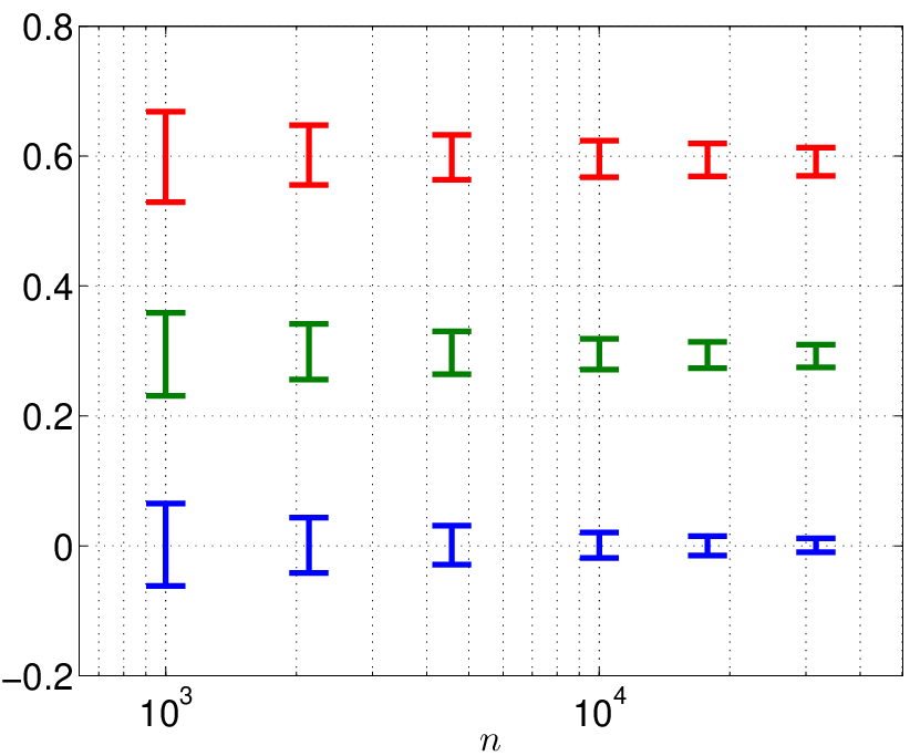
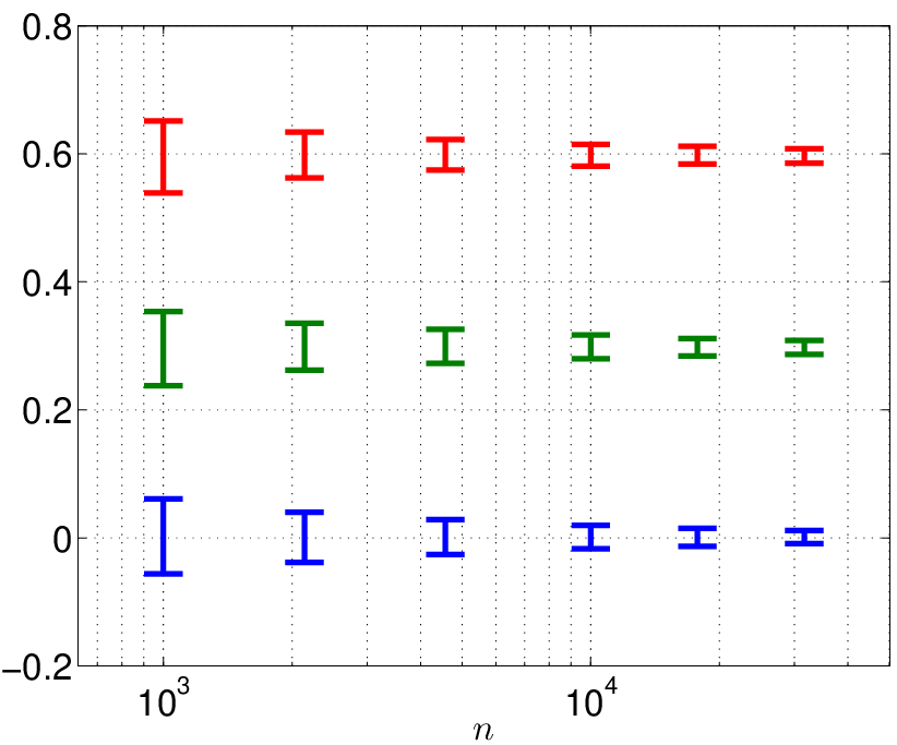
Fig. 1 presents the accuracy (mean and standard deviation) of the estimates of the class imbalance, achieved by the two different algorithms of Sections 1 and 4.2, vs. the number of unlabeled instances , for several values of the class imbalance, . As expected, the accuracy of both methods improves with the number of instances. Fig. 2 shows the mean squared error (MSE) vs. the number of samples , on a log-log scale. The linear line with slope shows that empirically , in accordance to Lemma 5. In addition, on simulated data, the restricted likelihood estimator is more accurate than the tensor-based estimator.

6.2 Real data
We applied our algorithms on various binary and multi-class problems using a total of 5 datasets: 4 datasets from the UCI repository (Bache and Lichman, 2013) and the MNIST data. Our ensemble consisted of classification methods implemented in the software package Weka (Hall et al., 2009). Due to page limits, we present here results only on the ’magic’ dataset. Further details on the different datasets, classifiers and additional results appear in the appendix.
The magic data contains instances with 11 attributes. The task is to distinguish each instance as either background or high energy gamma rays. Each of the classifiers was trained on its own randomly chosen set of 200 instances. The classifiers were then applied to the whole dataset, thus providing the prediction matrix. We compared the results of 4 different unsupervised ensemble methods: (i) Majority voting; (ii) SML of Parisi et al. (2014); (iii) i-SML as described in section 4; and (iv) Oracle ML: the MLE formula (8) with the values of and , estimated from the full dataset with its labels.
To assess the stability of the different methods, for each dataset we repeated the above simulation times, each realization with different randomly chosen training sets. Fig. 3(a) shows the mean and standard deviation of the balanced accuracy achieved by the four methods on the ’magic’ dataset. It shows that on average, i-SML improves upon the SML by approximately , and both are significantly better than majority voting. Fig. 3(b) displays the error rates vs. for all realizations. As all points are below the diagonal, the improvement over SML was consistent in all 30 simulation runs. As shown in the appendix, similar results, and in particular the improvement of i-SML over SML, were observed also in all 4 other datasets.
7 Summary and Discussion
In this paper we presented a simple spectral-based approach to estimate, in an unsupervised manner, the accuracies of multiple classifiers, mainly in the binary case. This, in turn, resulted in a novel unsupervised spectral ensemble learner, denoted i-SML. The empirical results on several real data sets attest to its competitive performance in practical situations where clearly the underlying idealized assumptions that all classifiers make independent errors do not hold exactly.
There are several interesting directions to extend this work. One possible direction is to relax the strict assumptions of independence of classifier errors across all instances, for example by introducing the concept of instance difficulty. A second interesting direction is the construction of novel semi-supervised ensemble learners, when one is given not only the predictions of classifiers on a large unlabeled set of instances, but also their predictions on a small set of labeled ones.


References
- Anandkumar et al. [2012a] A. Anandkumar, R. Ge, D. Hsu, S.M. Kakade, and M. Telgarsky. Tensor decompositions for learning latent variable models. arXiv preprint arXiv:1210.7559, 2012a.
- Anandkumar et al. [2012b] A. Anandkumar, D. Hsu, and S.M. Kakade. A method of moments for mixture models and hidden markov models. arxiv preprint arxiv:1203.0683, 2012b.
- Bache and Lichman [2013] K. Bache and M. Lichman. UCI machine learning repository, 2013.
- Dawid and Skene [1979] A. P Dawid and A. M Skene. Maximum likelihood estimation of observer error-rates using the em algorith. Journal of the Royal Statistical Society. Series C, 28:20–28, 1979.
- Dietterich [2000] T.G. Dietterich. Ensemble methods in machine learning. In Lecture Notes in Computer Science, volume 1857, pages 1–15. Springer, Berlin, 2000.
- Donmez et al. [2010] P. Donmez, G. Lebanon, and K. Balasubramanian. Unsupervised supervised learning I: Estimating classification and regression errors without labels. The Journal of Machine Learning Research, 11:1323–1351, 2010.
- Feldman et al. [2008] J. Feldman, R. O’Donnell, and R.A. Servedio. Learning mixtures of product distributions over discrete domains. SIAM Journal on Computing, 37(5):1536–1564, 2008.
- Freund and Mansour [1999] Y. Freund and Y. Mansour. Estimating a mixture of two product distributions. In COLT ’99 Proceedings of the twelfth annual conference on Computational learning theory, pages 53–62, 1999.
- Hall et al. [2009] M. Hall, E. Frank, G. Holmes, G. Pfahringer, P. Reutemann, and I.H Witten. The weka data mining software: An update. SIGKDD Explorations, 11(1), 2009.
- Jain and Oh [2013] P. Jain and S. Oh. Learning mixtures of discrete product distributions using spectral decompositions. arXiv preprint arXiv:1311.2972, 2013.
- Karger et al. [2011] D.R. Karger, S. Oh, and D. Shah. Budget-optimal crowdsourcing using low-rank matrix approximations. In IEEE Alerton Conference on Communication, Control and Computing, pages 284–291, 2011.
- Newey [1991] W. K. Newey. Uniform convergence in probability and stochastic equicontinuity. Econometrica, 59:1161–1167, 1991.
- Parisi et al. [2014] F. Parisi, F. Strino, B. Nadler, and Y. Kluger. Ranking and combining multiple predictors without labeled data. Proceedings of the National Academy of Sciences, 111:1253–1258, 2014.
- Platanios et al. [2014] E.A. Platanios, A. Blum, and T. Mitchell. Estimating accuracy from unlabeled data. In Uncertainty in Artificial Intelligence, 2014.
- Raykar et al. [2010] V.C. Raykar, Y. Shipeng, L.H. Zhao, G.H. Valdez, C. Florin, L. Bogoni, and Moy L. Learning from crowds. J. Machine Learning Research, 11:1297–1322, 2010.
- Rokach [2009] L. Rokach. Collective-agreement-based pruning of ensembles. Computational Statistics and Data Analysis, 53:1015–1026, 2009.
- Sheng et al. [2008] V.S. Sheng, F. Provost, and P.G. Ipeirotis. Get another label? improving data quality and data mining using multiple, noisy labelers. In Proceedings of the 14th ACM SIGKDD international conference on Knowledge discovery and data mining, pages 614–622, 2008.
- Sheshadri and Lease [2013] A. Sheshadri and M. Lease. Square: A benchmark for research on computing crowd concensus. In AAAI conference on human computation and crowdsourcing, 2013.
- Snow et al. [2008] R. Snow, B. O’Connor, D. Jurafsky, and A.Y. Ng. Cheap and fast but is it good? In Conference on Empirical Methods in Natural Language Processing, 2008.
- Welinder et al. [2010] P. Welinder, S. Branson, S. Belongie, and P. Perona. The multidimensional wisdom of crowds. In Advances in Neural Information Processing Systems 23 (NIPS 2010), 2010.
- Whitehill et al. [2009] J. Whitehill, P. Ruvolo, T. Wu, J Bergsma, and J.R. Movellan. Whose vote should count more: Optimal integration of labels from labelers of unknown expertise. In Advances in Neural Information Processing Systems 22 (NIPS 2009), 2009.
- Zhang et al. [2014] Y. Zhang, X. Chen, D. Zhou, and M.I. Jordan. Spectral methods meet em: A provably optimal algorithm for crowdsourcin. arXiv preprint arXiv:1406.3824, 2014.
Appendix A Estimation of and
Proof of Lemma 3.
We first recall the following formula, derived in Parisi et al. [2014], for the vector containing the mean values of the classifiers,
| (27) |
where denotes the vector containing half the difference between and ,
| (28) |
Next, recall from Lemma 1 (also proven in Parisi et al. [2014]) that the off-diagonal elements of the covariance matrix correspond to a rank-1 matrix where,
| (29) |
Inverting the relation between and in Eq. (29) gives
| (30) |
Plugging (30) into (27), we obtain the following expression for the vector , in terms of and ,
| (31) |
Combining (28), (30) and (31) we obtain and ,
∎
Appendix B Statistical Properties of and
Proof of Lemma 6.
Eq. (5) provides an explicit expression for and as a function of the estimates and . The empirical mean is clearly not only unbiased, but by the law of large numbers also a consistent estimate of , and its error indeed satisfies
The estimate , computed by one of the methods described in Parisi et al. [2014] may be biased, but as proven there is still consistent, and assuming at least three classifiers are different than random (in particular, implying that the eigenvalue of the rank one matrix is non-zero), its error also decreases as ,
Given the exact value of the class imbalance , since the dependency of and on and is linear, it follows that both are also consistent and that their estimation error is . ∎
Appendix C The joint covariance tensor
Proof of Lemma 4.
To simplify the proof, we first introduce the following linear transformation to the original classifiers,
Note, that the output space of the new classifiers is , with class probabilities equal to and respectively. Let us also denote by and the following probabilities,
Note that is not the specificity of classifier , but rather its complement, .
The mean of classifier , denoted , is given by
| (32) |
Next, let us calculate the (un-centered) covariance between two different classifiers ,
| (33) |
Last, the joint covariance between 3 different classifiers is given by
| (34) | |||||
The first step in calculating the joint covariance tensor of the original classifiers is to note that and . Hence,
where
Upon opening the brackets, the latter can be equivalently written as
| (35) |
Plugging (32),(33) and (34) into (35) we get,
| (36) |
Opening the brackets and collecting similar terms yields
| (37) |
Note that all polynomials in in the above expression are equal to . Hence,
| (38) |
Finally, replacing , and , yields
| (39) |
∎
Proof of Lemma 5.
To prove that is consistent with an asymptotic error , we first recall that according to Parisi et al. [2014], it follows that
By its definition, each entry of also incurs an error of . Hence, by the delta method, the estimate of Eq. (19), being a least squares minimizer, also satisfies
Since is found by the smooth relation of Eq. (17), again by the delta method, . Finally, the fact that the corresponding estimates and also have errors follows by standard application of the delta method to Eq. (5), where all quantities and have errors . ∎
Dependence of estimated parameters on number of classifiers and their accuracies.
Beyond the fact that and consequently are all consistent, it is of interest to study the dependence of these estimates on the number of classifiers and their accuracies. To this end, we first prove the following simple result.
Lemma 6.
Let be the estimate of in Eq. (19). Then asymptotically as , its estimation error is given by
| (40) |
where , and for any two tensors , .
Proof.
The minimizer of Eq. (19) is given by
According to Parisi et al. [2014], as , the estimate is consistent, namely , where . Writing where the latter is also and inserting these into the expression for above gives that
Next, recall that . Now, keeping only the leading order error terms yields Eq. (40). ∎
According to Eq. (40), the estimation error depends on the statistical properties of the deviations and and their correlations. While these are quite complicated, we may gain insight by looking at some particular instances. Assume for simplicity that all classifiers have comparable accuracies. Then, . Hence, the estimation error in should decrease with the number of classifiers. Moreover, for a balanced problem with and hence , to leading order, the errors in and consequently also in should not depend on the errors in estimating the eigenvector . Figure 4 shows this empirically. The -axis is the number of classifiers, the -axis is the mean absolute deviation (MAE), both on a log scale. We considered two values and , and for each value of we plotted two curves, one corresponding to the estimate computed from based on , and the second, an “oracle” one, where is estimated using the true . Indeed, for both curves nearly coincide, in accordance to Eq. (40). In this simulation, all classifiers had a balanced accuracy in the range , and . These results suggest that it is potentially profitable to estimate the eigenvector and the scalar jointly from both the covariance matrix and the tensor , and not separately as done in the present paper. This, as well as a more detailed study of the estimation errors are issues beyond the scope of the current work.

Appendix D The Restricted Likelihood Function
Proof of Theorem 1.
By definition, the function in Eq. (22) is the log-likelihood of the observed vector of predicted labels at an instance , assuming the class imbalance is and using the estimates and for the sensitivities and specificities of the classifiers.
Under the assumption that all classifiers make independent errors, the expression for is given by
| (41) |
We first prove Eq. (26), that upon using the exact log-likelihood function ), its mean is maximized at the true value . To this end, we write the expectation explicitly,
| (42) | |||||
Note the difference between the assumed class imbalance , which appears inside the logarithm, and its true value , over which we take the expectation.
To prove Eq. (26), let us first present the following auxiliary lemma, which can be easily proved using Lagrange multipliers.
Lemma 7.
Consider the following function of unknown variables ,
| (43) |
where are non-negative constants. Under the constraints that , and , the function has a global maxima at for all .
We use this lemma with and the following set of constants , over all possible -dimensional vectors , and the variables . The expectation of is now equal to
| (44) |
By Eq. (43), over all possible choices of , the expectation attains its maxima at for all . Since at , the corresponding probabilities , Eq. (26) follows.
Next, we wish to prove that in probability. To this end, we follow the approach outlined in Newey [1991], and prove the following uniform convergence in probability of to ,
This equation, coupled with the equicontinuity of implies the convergence in probability of the maximizer of (namely ) to that of , which by Eq. (26) is .
As proved in [Newey, 1991, Theorem 2.1], this uniform convergence in probability is satisfied if and only if there is pointwise convergence of to , and is stochastic equicontinuous. Fortunately, a sufficient condition for the latter property is that is continuously differentiable and its derivative bounded, see Newey [1991] Corollary 2.2 and discussion after it.
In our case, since , it suffices to prove that for any vector , the function is continuously differentiable with a bounded derivative. First note that by their definition, Eq. (5), the functions and are continuously differentiable with bounded derivative for all . Next, under the assumptions of the theorem, that and are bounded from 0 and from 1, and hence also their estimates can be restricted to , the term inside the logarithm in Eq. (22) is bounded away from zero. Hence, by its definition satisfies the required condition. ∎
Appendix E Ambiguity in the Multi-Class Case
Proof of Theorem 2.
For simplicity, let us assume that all class probabilities are equal, for . Let be the set of original classifiers with confusion matrices . We shall now construct another set of classifiers with different confusion matrices that nonetheless lead to the same values and for all subsets .
To this end, assume that all entries of the first confusion matrix are strictly positive and strictly smaller than one. Consider a second set of confusion matrices identical to the first, except for the following six changes in : For three fixed indices , let
where is sufficiently small so that all entries of are in .
Note that the new matrix is a valid confusion matrix, since for any column
Let be the classifier corresponding to the modified matrix . Next, note that the first order statistics of and of are unchanged. Indeed, by definition
If , then and thus
| (45) |
If , then by construction, in the -th row of there are precisely two modified entries, one increased by and the other reduced by , so overall the above equation still holds. Eq. (45) directly implies that for all subsets .
Next, let us show that the covariance matrices also remain unchanged. Recall that the entries of are determined by the values and . Hence, it suffices to show that for all subsets
| (46) |
To this end, recall that by definition
First consider the case . Here, all relevant entries in the sum for are unchanged. In contrast, the sum for includes all six modified entries. Both sums remain unchanged, and so Eq. (46) holds.
The proof for the other cases, where follows similar arguments.
To conclude, both and have the same values and covariance matrices . ∎
Appendix F Ensemble of Machine Learning Classifiers
Table 1 presents the 10 different classifiers used in our experiments. For each dataset, each classifier was trained with different (randomly chosen) instances.
| classifier | Weka library |
|---|---|
| IBk - K nearest | |
| neighbours, | lazy.IBk |
| KStar - Instance | |
| based classifier | lazy.KStar |
| J48 - Decision tree | trees.J48 |
| PART - Partial decision | |
| trees classifier | rules.PART |
| LMT - Logistic model | |
| trees | trees.LMT |
| Random forest - | |
| with trees | trees.RandomForest |
| Logistic Regression | functions.SimpleLogistic |
| Decision Stump - | |
| One level decision tree | trees.DecisionStump |
| Sequential Minimal | |
| Optimization | functions.SMO |
| NaiveBayes | bayes.NaiveBayes |
Appendix G Real Datasets
We tested our methods on a total of five datasets, 4 from the UCI repository and the MNIST digits data. A short description of each of the datasets is given in Table 2. A comparison of the performance of various ensemble learners on these datasets appears in Fig. 5.
| dataset | Task | instances | attributes |
|---|---|---|---|
| Magic | classifying gamma rays from background noise | 11 | |
| Spam | classifying spam from regular mail | ||
| Musk | classifying different types of molecules to be ’musk’ or ’non musk’ | ||
| Miniboo | distinguish electron neutrinos (signal) from muon neutrinos (background)’ | ||
| Mnist | To define a binary problem, we divided the MNIST data set into two classes as follows: vs. |


