KEK-TH-1755
De Sitter Vacua from
a D-term Generated Racetrack Uplift
Markus Rummel1 and Yoske Sumitomo2,
1Rudolph Peierls Centre for Theoretical Physics, University of Oxford,
1 Keble Road, Oxford, OX1 3NP, United Kingdom
2 High Energy Accelerator Research Organization, KEK,
1-1 Oho, Tsukuba, Ibaraki 305-0801 Japan
Email: markus.rummel at physics.ox.ac.uk, sumitomo at post.kek.jp
We propose an uplift mechanism using a structure of multi-Kähler moduli dependence in the F-term potential of type IIB string theory compactifications. This mechanism requires a D-term condition that fixes one modulus to be proportional to another modulus, resulting in a trivial D-term potential. De Sitter minima are realized along with an enhancement of the volume in the Large Volume Scenario and no additional suppression of the uplift term such as warping is required. We further show the possibility to realize the uplift mechanism in the presence of more Kähler moduli such that we expect the uplift mechanism to work in many other compactifications.
August 24, 2026
1 Introduction
Dark Energy is the dominant source causing the current accelerated expansion of the universe, as has been confirmed by observations [1, 2, 3, 4]. Although there exist some possibilities explaining Dark Energy, a tiny positive cosmological constant would be the prime candidate, in perfect agreement with recent observations [3, 4].
If one wants to understand the purely theoretically origin of this cosmological constant, we should promote Einstein gravity to be consistent with its quantum formulation. String theory is quite motivated for this purpose as it is expected to provide the quantum nature of gravity as well as particle physics. A cosmological constant could be realized in the context of flux compactifications [5, 6] of 10D string theories, where a vacuum expectation value of the moduli potential at minima contributes to the vacuum energy in a four-dimensional space-time universe. Since there exist many possible choices of quantized fluxes and also a number of types of compactifications, the resultant moduli potential including a variety of minima forms the string theory landscape (see reviews [7, 8, 9, 10, 11, 12]).
Although there exist many vacua in the string theory landscape, when we naively stabilize the moduli and obtain the minima, negative cosmological constants seem likely to come by. Hence an ’uplift’ mechanism from the negative vacuum energy keeping stability should be important to realize an accelerated expanding universe. Some possible ways of the uplift mechanism have been proposed in string compactifications.
- •
Explicit SUSY breaking achieved by brane anti-brane pairs contributes positively in the potential, and thus can be used for the uplift [13, 14, 15]. When the D3 brane anti-brane pairs are localized at the tip of a warped throat, the potential energy may be controllable due to a warping factor. As the uplift term contributes to the potential at , which appears larger than the F-term potential for stabilization which is in general , de Sitter () vacua with tiny positive cosmological constant may be achieved as a result of tuning of warping. A caveat of this proposal is that the SUSY breaking term needs to compensate the entire Anti-de Sitter () energy, so it is an open question if the SUSY breaking term, originally treated in a probe approximation, can be included as a backreaction in supergravity appropriately.
- •
As an alternative uplift mechanism, one may use the complex structure sector [16]. In the type IIB setup, the complex structure moduli as well as the dilaton are often stabilized at a supersymmetric point. Owing to the no-scale structure, the potential for the complex structure sector is positive definite . So when we stay at the SUSY loci, the potential is given convex downward in general and thus tractable. However, if one stabilizes the complex structure sector at non-supersymmetric points, then there appears a chance to have a positive contribution in the potential without tachyons, that may be applied for the uplift with a tuning. See also recent applications of this mechanism [17, 18, 19].
- •
When we include the leading order -correction coming of in the Kähler potential [20] which breaks the no-scale structure, this generates a positive contribution in the effective potential if the Euler number of the Calabi-Yau is given by a negative value [21]. This positive term can balance the non-perturbative terms in the superpotential such that stable vacua can be achieved in this Kähler Uplift model [22, 23, 24] (see also [25]). In the simplest version of the Kähler uplifting scenario, there is an upper bound on the overall volume of the Calabi-Yau such that one may worry about higher order -corrections. However, this bound can be significantly relaxed when embedded in a racetrack model [26].
- •
It has been proposed that the negative curvature of the internal manifold may be used for constructions as it contributes positive in the scalar potential [27]. Motivated by this setup, there were many attempts constructing vacua [28, 29, 30, 31, 32, 33, 34, 35, 36, 37, 38, 39, 40]. Using the necessary constraint for the extrema [41, 42] and for the stability [43], we see that the existence of minima requires not only negative curvature, but also the presence of orientifold planes.
- •
When the stabilization mechanism does not respect SUSY, D-terms can provide a positive contribution to the potential if the corresponding D7-brane is magnetically charged under an anomalous [44, 45, 46]. The potential of D-terms arises of order with , depending on the cycle that the D7-brane wraps. If we take into account the stabilization of matter fields having a non-trivial VEV, originating from fluxed D7-branes wrapping the large four-cycle, then the uplift contribution becomes [45]. So a relatively mild suppression, for instance by warping, is required for this volume dependence. See also recent applications to explicit scenarios in [47, 48] and also together with a string-loop correction in fibred Calabi-Yaus [49].
- •
Recently, it has been proposed that a dilaton-dependent non-perturbative term can also work for the uplift mechanism toward vacua [50]. The non-perturbative term depends on both the dilaton and a vanishing blow-up mode which is stabilized by a D-term. Since the D-term turns out to be trivial at the minima due to a vanishing cycle, the non-trivial dilaton as well as the vanishing cycle dependence generate the uplift term within the F-term potential. In this setup, the given uplift term is proportional to . Although the volume does not suppress the uplift term so much, we may expect an exponential fine-tuning by the dilaton dependence to balance with the moduli stabilizing F-term potential.
In this paper, we introduce an uplifting term of the form , where is the volume of a small 4-cycle, which naturally balances with the stabilizing F-term potential in the Large Volume Scenario (LVS). The following ingredients are necessary for this mechanism:
- •
one non-perturbative effect on a 4-cycle to realize the standard LVS moduli stabilization potential,
- •
another non-perturbative effect on a different cycle ,
- •
a D-term constraint that enforces the volumes of the two 4-cycles to be proportional via a vanishing D-term potential.
Hence, the minimal number of Kähler moduli for this uplifting scenario is . At the level of the F-term potential the effective scalar potential reduces to the standard LVS moduli stabilization potential plus the mentioned uplifting term yielding metastable vacua. The Kähler moduli are stabilized at large values avoiding dangerous string- and -corrections. Compared to [50], the dilaton can take rather arbitrary values determined by fluxes as there is no tuning required to keep the uplifting term suppressed. Note that for , a racetrack setup with two non-perturbative effects on one small cycle does not allow stable vacua in the LVS. Hence, we have to consider at least two small cycles and a relating D-term constraint to construct vacua.
We also have to consider a necessary condition for coexistence of the vanishing D-term constraint with the non-perturbative terms in superpotential. If the rigid divisors for the two non-perturbative effects intersect with the divisor on which the D-term constraint is generated via magnetic flux, we have to worry whether the VEV of matter fields that are generated by this magnetic flux are given accordingly such that the coefficients of non-perturbative terms remain non-zero. On the other hand, we may avoid additional zero mode contributions in a setup with minimal intersections. A general constraint is that the non-perturbative effects and D-term potential have to fulfill all known consistency condition, for instance requiring rigid divisors, avoiding Freed-Witten anomalies [51, 52] and saturating D3, D5, and D7 tadpole constraints. We expect these constraints to become less severe as the number of Kähler moduli increases beyond as in principle the degrees of freedom such as flux choices and rigid divisors increases.
This paper is organized as follows. We illustrate the uplift proposal generated through the multi-Kähler moduli dependence in the F-term potential and the required general geometric configuration in Section 2 and give some computational details in Appendix A. We further discuss the applicability of the uplift mechanism in more general Swiss-Cheese type Calabi-Yau manifolds in Section 3.
2 D-term generated racetrack uplift - general mechanism
We illustrate the uplift mechanism by a D-term generated racetrack in Calabi-Yaus with the following properties: there are two small 4-cycles and two linear combinations of these small cycles that are rigid such that the existence of two non-perturbative terms is guaranteed in the superpotential avoiding additional fermionic zero modes from cycle deformations or Wilson lines. We show that this setup in general allows to stabilize the moduli in a vacuum at large volume.
2.1 Geometric setup and superpotential
We consider an orientifolded Calabi-Yau with with the following general volume form of the divisors
| (2.1) |
in terms of 2-cycle volumes and intersection numbers
| (2.2) |
The 4-cycle volumes are given as
| (2.3) |
We assume that has a Swiss-Cheese structure with a big cycle named and at least two small cycles and , i.e., its volume form can be brought to the form
| (2.4) |
with parametrizing the dependence of the volume on the remaining moduli. Now let us assume there are two rigid divisors and of which a linear combination forms the small cycles and .
| (2.5) |
Even if there do not exist two divisors and that are rigid, one might still be able to effectively ‘rigidify’ one or more divisors by fixing all the deformation moduli of the corresponding D7-brane stacks via a gauge flux choice [53, 47, 54]. Under these assumptions, the superpotential in terms of the Kähler moduli is of the form
| (2.6) |
with non-zero , and being the Gukov-Vafa-Witten flux superpotential [55].
2.2 D7-brane and gauge flux configuration
The orientifold plane O7 induces a negative D7 charge of that has to be compensated by the positive charge of D7-branes. In general the O7 charge can be cancelled by introducing a Whitney brane with charge [56]. The non-perturbative effects of (2.6) can be either generated by ED3-instantons or gaugino condensation. For the latter, we choose a configuration with D7-branes on and D7-branes on . In this case, the exponential coefficients of the non-perturbative terms in (2.6) are and . The corresponding gauge group is either or (which becomes if gauge flux is introduced), depending on if the divisor lies on the orientifold plane or not. Furthermore we introduce a third stack of branes on a general linear combination of basis divisors that is not either or . This stack will introduce a D-term constraint that reduces the F-term effective scalar potential by one degree of freedom/ Kähler modulus. In the case of this corresponds to a two Kähler moduli LVS potential plus an uplift term that allows vacua as we will show in Section 2.3.11 1 In the case of being a linear combination of only and this divisor is only meaningful if and intersect as a linear combination of non-intersecting and rigid, i.e., local, four-cycles would not make sense. This is the reason we consider non-zero intersections between and in the first place as opposed to the more simple setup . Note that in general all required D7-brane stacks have to be consistent with possible factorizations of the Whitney brane that cancels the O7 charge [56, 57].
The D-term constraint is enforced via a Fayet-Illiopoulos (FI) term
| (2.7) |
where is the Kähler form on and is the anomalous -charge of the Kähler modulus induced by the magnetic flux on . We choose flux-quanta such that in (2.7) implies
| (2.8) |
with a constant depending on flux quanta and triple intersection numbers. In a concrete example it is important to check that a constant in (2.8) is realized which is consistent with stabilizing the moduli inside the Kähler cone of the manifold.
An important constraint arises from the requirement of two non-vanishing non-perturbative effects on generally intersecting cycles and . The cancellation of Freed-Witten anomalies requires the presence of fluxes on the D7-branes wrapping these divisors that can potentially forbid the contribution from gaugino condensation in the superpotential. This gauge invariant magnetic flux is determined by the gauge flux on the corresponding D7-brane and pull-back of the bulk -field on the wrapped four-cycle via
| (2.9) |
If and intersect each other, the -field can in general not be used to cancel both of theses fluxes to zero. However, it is still possible that both fluxes and can be chosen to be effectively trivial, such that no additional zero modes and FI-terms are introduced. These zero-modes would be generated via charged matter fields arising at the intersection of D7-brane stacks or from the bulk D7 spectrum. The constraint has to be checked on a case-by-case basis. We work out a sufficient condition on the intersections for and to be trivial for the case of and not intersecting any other divisors for in Appendix A. Furthermore, it has to be checked that does not generate any additional zero-modes at the intersections of with and .
Finally, the chosen D7-brane and gauge flux setup has to be consistent with D3, D5 and D7 tadpole cancellation. As for every explicit construction this has to be checked on a case-by-case basis for the particular manifold under consideration. We do not expect tadpole cancellation to be in general more restrictive than in e.g., the LVS. In particular, we do not require a large number of D7-branes [22] and/or racetrack effect [26] on a particular single divisor to achieve a large volume as in the Kähler Uplifting scenario.
2.3 Effective potential of the Kähler moduli
We start with a slightly simplified model where the F-term potential
| (2.10) |
is given by
| (2.11) |
where we have used equal intersection numbers and assumed stabilization of the dilaton and complex structure moduli via fluxes [5]. The values of these parameters are not essential for the uplift dynamics we illustrate in this paper. The superpotential in (2.11) corresponds to a particular choice of the general linear combination in (2.6). The model (2.11) is known to include the solutions of the LVS [58] that stabilizes the moduli in a non-supersymmetric way in the presence of the leading -correction [20] and one non-perturbative term. The -correction is given by where is the Euler number of the Calabi-Yau manifold.22 2 Recently, it has been argued that the leading correction in both and string coupling constants on structure manifold comes with the Euler characteristic of the six-dimensional manifold as well as Calabi-Yau compactifications [59].
The D-term potential is given through the magnetized D7-branes wrapping the Calabi-Yau divisor [60]:
| (2.12) |
where the gauge kinetic function
| (2.13) |
and are matter fields associated with the diagonal charges of a stack of D7-branes and the FI-term is defined in (2.7).
Now we redefine the coordinates:
| (2.14) |
When the D7-branes wrapping the divisor are magnetized and the matter fields are stabilized either at or satisfying , the D-term potential may become
| (2.15) |
using implied by the flux , see (2.8) where we use for simplicity. In the large volume limit, the F-term potential generically scales as in the minima given in the LVS model. Stabilizing the Kähler moduli at then requires a vanishing D-term potential, i.e., corresponding to .
Thanks to the topological coupling to the two-cycle supporting magnetic flux, the imaginary mode of the modulus is eaten by a massive gauge boson through the Stückelberg mechanism. Since the gauge boson has a mass of order of the string scale , the degree of freedom of charged under the anomalous as well as the gauge boson is integrated out at the high scale. Hence, we are left with the stabilization of the remaining moduli fields by the F-term potential.
2.4 F-term uplift
Next we will consider the stabilization by the F-term potential given in (2.11). We are interested in LVS like minima realizing an exponentially large volume. Then the leading potential of order is given by
| (2.16) |
where the imaginary directions are stabilized at , and is stabilized by non-perturbative effects that are omitted in (2.11), inducing a very small mass for and with negligible influence on the stabilization of the other moduli. Although the general minima of are given by with , the different solutions just change the sign of and thus we can simply have the potential of the above form.
As the D-term stabilizes , the resultant potential becomes
| (2.17) |
where we have defined . One may consider that this form of the potential looks similar to the racetrack type. Although cross terms of appear due to the dependence, the important point for the uplift mechanism demonstrated in this paper is that the cross terms between dependence of the term and dependence of the term appear at .33 3 Note that this would be more obvious if we start from a toy setup with , although one might not obtain the D-term constraint like . If the cross term appears at , it disturbs uplifting to .
We further redefine the fields and parameters such that there are no redundant parameters affecting the stabilization:
| (2.18) |
Then the effective potential at order becomes
| (2.19) |
We have neglected the term proportional to and the cross term between in the expression above. In fact, these terms are not important for the uplift mechanism of our interest, and we will justify this assumption a posteriori later. Since the uplift term comes together with , this term contributes of when . Hence, it contributes at the same order as the stabilizing F-term potential and no suppression factor provided by warping or dilaton dependence is required.
Before performing the uplift, we consider the LVS solution by setting . We use a set of parameters:
| (2.20) |
The extremal equations at can be simplified as
| (2.21) |
Solving the equations above, we obtain
| (2.22) |
We can easily check that this solution gives an vacuum. Note that when we have just two moduli fields in the LVS, the positivity of automatically guarantees the stability of the minima since the required condition is satisfied (see e.g. [61]).
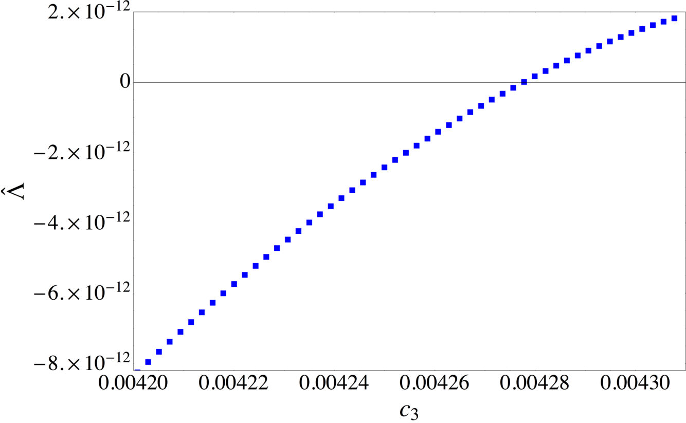
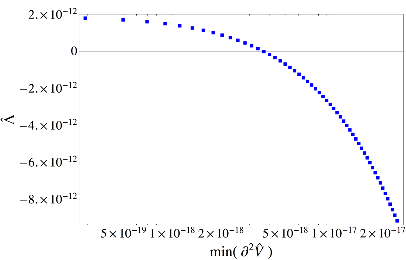
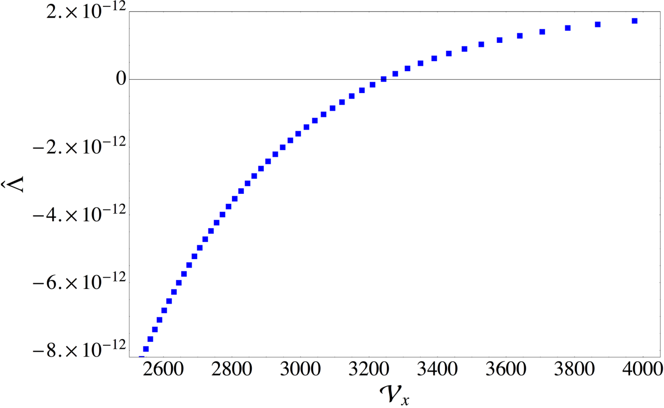
Now we consider non-zero for the uplift. As increases, the vacuum energy of the potential minimum increases and eventually crosses the Minkowski point. In Figure 1, we illustrate the behavior of the minimum point by changing the value of . Interestingly, the volume increases as the vacuum energy increases, suggesting that the effective description of the theory will be more justified toward vacua. On the other hand, the minimum value of the Hessian decreases. Destabilization occurs when the uplift term dominates the entire potential. As this happens at higher positive values of the cosmological constant, there certainly exist a range of parameters yielding stable vacua within this setup.
As a reference, we show numerical values of parameters close to crossing the Minkowski point. When we use
| (2.23) |
the minimum reaches Minkowski at
| (2.24) |
So we see that the volume increases quite drastically from the vacuum (2.22). Since remains small compared to the input value of , we see that our approximation neglecting the term proportional to is justified.
In fact, it is not difficult to see how these values change when the presence of terms and cross terms between in the potential (2.17) are taken into account. With the input parameters we used in (2.20), the Minkowski vacuum is obtained when
| (2.25) |
Since the obtained values are not significantly different from the case where terms and cross terms between are neglected, we conclude a posteriori that the uplift term is dominated by the term linear in .
Let us comment on the stabilization of the axionic partner of each modulus field. As stated, the imaginary mode of is eaten up by a massive gauge boson and hence integrated out at the high scale. The axionic partner of the big divisor is stabilized by non-perturbative effects yielding a tiny mass. The remaining modulus is stabilized by the F-term potential as the D-term potential does not depend on the latter. In the approximated potential up to , the Hessian of is
| (2.26) |
where we have included and cross terms, and used the solution (2.25) and . Thus all Kähler moduli are stabilized.
2.5 Analytical estimate
It is difficult to analytically derive a generic condition for the D-term generated racetrack uplift since the formulas are still complicated enough even after using several approximations. However, some of the expressions can be simplified under an additional reasonable approximation. In this subsection, we illustrate some analytical analyses for a better understanding.
Since we checked that the uplift mechanism works even at linear approximation of the uplift parameter , we only keep terms up to linear order in and neglect the higher order terms including cross terms. The extremal condition of the potential (2.19) is now simplified by
| (2.27) |
Although our interest is the uplift toward vacua, we have to cross the Minkowski point along the way. Thus, the condition that the minimum structure holds when uplifted to Minkowski vacua is a necessary condition for the uplift mechanism. The condition for Minkowski at the extrema reads
| (2.28) |
Next, we proceed to check the stability at the Minkowski point. Although we know the conditions to check the stability, the formula of the Hessian is yet too complicated to perform an analytical analysis. So we further focus on the region satisfying . The region with is motivated since the minimum points, before adding an uplift term, are guaranteed to have a positive Hessian since all eigenvalues are positive definite when satisfying in LVS type stabilizations (see e.g. [61]). Furthermore, higher instanton corrections can be safely neglected. As shown in Figure 1, the minima can be uplifted keeping the positivity of the Hessian until reaching the destabilization point with a relatively high positive vacuum energy. Hence, having is motivated to see the basic feature of the D-term generated racetrack uplift mechanism. Since there is no reason to take to be small/large, we consider .
When we use the approximation , a component of the Hessian and the determinant at the extrema become (2.27)
| (2.29) |
where in the last step of both equations, we have used the Minkowski condition (2.28). According to Sylvester’s criterion, the positivity of a matrix can be checked by the positivity of the determinant of all sub-matrices. Thus it is enough to check the positivity of the quantities in (2.29). Therefore we conclude that the stability at the Minkowski point requires . This condition is clearly satisfied in the previous numerical example following (2.23), which may justify the crude approximations we took in this subsection. Note that the Hessian of the imaginary mode is guaranteed to be positive under the above used approximations:
| (2.30) |
Finally, let us check the extremal and Minkowski conditions in the limit . Now all conditions are simplified to be
| (2.31) |
We see that the minimum point needs and in agreement with the minimum requirement of the two-moduli LVS at . The stability condition suggests . In fact, the extremal condition for is simply the leading order approximation of each first term in (2.27) as the contribution appears sub-dominant. This justifies that the linear approximation for is compatible with . Hence, we can regard the last term in the potential (2.19) as the uplift term.
3 On realization in models with more moduli
In this section, we show that the uplift mechanism works well in the presence of additional Kähler moduli in Swiss-Cheese type Calabi-Yau compactifications. We consider a simple toy model with , which captures the essential features of the D-term generated racetrack uplift mechanism defined by
| (3.1) |
Again we are interested in the case of a Swiss-Cheese volume for moduli stabilization of the LVS type. Note that we used the name to avoid confusion with .
Taking into account the D-term potential generated by the magnetized D7-branes wrapping the divisor , we assume again that the modulus is stabilized at . Setting for simplicity, the effective potential at from the F-terms is given by
| (3.2) |
where we have further defined and in addition to (2.18). Here we included the term proportional to as well as the cross term even though they are potentially subleading.
When we use a set of parameters:
| (3.3) |
then the LVS minimum at is located at
| (3.4) |
The stability of multi-Kähler moduli models of the LVS type is ensured if the constraint is satisfied [61]. Hence, the extremal point (3.4) is stable.
Now we add the uplift terms and . The minimum with the input parameters (3.3) reaches Minkowski at
| (3.5) |
Although the volume is drastically changed during the uplift toward vacua, we can check the stability of the minimum by plugging the values into the Hessian, similarly to the simple three moduli model. The cosmological constant can further increase in the positive region keeping the stability until the minima exceeds the potential barrier where decompactification happens.
4 Discussion
We have proposed an uplift mechanism using the structure of at least two small Kähler moduli and in Swiss-Cheese type compactifications. The uplift contribution arises as an F-term potential when using a D-term condition which fixes at a higher scale, where is determined by magnetized fluxes on D7-branes. The uplift term becomes of the form at large volumes, and hence it can naturally balance with the stabilizing potential in the Large Volume Scenario (LVS), without requiring suppressions in the coefficient, for instance, by warping or a dilaton dependent non-perturbative effect.
In addition, we have shown that the D-term generated racetrack uplift works in the presence of additional Kähler moduli. Together with the fact that constraints on the uplift parameters are rather relaxed, i.e., and , this makes us optimistic that there should be many manifolds admitting the proposed uplift mechanism.
Since the proposed uplift mechanism requires certain conditions for a D-term constraint and two non-vanishing non-perturbative effects, it should be interesting if we can construct an explicit realization of this model in a particular compactification. Such an explicit construction requires to match all known consistency conditions such as cancellation of Freed-Witten anomalies and cancellation of the D3, D5, and D7 tadpole [57, 47, 54, 48, 62]. We hope to report on an explicit example in another paper.
Furthermore, the phenomenological aspect of the proposed uplift mechanism should be interesting. Even though the moduli are essentially stabilized as in the LVS, the resultant behavior of the mass spectrum and/or soft SUSY breaking terms may be different depending on which uplift mechanism we employ to realize the vacuum.
Finally, in this paper, we concentrated on analyzing the structure of minima. However, the structure of the potential is also changed by the uplift term in regions that might be important for including inflationary dynamics. We relegate the analysis of possible inflation scenarios as well as phenomenological consequences compared to other uplift proposals to future work.
Acknowledgments
We would like to thank Joseph P. Conlon and Roberto Valandro for valuable discussions and important comments, and also the organizers of the workshop ”String Phenomenology 2014” held at ICTP Trieste, Italy, where some of the results of this paper were presented. YS is grateful to the Rudolph Peierls Centre for Theoretical Physics, University of Oxford where part of this work was done for their hospitality and support. MR is supported by the ERC grant ‘Supersymmetry Breaking in String Theory’. This work is partially supported by the Grant-in-Aid for Scientific Research (No. 23244057) from the Japan Society for the Promotion of Science.
Appendix A Conditions for avoiding additional zero-modes
In this appendix, we give a sufficient condition on the intersections for and to be trivial for the case of and not intersecting any other divisors for . This is a necessary condition for the non-perturbative effects on and to contribute to the superpotential, which is crucial for the uplift mechanism considered in this work.
In order to avoid Freed-Witten anomalies the gauge flux on the D7-branes has to satisfy
| (A.1) |
In particular, if is non-spin, i.e., is odd, is always non-zero. Using , the magnetic fluxes on and become
| (A.2) |
Since , and are all intersecting we have only one choice for the -field to cancel one . We choose the -field without loss of generality such that . In this case, we get
| (A.3) |
In order to avoid additional FI-terms and/or zero-modes via chiral matter at brane intersections or in the bulk spectrum of the D7-brane stacks on and , we have to demand the magnetic fluxes and to be effectively trivial which is the case for
| (A.4) |
for the Kähler form . This condition is trivially fulfilled for the zero flux . For , (A.4) becomes
| (A.5) |
using the intersection form (2.1). For general (A.5) is fulfilled if
| (A.6) |
where the last condition can be rewritten as . Clearly, (A.6) can not be fulfilled for general intersection numbers. The intersections that can accommodate the condition of trivial gauge flux and (A.6) are the following:
- •
or
- •
or
- •
, , with being an odd integer and integers or
- •
, , with being an odd integer and integers ,
i.e., for either of these conditions there exist flux quanta such that and are trivial. The second and fourth condition stem from choosing the -field such that .
References
- [1] Supernova Search Team Collaboration, A. G. Riess et al., “Observational evidence from supernovae for an accelerating universe and a cosmological constant,” Astron.J. 116 (1998) 1009–1038, arXiv:astro-ph/9805201 [astro-ph].
- [2] Supernova Search Team Collaboration, B. P. Schmidt et al., “The High Z supernova search: Measuring cosmic deceleration and global curvature of the universe using type Ia supernovae,” Astrophys.J. 507 (1998) 46–63, arXiv:astro-ph/9805200 [astro-ph].
- [3] C. Bennett et al., “Nine-Year Wilkinson Microwave Anisotropy Probe (WMAP) Observations: Final Maps and Results,” Astrophys.J.Suppl. 208 (2013) 20, arXiv:1212.5225 [astro-ph.CO].
- [4] Planck Collaboration Collaboration, P. Ade et al., “Planck 2013 results. XVI. Cosmological parameters,” arXiv:1303.5076 [astro-ph.CO].
- [5] S. B. Giddings, S. Kachru, and J. Polchinski, “Hierarchies from fluxes in string compactifications,” Phys.Rev. D66 (2002) 106006, arXiv:hep-th/0105097.
- [6] K. Dasgupta, G. Rajesh, and S. Sethi, “M theory, orientifolds and G - flux,” JHEP 9908 (1999) 023, arXiv:hep-th/9908088 [hep-th].
- [7] M. R. Douglas and S. Kachru, “Flux compactification,” Rev.Mod.Phys. 79 (2007) 733–796, arXiv:hep-th/0610102.
- [8] M. Grana, “Flux compactifications in string theory: A Comprehensive review,” Phys.Rept. 423 (2006) 91–158, arXiv:hep-th/0509003.
- [9] R. Blumenhagen, B. Kors, D. Lust, and S. Stieberger, “Four-dimensional String Compactifications with D-Branes, Orientifolds and Fluxes,” Phys.Rept. 445 (2007) 1–193, arXiv:hep-th/0610327 [hep-th].
- [10] E. Silverstein, “Les Houches lectures on inflationary observables and string theory,” arXiv:1311.2312 [hep-th].
- [11] F. Quevedo, “Local String Models and Moduli Stabilisation,” arXiv:1404.5151 [hep-th].
- [12] D. Baumann and L. McAllister, “Inflation and String Theory,” arXiv:1404.2601 [hep-th].
- [13] S. Kachru, J. Pearson, and H. L. Verlinde, “Brane / flux annihilation and the string dual of a nonsupersymmetric field theory,” JHEP 0206 (2002) 021, arXiv:hep-th/0112197.
- [14] S. Kachru, R. Kallosh, A. D. Linde, and S. P. Trivedi, “De Sitter vacua in string theory,” Phys.Rev. D68 (2003) 046005, arXiv:hep-th/0301240.
- [15] S. Kachru, R. Kallosh, A. D. Linde, J. M. Maldacena, L. P. McAllister, et al., “Towards inflation in string theory,” JCAP 0310 (2003) 013, hep-th/0308055.
- [16] A. Saltman and E. Silverstein, “The Scaling of the no scale potential and de Sitter model building,” JHEP 0411 (2004) 066, arXiv:hep-th/0402135 [hep-th].
- [17] U. Danielsson and G. Dibitetto, “An alternative to anti-branes and O-planes?,” JHEP 1405 (2014) 013, arXiv:1312.5331 [hep-th].
- [18] J. Blaback, J., D. Roest, and I. Zavala, “De Sitter Vacua from Non-perturbative Flux Compactifications,” arXiv:1312.5328 [hep-th].
- [19] R. Kallosh, A. Linde, B. Vercnocke, and T. Wrase, “Analytic Classes of Metastable de Sitter Vacua,” arXiv:1406.4866 [hep-th].
- [20] K. Becker, M. Becker, M. Haack, and J. Louis, “Supersymmetry breaking and alpha-prime corrections to flux induced potentials,” JHEP 0206 (2002) 060, hep-th/0204254.
- [21] V. Balasubramanian and P. Berglund, “Stringy corrections to Kahler potentials, SUSY breaking, and the cosmological constant problem,” JHEP 0411 (2004) 085, arXiv:hep-th/0408054 [hep-th].
- [22] A. Westphal, “de Sitter string vacua from Kahler uplifting,” JHEP 0703 (2007) 102, arXiv:hep-th/0611332.
- [23] M. Rummel and A. Westphal, “A sufficient condition for de Sitter vacua in type IIB string theory,” JHEP 1201 (2012) 020, arXiv:1107.2115 [hep-th].
- [24] S. de Alwis and K. Givens, “Physical Vacua in IIB Compactifications with a Single Kaehler Modulus,” JHEP 1110 (2011) 109, arXiv:1106.0759 [hep-th].
- [25] A. Westphal, “Eternal inflation with alpha-prime-corrections,” JCAP 0511 (2005) 003, arXiv:hep-th/0507079 [hep-th].
- [26] Y. Sumitomo, S. H. Tye, and S. S. Wong, “Statistical Distribution of the Vacuum Energy Density in Racetrack Kähler Uplift Models in String Theory,” JHEP 1307 (2013) 052, arXiv:1305.0753 [hep-th].
- [27] E. Silverstein, “Simple de Sitter Solutions,” Phys.Rev. D77 (2008) 106006, arXiv:0712.1196 [hep-th].
- [28] S. S. Haque, G. Shiu, B. Underwood, and T. Van Riet, “Minimal simple de Sitter solutions,” Phys.Rev. D79 (2009) 086005, arXiv:0810.5328 [hep-th].
- [29] R. Flauger, S. Paban, D. Robbins, and T. Wrase, “Searching for slow-roll moduli inflation in massive type IIA supergravity with metric fluxes,”Phys.Rev. D79 (Dec., 2009) 086011, 0812.3886.
- [30] U. H. Danielsson, S. S. Haque, G. Shiu, and T. Van Riet, “Towards Classical de Sitter Solutions in String Theory,” JHEP 0909 (2009) 114, arXiv:0907.2041 [hep-th].
- [31] C. Caviezel, T. Wrase, and M. Zagermann, “Moduli Stabilization and Cosmology of Type IIB on SU(2)-Structure Orientifolds,” JHEP 1004 (2010) 011, arXiv:0912.3287 [hep-th].
- [32] B. de Carlos, A. Guarino, and J. M. Moreno, “Flux moduli stabilisation, Supergravity algebras and no-go theorems,” JHEP 1001 (2010) 012, arXiv:0907.5580 [hep-th].
- [33] B. de Carlos, A. Guarino, and J. M. Moreno, “Complete classification of Minkowski vacua in generalised flux models,” JHEP 1002 (2010) 076, arXiv:0911.2876 [hep-th].
- [34] X. Dong, B. Horn, E. Silverstein, and G. Torroba, “Micromanaging de Sitter holography,” Class.Quant.Grav. 27 (2010) 245020, arXiv:1005.5403 [hep-th].
- [35] D. Andriot, E. Goi, R. Minasian, and M. Petrini, “Supersymmetry breaking branes on solvmanifolds and de Sitter vacua in string theory,” JHEP 1105 (2011) 028, arXiv:1003.3774 [hep-th].
- [36] U. H. Danielsson, P. Koerber, and T. Van Riet, “Universal de Sitter solutions at tree-level,” JHEP 1005 (2010) 090, arXiv:1003.3590 [hep-th].
- [37] U. H. Danielsson, S. S. Haque, P. Koerber, G. Shiu, T. Van Riet, et al., “De Sitter hunting in a classical landscape,” Fortsch.Phys. 59 (2011) 897–933, arXiv:1103.4858 [hep-th].
- [38] U. H. Danielsson, G. Shiu, T. Van Riet, and T. Wrase, “A note on obstinate tachyons in classical dS solutions,” JHEP 1303 (2013) 138, arXiv:1212.5178 [hep-th].
- [39] U. Danielsson and G. Dibitetto, “On the distribution of stable de Sitter vacua,” JHEP 1303 (2013) 018, arXiv:1212.4984 [hep-th].
- [40] J. Blaback, U. Danielsson, and G. Dibitetto, “Fully stable dS vacua from generalised fluxes,” JHEP 1308 (2013) 054, arXiv:1301.7073 [hep-th].
- [41] M. P. Hertzberg, S. Kachru, W. Taylor, and M. Tegmark, “Inflationary Constraints on Type IIA String Theory,” JHEP 0712 (2007) 095, arXiv:0711.2512 [hep-th].
- [42] T. Wrase and M. Zagermann, “On Classical de Sitter Vacua in String Theory,”Fortsch.Phys. 58 (Mar., 2010) 906–910, 1003.0029.
- [43] G. Shiu and Y. Sumitomo, “Stability Constraints on Classical de Sitter Vacua,” JHEP 1109 (2011) 052, arXiv:1107.2925 [hep-th].
- [44] C. Burgess, R. Kallosh, and F. Quevedo, “De Sitter string vacua from supersymmetric D terms,” JHEP 0310 (2003) 056, arXiv:hep-th/0309187.
- [45] D. Cremades, M.-P. Garcia del Moral, F. Quevedo, and K. Suruliz, “Moduli stabilisation and de Sitter string vacua from magnetised D7 branes,” JHEP 0705 (2007) 100, arXiv:hep-th/0701154 [hep-th].
- [46] S. Krippendorf and F. Quevedo, “Metastable SUSY Breaking, de Sitter Moduli Stabilisation and Kahler Moduli Inflation,” JHEP 0911 (2009) 039, arXiv:0901.0683 [hep-th].
- [47] M. Cicoli, S. Krippendorf, C. Mayrhofer, F. Quevedo, and R. Valandro, “D-Branes at del Pezzo Singularities: Global Embedding and Moduli Stabilisation,” JHEP 1209 (2012) 019, arXiv:1206.5237 [hep-th].
- [48] M. Cicoli, S. Krippendorf, C. Mayrhofer, F. Quevedo, and R. Valandro, “D3/D7 Branes at Singularities: Constraints from Global Embedding and Moduli Stabilisation,” JHEP 1307 (2013) 150, arXiv:1304.0022 [hep-th].
- [49] M. Cicoli, M. Goodsell, J. Jaeckel, and A. Ringwald, “Testing String Vacua in the Lab: From a Hidden CMB to Dark Forces in Flux Compactifications,” JHEP 1107 (2011) 114, arXiv:1103.3705 [hep-th].
- [50] M. Cicoli, A. Maharana, F. Quevedo, and C. Burgess, “De Sitter String Vacua from Dilaton-dependent Non-perturbative Effects,” JHEP 1206 (2012) 011, arXiv:1203.1750 [hep-th].
- [51] R. Minasian and G. W. Moore, “K theory and Ramond-Ramond charge,” JHEP 9711 (1997) 002, arXiv:hep-th/9710230 [hep-th].
- [52] D. S. Freed and E. Witten, “Anomalies in string theory with D-branes,” Asian J.Math 3 (1999) 819, arXiv:hep-th/9907189 [hep-th].
- [53] M. Bianchi, A. Collinucci, and L. Martucci, “Magnetized E3-brane instantons in F-theory,” JHEP 1112 (2011) 045, arXiv:1107.3732 [hep-th].
- [54] J. Louis, M. Rummel, R. Valandro, and A. Westphal, “Building an explicit de Sitter,” JHEP 1210 (2012) 163, arXiv:1208.3208 [hep-th].
- [55] S. Gukov, C. Vafa, and E. Witten, “CFT’s from Calabi-Yau four folds,” Nucl.Phys. B584 (2000) 69–108, arXiv:hep-th/9906070.
- [56] A. Collinucci, F. Denef, and M. Esole, “D-brane Deconstructions in IIB Orientifolds,” JHEP 0902 (2009) 005, arXiv:0805.1573 [hep-th].
- [57] M. Cicoli, C. Mayrhofer, and R. Valandro, “Moduli Stabilisation for Chiral Global Models,” JHEP 1202 (2012) 062, arXiv:1110.3333 [hep-th].
- [58] V. Balasubramanian, P. Berglund, J. P. Conlon, and F. Quevedo, “Systematics of moduli stabilisation in Calabi-Yau flux compactifications,” JHEP 0503 (2005) 007, hep-th/0502058.
- [59] M. Grana, J. Louis, U. Theis, and D. Waldram, “Quantum Corrections in String Compactifications on SU(3) Structure Geometries,” arXiv:1406.0958 [hep-th].
- [60] M. Haack, D. Krefl, D. Lust, A. Van Proeyen, and M. Zagermann, “Gaugino Condensates and D-terms from D7-branes,” JHEP 0701 (2007) 078, arXiv:hep-th/0609211 [hep-th].
- [61] M. Rummel and Y. Sumitomo, “Probability of vacuum stability in type IIB multi-Kähler moduli models,” JHEP 1312 (2013) 003, arXiv:1310.4202 [hep-th].
- [62] M. Cicoli, S. Krippendorf, C. Mayrhofer, F. Quevedo, and R. Valandro, “The Web of D-branes at Singularities in Compact Calabi-Yau Manifolds,” JHEP 1305 (2013) 114, arXiv:1304.2771 [hep-th].